141

A W i n e Method for Solid Model Display

Manjula Patel, Roger J. Hubbold f

AbShCt The modelling of solid objects is becoming increasingly important in the application of computer graphics to a wide variety of problems, such as CAD/CAM, simula- tion, and molecular modelling. A variety of methods for rendering solid objects exists, including 2-Buffer, Scanline and Ray Tracing. This paper is concerned with a scanline method for the production of still images of complex objects. The implementation of a scanline algorithm is discussed , in conjunction with a consideration of its performance in relation to the z- buffer method.

Many scanline methods cater only for a res- tricted class of primitives, such as polygons or spheres, whereas this implementation is a general purpose scan- line algorithm capable of being extended to handle a variety of primitives. The primitives currently available are polygons, spheres, spheres swept along straight-line trajectories, and cylinders. Polygonal models of cubes, cones and cylinders are also available.

The approach is capable of dealing with “posi- tive” and “negative” volumes, allowing objects with holes to be modelled and displayed. It has further been extended to cater for the inclusion of transparent objects into a scene, and consequently allows the modelling of coloured “glass” objects.

1. Introduction The modelling of three-dimensional (3-D) solid objects is important in a wide range of computer graphics applications, such as CAD/CAM, simulation, molecu- lar modelling and more recently in art and television advertising.

The motivation behind the work presented was to develop a convenient high-level interface for display- ing complex 3-D objects. The aim was to provide a tool for graphics progammers to use in a variety of applications, rather than a solid modelling system.

A number of representational forms have been developed for solid models:’ Primitive instancing

This paper was presented at the EUROGRAPHICS

’Department of Computer science, The University of ManChester =gtand

(UK) COnf~ren~e, Norwich, April 13-15 1987

North-Holland Computer Graphics Forum 6 (1987) 141-150

schemes, Spatial occupancy enumeration, Cell decom- position, Constructive Solid Geometry (CSG), Sweep representations and Boundary Representation (BR). The majority of solid modelling systems in use are either CSG or BR based.

CSG relies on the application of volumetric set operations to solid objects in order to represent more complex solid objects. The fundamental building blocks are solid objects or primitives. Two primitives can be combined to form a new solid object by apply- ing one of the Boolean set operators: Union, Intersec- tion or Difference. The systematic application of the set operations is usually described according to a binary tree structure. Each node defines the operation to be applied to its two children, while leaves indicate which solid primitives are to be used for processing.

Boundary modellers represent a solid by seg- menting its boundary into a finite number of bounded subsets, usually called faces or patches. Each face may in turn be represented by its bounding edges and vertices. Boundary representations are lengthy and consequently difficult to construct without computer assistance. Their main advantage is the ready availabil- ity of representations for faces, edges and the relations between them, this makes them ideal for incremental manipulation and modification of solid objects.

Since the impetus behind the project was the development of aesthetically pleasing images of 3-D objects rather than functional analysis, it was decided to adopt a primitive instancing scheme. Such approaches are easy for the naive user to grasp. Primi- tive instancing schemes are based on the notion of fam- ilies of objects, each member of a family being dis- tinguished by a small number of parameters. For example, a sphere might be represented by:

where x,, yc, z, are the coordinates of the centre and rad is the radius of the sphere.

Our implementation requires that any 3-D view- ing transformation be applied beforehand to the world coordinates that define the objects. A parallel projec- tion is assumed and calculations are performed in nor- malised projection coordinates or screen coordinates. A right-handed coordinate system is used.

142 M. Pate1 et al. f Scanline Method for Solid Model Disphy

2. Overview

To render primitives we employ a variation of the scan- line z-buffer technique. A scanline algorithm basically consists of two loops, one for the y-coordinate pro- gressing down the screen, and the other for the x- coordinate going across the screen for each y.

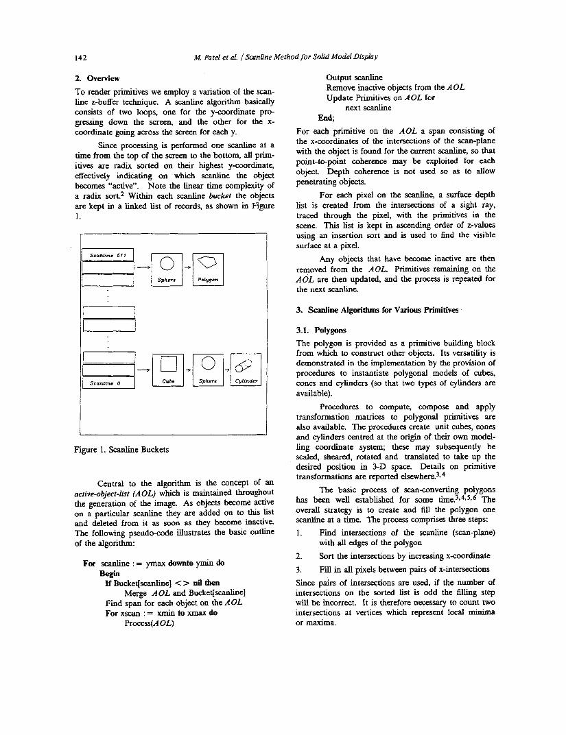
Since processing is performed one scanline at a time from the top of the screen to the bottom, all prim- itives are radix sorted on their highest y-coordinate, effectively indicating on which scanline the object becomes “active”. Note the linear time complexity of a radix sort? Within each Scanline bucket the objects are kept in a linked list of records, as shown in Figure 1 .

Figure 1. Scanline Buckets

Central to the algorithm is the concept of an active-object-list (AOL) which is maintained throughout the generation of the image. As objects become active on a particular scanline they are added on to this list and deleted from it as soon as they become inactive. The following pseudo-code illustrates the basic outline of the algorithm:

For Scanline : = ymax downto ymin do Besin

If Bucket[scanline] <> nil then Merge AOL and Bucket[scanline]

Find span for each object on the AOL For xscan : = xmin to xmax do

Process(A OL)

Output Scanline Remove inactive objects from the AOL Update Primitives on AOL for

next scanline End;

For each primitive on the AOL a span consisting of the xcoordinates of the intersections of the scan-plane with the object is found for the current scanline, so that point-to-pint coherence may be exploited for each object. Depth coherence is not used so as to allow penetrating objects.

For each pixel on the scanline, a surface depth list is created from the intersections of a sight ray, traced through the pixel, with the primitives in the scene. This list is kept in ascending order of z-values using an insertion sort and is used to find the visible surface. at a pixel.

Any objects that have become inactive are then removed from the AOL. Primitives remaining on the AOL are then updated, and the process is repeated for the next scanline.

3. Scanline Algorithms for Various Primitives

3.1. Polygons The polygon is provided as a primitive building block from which to construct other objects. Its versatility is demonstrated in the implementation by the provision of procedures to instantiate polygonal models of cubes, cones and cylinders (so that two types of cylinders are available).

Procedures to compute, compose and apply transformation matrices to polygonal primitives are also available. The procedures create unit cubes, cones and cylinders centred at the origin of their own model- ling coordinate system; these may subsequently be scaled, sheared, rotated and translated to take up the desired position in 3-D space. Details on primitive transformations are reported el~ewhere??~

The basic process of scanconverting polygons has been well established for some time.3,4.5,6 The overall strategy is to create and fill the polygon one scanline at a time. The process comprises three steps: 1 . Find intersections of the Scanline (scan-plane)

with all edges of the polygon 2. Sort the intersections by increasing x-coordinate 3. Fill in all pixels between pairs of x-intersections Since pairs of intersections are used, if the number of intersections on the sorted list is odd the filling step will be incorrect. It is therefore necessary to count two intersections at vertices which represent local minima or maxima.

M. Patel e t aL 1 Scanline Method for Solid Model Display 143

Finding the intersections between a scanline and a polygon can be time-consuming since each edge must be tested for intersection with each scanline. Scanline coherence (or edge coherence) is used to speed up the process since many of the edges intersected by scanline i will also be intersected by scanline i-1. As the y-scan progresses down from one scanline to the next, the new x-intersection of an edge (x,- ,) can be computed based on the old x-intersection (x,) .

For each scanline the edges it intersects are determined by an active-edge-list (AEL). In moving to the next scanline, new x-intersections are calculated from the old and any new edges intersected by the next scanline are added to the AEL using an insertion sort. Edges on the AEL not intersected by the next scanline are deleted. These changes may mean that the AEL is no longer in sorted order of x-intersections. A bubble sort is used in order to achieve this since it has a linear time complexity when the elements are nearly in sorted order?

Just as the x-y gradient of an edge is used in the linear interpolation of an edge in the x-y plane, the 2-y gradient is used to interpolate the depth values at the intersections. These depth values are then used to linearly interpolate the z-values in the x-z plane during the x-scan.

In order to make the addition of edges to the AEL efficient an edge table (ET) is created containing all edges sorted by their greater y-coordinate. The ET is built with a bucket (radix) sort using as many buck- ets as there are scanlines. Within each bucket, edges are kept in order of increasing x-coordinate of the higher endpoint, again by means of an insertion sort.

For the hidden surface removal and shading processes it is necessary to know whether a polygon is front-facing or back-facing. This information is acquired from the surface normal vector of the polygon, which depends on the direction of the vectors used to compute it. For consistency, it is assumed that vertices are ordered anti-clockwise when seen from the “outside”. This results in a vector which points towards the outside of a solid object.

3.2. Spheres Spheres are generated using an elementary Pythagorean method. In the x-y plane, given any scanline (y- coordinate) the x-value of the right-hand hemisphere is calculated. The span in the x-y plane is established using symmetry. To 6nd the z-values of the sphere for any point (x , y) within the span, Pythagoras is used in the x-z plane.

The unit surface normal i?, is required for shad- ing calculations. For a point ix, y, z) on a sphere with Centre (x,y,,z,) and radius r, N is given by:

N = r

l r

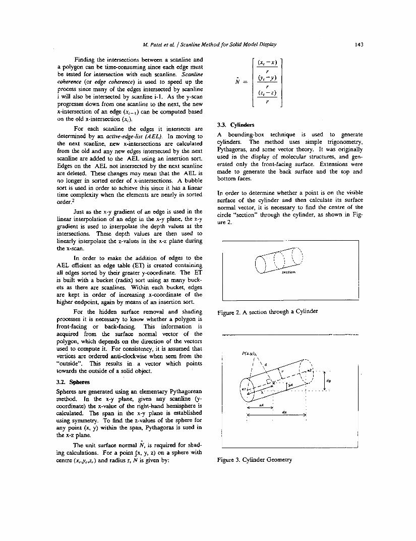
33. Cylinders A bounding-box technique is used to generate cylinders. The method uses simple trigonometry, Pythagoras, and some vector theory. It was originally used in the display of molecular structures, and gen- erated only the front-facing surface. Extensions were made to generate the back surface and the top and bottom faces.

In order to determine whether a point is on the visible surface of the cylinder and then calculate its surface normal vector, it is necessary to find the centre of the circle “section” through the cylinder, as shown in Fig- ure 2.

Figure 2. A section through a Cylinder

Figure 3. Cylinder Geometry

144 M. Pate1 et al. / Scanline Method for Solid Model Display

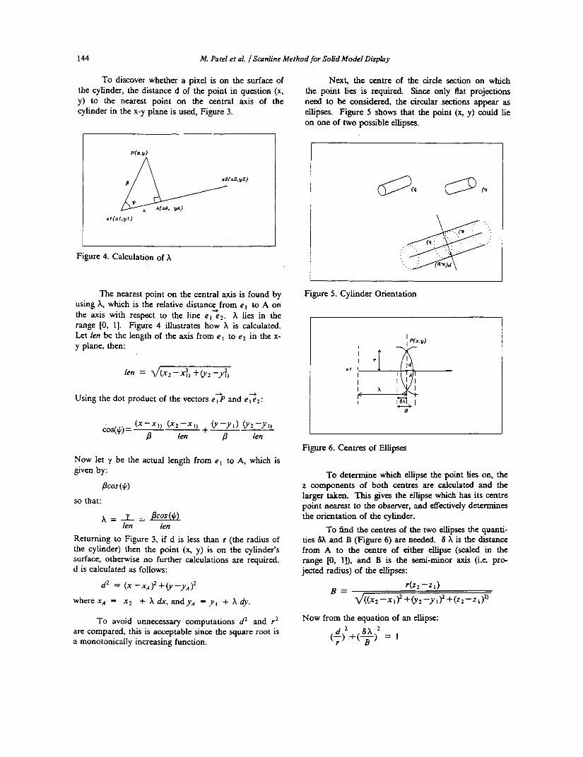
To discover whether a pixel is on the surface of the cylinder, the distance d of the point in question (x, y) to the nearest point on the central axis of the cylinder in the x-y plane is used, Figure 3.

Next, the centre of the circle section on which the point lies is required. Since only flat projections need to be considered, the circular sections appear as ellipses. Figure 5 shows that the point (x, y) could lie on one of two possible ellipses.

Figure 4. Calculation of X

The nearest point on the central axis is found by using A, which is the relative distanc2from e l to A on the a x i s with respect to the line e l ez. A lies in the range [0, 11. Figure 4 illustrates how X is calculated. Let len be the length of the axis from e l to e2 in the x- y plane, then:

4 Using the dot product of the vectors e? and e l e z :

Now let y be the actual length from e l to A, which is given by:

Bcos (4) so that:

x = r = L % , ! k l fen Ien

Returning to Figure 3, if d is less than r (the radius of the cylinder) then the point (x, y) is on the cylinder’s surface, otherwise no further calculations are required. d is calculated as follows:

d2 = ( X -xA)’ +@-Y,)~

wherex, = x 2 f Xdx, andy, = y I + X 4 .

To avoid unnecessary computations d 2 and r2 are compared, this is acceptable since the square root is a monotonically increasing function.

Figure 5. Cylinder Orientation

Figure 6. Centres of Ellipses

To determine which ellipse the point lies on, the z components of both centres are calculated and the larger taken. This gives the ellipse which has its centre point nearest to the observer, and effectivefy determines the orientation of the cylinder.

To find the Centres of the two ellipses the quanti- ties Sh and B (Figure 6) are needed. 6 X is the distance from A to the centre of either ellipse (scaled in the range [0, I]), and B is the semi-minor axis (i.e. pro- jected radius) of the ellipses:

Now from the equation of an ellipse:

M. Patel et aL 1 Scanline Method for Solid Model Displny 145

we have,

and scaling to the range [0, I]:

If 6 h is added to or subtracted from A, the centre points of the two ellipses are oktained in terms of the relative length along the line e l e l . The nearest centre point to the viewer is then taken as the required point.

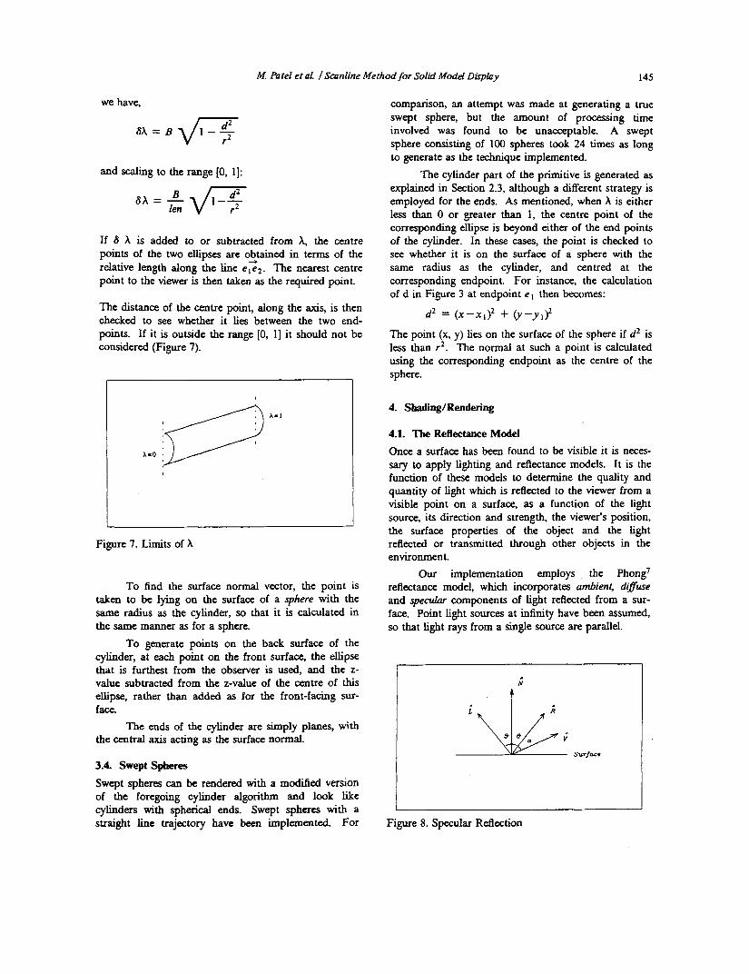
The distance of the eentre point, dong the axis, is then checked to see. whether it lies between the two end- points. If it is outside the range [0, 11 it should not be considered (Figure 7).

Figure 7. Limits of h

To find the surface normal vector, the point is taken to be lying on the surface of a sphere with the same radius as the cylinder, so that it is calculated in the same manner as for a sphere.

To generate points on the back surface of the cylinder, at each point on the front surface, the ellipse that is furthest from the observer is used, and the Z-

value subtracted from the z-value of the centre of this ellipse, rather than added as for the front-facing sur- face.

The ends of the cylinder are simply planes, with the central axis acting as the surface normal.

3.4. Swept Spheres Swept spheres can be rendered with a modified version of the foregoing cylinder algorithm and look like cylinders with spherical ends. Swept spheres with a straight line trajectory have been implemented. For

comparison, an attempt was made at generating a true swept sphere, but the amount of processing time involved was found to be unacceptable. A swept sphere consisting of 100 spheres took 24 times as long to generate as the technique implemented.

The cylinder part of the primitive is generated as explained in Section 2.3, although a different strategy is employed for the ends. As mentioned, when X is either less than 0 or greater than 1, the centre point of the corresponding ellipse is beyond either of the end points of the cylinder. In these cases, the point is checked to see whether it is on the surface of a sphere with the same radius as the cylinder, and centred at the corresponding endpoint. For instance, the calculation of d in Figure 3 at endpoint e l then becomes:

d2 = ( x - X I ) ’ + @-yI)’

The point (x. y) lies on the surface of the sphere if dZ is less than r 2 . The normal at such a point is calculated using the corresponding endpoint as the centre of the sphere.

4. Shading/Rendering

4.1. The Reflectance Model Once a surface has been found to be visible it is neces- sary to apply lighting and reflectance models. It is the function of these models to determine the quality and quantity of light which is reflected to the viewer from a visible point on a surface, as a function of the light source, its direction and strength, the viewer’s position, the surface properties of the object and the light reflected or transmitted through other objects in the environment.

Our implementation employs the Phong’ reflectance model, which incorporates ambient, diffwe and speculur components of light reflected from a sur- face. Point light sources at infinity have been assumed, so that light rays from a single source are parallel.

t ”

Figure L 8. Specular Reflection

146 M. Patel et al. / Scanline Method for Solid Model Display

The ambient, diffuse and specular components are linearly combined to give the intensity (0 at a pixel (see Figure 8):

I = &,[I, + ( I -I,,)COS(O)] + I, W(6)cos(a)N

where &, is the Diffuse-Reflection Coefficient [0, I ] I, is the intensity of the ambient light (1 - I,) is, th,e intensity of the point light source

cos(6) is L . N I, is the colour of the light source W(0) is the Sgecular Reflection Coefficient cos(a) is R . V N is the Shinyness Coefficient

In fact the implementation models two point light sources, so that

The intensity represented by equation 1 is evaluated for each of the Red, Green and Blue (RGB) components that make up the colour of the visible surface at a pixel.

A Genisco CGT3000 display was used to view the images. S-ince this has only 8 bits per pixel, either ran- dom or ordered dither (as specified by the user) is applied to the RGB components prior to computing the index to the Genisco’s video look-up table.

5. Transparency and Translucency Many hidden-surface removal algorithms can be adapted to cater for transparent surfaces. Most of them, including the scanline algorithm, assume that sight rays always travel in straight lines, and this presents difficulties in modelling light refraction.

In our implementation, when the frontmost sur- face is found to be transparent, it is necessary to deter- mine the next visible surface from the depth-list. The shading calculation is then a weighted sum of the indi- vidual shades calculated for the two surfaces:

I = t l , + ( I - t ) I 1

where: t is the Transparency Coefficient of the first surface [O. 11

t = 0 indicates that the surface is opaque t = 1 indicates that the surface is totally tran-

sparent (invisible)

I is the final intensity I I is the diffuse intensity for the first surface assum- ing it to be opaque. I2 is the diffuse intensity for the second surface assuming it to be opaque.

The process has been extended to deal with one or more consecutive transparent surfaces on a surface depth-list. The specular reflection of the frontmost sur- face is added in once the final diffuse intensity has been found.

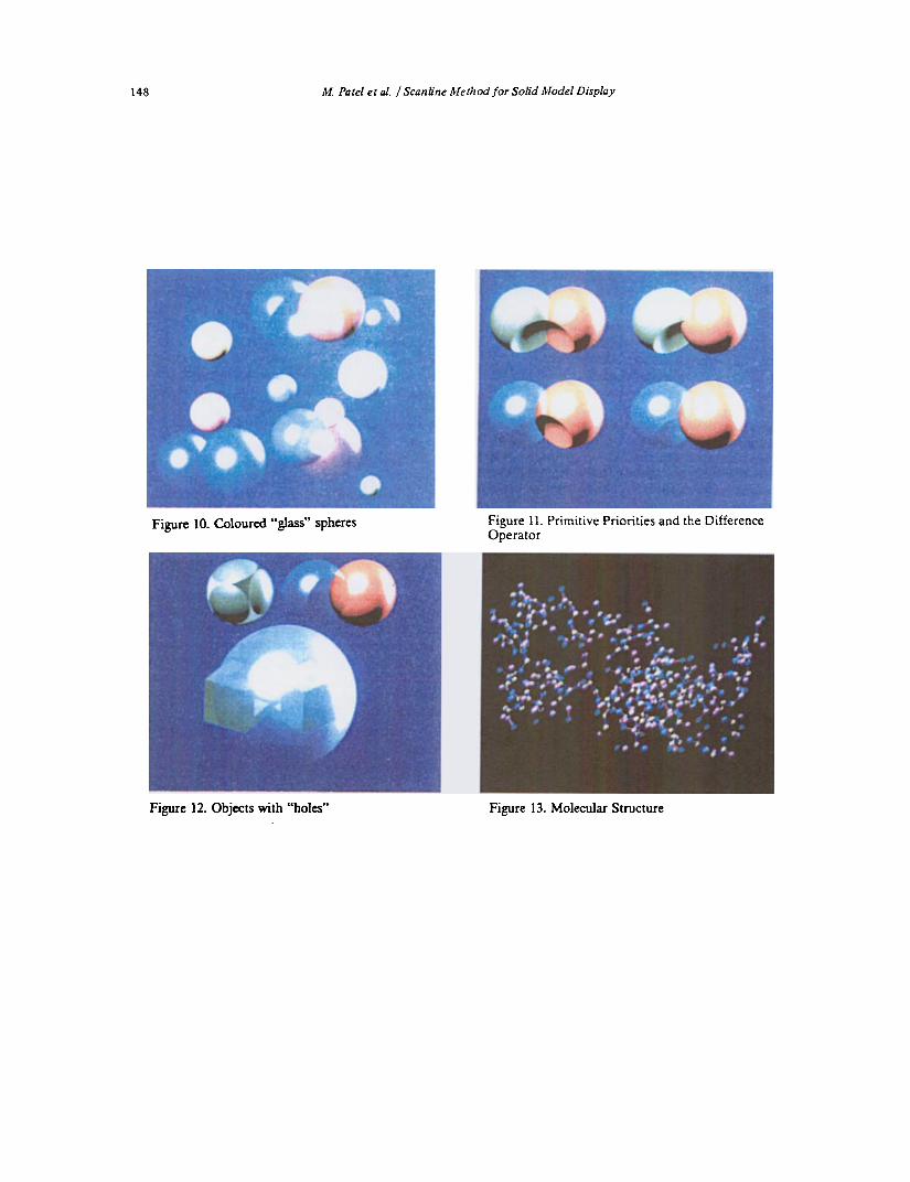
The implementation caters for transparent objects with holes, as well as allowing transparent objects that intersect or lie behind each other. Since the colour of any primitive is specified by the user, it is possible to have coloured “glass” objects within a scene. This is illustrated in Figure 10.

6. The Construction of Complex Objects More complex 3-D objects may be constructed from the primitives provided by employing the Boolean set operators, union and difference. Intersection as yet remains unimplemented.

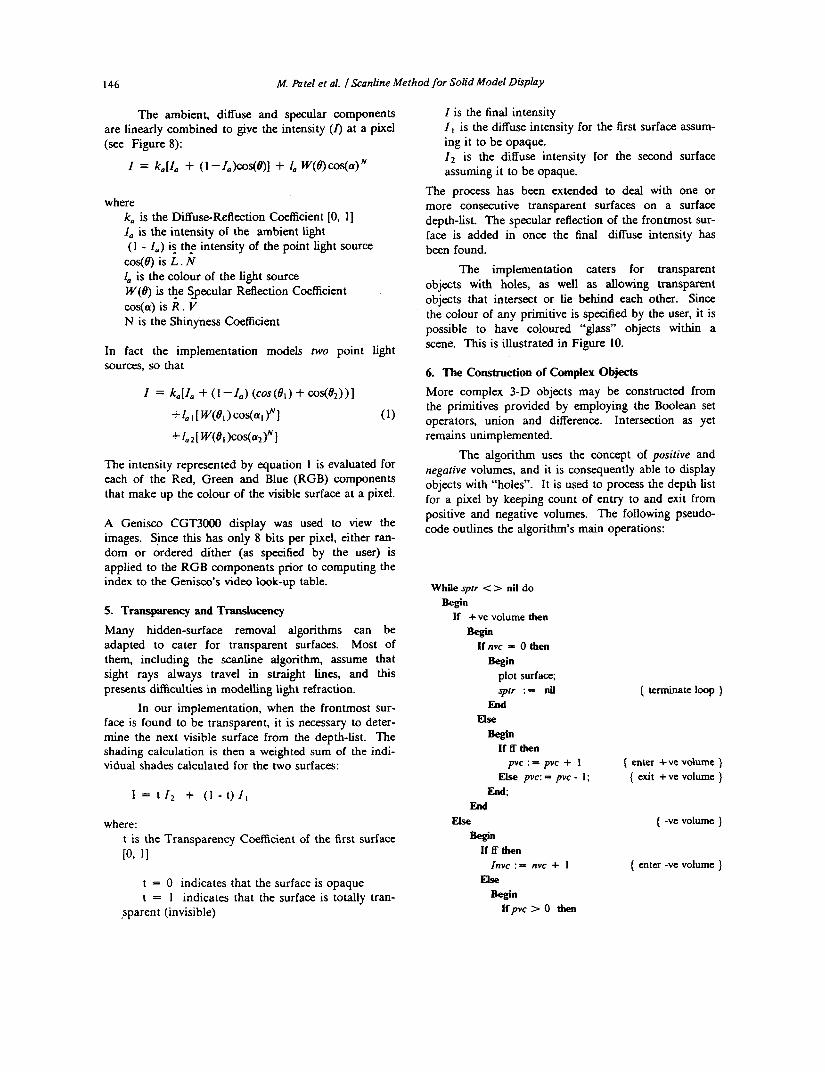
The algorithm uses the concept of positive and negafive volumes, and it is consequently able to display objects with “holes”. It is used to process the depth list for a pixel by keeping count of entry to and exit from positive and negative volumes. The following pseudo- code outlines the algorithm’s main operations:

( termhate loop )

While sptr <> nil do Begin

If +ve volume then

If nvc - 0 then Begin

Begin plot surface; sptr : = nil

End Else Begin

If ff then pvc :- pvc + 1

Else pvc:= pvc - 1; ( enter +ve volume ) ( exit + ve volume )

End; End

Else ( -ve volume ) Begin

If ff then

Else Znvc : - nvc + 1 ( enter -ve volume )

Begin lfpvc > 0 then

147 M. Pate1 et d. 1 Scanline Method for Solid Model Display

Begin plot surface; sptr : = nil; ( terminate loop ]

End

nvc := nvc- 1; ( exit -ve volume ] Else

End; End;

If spfr <> nil then sptr := spthext;

End;

where: sptr is a surface pointer which points to

nvc is the negative volume count pvc is the positive volume count fl represents front-facing

the list of surfaces at a pixel

The surface depth-list at a pixel is passed to the above routine, which after processing, returns a list with the visible surface at the head of it. A list is returned rather than the pixel intensity since the frontmost sur- face may be transparent, in which case the depth-list will require further processing to determine the next visible surface. The ultimate visible surface at a pixel is determined according to the positions of the primitives in 3-D space, and whether they are solids or voids. Extensions were made to allow the incorporation of transparent objects.

C C

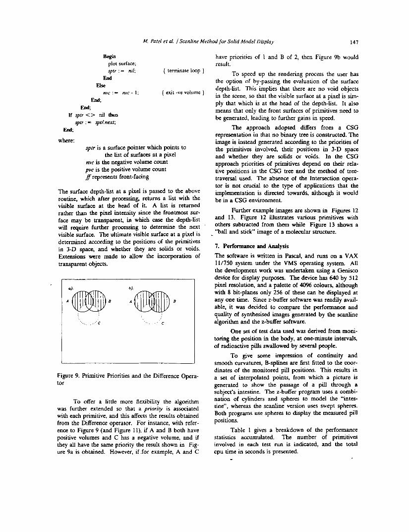
Figure 9. Primitive Priorities and the Difference Opera- tor

To offer a little more flexibility the algorithm was further extended so that a priority is associated with each primitive, and this affects the results obtained from the Difference operator. For instance, with refer- ence to Figure 9 (and Figure 11). if A and B both have positive volumes and C has a negative volume, and if they all have the same priority the result shown in Fig- ure 9a is obtained. However, if.for example, A and C

have priorities of 1 and B of 2, then Figure 9b would result.

To speed up the rendering process the user has the option of by-passing the evaluation of the surface depth-list. This implies that there are no void objects in the scene, so that the visible surface at a pixel is sim- ply that which is at the head of the depth-list. It also means that only the front surfaces of primitives need to be generated, leading to further gains in speed.

The approach adopted differs from a CSG representation in that no binary tree is constructed. The image is instead generated according to the priorities of the primitives involved, their positions in 3-D space and whether they are solids or voids. In the CSG approach priorities of primitives depend on their rela- tive positions in the CSG tree and the method of tree- traversal used. The absence of the Intersection opera- tor is not crucial to the type of applications that the implementation is directed towards, although it would be in a CSG environment.

Further example images are shown in Figures 12 and 13. Figure 12 illustrates various primitives with others subtracted from them while Figure 13 shows a “ball and stick“ image of a molecular structure.

7. Performance and Analysis

The software is written in Pascal, and runs on a VAX 11/750 system under the V M S operating system. AU the development work was undertaken using a Genisco device for display purposes. The device has 640 by 5 12 pixel resolution, and a palette of 4096 colours, although with 8 bit-planes only 256 of these can be displayed at any one time. Since z-buffer software was readily avail- able, it was decided to compare the performance and quality of synthesised images generated by the scanline algorithm and the z-buffer software.

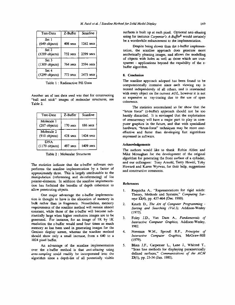
One set of test data used was derived from moni- toring the position in the body, at one-minute intervals, of radioactive pills swallowed by several people.

To give some impression of continuity and smooth curvatures, B-splines are first fitted to the coor- dinates of the monitored pill positions. This results in a set of interpolated points, from which a picture is generated to show the passage of a pill through a subject’s intestine. The z-buffer program uses a combi- nation of cylinders and spheres to model the “intes- tine”, whereas the scanline version uses swept spheres. Both programs use spheres to display the measured p d positions.

Table 1 gives a breakdown of the performance statistics accumulated. The number of primitives involved in each test run is indicated, and the total cpu time in seconds is presented. -

148 M Pate1 e t al. 1 Scanline Method for Solid Model Display

Figure 10. Coloured “glass” spheres Figure 11. Primitive Priorities and the Difference Operator

Figure 12. Objects with “holes” Figure 13. Molecular Structure

M. Patel et al. Scanline Method for Solid Model Display 149

Table 1 : Radioactive Pill Data

Another set of test data used was that for constructing “ball and stick” images of molecular structures, see Table 2.

Molecule 1

Molecule 2

Table 2 : Molecular Structures

The statistics indicate that the z-buffer software out- performs the scanline implementation by a factor of approximately three. This is largely attributable to the manipulation (referencing and de-referencing) of list pointer-elements. In addition the scanline implementa- tion has forfeited the benefits of depth coherence to allow penetrating objects.

One major advantage the z-buffer implementa- tion is thought to have is the allocation of memory in bulk rather than in fragments. Nonetheless, memory requirements of the scanline method will remain almost constant, while those of the z-buffer will become sub- stantially large when higher resolution images are to be generated. For instance, for an image of 1K by 1K resolution the z-buffer would need four times as much memory as has been used in generating images for the Genisco display screen, whereas the SCanline method should show only a small increase, from a 640 to a 1024 pixel buffer.

An advantage of the scanline implementation over the z-buffer method is that anti-aliasing using area-sampling could readily be incorporated into the algorithm since a depth-list of all potentially visible

surfaces is built up at each pixel. Optional anti-aliasing using for instance Carpenter’s A-Buflefi would certainly be a worthwhile enhancement to the implementation.

Despite being slower than the z-buffer implemen- tation, the scanline approach does generate more aesthetically pleasing images, and allows the modelling of objects with holes as well as those which are tran- sparent - applications beyond the capability of the z- buffer algorithm.

8. Condusion

The Scanline approach adopted has been found to be computationally intensive since each viewing ray is treated independently of all others, and is intersected with every object on the current AOL, however it is not as expensive as ray-tracing due to the use of span coherence.

The statistics accumulated so far show that the “brute force” (2-buffer) approach should not be too hastily discarded. It is envisaged that the exploitation of concurrency will have a major part to play in com- puter graphics in the future, and that with specialised hardware, “brute-force’’ techniques may be more cost- effective and faster than developing fast algorithms expressed in software.

Acknowledgements The authors would like to thank Robin Alden and Mike Monaghan for the development of the original algorithm for generating the front surface of a cylinder, and our colleagues: Tony Arnold, Terry Hewitt, Toby Howard and Karen Wynvas, for their help, suggestions and constructive comments.

References

1.

2.

3.

4.

5 .

Requicha A., “Representations for rigid solids: Theory, Methods and Systems,” Computing Sw- veys 12(4), pp. 437-464 (Dec. 1980).

Knuth D., The Art of Computer Programming - Sorting and Searching (voi.3). Addison-Wesley (1973). Foley J.D., Van Dam A., Fundamentals of Interactive Computer Graphics, Addison-Wesley, 1982. Newman W.M., Sproull R.F., Principles of Interactive Computer Graphics, McGraw-Hill ( 1979). Blinn J.F., Carpenter L., Lane J., Whitted T., “Scan line methods for displaying parametrically defined surfaces,” Communications of the ACM 23(1), pp. 23-34 (Jan. 1980).

150 M. Patel et al. 1 Scanline Method for Solid Model Display

6. Whitted T., “An improved Illumination model for I984 Proceedings Computer Graphics 18(3),

Patel M., ScanIine Methocis for Solid Modelling, University of Manchester (1986). MSc. Thesis

Gouraud H., “Continuous shading of curved s ~ - faces,’’ IEEE Transactions on Computers C-20(6), pp. 263-628 (June 1971).

shaded display,” Communications of the ACM pp. 103-108. 23(6), pp. 343-349 (June 1980). Phong Bui-Tuong, “Illumination for computer- generated pictures,” Communications .f the ACM 18(6), pp. 3 1 1-3 17 (June 1976). Carpenter L., “The A-Buffer, an Anti-Aliasing hidden surface removal method,” ACM Siggruph

9.

10. 7.

8.