A Scalable Cellular Implementation of

Parallel Genetic Programming

Gianluigi Folino, Clara Pizzuti and Giandomenico Spezzano

ICAR-CNR

c/o DEIS, Universita della Calabria

Via Pietro Bucci 41C

87036 Rende (CS), Italy

email:{folino, pizzuti, spezzano}@isi.cs.cnr.it

July 7, 2009

Abstract

A new parallel implementation of genetic programming based on the cellular model is

presented and compared with both canonical genetic programming and the island model

approach. The method adopts a load balancing policy that avoids the unequal utilization of

the processors. Experimental results on benchmark problems of different complexity show the

superiority of the cellular approach with respect to the canonical sequential implementation

and the island model. A theoretical performance analysis reveals the high scalability of the

implementation realized and allows to predict the size of the population when the number

of processors and their efficiency are fixed.

Keywords: genetic programming, parallel processing, cellular GP model, load

1

balance, scalability.

1 Introduction

Genetic programming (GP ) [22, 23, 25] is an extension of genetic algorithms (GAs)(and more

broadly evolutionary algorithms) that induces computer programs, usually represented as trees.

A genetic program system evolves iteratively a population of trees, having variable size, by ap-

plying variation operators. Each individual encodes a candidate solution and is associated with

a fitness value that measures the goodness-of-fit of that solution. The capability of genetic pro-

gramming in solving challenging problems, coming from different application domains, has been

largely recognized. Many problems have been solved by means of GP . For difficult problems,

however, in order to find a good solution, GP may require large number of generations by using

a population of sufficient size. The choice of population size is determined by the complexity of

the problem. It is well known that evaluating fitness is the dominant time consuming task for

GP and evolutionary algorithms in general. The necessity of high computational resources, both

in terms of memory, to store big populations of trees, and in terms of time, to evaluate the fitness

of the individuals in the population, may degrade GP performance drastically when applied to

large difficult problems. There has been recent increasing interest in realizing high-performance

GP implementations to extend the number of problems that GP can cope with. To this end, dif-

ferent approaches to parallelize GP have been studied and proposed [6, 8, 10, 19, 20, 28, 30, 34].

An extensive survey on the subject can be found in [37]. Differently from parallel genetic algo-

rithms [2, 3], for which it has been found experimentally that their behavior is generally better

than their sequential counterpart, parallel GP implementations produce controversial outcomes

[32].

2

This paper presents a parallel GP implementation, called CAGE (CellulAr GEnetic pro-

gramming), on distributed-memory parallel computers based on the fine-grained cellular model.

Preliminary results of the implementation were presented in [12]. CAGE is endowed with a load

balancing mechanism that distributes the computational load among the processors equally. Ex-

periments on classical test problems show that the cellular model outperforms both the sequential

canonical implementation of GP and the parallel island model. A theoretical study of the per-

formances, based on the isoefficiency function, reveals the high scalability of the system and

allows predicting the size of the problem when the number of processors and a given efficiency

(the percentage of utilization of processors) are fixed. The main novelties are the following:

• CAGE is the first parallel implementation of GP through the cellular model;

• the cellular implementation yields the same results of parallel genetic algorithms [2, 37],

that is, the multi-population case generally needs fewer evaluations to get the same solution

quality as a single-population case with the same total number of individuals;

• the very good performances of CAGE run counter to the widespread belief that parallel

GP is not suitable for cellular models [37] because of the varying size and complexity of the

individuals that makes cellular implementations of GP difficult both in terms of memory

and efficiency.

The paper is organized as follows. Section 2 proposes the main parallel models. Section 3

provides an overview of the parallel implementations. Section 4 presents the cellular parallel

implementation of GP. Section 5 evaluates the scalability of CAGE by using the isoefficiency

function. Section 6 presents the results of the method on some well-known benchmark problems

and validates the theoretical performance analysis on two of those problems. Furthermore, the

3

benefits of the proposed load balancing technique are showed. Finally, Section 7 presents a

comparison between our cellular model method and some island model implementations of GP .

2 Parallel Genetic Programming

GP belongs to the class of evolutionary algorithms and, as such, shares the same parallelization

features of evolutionary techniques. A classification of the approaches for parallelizing GP

includes three main models [2, 37]: the global model, the coarse-grained (island) model [26], and

the fine-grained (grid) model [31].

In the global model, the fitness of each individual is evaluated in parallel on different proces-

sors. A master process manages the population by assigning a subset of individuals to a number

of slave processes. During the evaluation there is no communication among the processors. At

the end of the evaluation the master collects the results and applies the variation operators to

generate the new population. This model is easy to implement but a main problem, as observed

in [37], can be a load imbalance, which decreases the utilization of the processors due to presence

in the population of trees of different sizes.

The island model divides a population P of M individuals into N subpopulations D1,

. . . ,DN , called demes, of M/N individuals. A standard GP algorithm works on each deme

and is responsible for initializing, evaluating, and evolving its own subpopulation. Subpopu-

lations are interconnected according to different communication topologies and can exchange

information periodically by migrating individuals from one subpopulation to another. The

number of individuals to migrate (migration rate), the number of generations after which mi-

gration should occur (frequency), the migration topology, and the number of subpopulations are

all parameters of the method that must be set.

4

In the grid model (also called cellular [41]) each individual is associated with a spatial loca-

tion on a low-dimensional grid. The population is considered as a system of active individuals

that interact only with their direct neighbors. Different neighborhoods can be defined for the

cells. The most common neighborhoods in the two-dimensional case are the 4-neighbor (von

Neumann neighborhood) consisting of the North, South, East, West neighbors and 8-neighbor

(Moore neighborhood) consisting of the same neighbors augmented with the diagonal neighbors.

In the ideal case, one processor is assigned to each grid point, thus fitness evaluation is per-

formed simultaneously for all the individuals. In practical implementations, however, this is not

true because the number of processors generally does not coincide with the number of points

on the grid. Selection, reproduction, and mating take place locally within the neighborhood.

Information diffuses slowly across the grid, giving rise to the formation of semi-isolated niches of

individuals having similar characteristics. The choice of the individual to mate with the central

individual and the replacement of the latter with one of the offspring can be accomplished in

several ways.

Ref. [37] noted that parallel genetic algorithms are faster than their sequential counterpart

and benefit from the multi population approach in two different aspects. First, the problem

of premature convergence is reduced thanks to the spatial isolation of the subpopulations that

co-evolve independently but promote local search. Second, the same solution quality can be

obtained in fewer generations, by using many populations instead of a single population with

the same total number of individuals.

The same results, however, have not been obtained for the coarse-grained parallel implemen-

tations of GP . In fact, although Koza [1, 24] reported a super-linear speedup for the 5-parity

problem, for other problems, Punch [32] found poorer results of convergence with respect to the

5

canonical GP . A systematic study on the performances of parallel genetic programming has

not been conducted. Punch [32] was the first to analyze the behavior of distributed GP with

respect to sequential GP. In the next section, we review the main parallel implementations of

GP. Next, after the description of CAGE, we compare the few experimental results available in

the literature with our approach.

3 Related Work

The most famous coarse-grained parallel implementation of GP is due to Koza and Andre [24, 1].

They used a PC 486 computer as host and a network of 64 transputers as processing nodes.

For the Even-5 parity problem, they obtained a super-linear speedup using a population of

32000 individuals, 500 on each node and a migration rate of 8% in the four directions of each

subpopulation at each generation.

Juille and Pollack [19, 20] described a parallel implementation of GP on a SIMD system.

Each SIMD processor simulated a computer program by using a simple instruction set defined

specifically for GP . S-expressions were evaluated efficiently, precompiling them in a postfix

program. The authors, for few classical problems, reported the execution time for one run and

the average execution time for one generation. For cos2x, using a population of 4096 individuals,

one per processor, they found a solution after an average of 17.5 generations with an average

execution time of 30.48 seconds.

Stoffel and Spector [35] described a high-performance GP system (HiGP) based on a virtual

stack machine (similar to [20]) that executed GP programs represented as fixed-length strings.

HiGP manipulated and generated linear programs instead of tree-structured S-expressions. Each

gene in a chromosome corresponded to an operator of the virtual machine. They executed 100

6

runs for a symbolic regression problem for a maximum of 30 generations and obtained good time

performances. Nothing, however, was said about convergence results.

Dracopoulos and Kent [5, 6] described two different implementations of parallel GP based on

the Bulk Synchronous Parallel (BSP) model [39] of parallel computation. The first implementa-

tion adopted the master-slave paradigm. A master process performed the standard sequential

GP algorithm and the slave processes assisted the master only during the fitness evaluation.

The slaves received equal portions of the population from the master, evaluated the fitness of

individuals, and returned them back to the master. The second implementation realized the

island model. Each process was considered an island and, every 10 generations, the top 10%

of individuals were migrated. Two different communication topologies were considered: the

ring and the star. The results presented regards only the speedup obtained for the Artificial

Ant Los Altos Hills problem by running these implementations for 50 generations. The authors

experiments showed that the coarse-grained parallel implementation achieved better speedups

than the global version. The convergence results of the two approaches were not reported.

Niwa and Iba [28] described a parallel implementation of GP , named Distributed Genetic

Programming (DGP), based on the island model and realized on a MIMD parallel system AP-

1000+ consisting of 32 processors. The global population was distributed among the processing

nodes, each of which executed a canonical GP on its subpopulation. At every generation,

the best individual of a subpopulation was sent asynchronously to its adjacent subpopulations

and, for each subpopulation, the worst individual was replaced by this one if the fitness of

the received individual was better than the best individual of the current subpopulation. The

authors used three different communication topologies: ring type, one-way torus, and two-way

torus. Experimental results on three problems (discovery of trigonometric identities, predicting

7

a chaotic time series and Boolean concept formation) revealed the ring topology as the best. A

comparison between DGP and CAGE is offered in section 7.

Oussaidene et al. [29, 30] presented a parallel implementation of GP on a distributed-memory

machine that used the master-slave model. The Parallel Genetic Programming Scheme (PGPS)

had a master process whose task is to manage the GP algorithm, that is, it created the initial

population, applied the variation operators, and performed the selection of the individuals for

the reproduction phase. The slave processes controlled fitness evaluation, thus they received the

parse trees from the master process to evaluate. The trees were packed as strings in a buffer

and sent to the slaves. Each slave process unpacked the buffer content and rebuilt the parse tree

in memory. In order to distribute the computational load among the processing nodes equally,

two different load balancing algorithms (one static and another one dynamic) were used. The

dynamic scheduling algorithm gave better speedup results as compared to the static one. PGPS

has been applied to the evolution of trading strategies to infer robust trading models [29, 30].

Punch [32] discussed the conflicting results on the use of multiple populations in GP , in

contrast with the indisputable benefits obtained in genetic algorithms with the same approach.

He argued that there are problem-specific factors that affect the multiple-population approach.

He presented experiments for the Ant Santa Fe and the royal tree problem. A comparison

between his results and ours is offered in section 7.

Salhi et al. [34] reported a parallel implementation of GP based on a random island model,

designed specifically for symbolic regression problems. In such a model, individuals migrate at

random. This is possible because two new operators, import and export are introduced. They

have the role of supporting communication among the islands and have associated a probability

like the other variation operators. For two symbolic regression problems the authors obtained

8

a superlinear speedup, and for cos2x they obtained a linear speedup. Convergence results were

not reported.

Tongchim and Chongstitvatana [38] presented a coarse-grained parallel implementation of

GP with asynchronous migration and applied it on a mobile robot navigation problem. They

obtained a superlinear speedup by using a population size of 6000 individuals, while migrating

the top 5% of individuals of each subpopulation with a frequency depending on the number of

processors used.

Fernandez et al. [8] presented an experimental study to verify the influence of two param-

eters, number of subpopulations and size of each population, on the performances of parallel

genetic programming. A standard GP tool was suitably modified to allow the coarse-grained

parallelization of GP. The tool, described in [7], used communication primitives of the PV M

(Parallel Virtual Machine) and adopted a client/server model where the server has the task

of managing input/output buffers and of choosing the communication topology (that can be

dynamically changed), while the clients constitute the subpopulations. The results reported for

the Even-5 parity and a regression problem were evaluated with respect to the number of nodes

evaluated in a GP tree, called computational effort. For these two problems they found optimal

ranges for parameter values. Such values, however, are problem dependent.

An improvement of the tool described in [7] was presented in [10] and consisted of a par-

allel GP kernel that used MPI (Message Passing Interface) message passing system, and a

graphical-user interface. The communication between the processes/subpopulations and the

master process was synchronous. A new communication topology, the random one, among the

subpopulations, was added to the ring and mesh topologies. In the random topology, the master

process received a block of individuals and sent them to a randomly chosen subpopulation. This

9

software tool was used in [9] to study the influence of the communication topology and the fre-

quency of migration on the performances of parallel GP . Three test problems were considered:

Even-5 parity, Ant Santa Fe and a real world problem. The authors found that the random

and ring topology were better than the mesh for the ant problem. For the Even-5 parity, if the

population size was large, the grid was the best, while, if the population size was small, the ring

and the random were better. With regard to migration, a number of individuals of about 10%

the population size, every 5-10 generations, appeared to be the best values for all the problems

considered.

4 Parallel implementation of CAGE

This section describes the implementation of CAGE on distributed-memory parallel computers.

To parallelize GP , CAGE uses the cellular model. The cellular model is fully distributed

with no need of any global control structure and it is naturally suited for implementation on

parallel computers. It introduces fundamental changes in the way GP works. In this model, the

individuals of the population are located on a specific position in a toroidal two-dimensional grid

and the selection and mating operations are performed, cell by cell, only among the individual

assigned to a cell and its neighbors. This local reproduction has the effect of introducing an

intensive communication among the individuals that could influence negatively the performance

of the parallel implementation of GP . Moreover, unlike genetic algorithms, where the size of

individuals is fixed, the genetic programs are individuals of varying sizes and shapes. This

requires a large amount of local memory and introduces an unbalanced computational load per

grid point. Therefore, an efficient representation of the program trees must be adopted and a

load balancing algorithm must be employed to maintain the same computational load among

10

the processing nodes.

The best way to overcome the drawbacks associated with the implementation of the cellular

model on a general-purpose distributed-memory parallel computer is to use a partitioning tech-

nique based on domain decomposition in conjunction with the Single-Program-Multiple-Data

(SPMD) programming model. According to this model, an application on N processing el-

ements (PEs) is composed of N similar processes, each of which operates on a different set

of data. For an effective implementation, data should be partitioned such that communica-

tion takes place locally and the computation load be balanced among the PEs. This approach

increases the granularity of the cellular model, transforming it from a fine-grained model to

a coarse-grained model. In fact, instead of assigning only one individual to a processor, the

individuals are grouped by slicing up the grid and assigning a slice of the population to a node.

11

1. Read from a file the configuration parameters

2. Generate a random sub-population

3. Evaluate the individuals of the sub-population

4. while not numGenerations do

5. update boundary data

6. for x =1 to width

7. for y =1 to height

8. select an individual k (located at position [x’,y’])

neighboring with i (located at position [x,y]);

9. generate offspring from i and k ;

10. apply the user-defined replacement policy to update i;

11. mutate i with probability pmut;

12. evaluate the individual i;

end for

end for

end while

Figure 1: Pseudocode of the slice process.

12

CAGE implements the cellular GP model using a one-dimensional domain decomposition

(in the x direction) of the grid and an explicit message passing to exchange information among

the domains. This decomposition is more efficient than a two-dimensional decomposition. In

fact, in the two-dimensional decomposition, the number of messages sent is higher, even though

the size of the messages is smaller. On the other hand, in one-dimensional decomposition, the

number of messages sent is fewer but their size is greater. Considering that generally in a send

operation the startup time is much greater than the transfer time, the second approach is more

efficient than the first. The concurrent program that implements the architecture of CAGE is

composed of a set of identical slice processes. No coordinator process is necessary because the

computational model is decentralized completely. Each slice process, which contains a portion of

elements of the grid, runs on a single PE of the parallel machine and executes the code, shown

in figure 1, on each subgrid point, thus updating all the individuals of the subpopulation.

Each slice process uses the parameters read from a file (step 1) to configure the GP algorithm

that must be executed on each subgrid point. The parameters concern the population size, the

max depth that the trees can have after the crossover, the parsimony factor, the number of

iterations, the number of neighbors of each individual, and the replacement policy. We have

implemented three replacement policies: direct (the best of the offspring always replaces the

current individual), greedy (the replacement occurs only if offspring is fitter), and probabilistic

(the replacement happens according to difference of the fitness between parent and offspring

(simulated annealing)[11]).

Simulated annealing [21] is a randomized technique for finding a near-optimal approximate

solution of difficult combinatorial optimization problems that reflects the annealing process that

takes place in nature. A SA algorithm starts with a randomly generated candidate solution.

13

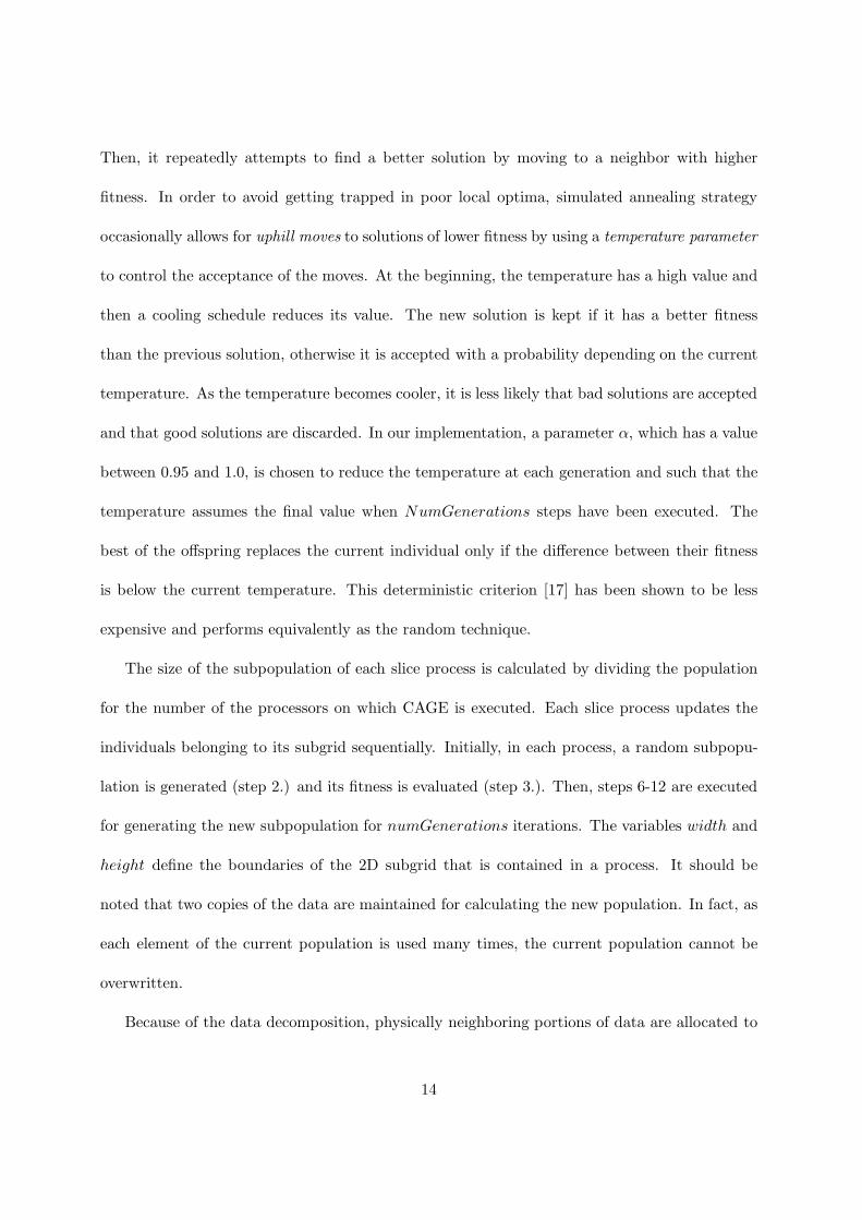
Then, it repeatedly attempts to find a better solution by moving to a neighbor with higher

fitness. In order to avoid getting trapped in poor local optima, simulated annealing strategy

occasionally allows for uphill moves to solutions of lower fitness by using a temperature parameter

to control the acceptance of the moves. At the beginning, the temperature has a high value and

then a cooling schedule reduces its value. The new solution is kept if it has a better fitness

than the previous solution, otherwise it is accepted with a probability depending on the current

temperature. As the temperature becomes cooler, it is less likely that bad solutions are accepted

and that good solutions are discarded. In our implementation, a parameter α, which has a value

between 0.95 and 1.0, is chosen to reduce the temperature at each generation and such that the

temperature assumes the final value when NumGenerations steps have been executed. The

best of the offspring replaces the current individual only if the difference between their fitness

is below the current temperature. This deterministic criterion [17] has been shown to be less

expensive and performs equivalently as the random technique.

The size of the subpopulation of each slice process is calculated by dividing the population

for the number of the processors on which CAGE is executed. Each slice process updates the

individuals belonging to its subgrid sequentially. Initially, in each process, a random subpopu-

lation is generated (step 2.) and its fitness is evaluated (step 3.). Then, steps 6-12 are executed

for generating the new subpopulation for numGenerations iterations. The variables width and

height define the boundaries of the 2D subgrid that is contained in a process. It should be

noted that two copies of the data are maintained for calculating the new population. In fact, as

each element of the current population is used many times, the current population cannot be

overwritten.

Because of the data decomposition, physically neighboring portions of data are allocated to

14

different processes. To improve the performances and to reduce the overhead due to the remote

communications, we introduced a local copy of boundary data in each process. This avoids

remote communication more than once on the same data. Boundary data are exchanged at each

iteration before breeding the new population. In our implementation, the processes form a logical

ring and each processor determines its right- and left-neighboring processes. The communication

between processes is local since only the outermost individuals need to communicate between

the slice processes.

All the communications are performed using the MPI (Message Passing Interface) portable

message passing system so that CAGE can be executed across different hardware platforms.

Since the processes are connected according to a ring architecture and each process has a lim-

ited buffer for storing boundary data, we use asynchronous communication in order to avoid

processors to idle.

Each processor has two send buffers (SRbuf, SLbuf) and two receive buffers (RRbuf ,

RLbuf). The SRbuf and SLbuf buffers correspond to the outermost (right and left) individuals

of the subgrid. The receive buffers are added to the subgrid in order to obtain a bordered

grid. The exchange of the boundary data occurs, in each process, by two asynchronous send

operations followed by two asynchronous receive operations to the right- and left-neighboring

processes. After this, each process waits until the asynchronous operations complete.

15

MPI Isend(SRbuf, right);

MPI Isend(SLbuf, left);

MPI Irecv(RRbuf, right);

MPI Irecv(RLbuf, left);

MPI Waitall();

Figure 2: Pseudocode for data movement.

16

Figure 2 shows the pseudocode for this data movement operation.

CAGE uses the standard tool for GP , sgpc1.1, a simple GP in the C language, available

freely at [36], to apply the GP algorithm to each grid point. However, in order to meet the

requirements of the cellular GP algorithm, a number of modifications were introduced.

We used the same data structure of sgpc1.1 to store a tree in each cell. The structure

that stores the population was transformed from a one-dimensional array to a two-dimensional

one and we duplicated this structure in order to store the current and the new generated tree.

The selection procedure was replaced with one that uses only the neighborhood cells and three

replacement policies were added. Crossover is performed between the current tree and the

best tree in the neighborhood. Two procedures to pack and unpack the trees, that must be

sent/received to/from the other processes, were added. The pack procedure is used to send

the trees of the boundary data to the neighboring processes in a linearized form. We use a

breadth-first traversal to linearize the trees of the boundary data into an array. However, before

exchanging the array containing the linearized trees, we send another array containing the size

of the trees to the neighboring processes in order to allow an optimized allocation of the space

in memory of the receiving nodes. Immediately after, the unpack procedure rebuilds the data

and stores them in the new processor’s private address space.

17

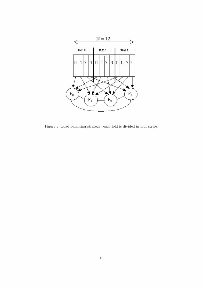
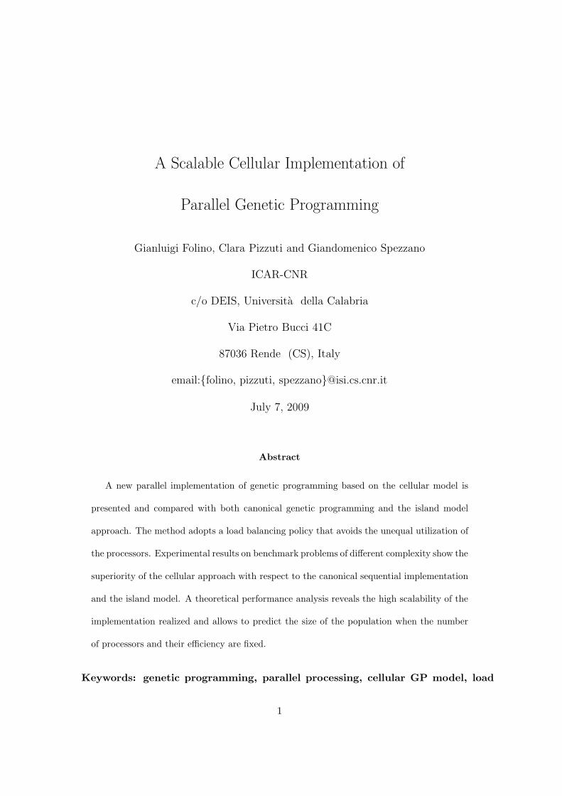
Figure 3: Load balancing strategy: each fold is divided in four strips.

18

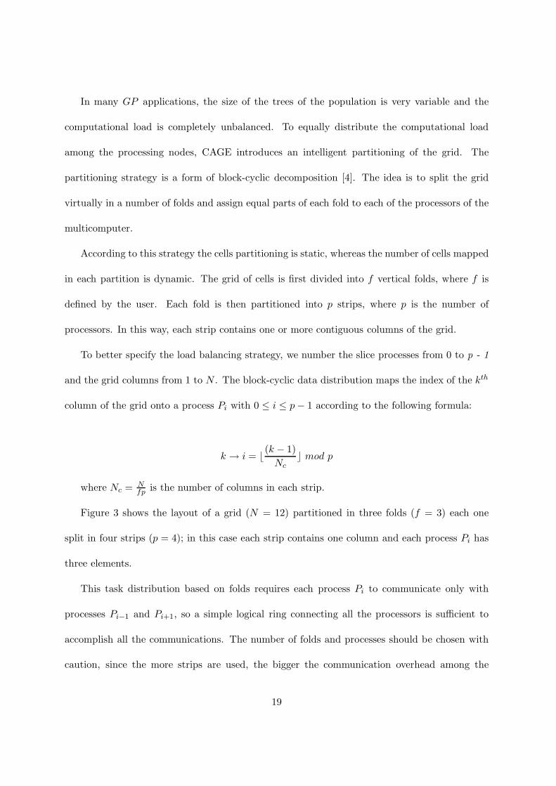
In many GP applications, the size of the trees of the population is very variable and the

computational load is completely unbalanced. To equally distribute the computational load

among the processing nodes, CAGE introduces an intelligent partitioning of the grid. The

partitioning strategy is a form of block-cyclic decomposition [4]. The idea is to split the grid

virtually in a number of folds and assign equal parts of each fold to each of the processors of the

multicomputer.

According to this strategy the cells partitioning is static, whereas the number of cells mapped

in each partition is dynamic. The grid of cells is first divided into f vertical folds, where f is

defined by the user. Each fold is then partitioned into p strips, where p is the number of

processors. In this way, each strip contains one or more contiguous columns of the grid.

To better specify the load balancing strategy, we number the slice processes from 0 to p - 1

and the grid columns from 1 to N . The block-cyclic data distribution maps the index of the kth

column of the grid onto a process Pi with 0 ≤ i ≤ p − 1 according to the following formula:

k → i = ⌊(k − 1)

Nc⌋ mod p

where Nc = Nfp

is the number of columns in each strip.

Figure 3 shows the layout of a grid (N = 12) partitioned in three folds (f = 3) each one

split in four strips (p = 4); in this case each strip contains one column and each process Pi has

three elements.

This task distribution based on folds requires each process Pi to communicate only with

processes Pi−1 and Pi+1, so a simple logical ring connecting all the processors is sufficient to

accomplish all the communications. The number of folds and processes should be chosen with

caution, since the more strips are used, the bigger the communication overhead among the

19

processing elements becomes.

The next section presents a theoretical performance analysis of CAGE. This analysis allows

us to evaluate the performance of CAGE when the population size and the number of processors

are increased. Note that the quality of the solution obtained is not related to this kind of

analysis.

5 Performance Analysis

In this section, we analyze the performance of our parallel implementation of GP . We first focus

on genetic programs in which we do not consider the effects of the load balancing algorithm.

Then we extend our model to handle the strategy of load balancing presented in the previous

section. Analyzing the performance of a given parallel algorithm/architecture requires a method

to evaluate scalability. The isoefficiency function [16] is one among many parallel performance

metrics that measure scalability. It indicates how the problem size n must grow as the num-

ber of processor m increases in order to obtain a given efficiency E. It relates problem size to

the number of processors required to maintain the efficiency of a system, and lets us to deter-

mine scalability with respect to the number of processors, their speed, and the communication

bandwidth of the interconnection network.

We assume that GP works on a population of size A × B points, where A is the width and

B is the height of the grid. Furthermore, s represents the average dimension of the trees of

the population. On a sequential machine we can model the computation time T1 for evolving a

population of genetic programs for one generation as:

T1 = tas + AB(tf + tup)

20

where tf is the average computation time required to perform the evaluation phase at a single

grid point; tas is the average time required at each generation to perform some simple operations,

such as the increment of the iterations and the zero setting of some variables; tup is the time

necessary to update, after one evaluation, the state of each cell of the grid with the new genetic

program and the corresponding value of the fitness. So, defining t′f = tf + tup we have:

T1 = tas + ABt′f (1)

The parallel execution time of the GP program on a distributed memory parallel machine with

p processors can be modelled by summing up the computation time needed to evaluate the

genetic programs on a partition A/p of the grid, the time for packing and unpacking the trees,

representing the genetic programs, and the communication time needed to exchange the buffers

containing the trees of the boundary data to the neighboring processes. Therefore, the parallel

execution time can be estimated as follows:

Tp = (tas +A

pBt′f ) + Tpack + Tunpack + Texc (2)

where Tpack is the time spent to pack each tree from its memory representation into two linearized

data structures, containing the size and the nodes of each tree respectively; Tunpack is the time

necessary to rebuild the equivalent trees in memory of the received data from the neighboring

processors, and Texc is the time required to exchange the borders.

The time for packing and unpacking is:

Tpack + Tunpack = Bs(t1 + t2) = Bstpunp (3)

where t1 is the time to visit a tree and build the linearized data structures and t2 is the time to

rebuild the tree. Let tpunp = t1 + t2. To take into account the communication time, we consider

21

that each task must exchange with two neighboring tasks the borders of its own portion and

receive those of the neighbors for a total of four messages. As we must exchange two data

structure (trees and their size), the time required to exchange the borders can be estimated,

according to Hockney’s model [18], as:

Texc = 4(ts + sBtb) + 4(ts + 4Btb) = 8ts + 4Btb(4 + s) (4)

where s is the average size of a tree, ts is the startup time, that is, the time required to initiate

the communication, and tb is the incremental transmission time per byte, which is determined

by the physical bandwidth of the communication channel linking the source and destination

processors. Therefore we can represent the parallel execution time as:

Tp = tap + B[A

pt′f + 4tb(4 + s) + stpunp] (5)

where tap = 8ts + tas + α. The α parameter includes all the times that do not depend on the

size of the grid and the communication among processors.

The overhead function T0 of a parallel system represents the total sum of all overhead incurred

by the p processors during the parallel execution of the algorithm and it depends on the problem

size. In our case T0 is given by:

T0 = pTp − T1∼= p(tap + 4Btb(4 + s) + Bstpunp) (6)

under the really plausible hypothesis that tas is negligible with respect to the total time. The

speedup on p processors can be evaluated as S = T1

Tp

and the efficiency as E = Sp. Using the

expressions 1 and 5, the speedup and the efficiency can be expressed respectively as:

S =T1

Tp

=tas + ABt′f

tap + B[Apt′f + 4tb(4 + s) + stpunp]

(7)

22

E =S

p=

tas + ABt′fABt′f + p[4Btb(4 + s) + sBtpunp + tap]

(8)

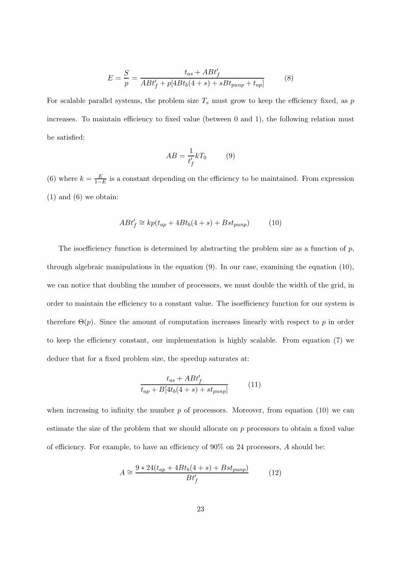
For scalable parallel systems, the problem size Ts must grow to keep the efficiency fixed, as p

increases. To maintain efficiency to fixed value (between 0 and 1), the following relation must

be satisfied:

AB =1

t′fkT0 (9)

(6) where k = E1−E

is a constant depending on the efficiency to be maintained. From expression

(1) and (6) we obtain:

ABt′f∼= kp(tap + 4Btb(4 + s) + Bstpunp) (10)

The isoefficiency function is determined by abstracting the problem size as a function of p,

through algebraic manipulations in the equation (9). In our case, examining the equation (10),

we can notice that doubling the number of processors, we must double the width of the grid, in

order to maintain the efficiency to a constant value. The isoefficiency function for our system is

therefore Θ(p). Since the amount of computation increases linearly with respect to p in order

to keep the efficiency constant, our implementation is highly scalable. From equation (7) we

deduce that for a fixed problem size, the speedup saturates at:

tas + ABt′ftap + B[4tb(4 + s) + stpunp]

(11)

when increasing to infinity the number p of processors. Moreover, from equation (10) we can

estimate the size of the problem that we should allocate on p processors to obtain a fixed value

of efficiency. For example, to have an efficiency of 90% on 24 processors, A should be:

A ∼=9 ∗ 24(tap + 4Btb(4 + s) + Bstpunp)

Bt′f(12)

23

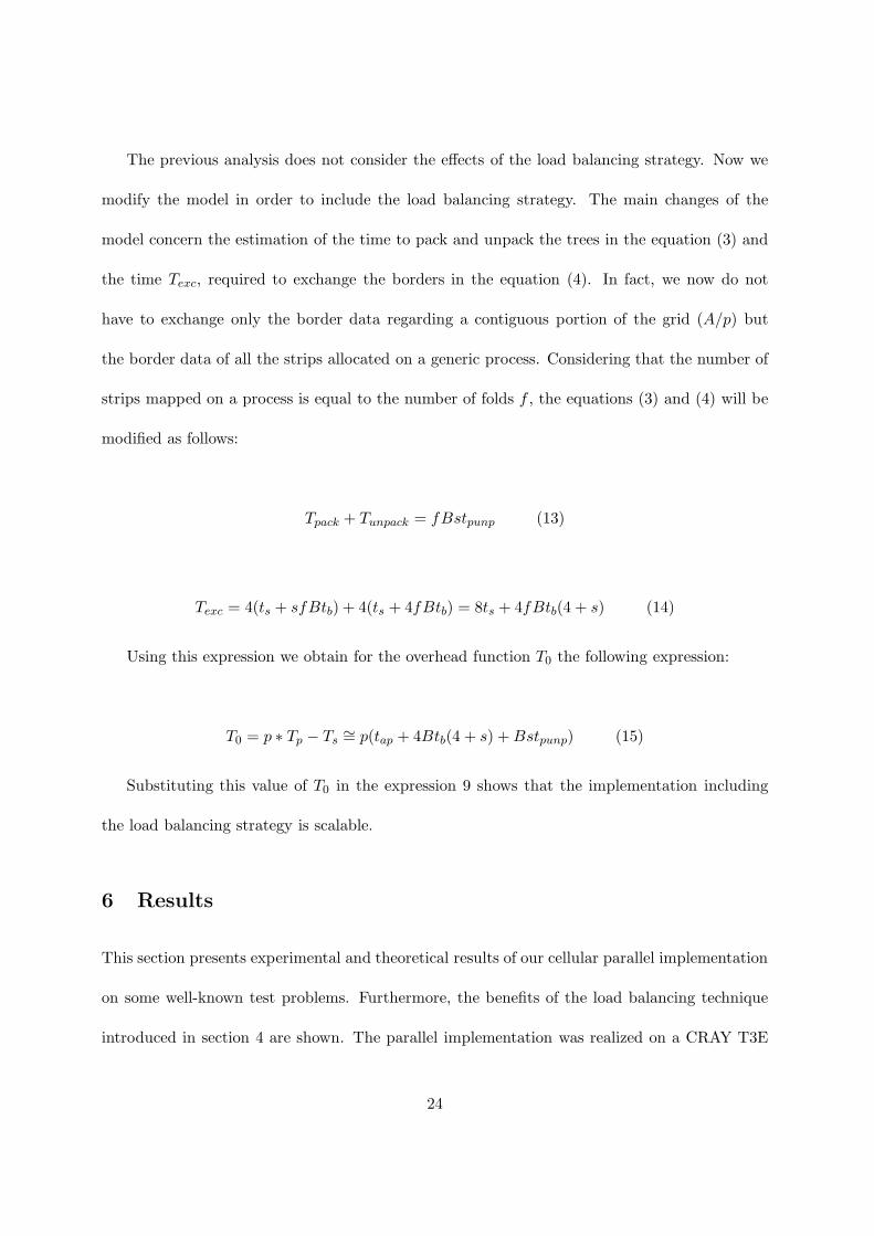
The previous analysis does not consider the effects of the load balancing strategy. Now we

modify the model in order to include the load balancing strategy. The main changes of the

model concern the estimation of the time to pack and unpack the trees in the equation (3) and

the time Texc, required to exchange the borders in the equation (4). In fact, we now do not

have to exchange only the border data regarding a contiguous portion of the grid (A/p) but

the border data of all the strips allocated on a generic process. Considering that the number of

strips mapped on a process is equal to the number of folds f , the equations (3) and (4) will be

modified as follows:

Tpack + Tunpack = fBstpunp (13)

Texc = 4(ts + sfBtb) + 4(ts + 4fBtb) = 8ts + 4fBtb(4 + s) (14)

Using this expression we obtain for the overhead function T0 the following expression:

T0 = p ∗ Tp − Ts∼= p(tap + 4Btb(4 + s) + Bstpunp) (15)

Substituting this value of T0 in the expression 9 shows that the implementation including

the load balancing strategy is scalable.

6 Results

This section presents experimental and theoretical results of our cellular parallel implementation

on some well-known test problems. Furthermore, the benefits of the load balancing technique

introduced in section 4 are shown. The parallel implementation was realized on a CRAY T3E

24

parallel machine with 256 processors based on DEC Alpha processor with 128 Mbytes of memory.

We used sgpc1.1 [36] as the sequential implementation of genetic programming.

6.1 Experimental Analysis

This subsection presents a detailed description of each test problem. The convergence results

obtained with CAGE when the greedy replacement policy was adopted are compared with

sequential GP . We also present the convergence behavior of CAGE when the direct, greedy,

and probabilistic replacement policies were used and the influence of the population size on the

convergence of the method. The parameters of the method are shown in table 1 and functions

and terminal symbols for each problem are described in table 2. Each problem was run 20 times

for 100 generations. For all the experiments, we used the Moore neighborhood and a population

size of 3200, except for Symbolic Regression. For this problem, the size of the population was

800 individuals.

25

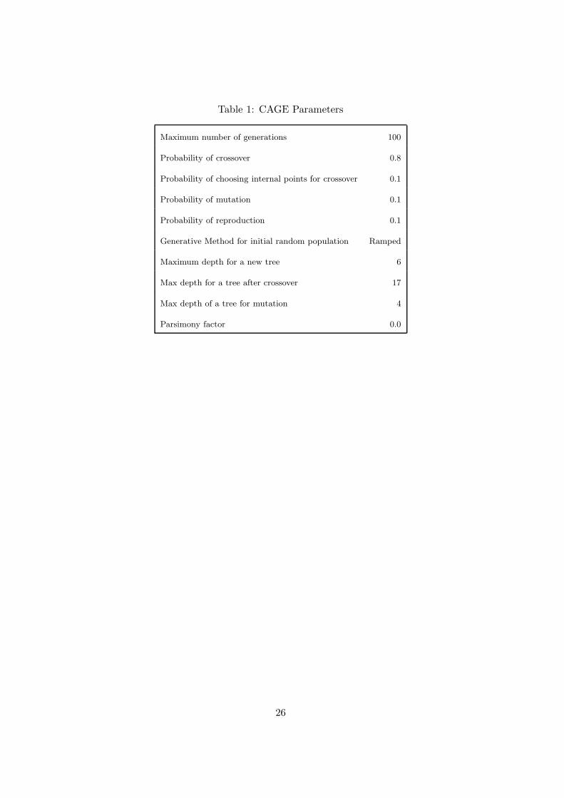
Table 1: CAGE Parameters

Maximum number of generations 100

Probability of crossover 0.8

Probability of choosing internal points for crossover 0.1

Probability of mutation 0.1

Probability of reproduction 0.1

Generative Method for initial random population Ramped

Maximum depth for a new tree 6

Max depth for a tree after crossover 17

Max depth of a tree for mutation 4

Parsimony factor 0.0

26

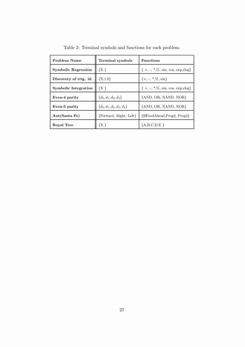
Table 2: Terminal symbols and functions for each problem.

Problem Name Terminal symbols Functions

Symbolic Regression {X } { +, -, *,%, sin, cos, exp,rlog}

Discovery of trig. id. {X,1.0} {+, -, *,%, sin}

Symbolic Integration {X } { +, -, *,%, sin, cos, exp,rlog}

Even-4 parity {d0, d1, d2, d3} {AND, OR, NAND, NOR}

Even-5 parity {d0, d1, d2, d3, d4} {AND, OR, NAND, NOR}

Ant(Santa Fe) {Forward, Right, Left} {IfFoodAhead,Prog2, Prog3}

Royal Tree {X } {A,B,C,D,E }

27

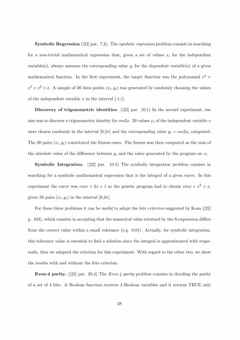
Symbolic Regression ([22] par. 7.3). The symbolic regression problem consists in searching

for a non-trivial mathematical expression that, given a set of values xi for the independent

variable(s), always assumes the corresponding value yi for the dependent variable(s) of a given

mathematical function. In the first experiment, the target function was the polynomial x4 +

x3 + x2 + x. A sample of 20 data points (xi, yi) was generated by randomly choosing the values

of the independent variable x in the interval [-1,1].

Discovery of trigonometric identities. ([22] par. 10.1) In the second experiment, our

aim was to discover a trigonometric identity for cos2x. 20 values xi of the independent variable x

were chosen randomly in the interval [0,2π] and the corresponding value yi = cos2xi computed.

The 20 pairs (xi, yi) constituted the fitness cases. The fitness was then computed as the sum of

the absolute value of the difference between yi and the value generated by the program on xi.

Symbolic Integration. ([22] par. 10.5) The symbolic integration problem consists in

searching for a symbolic mathematical expression that is the integral of a given curve. In this

experiment the curve was cosx + 2x + 1 so the genetic program had to obtain sinx + x2 + x,

given 50 pairs (xi, yi) in the interval [0,2π].

For these three problems it can be useful to adopt the hits criterion suggested by Koza ([22]

p. 163), which consists in accepting that the numerical value returned by the S-expression differs

from the correct value within a small tolerance (e.g. 0.01). Actually, for symbolic integration,

this tolerance value is essential to find a solution since the integral is approximated with trape-

zoids, thus we adopted the criterion for this experiment. With regard to the other two, we show

the results with and without the hits criterion.

Even-4 parity. ([22] par. 20.4) The Even-4 parity problem consists in deciding the parity

of a set of 4 bits. A Boolean function receives 4 Boolean variables and it returns TRUE only

28

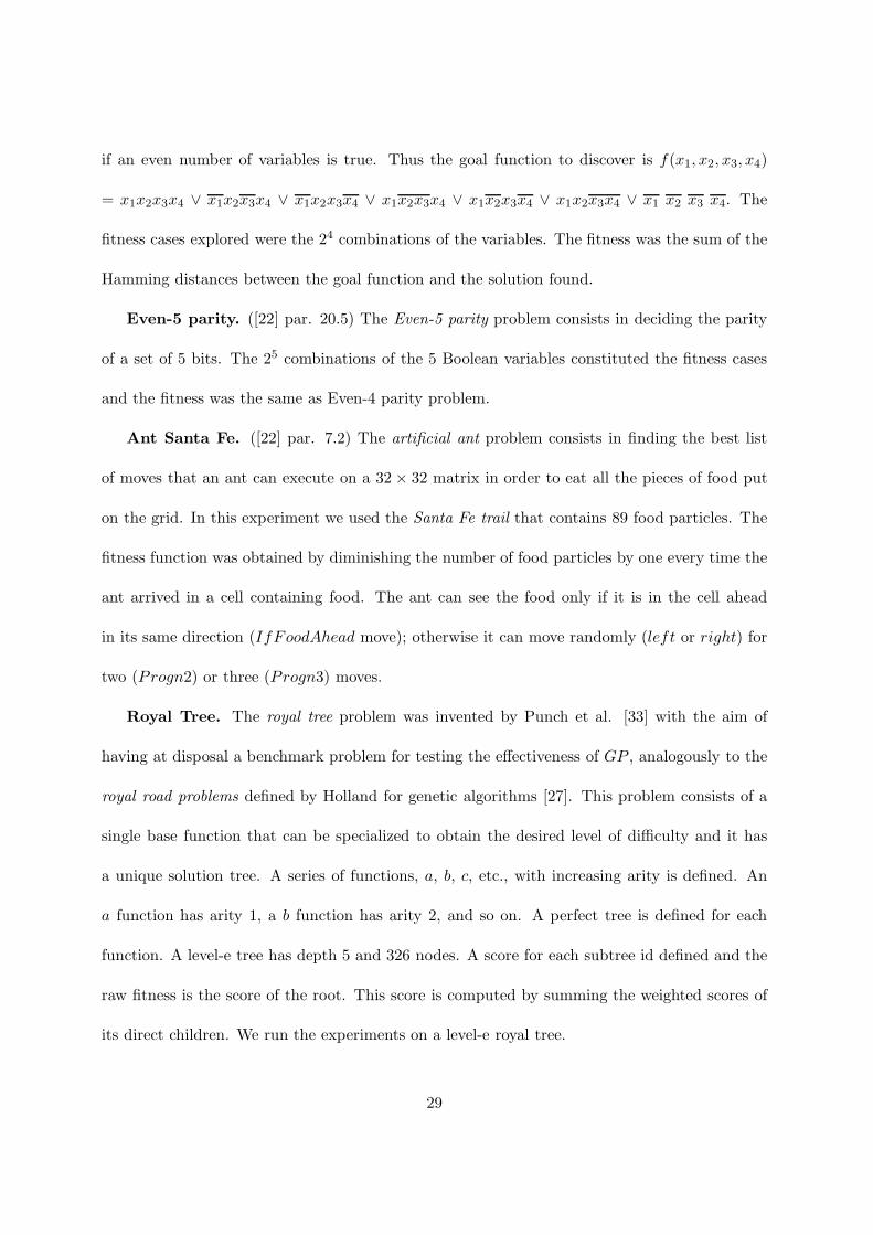
if an even number of variables is true. Thus the goal function to discover is f(x1, x2, x3, x4)

= x1x2x3x4 ∨ x1x2x3x4 ∨ x1x2x3x4 ∨ x1x2x3x4 ∨ x1x2x3x4 ∨ x1x2x3x4 ∨ x1 x2 x3 x4. The

fitness cases explored were the 24 combinations of the variables. The fitness was the sum of the

Hamming distances between the goal function and the solution found.

Even-5 parity. ([22] par. 20.5) The Even-5 parity problem consists in deciding the parity

of a set of 5 bits. The 25 combinations of the 5 Boolean variables constituted the fitness cases

and the fitness was the same as Even-4 parity problem.

Ant Santa Fe. ([22] par. 7.2) The artificial ant problem consists in finding the best list

of moves that an ant can execute on a 32 × 32 matrix in order to eat all the pieces of food put

on the grid. In this experiment we used the Santa Fe trail that contains 89 food particles. The

fitness function was obtained by diminishing the number of food particles by one every time the

ant arrived in a cell containing food. The ant can see the food only if it is in the cell ahead

in its same direction (IfFoodAhead move); otherwise it can move randomly (left or right) for

two (Progn2) or three (Progn3) moves.

Royal Tree. The royal tree problem was invented by Punch et al. [33] with the aim of

having at disposal a benchmark problem for testing the effectiveness of GP , analogously to the

royal road problems defined by Holland for genetic algorithms [27]. This problem consists of a

single base function that can be specialized to obtain the desired level of difficulty and it has

a unique solution tree. A series of functions, a, b, c, etc., with increasing arity is defined. An

a function has arity 1, a b function has arity 2, and so on. A perfect tree is defined for each

function. A level-e tree has depth 5 and 326 nodes. A score for each subtree id defined and the

raw fitness is the score of the root. This score is computed by summing the weighted scores of

its direct children. We run the experiments on a level-e royal tree.

29

These two last problems are known to be purposely difficult for distributed GP . Next, for

each of the above problems, experimental results are reported and discussed. Besides the figures

that show the convergence results, we adopted the same method of Punch [32] to present the

results of the experiments as the number of Wins and Losses obtained by running canonical

GP and CAGE for 20 times. The wins are denoted as W : (x, y), where x represents the number

of optimal solutions found before 100 generations and y the average generation in which the

optimal solution was found. The losses are denoted as L : (q, r, s), where q is the number of

losses (no optimal solution found before 100 generations) r is the average best-of-run fitness,

and s is the average generation when the best-of-run occurred. Tables 3 and 4 summarize all

the experiments.

30

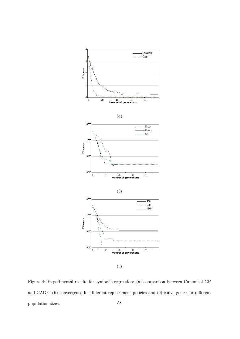
Figure 4 shows the results for symbolic regression. In particular, in figure 4(a) the comparison

between the convergence of canonical sequential GP and CAGE is presented. CAGE reaches a

good fitness value more rapidly than canonical GP and it obtains the exact solution in 18 out of

the 20 runs at, approximately, the 11th generation, while canonical GP finds the solution in 11

runs at the 42th generation. If we introduce the hits criterion (0.01), the results do not change

for either method. This behavior is expected since when the methods fail, the average fitness

is 0.25 for CAGE, and 0.52 for canonical GP. Figure 4(b) shows the CAGE behavior when the

three replacement policies are used. The greedy and probabilistic policies are similar. In figures

4(b) and (c) a logarithmic scale is used for a better view of the fitness values. Figure 4(c) shows

the influence of the population size on the convergence of the method. It is clear that the bigger

is the population the faster is the convergence.

31

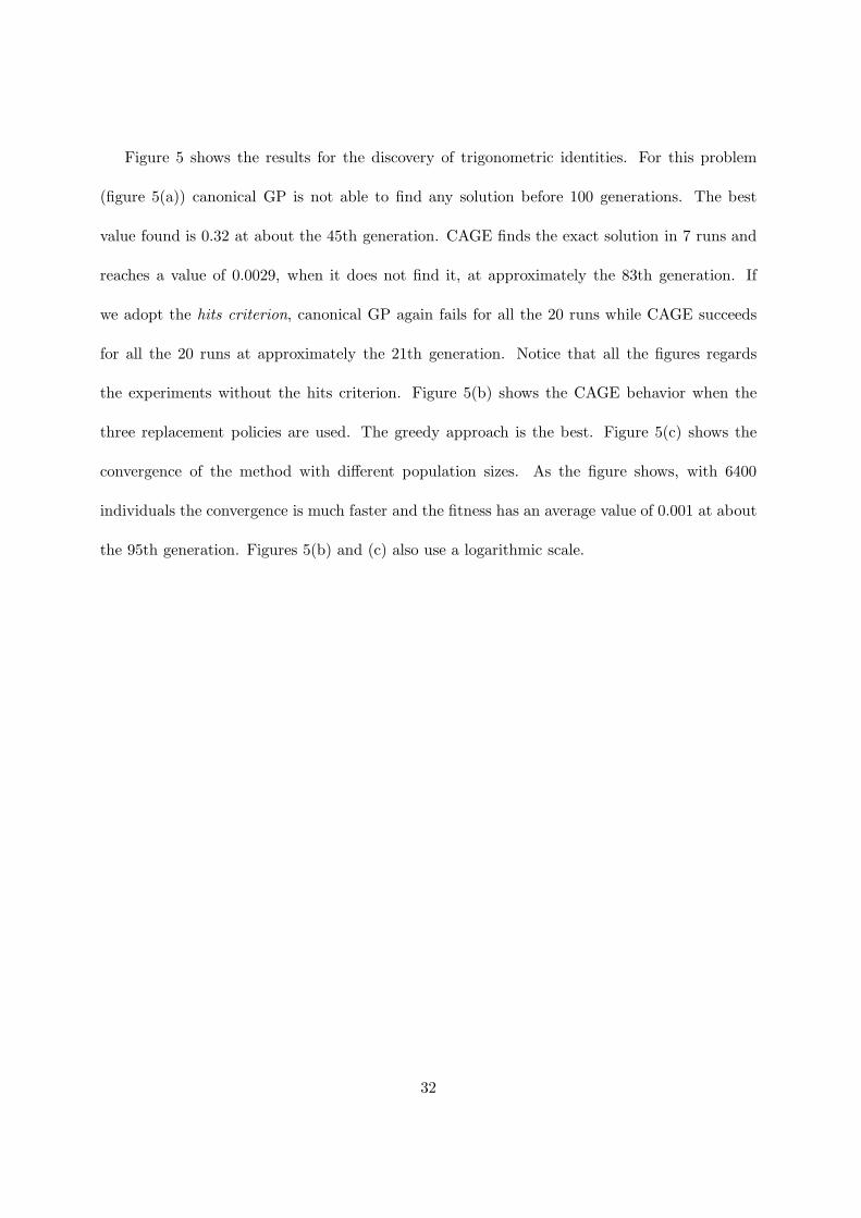
Figure 5 shows the results for the discovery of trigonometric identities. For this problem

(figure 5(a)) canonical GP is not able to find any solution before 100 generations. The best

value found is 0.32 at about the 45th generation. CAGE finds the exact solution in 7 runs and

reaches a value of 0.0029, when it does not find it, at approximately the 83th generation. If

we adopt the hits criterion, canonical GP again fails for all the 20 runs while CAGE succeeds

for all the 20 runs at approximately the 21th generation. Notice that all the figures regards

the experiments without the hits criterion. Figure 5(b) shows the CAGE behavior when the

three replacement policies are used. The greedy approach is the best. Figure 5(c) shows the

convergence of the method with different population sizes. As the figure shows, with 6400

individuals the convergence is much faster and the fitness has an average value of 0.001 at about

the 95th generation. Figures 5(b) and (c) also use a logarithmic scale.

32

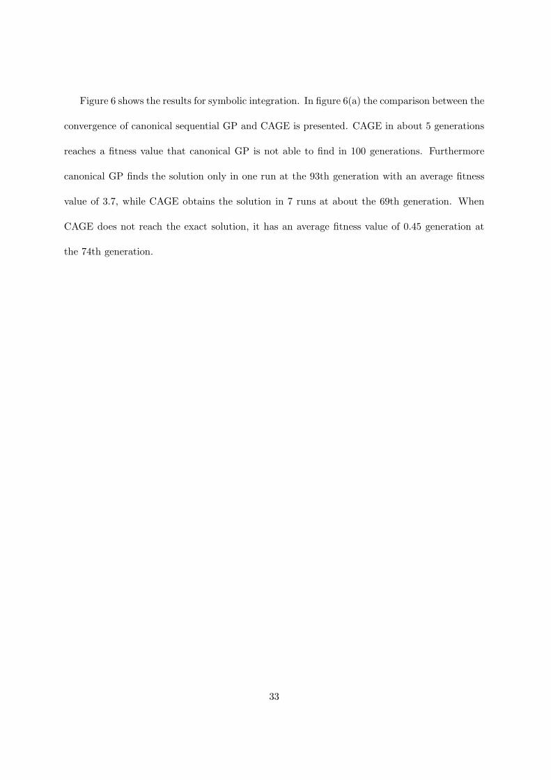
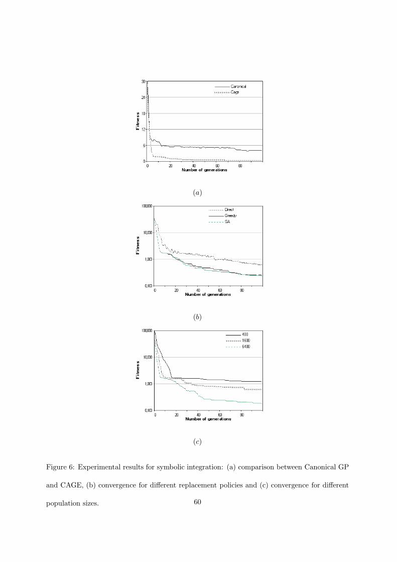
Figure 6 shows the results for symbolic integration. In figure 6(a) the comparison between the

convergence of canonical sequential GP and CAGE is presented. CAGE in about 5 generations

reaches a fitness value that canonical GP is not able to find in 100 generations. Furthermore

canonical GP finds the solution only in one run at the 93th generation with an average fitness

value of 3.7, while CAGE obtains the solution in 7 runs at about the 69th generation. When

CAGE does not reach the exact solution, it has an average fitness value of 0.45 generation at

the 74th generation.

33

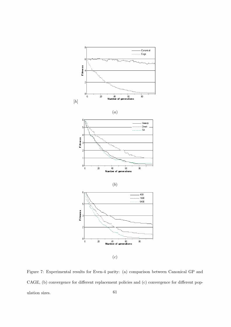
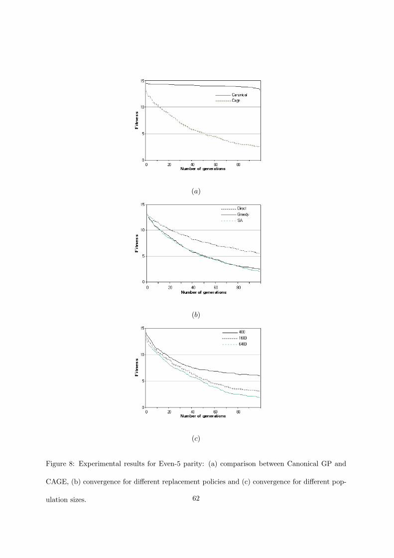
Figures 7 and 8 reports the results for Even-4 and Even-5 problems. It is well known that

this family of problems is very difficult. Koza [22] (p.532) states that when Even-5 was run with

a population of 4000 individuals for 51 generations no solution was found after 20 runs. It was

necessary to double the population to have a solution at the eighth run. With our parameters,

canonical GP could not find any solution for both Even-4 and Even-5. CAGE, on the contrary,

obtained the solution in 17 out of 20 runs for Even-4 and it was successful in two runs for

Even-5. This behavior is evident from the figures 7(a) and 8(a). Canonical GP obtained a

fitness value that is far from the solution and it was not able to appreciably improve it before

the 100th generation. CAGE did not find the solution in only two cases for Even-4. For Even-5

it obtained the solution in two runs but, when it failed to find it, the average best-of-run fitness

was very low. Figure 8(c) shows the convergence improvement when populations of increasing

sizes are used. For instance, when CAGE ran with a population of 6400 individuals, at the

100th generation the average fitness wass 1.77, while with 1600 individuals it was 3.10.

34

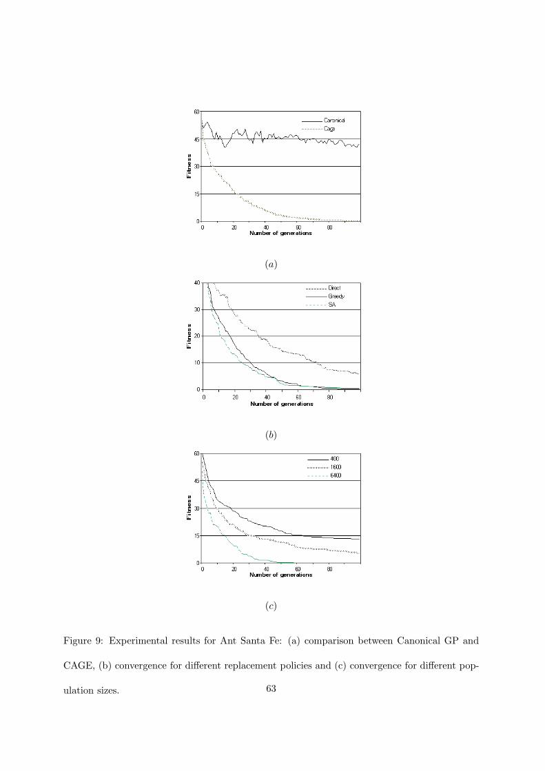
In figure 9 the convergence results of CAGE with respect to canonical GP are shown for the

Ant Santa Fe problem. The figure clearly points out that, after 100 generations, canonical GP

is far from the solution, while CAGE failed only once in finding the solution. By doubling the

population the convergence is much faster and CAGE always succeeded before an average of 55

generations. Also for the Royal tree problem (figure 10(a)) canonical GP always failed, while

CAGE obtains the solution for all the 20 runs at, approximately, the 78th generation. Figure

10(c) shows the convergence when 800, 1600 and 3200 individuals are used and it clearly points

out that, by increasing the population size, the method has a better convergence.

35

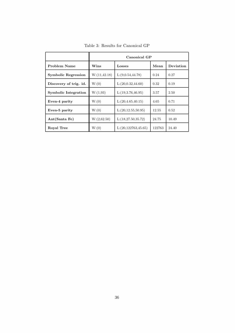
Table 3: Results for Canonical GP

Canonical GP

Problem Name Wins Losses Mean Deviation

Symbolic Regression W:(11,42.18) L:(9,0.54,44.78) 0.24 0.27

Discovery of trig. id. W:(0) L:(20,0.32,44.60) 0.32 0.19

Symbolic Integration W:(1,93) L:(19,3.76,46.95) 3.57 2.50

Even-4 parity W:(0) L:(20,4.65,40.15) 4.65 0.71

Even-5 parity W:(0) L:(20,12.55,50.95) 12.55 0.52

Ant(Santa Fe) W:(2,62.50) L:(18,27.50,35.72) 24.75 10.49

Royal Tree W:(0) L:(20,122763,45.65) 122763 24.40

36

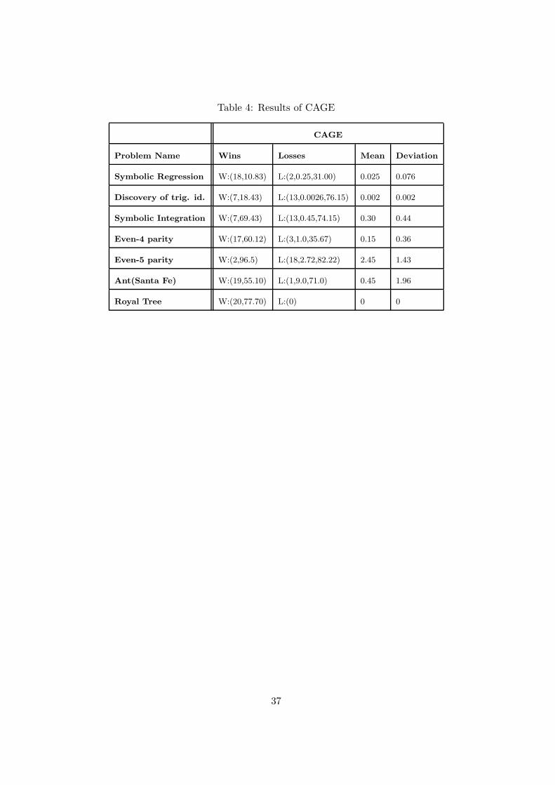
Table 4: Results of CAGE

CAGE

Problem Name Wins Losses Mean Deviation

Symbolic Regression W:(18,10.83) L:(2,0.25,31.00) 0.025 0.076

Discovery of trig. id. W:(7,18.43) L:(13,0.0026,76.15) 0.002 0.002

Symbolic Integration W:(7,69.43) L:(13,0.45,74.15) 0.30 0.44

Even-4 parity W:(17,60.12) L:(3,1.0,35.67) 0.15 0.36

Even-5 parity W:(2,96.5) L:(18,2.72,82.22) 2.45 1.43

Ant(Santa Fe) W:(19,55.10) L:(1,9.0,71.0) 0.45 1.96

Royal Tree W:(20,77.70) L:(0) 0 0

37

For all the seven problems CAGE outperformed canonical GP . This result allows us to state

that the parallel cellular genetic programming implementation, analogously to parallel genetic

algorithms [37], needed fewer evaluations to get the same solution quality than for the single

population case with the same total number of individuals.

6.2 Experimental performance evaluation

To illustrate the use of our scalability prediction technique and to assess its accuracy, we present

two examples: the Even-4 parity problem and the Ant problem. For both problems we considered

a population of 128x13 cells.

38

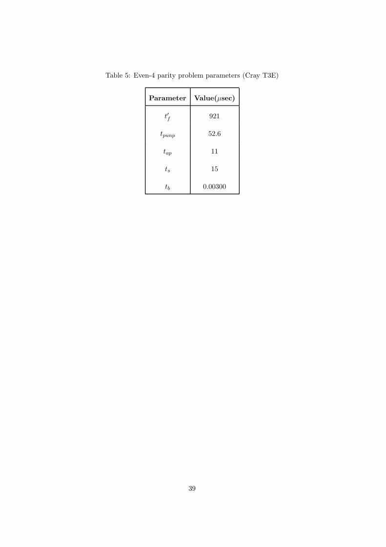
Table 5: Even-4 parity problem parameters (Cray T3E)

Parameter Value(µsec)

t′f 921

tpunp 52.6

tap 11

ts 15

tb 0.00300

39

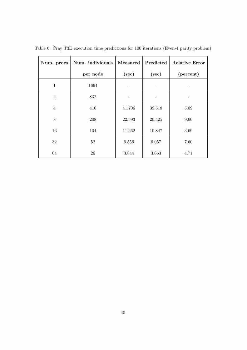
Table 6: Cray T3E execution time predictions for 100 iterations (Even-4 parity problem)

Num. procs Num. individuals Measured Predicted Relative Error

per node (sec) (sec) (percent)

1 1664 - - -

2 832 - - -

4 416 41.706 39.518 5.09

8 208 22.593 20.425 9.60

16 104 11.262 10.847 3.69

32 52 6.556 6.057 7.60

64 26 3.844 3.663 4.71

40

Table 5 shows, for the Even-4 parity problem, the estimated values of the parameters neces-

sary to evaluate the parallel execution time Tp for different number of processors using equation

(2). The t′f value was estimated by measuring its computational cost for different problem sizes

(i.e. changing the A value) and then using the Matlab toolkit to automatically calculate the

least-squares fit of the equation that defines t′f with the experimental data. Likewise, we es-

timated tpunp. tap was estimated by measuring its computational cost for different number of

processors and then calculating the least-squares fit of the equation that defines tap with the

experimental data. The ts and tb values for the CRAY T3E machine were estimated as already

done in a previous work for a Meiko CS-2 machine [14]. The average size s of the trees was

18.35 nodes. Table 6 shows the measured and predicted execution times, and the relative error

associated with each prediction for the Even-4 problem.

41

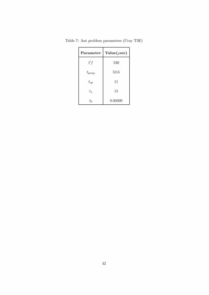
Table 7: Ant problem parameters (Cray T3E)

Parameter Value(µsec)

t′f 530

tpunp 52.6

tap 11

ts 15

tb 0.00300

42

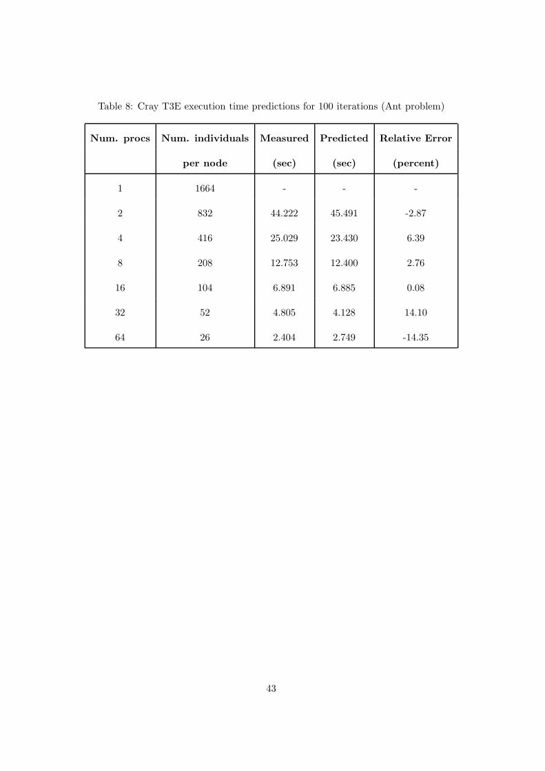
Table 8: Cray T3E execution time predictions for 100 iterations (Ant problem)

Num. procs Num. individuals Measured Predicted Relative Error

per node (sec) (sec) (percent)

1 1664 - - -

2 832 44.222 45.491 -2.87

4 416 25.029 23.430 6.39

8 208 12.753 12.400 2.76

16 104 6.891 6.885 0.08

32 52 4.805 4.128 14.10

64 26 2.404 2.749 -14.35

43

For the Ant problem, the average size s of the trees was 19.84 nodes and the values of

the constants to evaluate Tp are shown in table 7. Table 8 shows the measured and predicted

execution times, and the relative error associated with each prediction for the Ant problem.

The results described in tables 6 and 8 show a good agreement between the model and

the experiments. In fact, for the Even-4 problem the measured times were, on average, 6%

off the predicted and, on average, 7% off for the Ant problem. The relative error is smaller

in the second example because the computation component of the model dominates. Since

it is the most accurately estimated model term, the prediction becomes increasingly accurate

with larger problems. A more accurate prediction model is obtainable using a refined model of

communication cost [15].

From equation 8, we calculate that the value of the speedup is bound to 122.02 for the Even-4

problem and to 64.9 for the Ant problem. The lower value of speedup for the Ant problem is

due to the much larger communication/computation ratio. In fact, the average computation

time, required to perform the evaluation phase at a single grid point in the Ant problem, is

about the half of the time required for the Even-4 problem. We can obtain a better value of

speedup increasing the granularity, that is, allocating a larger number of cells for node. We can

use formula 7 to calculate the exact size of A to increase the speedup. For example, from this

formula, we obtain a size of A equal to 1135 to have an efficiency of 90% on 64 processors. The

model can be helpful to calculate the correct size of the population of the GP in order to obtain

a given efficiency for a specific architecture. Furthermore, we can determinate, for a specific

population, the optimal number of processors that allow reaching a specific efficiency.

44

6.3 Evaluation of the load balancing strategy

This subsection briefly presents some results concerning the load balancing strategy proposed

in section 4. Before implementing the strategy we have analyzed the size of the trees of the

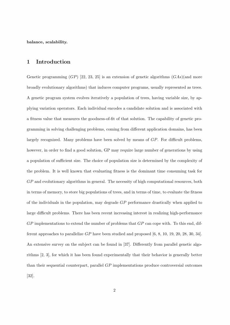
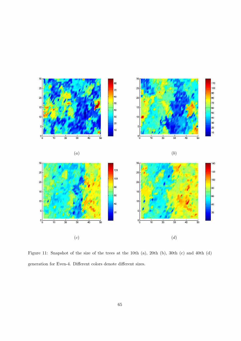
population for different problems and iterations. Figure 11 shows a snapshot of the size of the

trees for different iterations (namely 10th, 20th, 30th and 40th) for the Even-4 problem, using

a 50 x 30 grid. The size of the trees is very variable and the computational load is completely

unbalanced. This behavior is similar for many of the problems used in our analysis. We have

implemented and tested the load balancing strategy for all the problems of our test suite. A

complete description of the results is presented in [13]. 20 % improvement on average has

been obtained for the most of the problems. This result confirms the importance of a load

balancing strategy for parallel GP implementations in order to avoid an inefficient utilization of

the processors. Note that all the experiments presented in the previous subsection were obtained

without load balancing.

45

7 Comparison with the island model

This section compares the results presented by Niwa and Iba [28], those reported by Punch [32],

and by Fernandez et al. [8], with those obtained by CAGE. To compare our method with these

other island-model implementations, we ran CAGE with the same parameters of each approach.

However, since we did not run their software, a number of details could be different and influence

the quality of the results. For example, Punch used the lilgp package [33], while Fernandez et

al. used the GPC++ package [40].

46

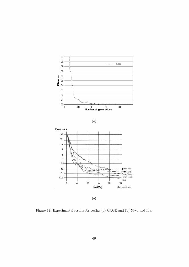
Figures 12(a) and (b) report the results obtained by CAGE and by Niwa and Iba [28] for the

discovery of trigonometric identities problem. In figure 12(a), for a better view of the results,

the fitness is displayed when it assumes values between 0 and 1. Figure 12(b) was obtained by

scanning the figure in [28]. With regard to this problem, the better implementation Niwa and

Iba obtained (ring topology) gives a fitness value of 0.5 at the 20th generation, of 0.2 at about

the 30th, and 0.1 at about the 62th. CAGE, instead, obtained a fitness value of 0.5 at the 10th

generation, of 0.2 at about the 15th, and 0.1 at the 20th. We do not know how many wins and

losses they had.

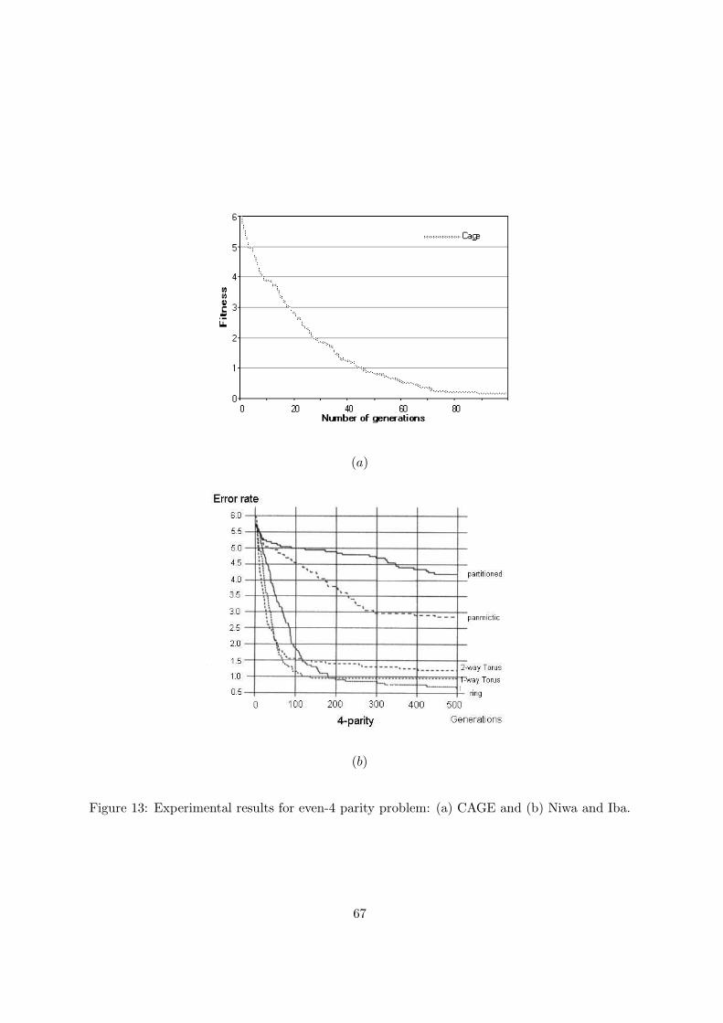
Figures 13(a) and (b) show the results obtained by CAGE and by Niwa and Iba [28] for the

Even-4 parity problem. For this problem, Niwa and Iba do not always find the correct Boolean

function not even after 500 generations. CAGE fails in only three runs before 100 generations

with an average best-of-run fitness of 1 at the average generation 36 when the best-of-run

occurred. Unfortunately we do not have these kind of details with regard to the implementation

of Niwa and Iba. At the 100th generation, their average fitness value is about 1.1.

47

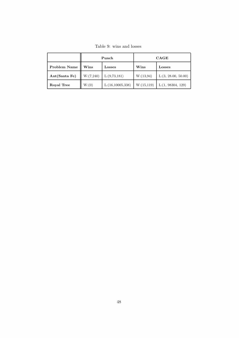
Table 9: wins and losses

Punch CAGE

Problem Name Wins Losses Wins Losses

Ant(Santa Fe) W:(7,240) L:(9,73,181) W:(13,94) L:(3, 28.00, 50.00)

Royal Tree W:(0) L:(16,10005,338) W:(15,119) L:(1, 98304, 129)

48

To compare our results with those of Punch [32], we computed the wins and losses for the ant

and royal tree problems by running CAGE the same number of times (16) as Punch reported,

the same population size (1000) and for 500 generations. Punch obtained the best result for

the ant problem by using a ring of 5 populations with proportional selection and no mutation,

while for the royal tree with over selection and no mutation. Table 9 compares these results with

CAGE’s and it confirms the better performances of CAGE with respect to the island approach.

The single-population results that Punch obtained by using the GP tool lilgp [33] are better

than the multi-population results for these two problems. The best results of his canonical GP

are W : (10, 109) and L : (6, 73, 300) for the ant problem and W : (8, 233), L : (8, 9064, 159) for

the royal tree problem. Even compared with these results, CAGE performed better.

49

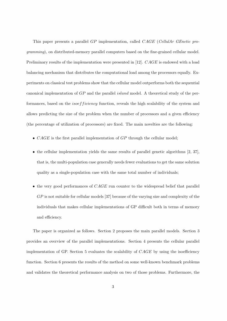
Finally we compared CAGE results for the Even-5 parity problem with those obtained by

Fernandez et al. [8], which introduced the computational effort as a measure to compare results

of the same problem. The computational effort is the number of nodes that are evaluated in

a GP tree. Let N and I be the number of times an experiment has been executed and the

number of individuals of the population, respectively. Furthermore let AV G LENGTH be the

average number of nodes per individual. Then the required effort in a particular generation is

I × N × AV G LENGTH. Figure 14 shows the effort required by CAGE. An effort equal to 7

million is required to reach a fitness value of about 24. In [8], with the same effort, the fitness

value is about 11. Thus CAGE requires fewer evaluations.

8 Conclusions

A fine-grained parallel implementation of GP through cellular model on distributed-memory

parallel computers, has been presented. Experimental results showed very good performances

of the proposed approach. The experimental study on a variety of benchmark problems has

substantiated the validity of the cellular implementation over both the island model and the

sequential single-population approach. The implementation of a load balancing strategy allows

CAGE a very good utilization of the computing resources. Finally, a theoretical performance

analysis based on the isoefficiency function permitted us to classify CAGE as a highly scalable

system and to predict execution time, speedup, and efficiency.

References

[1] D. Andre and J. R. Koza. Exploiting the fruits of parallelism: An implementation of parallel

genetic programming that achieves super-linear performance. Information Science Journal,

50

1997.

[2] E. Cantu-Paz. A summary of research on parallel genetic algorithms. Technical Report

95007, Department of General Engineering, University of Illinois at Urbana-Champaign,

Urbana, IL, 1999.

[3] E. Cantu-Paz. Efficient and Accurate Parallel Genetic Algorithms (Genetic Algorithms and

Evolutionary Computation 1). Kluwer Academic Publishers, 2000.

[4] J. J. Dongarra and P. Petitet. Algorithmic redistribution methods for block-cyclic de-

compositions. IEEE Transactions on Parallel and Distributed Systems, 10(12):1201–1216,

1999.

[5] D. C. Dracopoulos and S. Kent. Bulk synchronous parallelisation of genetic programming.

In Jerzy Wasniewski, editor, Applied parallel computing : industrial strength computation

and optimization ; Proceedings of the third International Workshop, PARA ’96, pages 216–

226, Berlin, Germany, 1996. Springer Verlag.

[6] D. C. Dracopoulos and S. Kent. Speeding up genetic programming: A parallel BSP imple-

mentation. In John R. Koza, David E. Goldberg, David B. Fogel, and Rick L. Riolo, editors,

Genetic Programming 1996: Proceedings of the First Annual Conference, pages 125–136,

Stanford University, CA, USA, 28–31 July 1996. MIT Press.

[7] F. Fernandez, J. M. Sanchez, M. Tomassini, and J. A. Gomez. A parallel genetic pro-

gramming tool based on pvm. In J. Dongarra, E. Luque, and T. Margalef, editors, Recent

Advances in Parallel Virtual Machine and Message Passing Interface, Proceedings of the

6th European PVM/MPI Users’ Group Meeting, Barcelona, Spain, September 1999, num-

51

ber 1697 in Lecture Notes in Computer Science, pages 241–248. Springer-Verlag, September

1999.

[8] F. Fernandez, M. Tomassini, W. F. Punch III, and J. M. Sanchez. Experimental study

of multipopulation parallel genetic programming. In Riccardo Poli, Wolfgang Banzhaf,

William B. Langdon, Julian F. Miller, Peter Nordin, and Terence C. Fogarty, editors,

Proceedings of EuroGP’2000, volume 1802 of LNCS, pages 283–293, Edinburgh, 15-16 April

2000. Springer-Verlag.

[9] F. Fernandez, M. Tomassini, and L. Vanneschi. Studying the influence of communication

topology and migration on distributed genetic programming. In Julian F. Miller, Marco

Tomassini, Pier Luca Lanzi, Conor Ryan, Andrea G. B. Tettamanzi, and William B. Lang-

don, editors, Proceedings of EuroGP’2001, volume 2038 of LNCS, pages 51–63, Lake Como,

Italy, 18-20 April 2001. Springer-Verlag.

[10] F. Fernandez, M. Tomassini, L. Vanneschi, and L. Bucher. A distributed computing envi-

ronment for genetic programming using mpi. In J. J. Dongarra, Peter Kacsuk, and Norbert

Podhorszki, editors, Recent advances in parallel virtual machine and message passing inter-

face: 7th European PVM/MPI Users’ Group Meeting, Balatonfured, Hungary, September

10–13, volume 1908 of Lecture Notes in Computer Science, pages 322–329, New York, NY,

USA, 2000. Springer-Verlag Inc.

[11] G. Folino, C. Pizzuti, and G. Spezzano. Genetic programming and simulated annealing: A

hybrid method to evolve decision trees. In Riccardo Poli, Wolfgang Banzhaf, William B.

Langdon, Julian Miller, Peter Nordin, and Terence C. Fogarty, editors, Proceedings of

52

EuroGP’2000, volume 1802 of LNCS, pages 294–303, Edinburgh, UK, 15-16 April 2000.

Springer-Verlag.

[12] G. Folino, C. Pizzuti, and G. Spezzano. Cage: A tool for parallel genetic programming

applications. In Julian F. Miller, Marco Tomassini, Pier Luca Lanzi, Conor Ryan, Andrea

G. B. Tettamanzi, and William B. Langdon, editors, Proceedings of EuroGP’2001, volume

2038 of LNCS, pages 64–73, Lake Como, Italy, 18-20 April 2001. Springer-Verlag.

[13] G. Folino, C. Pizzuti, and G. Spezzano. Performance evaluation of parallel genetic pro-

gramming. Technical Report 10, ISI-CNR, 2001.

[14] G. Folino, G. Spezzano, and D. Talia. Performance evaluation and modelling of mpi com-

munications on the meiko cs-2. In P. Sloot, M. Bubak, and B. Hertzberger, editors, High

Performance Computing and Networking, volume 1401 of LNCS, pages 932–936. Springer-

Verlag, 1998.

[15] I. Foster. Designing and Building Parallel Programs. Addison-Wesley, 1995.

[16] A. Y. Grama, A. Gupta, and V. Kumar. Isoefficiency: measuring the scalability of par-

allel algorithms and architectures. IEEE parallel and distributed technology: systems and

applications, 1(3):12–21, August 1993.

[17] H.Chen, N.S.Flann, and D.W.Watson. Parallel genetic simulated annealing: A massively

parallel simd algorithm. IEEE Transaction on Parallel and Distributed Systems, 9(2):126–

136, February 1998.

[18] R. W. Hockney. The communication challenge for mpp: Intel paragon and meiko cs-2.

Parallel Computing, 20(3):389–398, March 1994.

53

[19] H. Juille and J. B. Pollack. Parallel genetic programming and fine-grained SIMD architec-

ture. In E. V. Siegel and J. R. Koza, editors, Working Notes for the AAAI Symposium on

Genetic Programming, pages 31–37, MIT, Cambridge, MA, USA, 10–12 November 1995.

AAAI.

[20] H. Juille and J. B. Pollack. Massively parallel genetic programming. In Peter J. Angeline

and K. E. Kinnear, Jr., editors, Advances in Genetic Programming 2, chapter 17, pages

339–358. MIT Press, Cambridge, MA, USA, 1996.

[21] S. Kirkpatrick, C. D. Gellant, and M. P. Vecchi. Optimization by simulated annealing.

Science, (220):671–680, 1983.

[22] J. R. Koza. Genetic Programming: On the Programming of Computers by means of Natural

Selection. MIT Press, Cambridge, MA, 1992.

[23] J. R. Koza. Genetic Programming II. MIT Press, Cambridge, MA, 1994.

[24] J. R. Koza and D. Andre. Parallel genetic programming on a network of transputers.

Technical Report CS-TR-95-1542, Stanford University, Department of Computer Science,

January 1995.

[25] J. R. Koza, D. Andre, Bennett III Forrest H, and M. Keane. Genetic Programming 3:

Darwinian Invention and Problem Solving. Morgan Kaufman, 1999.

[26] W. N. Martin, J. Lienig, and J. P. Cohoon. Island (migration) models: evolutionary al-

gorithms based on punctuated equilibria. In Thomas Back, David B. Fogel, and Zbigniew

Michalewicz, editors, Handbook of Evolutionary Computation, pages C6.3:1–16. Institute of

Physics Publishing and Oxford University Press, Bristol, New York, 1997.

54

[27] M. Mitchell, S. Forrest, and J. H. Holland. The royal road for genetic algorithms: fitness

landscapes and GA performance. In F. J. Varela and P. Bourgine, editors, Proceedings of the

First European Conference on Artificial Life. Toward a Practice of Autonomous Systems,

pages 245–254, Paris, France, 1991. MIT Press, Cambridge, MA.

[28] T. Niwa and H. Iba. Distributed genetic programming: Empirical study and analysis. In

John R. Koza, David E. Goldberg, David B. Fogel, and Rick L. Riolo, editors, Genetic

Programming 1996: Proceedings of the First Annual Conference, pages 339–344, Stanford

University, CA, USA, 28–31 July 1996. MIT Press.

[29] M. Oussaidene, B. Chopard, O. V. Pictet, and Marco Tomassini. Parallel genetic program-

ming: An application to trading models evolution. In John R. Koza, David E. Goldberg,

David B. Fogel, and Rick L. Riolo, editors, Proceedings of the First Annual Conference

on Genetic Programming, pages 357–380, Stanford University, CA, USA, 28–31 July 1996.

MIT Press.

[30] M. Oussaidene, B. Chopard, O.V. Pictet, and M. Tomassini. Parallel genetic programming

and its application to trading model induction. Parallel Computing, 23:1183–1198, 1997.

[31] C. C. Pettey. Diffusion (cellular) models. In Thomas Back, David B. Fogel, and Zbigniew

Michalewicz, editors, Handbook of Evolutionary Computation, pages C6.4:1–6. Institute of

Physics Publishing and Oxford University Press, Bristol, New York, 1997.

[32] W. F. Punch. How effective are multiple populations in genetic programming. In John R.

Koza, Wolfgang Banzhaf, Kumar Chellapilla, Kalyanmoy Deb, Marco Dorigo, David B.

Fogel, Max H. Garzon, David E. Goldberg, Hitoshi Iba, and Rick Riolo, editors, Proceedings

55

of the Third Annual Conference on Genetic Programming, pages 308–313, University of

Wisconsin, Madison, Wisconsin, USA, 22-25 July 1998. Morgan Kaufmann.

[33] W. F. Punch, D. Zongker, and E. D.Goodman. The royal tree problem, a benchmark

for single and multiple population genetic programming. In Peter J. Angeline and K. E.

Kinnear, Jr., editors, Advances in Genetic Programming 2, chapter 15, pages 299–316. MIT

Press, Cambridge, MA, USA, 1996.

[34] A. Salhi, H. Glaser, and D. De Roure. Parallel implementation of a genetic-programming

based tool for symbolic regression. Information Processing Letters, 66(6):299–307, June

1998.

[35] K. Stoffel and L. Spector. High-performance, parallel, stack-based genetic programming. In

John R. Koza, David E. Goldberg, David B. Fogel, and Rick L. Riolo, editors, Proceedings of

the First Annual Conference on Genetic Programming, pages 224–229, Stanford University,

CA, USA, 28–31 July 1996. MIT Press.

[36] W. A. Tackett and Aviram Carmi. SGPC (simple genetic programming in C). C Users

Journal, 12(4):121, April 1994,ftp://ftp.io.com/pub/genetic-programming.

[37] M. Tomassini. Parallel and distributed evolutionary algorithms: A review. In P. Neittaan-

mki K. Miettinen, M. Mkel and J. Periaux, editors, Evolutionary Algorithms in Engineering

and Computer Science, J. Wiley and Sons, Chichester, 1999.

[38] S. Tongchim and P. Chongstitvatana. Comparison between synchronous and asynchronous

implementation of parallel genetic programming. In Proceedings of the 5th International

Symposium on Artificial Life and Robotics (AROB), Oita, Japan, January 2000.

56

[39] Leslie G. Valiant. A bridging model for parallel computation. Communications of the

Association for Compunting Machinery, 33(8):103–111, 1990.

[40] T. Weinbrenner. Genetic programming kernel, version 0.5.2 c++ class library. University

of Darmstadt.

[41] Darrell Whitley. Cellular genetic algorithms. In Stephanie Forrest, editor, Proceedings of

the 5th International Conference on Genetic Algorithms, pages 658–658, San Mateo, CA,

USA, July 1993. Morgan Kaufmann.

57

(a)

(b)

(c)

Figure 4: Experimental results for symbolic regression: (a) comparison between Canonical GP

and CAGE, (b) convergence for different replacement policies and (c) convergence for different

population sizes. 58

(a)

(b)

(c)

Figure 5: Experimental results for discovery of trigonometric identities: (a) comparison between

Canonical GP and CAGE, (b) convergence for different replacement policies and (c) convergence

for different population sizes. 59

(a)

(b)

(c)

Figure 6: Experimental results for symbolic integration: (a) comparison between Canonical GP

and CAGE, (b) convergence for different replacement policies and (c) convergence for different

population sizes. 60

[h]

(a)

(b)

(c)

Figure 7: Experimental results for Even-4 parity: (a) comparison between Canonical GP and

CAGE, (b) convergence for different replacement policies and (c) convergence for different pop-

ulation sizes. 61

(a)

(b)

(c)

Figure 8: Experimental results for Even-5 parity: (a) comparison between Canonical GP and

CAGE, (b) convergence for different replacement policies and (c) convergence for different pop-

ulation sizes. 62

(a)

(b)

(c)

Figure 9: Experimental results for Ant Santa Fe: (a) comparison between Canonical GP and

CAGE, (b) convergence for different replacement policies and (c) convergence for different pop-

ulation sizes. 63

(a)

(b)

(c)

Figure 10: Experimental results for Royal Tree: (a) comparison between Canonical GP and

CAGE, (b) convergence for different replacement policies and (c) convergence for different pop-

ulation sizes. 64

(a) (b)

(c) (d)

Figure 11: Snapshot of the size of the trees at the 10th (a), 20th (b), 30th (c) and 40th (d)

generation for Even-4. Different colors denote different sizes.

65

(a)

(b)

Figure 12: Experimental results for cos2x: (a) CAGE and (b) Niwa and Iba.

66

(a)

(b)

Figure 13: Experimental results for even-4 parity problem: (a) CAGE and (b) Niwa and Iba.

67

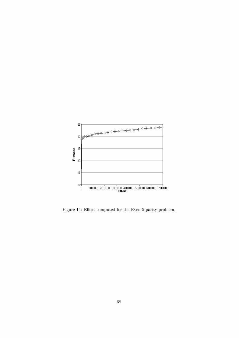
Figure 14: Effort computed for the Even-5 parity problem.

68

List of Figures

1 Pseudocode of the slice process. . . . . . . . . . . . . . . . . . . . . . . . . . . . . 12

2 Pseudocode for data movement. . . . . . . . . . . . . . . . . . . . . . . . . . . . . 16

3 Load balancing strategy: each fold is divided in four strips. . . . . . . . . . . . . 18

4 Experimental results for symbolic regression: (a) comparison between Canoni-

cal GP and CAGE, (b) convergence for different replacement policies and (c)

convergence for different population sizes. . . . . . . . . . . . . . . . . . . . . . . 58

5 Experimental results for discovery of trigonometric identities: (a) comparison be-

tween Canonical GP and CAGE, (b) convergence for different replacement policies

and (c) convergence for different population sizes. . . . . . . . . . . . . . . . . . . 59

6 Experimental results for symbolic integration: (a) comparison between Canon-

ical GP and CAGE, (b) convergence for different replacement policies and (c)

convergence for different population sizes. . . . . . . . . . . . . . . . . . . . . . . 60

7 Experimental results for Even-4 parity: (a) comparison between Canonical GP

and CAGE, (b) convergence for different replacement policies and (c) convergence

for different population sizes. . . . . . . . . . . . . . . . . . . . . . . . . . . . . . 61

8 Experimental results for Even-5 parity: (a) comparison between Canonical GP

and CAGE, (b) convergence for different replacement policies and (c) convergence

for different population sizes. . . . . . . . . . . . . . . . . . . . . . . . . . . . . . 62

9 Experimental results for Ant Santa Fe: (a) comparison between Canonical GP

and CAGE, (b) convergence for different replacement policies and (c) convergence

for different population sizes. . . . . . . . . . . . . . . . . . . . . . . . . . . . . . 63

69

10 Experimental results for Royal Tree: (a) comparison between Canonical GP and

CAGE, (b) convergence for different replacement policies and (c) convergence for

different population sizes. . . . . . . . . . . . . . . . . . . . . . . . . . . . . . . . 64

11 Snapshot of the size of the trees at the 10th (a), 20th (b), 30th (c) and 40th (d)

generation for Even-4. Different colors denote different sizes. . . . . . . . . . . . 65

12 Experimental results for cos2x: (a) CAGE and (b) Niwa and Iba. . . . . . . . . . 66

13 Experimental results for even-4 parity problem: (a) CAGE and (b) Niwa and Iba. 67

14 Effort computed for the Even-5 parity problem. . . . . . . . . . . . . . . . . . . . 68

70

List of Tables

1 CAGE Parameters . . . . . . . . . . . . . . . . . . . . . . . . . . . . . . . . . . . 26

2 Terminal symbols and functions for each problem. . . . . . . . . . . . . . . . . . 27

3 Results for Canonical GP . . . . . . . . . . . . . . . . . . . . . . . . . . . . . . . 36

4 Results of CAGE . . . . . . . . . . . . . . . . . . . . . . . . . . . . . . . . . . . . 37

5 Even-4 parity problem parameters (Cray T3E) . . . . . . . . . . . . . . . . . . . 39

6 Cray T3E execution time predictions for 100 iterations (Even-4 parity problem) . 40

7 Ant problem parameters (Cray T3E) . . . . . . . . . . . . . . . . . . . . . . . . . 42

8 Cray T3E execution time predictions for 100 iterations (Ant problem) . . . . . . 43

9 wins and losses . . . . . . . . . . . . . . . . . . . . . . . . . . . . . . . . . . . . . 48

71