Theme: National and International Governance Challenges.

Cellular automata and Genetic Algorithms based urban growth

visualization for appropriate land use policies

Uttam Kumar1 [uttam@ces.iisc.ernet.in]

Mukhopadhyay C.2 [cm@mgmt.iisc.ernet.in] &

Ramachandra T. V.3,* [cestvr@ces.iisc.ernet.in]

1 Department of Management Studies & Centre for Sustainable Technologies, Indian Institute of Science, Bangalore.

2 Department of Management Studies, Indian Institute of Science, Bangalore. 3 Centre for Ecological Sciences; Centre for Sustainable Technologies & Centre for

Infrastructure, Sustainable Transport and Urban Planning (CiSTUP), Indian Institute of Science, Bangalore.

Citation: Uttam Kumar, Chiranjit Mukhopadhyay and Ramachandra T. V., (2009), Cellular automata and Genetic Algorithms based urban growth visualization for appropriate land use policies, Proceedings of the Fourth Annual International Conference on Public Policy and Management, Centre for Public Policy, Indian Institute of Management (IIMB), Bangalore, India, 9-12 August, 2009.

Cellular automata and Genetic Algorithms based urban growth

visualization for appropriate land use policies

Abstract

Many regional environmental problems are the consequence of anthropogenic activities

involving land cover changes. Temporal land cover data with social aspects are critical in

tracing relationships of cause and effect on variables of interest with the effects of context on

behaviour or with the process of human environment interaction and are also useful for

governance of urbanising cities. Many cities are now undergoing redevelopment for economic

purposes with new roads, infrastructure improvements, etc. This phenomenona is very rapid in

India with urban population growing at around 2.3 percent per annum. This dramatic increase

in urbanisation has raised the necessity to understand the dynamics of urban growth process for

planning of natural resources. Cellular automata, an artificial intelligence technique based on

pixels, states, neighbourhood and transition rules, is being implemented to model the urban

growth process due to its ability to fit such complex spatial nature using simple and effective

rules. The possibility of using genetic algorithms for automatic calibration of the model through

proper design of their parameters, including objective function, initial population, selection,

crossover and mutation has also been explored. The techniques are tested for Bangalore city,

India by modeling the urban growth using remote sensing data of various resolutions.

Key words: land use model, urban growth, cellular automata, governance

1. Introduction

Urban growth modeling is getting more attention as an emerging research area in many

disciplines. Urbanisation is a form of metropolitan growth that is a response to often bewildering

sets of economic, social, and political forces and to the physical geography of an area. This

comes as a result of the recent dramatic increase in urban population that increases the pressure

on the infrastructure services. Many cities are now undergoing redevelopment for economic

purposes with new roads, infrastructure improvements, etc. This phenomenona is very rapid in

India with urban population growing at around 2.3 percent per annum (World Urbanization

Prospects, 2005). An increased urban population and growth in urban areas is irreversible with

population growth and migration. This dramatic increase in urbanisation has raised the necessity

to understand the dynamics of urban growth process for planning of natural resources. It also

raises the necessity to understand the dynamics of urban growth process through “growth

models” for sustainable distribution of usable resources.

Among the developed growth models, cellular automata (CA), an artificial intelligence technique

based urban growth models have better performance in simulating urban development than

conventional mathematical models (Batty and Xie, 1994). CA simplifies the simulation of

complex systems (Waldrop, 1992). Its aptness in urban modelling is due to the fact that the

process of urban spread is entirely local in nature (Clarke and Gaydos, 1998). CA is based on

pixels, states, neighbourhood and transition rules, and is being implemented to model the urban

growth process due to its ability to fit complex spatial nature using simple and effective rules.

Development of CA model involves rule definition and calibration to produce results consistent

with historical data, and future prediction with the same rules (Clarke et al., 1997). Many CA-

based urban growth models are reported in literatures including the model by White and Engelen

(1992; 1993) that involves reduction of space into square grids. They implement the defined

transition rules in recursive form to match the spatial pattern. One of the earliest and most well-

known models is CA-based “SLEUTH” model that has four major types of data: land cover,

slope, transportation, and protected lands (Clarke’s et al., 1997). This is rooted in the work of

von Neumann (1966), Hagerstrand (1967), Tobler (1979) and Wolfram (1994). A set of initial

conditions in SLEUTH is defined by ‘seed’ cells which are determined by locating and dating

the extent of various settlements identified from historical maps, atlases, and other sources.

These seed cells represent the initial distribution of urban areas. A set of complex behaviour

rules are developed that involves selecting a location randomly, investigating the spatial

properties of the neighboring cells, and urbanising the cell based on a set of probabilities.

Despite these achievements in CA urban growth modeling, the selection of CA transition rules

remains a research topic. Most of the CA models are usually designed based on individual

preference and application requirements with transition rules being defined in an ad hoc manner

(Li and Yeh, 2003). Furthermore, most of the developed CA models need intensive computation

to select the best parameter values for accurate modeling. This motivates development and

implementation of an effective CA-based urban growth model that is easy to calibrate and takes

into account the spatial and temporal dynamics of urban growth simultaneously. The objectives

of this study are:

(i) To develop and implement an effective CA-based urban growth model to simulate the

growth as a function of local neighbourhood structure of the input data.

(ii) To develop a calibration algorithm that takes into consideration spatial and temporal

dynamics of urban growth.

Spatially, the model is calibrated locally to take into account the effect of site specific features

while the temporal calibration is set up to adapt the model to the changes over growth pattern

with time. Calibration provides the optimal values for the transition rules to achieve accurate

urban growth modeling. The input to the urban growth model consists of two types of data:

(i) classified images of 1973, 1992 and 2006 where each pixel represents one of the four

land use classes – urban, vegetation, water and others.

(ii) population density maps being represented by pixels in a raster format for the year

1973 and 1992.

CA generates transition rules for each pixel based on the current state of the pixel’s category (in

terms of land use class) and population density value of that pixel together, to decide the next

state of the pixel after a time epoch, i.e. change in land use from one class to another from 1973

to 1992 and 1992 to 2006. The model is tested for Bangalore city, India by modeling the growth

using remote sensing data of various spatial, spectral and temporal resolutions. Later, towards the

end of this communication, genetic algorithm (GA) is introduced as a heuristic optimisation

technique for selecting optimal model parameters. The possibility of using GA for automatic

calibration of the model through proper design of their parameters, including objective function,

initial population, selection, crossover and mutation has been explored. Here, a set of strings are

used as initial population over which GA runs till convergence.

The paper is organized as follows: section 2 briefs the study area, followed by data preparation

details in section 3 – classification of remote sensing data of three time periods (1973, 1992 and

2006) and generation of population density maps corresponding to the year 1973 and 1992.

Section 4 introduces CA; section 5 presents the simulated results from the CA model; section 6

deals with implementation of GA to model urban growth; section 7 discusses the results of

modeling the urbanisation process and its relation to public policy followed by concluding

remarks in section 8.

2. Study Area

Bangalore city is the principal administrative, cultural, commercial, industrial, and knowledge

capital of the state of Karnataka. The administrative jurisdiction was widened in 2006 by

merging the existing area of Bangalore city spatial limits with 8 neighbouring Urban Local

Bodies (ULBs) and 111 Villages of Bangalore Urban District to form Greater Bangalore.

Bangalore has spatially grown more than ten times since 1949 from 69 square kilometers to 741

square kilometers in 2006. Now, Bangalore (figure 1) is the fifth largest metropolis in India

currently with a population of about 7 million (Ramachandra and Kumar, 2008).

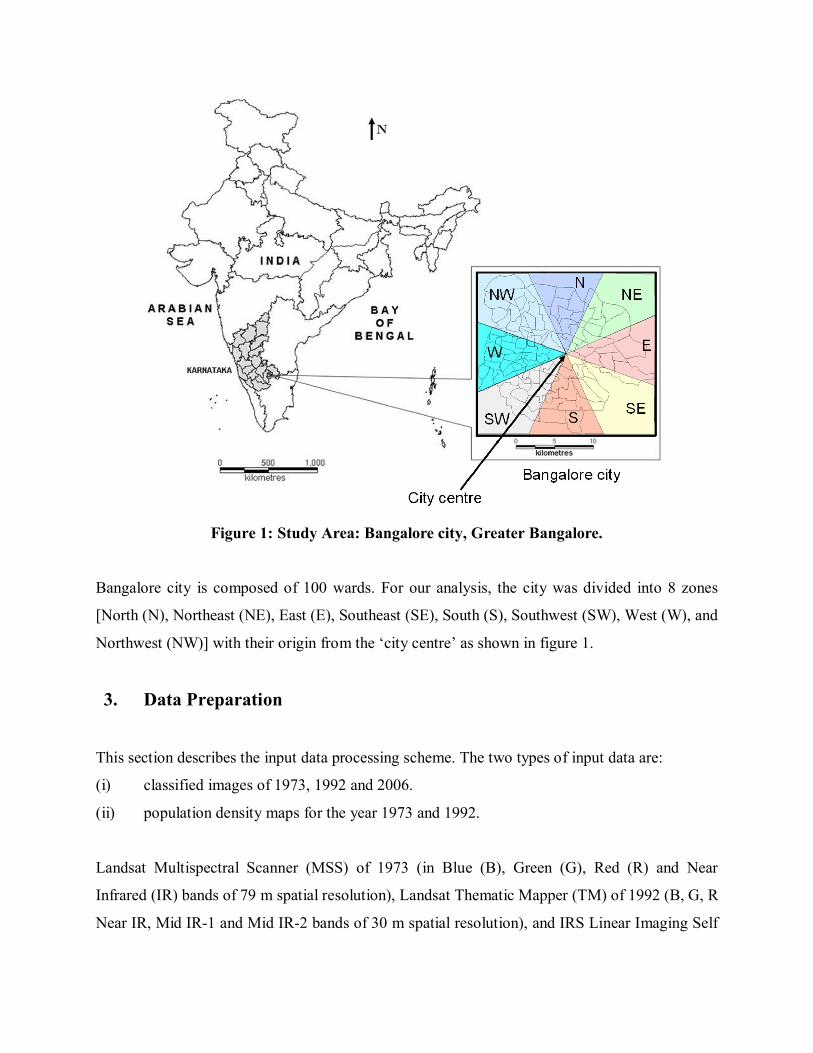
Figure 1: Study Area: Bangalore city, Greater Bangalore.

Bangalore city is composed of 100 wards. For our analysis, the city was divided into 8 zones

[North (N), Northeast (NE), East (E), Southeast (SE), South (S), Southwest (SW), West (W), and

Northwest (NW)] with their origin from the ‘city centre’ as shown in figure 1.

3. Data Preparation

This section describes the input data processing scheme. The two types of input data are:

(i) classified images of 1973, 1992 and 2006.

(ii) population density maps for the year 1973 and 1992.

Landsat Multispectral Scanner (MSS) of 1973 (in Blue (B), Green (G), Red (R) and Near

Infrared (IR) bands of 79 m spatial resolution), Landsat Thematic Mapper (TM) of 1992 (B, G, R

Near IR, Mid IR-1 and Mid IR-2 bands of 30 m spatial resolution), and IRS Linear Imaging Self

Scanner (LISS) - III of 2006 (in G, R and NIR bands of 23.5 m spatial resolution) were used for

the generation of land use maps. The data are stored in 8-bit format, i.e. each pixel can take any

value from 0 to 255 (28 = 256 values). The values of these pixels in the image are called digital

numbers which represents the reflectance represented by that pixel corresponding to the same

geographical location on the ground. The 1973 image was of size 429 rows x 445 columns, size

of 1992 image was 1130 x 1170 and the size of 2006 image was 1445 x 1496. The differences in

the size of the images are due to variations in the spatial resolution of the pixels (79 m, 30 m, and

23.5 m). These data were rectified and registered for systematic errors with the known ground

control points that were identifiable in the image as well as Survey of India (SOI) topographical

sheets of 1:50000 scale and projected to Polyconic system with Geographic Latitude-Longitude

coordinate system and Evrest56 as the datum. All data were resampled to 23.5 m spatial

resolution having 1445 rows x 1496 columns to fit each other spatially. Six classes of interest

were identified from the false colour composite images: residential areas, commercial areas,

roads, vegetation, water, and open land.

Supervised classification of the image was performed using the Maximum Likelihood classifier

(MLC). MLC has become popular and widespread in remote sensing because of its robustness

(Strahler, 1980; Conese and Maselli, 1992; Ediriwickrema and Khorram, 1997; Zheng et al.,

2005). MLC assumes that each class in each band can be described by a normal distribution

(Bayarsaikhan et al., 2009). For each land use class (residential areas, commercial areas, roads,

vegetation, water, and open land) training samples were collected representing approximately

10% of the study area. With these 10% known pixel labels from training data, the aim was to

assign labels to all the remaining pixels in the image.

If the training data (collected from the ground cover using handheld GPS - global positioning

system) pertaining to land use classes contain n samples and the samples in each land use class

are i.i.d (independent and identically distributed) random variables and further if we assume that

the spectral classes for an image is represented by ωi, i=1,…, M, where M is the total number of

classes, then probability density p(ωi|x) gives the likelihood that the pixel x belongs to class ωi

where x is a column vector of the observed digital number (gray values) of the pixels. It

describes the pixel as a point in multispectral space (d-dimensional space, where d is the number

of remote sensing spectral bands). The maximum likelihood (ML) parameters are estimated from

representative i.i.d samples. Classification is performed according to

( | ) ( | ) for all .i i jif p p j i x x x (1)

i.e., the pixel x belongs to class ωi if p(ωi|x) is the largest. The ML decision rule is based on a

normalized (Gaussian) estimate of the probability density function of each class. The

discriminant function for MLC is expressed as

lig ( ) = ( | ) ( )i ip p x x (2)

where gli(x) stands for the discriminant function for ωi, p(ωi) is the prior probability of ωi,

p(x|ωi) is the p.d.f. for pixel vector x conditioned on ωi (Zheng et al., 2005). Pixel vector x is

assigned to the class for which gli(x) is greatest. In an operational context, the logarithm form of

(2) is used, and after the constants are eliminated, the discriminant function for ωi is stated as

1liG ( ) ( ) ( ) ln | | 2 ln ( )T

i i i i iM M P x x x (3)

where i is the variance-covariance matrix of ωi, Mi is the mean vector of ωi. A pixel is

assigned to the class with the lowest liG ( )x (Zheng et al., 2005; John and Xiuping, 1999, Duda,

Hart and Stork, 2001).

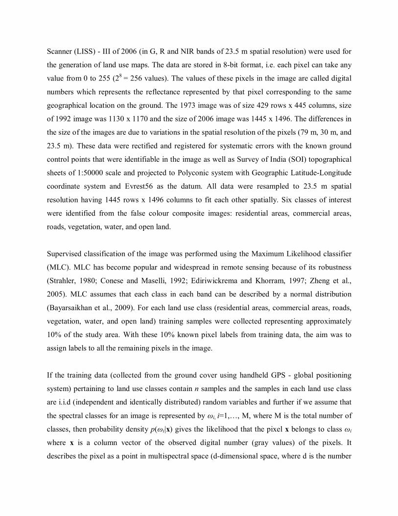
Residential, commercial and roads were grouped into a single class – ‘urban’. Final classified

images had four land use classes – builtup, vegetation, water and open land (others). The

classified images of 1973, 1992 and 2006 had overall accuracies of 72%, 75%, and 73%.

Classification was done using the open source programs (i.gensig, i.class and i.maxlik) of

Geographic Resources Analysis Support System (http://wgbis.ces.iisc.ernet.in/grass) as

displayed in figure 2. The classified images were also verified with field visits and Google Earth

image. The class statistics is given in table 1.

Table 1: Greater Bangalore land use statistics

Class Year

Urban Vegetation Water Bodies Open land

1973 Ha 5448 46639 2324 13903 % 7.97 68.27 3.40 20.35

1992 Ha 18650 31579 1790 16303 % 27.30 46.22 2.60 23.86

2006 Ha 29535 19696 1073 18017 % 43.23 28.83 1.57 26.37

Figure 2: Greater Bangalore in 1973, 1992 and 2006.

Population density is used as the second input for the CA model algorithm. Population census

maps for year 1971, 1991 and 2001 over Bangalore city were prepared from the census data. The

population densities were computed for all 100 wards by dividing their populations by the ward

areas. Figure 3 shows the ward map (left) in each direction and the density for each ward census

(right) in 1971, 1991 and 2001. To model the population, the centroid (Xc, Yc) for each ward is

calculated.

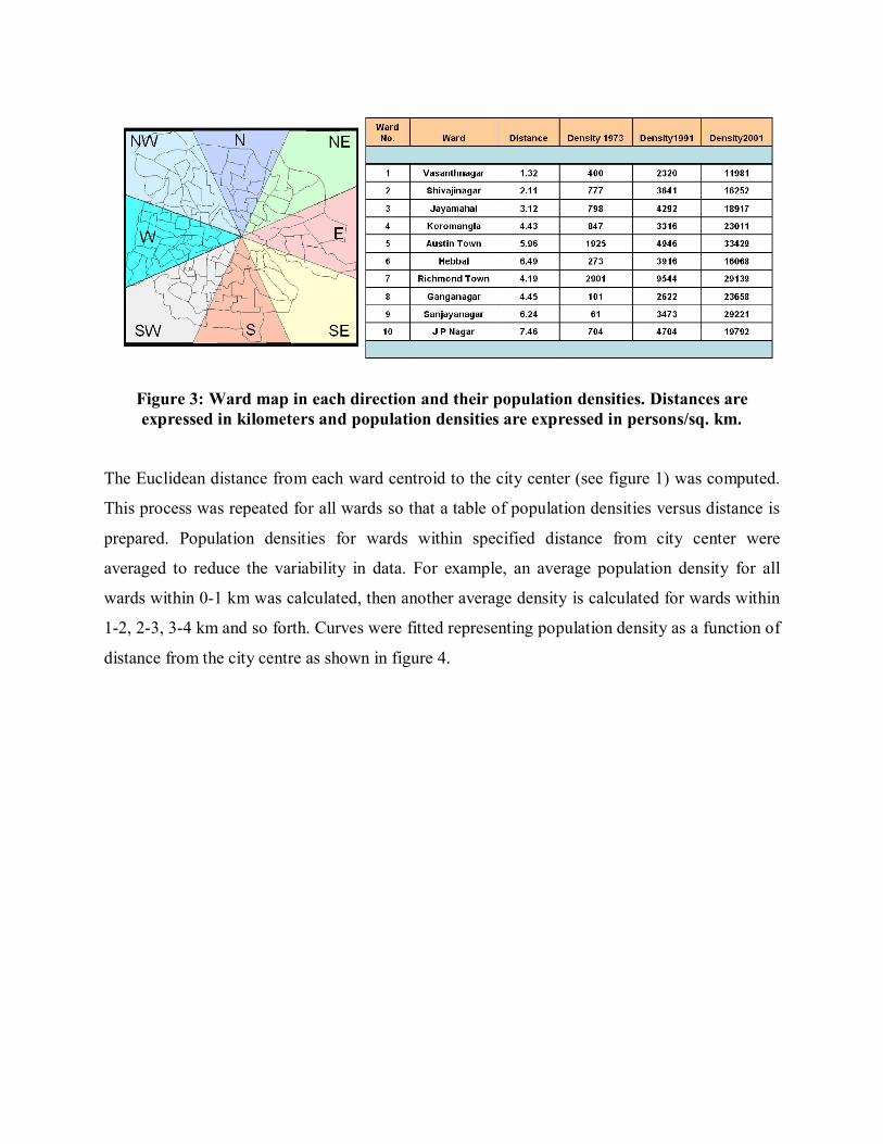
Figure 3: Ward map in each direction and their population densities. Distances are expressed in kilometers and population densities are expressed in persons/sq. km.

The Euclidean distance from each ward centroid to the city center (see figure 1) was computed.

This process was repeated for all wards so that a table of population densities versus distance is

prepared. Population densities for wards within specified distance from city center were

averaged to reduce the variability in data. For example, an average population density for all

wards within 0-1 km was calculated, then another average density is calculated for wards within

1-2, 2-3, 3-4 km and so forth. Curves were fitted representing population density as a function of

distance from the city centre as shown in figure 4.

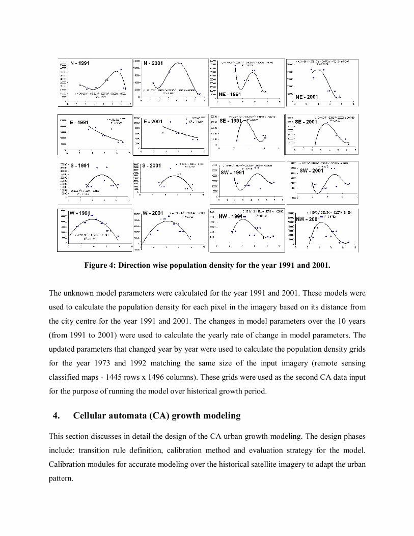
Figure 4: Direction wise population density for the year 1991 and 2001.

The unknown model parameters were calculated for the year 1991 and 2001. These models were

used to calculate the population density for each pixel in the imagery based on its distance from

the city centre for the year 1991 and 2001. The changes in model parameters over the 10 years

(from 1991 to 2001) were used to calculate the yearly rate of change in model parameters. The

updated parameters that changed year by year were used to calculate the population density grids

for the year 1973 and 1992 matching the same size of the input imagery (remote sensing

classified maps - 1445 rows x 1496 columns). These grids were used as the second CA data input

for the purpose of running the model over historical growth period.

4. Cellular automata (CA) growth modeling This section discusses in detail the design of the CA urban growth modeling. The design phases

include: transition rule definition, calibration method and evaluation strategy for the model.

Calibration modules for accurate modeling over the historical satellite imagery to adapt the urban

pattern.

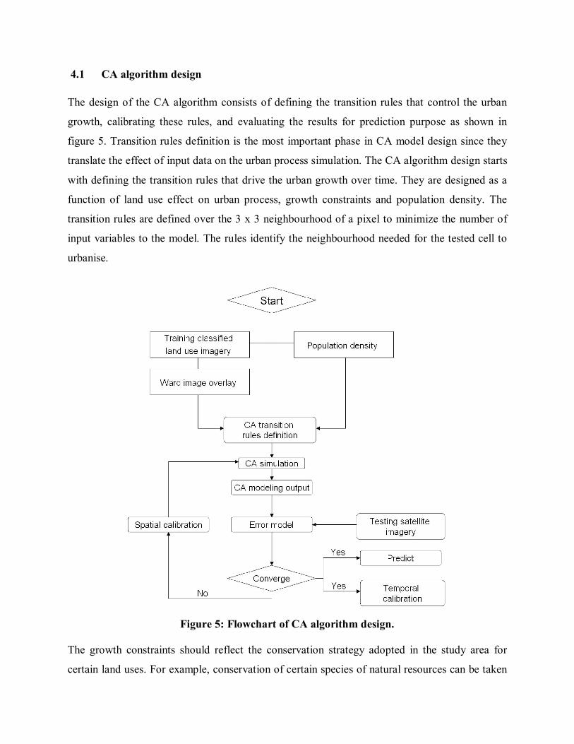
4.1 CA algorithm design The design of the CA algorithm consists of defining the transition rules that control the urban

growth, calibrating these rules, and evaluating the results for prediction purpose as shown in

figure 5. Transition rules definition is the most important phase in CA model design since they

translate the effect of input data on the urban process simulation. The CA algorithm design starts

with defining the transition rules that drive the urban growth over time. They are designed as a

function of land use effect on urban process, growth constraints and population density. The

transition rules are defined over the 3 x 3 neighbourhood of a pixel to minimize the number of

input variables to the model. The rules identify the neighbourhood needed for the tested cell to

urbanise.

Figure 5: Flowchart of CA algorithm design.

The growth constraints should reflect the conservation strategy adopted in the study area for

certain land uses. For example, conservation of certain species of natural resources can be taken

into consideration through rules definition stage. Water resources protection through

discouraging urban growth nearby these sites to preserve them over time is another example of

constrained rules design. The future state of a pixel (Equation 4) at time (t+1) from starting time

(t) depends on three factors:

Current state of the pixel

Current states of the neighbourhood pixels

Transition rules that drive the urban growth over time

1( ) ( ( ), ( ), _ )t t tS f S S transition rules ….. (Equation 4)

where

1( )tS = test pixel future state at time epoch t+1

( )tS = test pixel current state at time epoch t

( )tS = neighbourhood pixels states’ set.

4.2 CA Model calibration

Calibration aims to define the best set of CA rules based on which the model runs to match as

close as possible to the simulated results with the ground truth images. To achieve this purpose,

two calibration schemes are introduced in this algorithm: spatial and temporal calibrations. In

spatial calibration module, the CA transition rules at a given time t are modified spatially over

the 2D grid space. This is done through tuning the values of each rule set on a directional basis to

match the urban dynamics for each township with its site specific features. This allows the model

to take the variability in the spatial urban growth pattern into account for realistic modeling. If

the CA rules in a direction result in higher growth levels (overestimated), they are modified to

reduce the urban growth in that direction. For the underestimation case, the rule values of the

direction under consideration are tuned to increase the amount of urban growth to match the real

one. So, the spatial calibration aims to find the best set of rule values that fit a given direction

according to its geographical location.

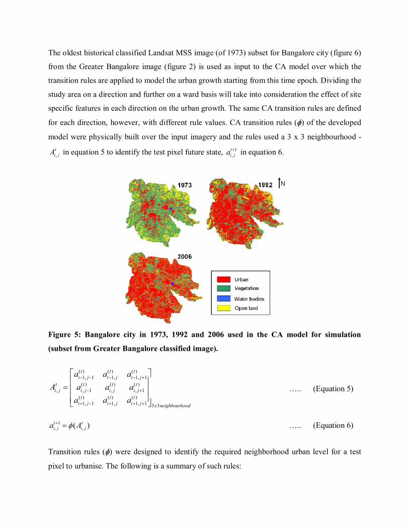
The oldest historical classified Landsat MSS image (of 1973) subset for Bangalore city (figure 6)

from the Greater Bangalore image (figure 2) is used as input to the CA model over which the

transition rules are applied to model the urban growth starting from this time epoch. Dividing the

study area on a direction and further on a ward basis will take into consideration the effect of site

specific features in each direction on the urban growth. The same CA transition rules are defined

for each direction, however, with different rule values. CA transition rules () of the developed

model were physically built over the input imagery and the rules used a 3 x 3 neighbourhood -

,ti jA in equation 5 to identify the test pixel future state, 1

,ti ja in equation 6.

Figure 5: Bangalore city in 1973, 1992 and 2006 used in the CA model for simulation

(subset from Greater Bangalore classified image).

( ) ( ) ( )

1, 1 1, 1, 1

( ) ( ) ( ), , 1 , , 1

( ) ( ) ( )1, 1 1, 1, 1 3 3

t t ti j i j i j

t t t ti j i j i j i j

t t ti j i j i j x neighbourhood

a a a

A a a a

a a a

….. (Equation 5)

1

, ,( )t ti j i ja A ….. (Equation 6)

Transition rules () were designed to identify the required neighborhood urban level for a test

pixel to urbanise. The following is a summary of such rules:

1. IF test pixel is water, road OR urban (residential or commercial) THEN no change.

2. IF test pixel is non-urban (vegetation OR open land) THEN it becomes urban if its:

Population density is equal or greater than threshold (Pi) AND neighbouring

residential pixel count is equal or greater than threshold (Ri)

where (R,C)i are integer numbers ranging from 0 to 8 (3 x 3 neighborhood) and Pi is a real

number ranging from 0 to 1 (0.1 increment; population density values were normalized from 0 to

1 for each direction in order to have effective CA rules calibration). The calibration (i.e.,

identifying best (R,P)i parameter values) of such rules was performed spatially on a ward level,

Tw to fit the local urban dynamic features and over time to consider the temporal urban changes

in each direction, Tt in (7).

Ø calibrated = f(Tw, Tt, ) ….. (Equation 7) in the calibration formula represents the criteria selected to find the best rule set for certain

ward spatial location Tw at given time epoch Tt. This criterion in our model represents the total

modeling errors/mismatch between modeled output and reality that need to be minimised or best

match. in (8) was defined as a function of fitness F in (9) and total errors ∆E in (10) valuation

measures. Fitness and total errors measure the compatibility in terms of urban count and pattern

within each township with respect to reality, respectively (Al-Kheder, et al., 2007).

( 100%)Abs F E ….. (Equation 8)

_ _

100%_ _ _

Modele urban countF

Ground truth urban count ….. (Equation 9)

_ _

100%_

Total error countE

Total count ….. (Equation 10)

Once the CA transition rules were identified and initialized for each direction, the model runs

from 1973 till 1992. The 1992 image represents the first ground truth being used for calibration.

For each ward, the modeling accuracy is calculated as a ratio between the simulated and real

urban growth data. Over/underestimation concept is introduced to represent how comparable is

the simulated result to the real one. This indicates how transition rules defined on a directional

basis succeed in modeling the real amount of urban growth given the predefined conditions.

Calibration in this work is meant to find the best set of rule values specific to each direction for

realistic urban growth modeling.

5. Results

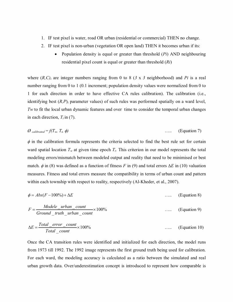
Simulation and prediction urban modeling results, as shown in table 2 and figure 6 shows a less

close match to the reality from 1973 to 1992 in terms of urban count, however, the pattern

matches in various directions to some extent.

Figure 6: Classified image of 1973, real image and simulated image of 1992. Red colour

indicates urban areas, yellow represents other classes (vegetation, water or open land) in

real and simulated images.

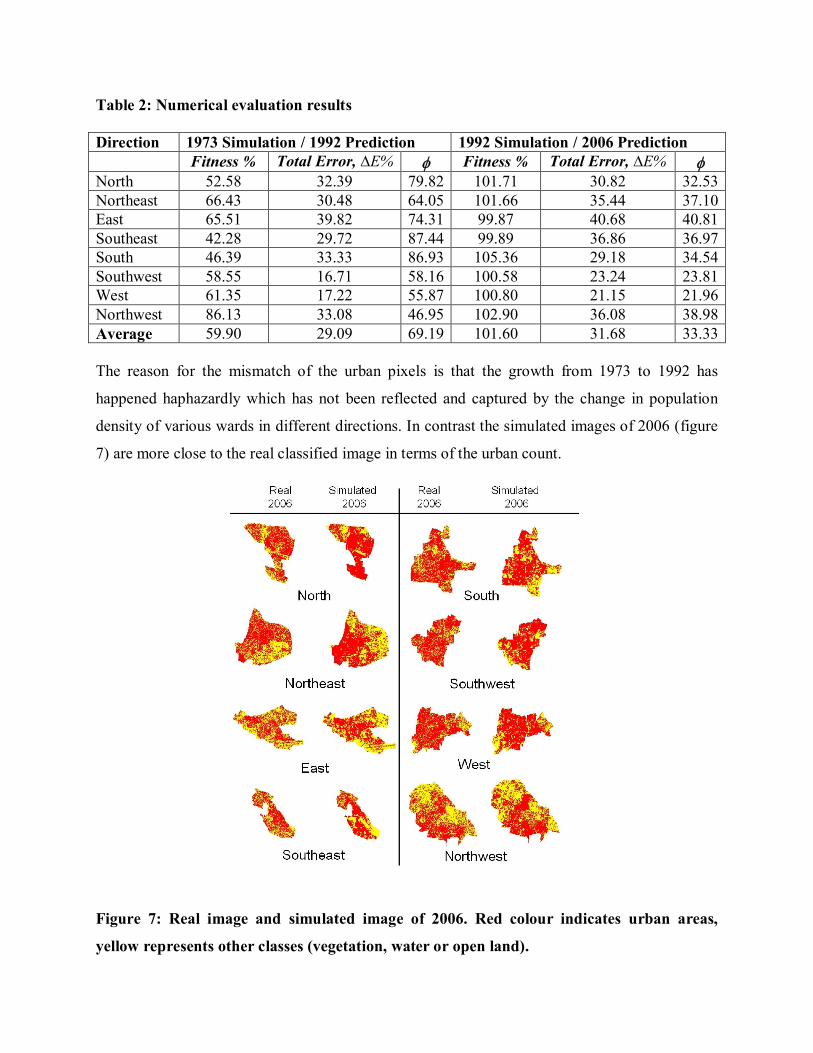
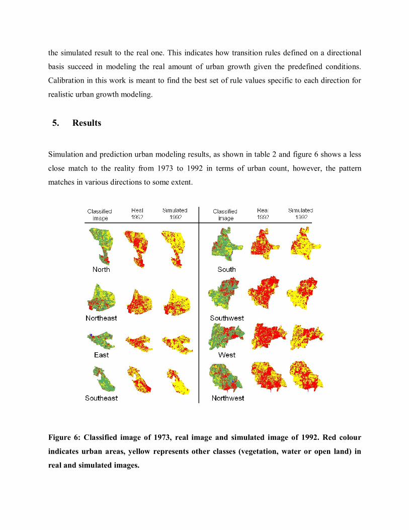
Table 2: Numerical evaluation results Direction 1973 Simulation / 1992 Prediction 1992 Simulation / 2006 Prediction Fitness % Total Error, ∆E% Fitness % Total Error, ∆E% North 52.58 32.39 79.82 101.71 30.82 32.53 Northeast 66.43 30.48 64.05 101.66 35.44 37.10 East 65.51 39.82 74.31 99.87 40.68 40.81 Southeast 42.28 29.72 87.44 99.89 36.86 36.97 South 46.39 33.33 86.93 105.36 29.18 34.54 Southwest 58.55 16.71 58.16 100.58 23.24 23.81 West 61.35 17.22 55.87 100.80 21.15 21.96 Northwest 86.13 33.08 46.95 102.90 36.08 38.98 Average 59.90 29.09 69.19 101.60 31.68 33.33 The reason for the mismatch of the urban pixels is that the growth from 1973 to 1992 has

happened haphazardly which has not been reflected and captured by the change in population

density of various wards in different directions. In contrast the simulated images of 2006 (figure

7) are more close to the real classified image in terms of the urban count.

Figure 7: Real image and simulated image of 2006. Red colour indicates urban areas,

yellow represents other classes (vegetation, water or open land).

6. Implementation of Genetic Algorithm (GA)

This section introduces briefly the on going study on using genetics algorithm (GA) to automate

the spatial and temporal rule calibration. GA as a heuristic optimisation technique can work over

the search space to find the most suitable solution. GA improves the efficiency of rule calibration

to select the best set of rule values for accurate modeling. GA was first introduced by Holland

(1975) as computer programs to mimic the evolutionary process in nature. GA manipulates a set

of feasible solutions to find an optimal solution and is able to find the global optimum solution

(S. Alkheder and J. Shan, 2006). The following steps describe the design of the proposed GA-

based transition rule calibration.

Step 1: Initial GA population generation: In this step, 30 set of rule values were randomly

generated as an initial population for each direction over which GA module would work. Each

rule value set was coded as a binary string and a string was designed as a combination of the rule

values. Two rules were identified to be optimised using GA.

Rule 1: The number of neighbourhood urbanised (residential plus commercial) pixels, in

the possible range of [0-8] integer values or in corresponding binary coding [0000 to

1000].

Rule 2: The population density threshold, continuous values represent the cut-off

population density at a pixel. This rule was scaled by multiplying its value by 10 in the

range of [0-10] possible values or in binary coding [0000 to 1010].

Step 2: Fitness function identification: Fitness function evaluates the performance of each

string. The prediction accuracy was used as the fitness function.

Step 3: GA selection operation: Rank selection procedure was used here. All the strings were

ordered based on their fitness values in descending order and the string with highest fitness value

was given rank 30 then the second one 29 till lowest fitness value with rank 1. Rank was divided

by the summation of all the ranks and the probability of selection for each string in next

generation was identified.

Step 4: GA crossover and mutation parameters design: The crossover

probability was selected to be 80%, 24 strings were selected for crossover, while the other 6 (the

best 6 in terms of fitness values) were copied directly to the new generation (this process is

known in GA as Elitism). Elitism can rapidly increase the performance of GA, because it

prevents a loss of the best solution. A mutation rate of 1% was used. Once the crossover and

mutation was done, the new generation of 30 strings was produced and the loop continued. This

continued until the convergence criterion was met. The final output was the optimized CA rule

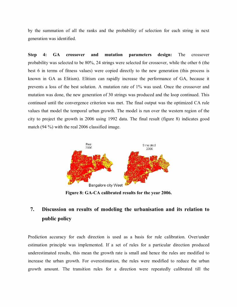
values that model the temporal urban growth. The model is run over the western region of the

city to project the growth in 2006 using 1992 data. The final result (figure 8) indicates good

match (94 %) with the real 2006 classified image.

Figure 8: GA-CA calibrated results for the year 2006.

7. Discussion on results of modeling the urbanisation and its relation to

public policy

Prediction accuracy for each direction is used as a basis for rule calibration. Over/under

estimation principle was implemented. If a set of rules for a particular direction produced

underestimated results, this mean the growth rate is small and hence the rules are modified to

increase the urban growth. For overestimation, the rules were modified to reduce the urban

growth amount. The transition rules for a direction were repeatedly calibrated till the

convergence criterion is met. The classified image provides the reference for calibration process.

In table 2, the Fitness %, Total Error (∆E %) and values for the year 1992 indicates a poor

match of the simulated image with the real image (classified image), which is an indication of

underestimation of urban pixels in various directions. However, the results for the 2006

simulated image (table 2), indicates very good spatial prediction accuracy. The spatial variability

between the various directions as compared to the real image is small. This indicates the effect of

spatial calibration in matching each direction with its realistic urban growth pattern through

calibrating its rules. It also helped in capturing finer details in the modeling process while

calibrating the model over smaller spatial units to reduce modeling uncertainty. Visually,

calibration on a directional basis succeeds in preserving the urban pattern over space and over

time. Rule values’ results at the end of the calibration process indicate some similarity between

growth in various directions such as the east, west and the northwest. These wards have almost

the same growth rate and pattern because of similar infrastructure, facilities, and more open area

for outer growth and urban sprawl. Most of these similar wards have ring roads or highways

passing through them that allow linear urban growth happening along.

The average fitness value for the 1992 image was ~ 60% and the total error was 29.09 with an

approximate match of 71%. It is to be noted that for a highly accurate prediction, the total

modeled urban count and ground truth urban count will be equal and therefore the fitness value

(F) will be 1 or 100%. The total errors ∆E is the error of omission and commission. More the

value of ∆E, more is the percentage of error count. There seems some mismatch between the

urban pixels in 1992 that is without any visible pattern and therefore could not be assessed and

captured by the change in population density contours and curve fits in various wards and

different directions. Simulation and prediction urban modeling results, as shown in table 2 for the

year 2006, show that the fitness results for prediction was close in terms of urban count (values

close to 100%) between the modeled and real data with average fitness of 101.60 (little

overestimate) and the average total error of 31.68% was achieved. This indicates an approximate

match level of 69% on a pixel by pixel basis between modeling and reality. Therefore, higher the

value of in equation 8, higher is the modeling error. For the 2006 simulated image, the average

is 33.33 showing a more realistic result as compared to the actual urban growth pattern. This is

a high accuracy level compared to the results shown in literature for the urban land spatial fit

area that was only 28.15 to 44.6% (Yang and Lo, 2003). The close urban pattern match is also

clear in figure 6 where the simulated images have urban distribution similar to those shown in

their corresponding real images.

The simulation results of urban growth should be accurate and should represent the actual local

site specific patterns close to reality since urbanisation process is directly linked to society,

infrastructure, level of services, etc. At this point of time, it would be appropriate to link people-

and-pixels in remotely sensed images. One rationale for doing so is that, it might result in better

social science research in several ways – such as measuring the context of social phenomena and

their effects while providing additional measures, making connections across levels of analysis,

providing time-series data on socially relevant phenomena. On the other hand, social science has

also to play a major role for remote sensing. Social science makes several kinds of scientific

contributions to remote sensing such as validation and interpretation of remote observations, data

confidentially and public use, etc. Together remote sensing mapping technology and social

science can improve understanding of human-environment interactions to a great extent. They

help in interpreting, modeling, predicting the dynamics of natural resources, and in

understanding the human consequences of climate flux, etc.

The change in land use such as agricultural fields, buildings, roads are often considered human

artifacts and gets less importance and are therefore less interesting than the abstract variables that

explain their appearance and transformations. Changing land use are regarded as manifestations

of more important variables, such as government policies, land-tenure rules, distribution of

wealth and power, market mechanisms, and social customs, none of which are directly reflected

in the bands of the electromagnetic spectrum. The social utility argument posits that the

interpretation of classified images obtained from remote sensing imageries becomes even more

valuable to the extent that social scientist find useful, and that efforts should be made to identify

and overcome the existing barriers to making this happen. From the perspective of social science,

one important reason for using remotely sensed data is to gather information on the context that

shapes social phenomena. The role of context has been central to the theories and empirical work

of numerous statisticians, sociologists, economists, and anthropologists. In this context, remote

sensing technology offers an additional source of contextual data for multilevel analyses.

Another consideration involves the growing interdisciplinary community ranging from

sustainable development, pollution prevention, global environmental change, to related issues of

human-environment interaction who need to compare data on social and environmental

phenomena at the same spatial and temporal scales (Liverman et al., 1998). Therefore, the

consideration of spatial and temporal resolutions is very important.

Another critical issue in linking people with pixels and image is the decision on where to

gereference individuals or other social units. The approach adopted in this work aggregates

social data to larger geographical units; assigning individuals to larger areas in which their

environmental effects are more likely to be confined. It is necessary at this point of time, to

socialise the pixel and pixelise the social in land use and land cover change. Mining the pixel

involves seeking social meaning in imaginary – information and indicators relevant to such

concerns as economic well-being or criticality, perhaps signaling the underlying processes that

give rise to land use and land cover change. This meaning is often hidden deep within the

analysis of the imagery and this depth may impede such investigation. A paucity of spatially

explicit data has constrained spatial modeling of human behavior and social structures, especially

beyond the field of geography and has fostered modeling approaches that abstract the essential

spatial nature of the problem. As a result, either aggregate relationships are specified, or the

spatial components in a model are reduced to unidimensional variables, such as the distance

between economic activities in location model, the wage differential in a migration model, or the

cost of access in a transportation model. The increased availability of spatially explicit data, both

remotely sensed and other data, and GIS (Geographic Information System) has begun to change

the situation. Advances are being made to link on-the-ground human actions and consequences

to imagery (pixels) through models, or modeling to the pixel, as in modeling the determinants of

the decision of individual land managers on the basis of utility maximisation, satisficing, or other

theories of human behavior. The use of pixels may extend to explain the dynamics of many

indicators such as energy demand and conservation, environmental area assessment, disaster

energy response, forecasting urban expansion that can be visualized as concentric rings, sectors

or multiple nuclei.

The future interaction between societal studies and remote sensing depends on what kind of

features can be detected and how often data can be obtained. Remote sensing technology may be

used not only for monitoring change, but also for conducting surveillance. For example to count

houses, to count the number of stories in each house, and detect changes in building structure.

This may provide ability to check on building regulations and thus develop some new surrogates

for social economic conditions. The key question is whether this type of information can be used

to create more efficient urban environments and provide a more equitable distribution of

resources and services?

8. Conclusion

This work explores the potential of implementing the cellular automata to model the historical

urban growth over Bangalore city. The main goal is to design the model as a function of local

neighbourhood structure to minimise the input data to the model. Satellite imagery represents the

medium over which the model works. One special issue the model takes into account is the

calibration process. Two modules were used namely, spatial and temporal calibration. Spatial

calibration fits the model on a directional basis to its site specific feature while the temporal

calibration adapts it to the urban growth dynamic change over time. This is a noticeable effect on

producing a good spatial match between the real and simulated image data. On the other hand,

GA is introduced to enhance the CA calibration process. GA makes the calibration process more

efficient through manipulating a set of feasible solutions in the search space to find an optimal

solution. This will reduce the search space for the optimal rules’ values on a directional basis.

The above techniques are robust in predicting urban growth and visualizing them through pixels

in images. Relating pixels in remote sensing data and people in society is important for studies

on sustainable development, pollution prevention, global environmental change, and issues of

human-environment interaction at different spatial and temporal scales.

9. References Alkheder, S, Shan, J., 2006, ‘Change detection - cellular automata method for urban growth

modeling’, International Society of Photogrammetry and Remote Sensing Mid-term Symposium,

WG VII/5, Netherlands, May 2006.

AlKheder, S., Wang, J., and Shan, J., 2007, ‘Cellular automata urban growth model calibration

with genetic algorithms’, Urban Remote Sensing Joint Event.

Batty, M., and Xie, Y., 1994, ‘From cells to cities’, Environment and Planning, B21, pp. 531-

548.

Bayarsaikhan, U., Boldgiv, B., Kim, K-R., Park, K-A., Lee, D., 2009, Change detection and

classification of land cover at Hustai National Park in Mongolia. International Journal of Applied

Earth Observation and Geoinformation, 11, 273-280.

Conese, C., Maselli, F., 1992, Use of error matrices to improve area estimates with maximum

likelihood classification procedures. Remote Sensing of Environment, 40, 113-124.

Clarke, K. C., Hoppen, S., and Gaydos, L., 1997, ‘A selfmodifying cellular automaton model of

historical urbanization in the San Francisco Bay area’, Environment and planning, 24, pp. 247-

261.

Clarke, K. C., and Gaydos, L. J., 1998, ‘Loose-coupling a cellular automaton model and GIS:

long-term urban growth prediction for San Francisco and Washington/Baltimore’, International

Journal of Geographical Information Sciences, 12, pp. 699-714.

Duda, R. O., Hart, P. E., and Stork, D, G., 2000, Pattern classification, New York, A Wiley-

Interscience Publication, Second Edition, ISBN 9814-12-602-0.

Ediriwickrema, L., Khorram, S., 1997, Hierarchical maximum-likelihood classification for

improved accuracies. Geoscience and Remote Sensing, IEEE Transactions, 35, 810-816.

Hagerstrand, T., 1967, ‘Innovation Diffusion as a Spatial Process’ University of Chicago Press,

Chicago, IL.

Holland, J. H., 1975, ‘Adaptation in Natural and Artificial Systems’, Univ. of Michigan Press,

Ann Arbor, MI.

John, A. R., Xiuping, J., 1999. Remote Sensing Digital image Analysis: An Introduction.

Springer-Verlag Inc., New York.

Li, X., and Yeh, A. G. O., 2003, ‘Error propagation and model uncertainties of cellular automata

in urban simulation with GIS’, In:7th International Conference on GeoComputation, 8- 10,

September 2003, University of Southampton, Southampton, UK (GeoComputation CD-ROM).

Liverman, D., Moran, E. F., Rindfuss, R. R., and Stern, P. C., 1998, People and pixels - Linking

Remote Sensing and Social Science, Washington, D. C., National Academy Press.

Ramachandra, T.V., and Kumar, U., 2008, ‘Wetlands of Greater Bangalore, India: Automatic

Delineation through Pattern Classifiers’, Electronic Green Journal, Vol. 26, Spring 2008 ISSN:

1076-7975.

Strahler, A. H., 1980. The use of prior probabilities in maximum likelihood classification of

remotely sensed data. Remote Sensing of Environment, 10, 135-163.

Tobler, W., 1979, ‘Cellular geography, in Philosophy’, In: Geography Eds S Gale, G Olsson (D

Reidel, Dordrecht), pp. 379-386.

von Neumann, J., 1966, ‘Theory of Self-Reproducing Automata’, University of Illinois Press,

Illinois. Edited and completed by A. W. Burks.

White, R. and Engelen, G. 1992. "Cellular Dynamics and GIS: Modeling Spatial Complexity",

position paper presented at the NCGIA Specialist Meeting on GIS and Spatial Analysis.

White, R. and Engelen, G. 1993. "Cellular Automata and Fractal Urban Form: A Cellular

Modeling Approach to the Evolution of Urban Land Use Patterns", Environment and Planning

A, 25, 1175-1199.

Wolfram, S., 1994, ‘Cellular automata’, In: Cellular Automata and Complexity: Collected

Papers, Addison Wesley, Steven Wolfram, Reading, MA.

World Urbanization Prospects, 2005, Revision, Population Division, Department of Economic

and Social Affaris, UN.

Yang, X, and Lo, C. P., 2003, ‘Modelling urban growth and landscape changes in the Atlanta

metropolitan area’, International Journal of Geographical Information Science, Vol. 17, pp.

463–488.

Zheng, M., Cai, Q., Wang, Z., 2005. In: Effect of prior probabilities on maximum likelihood

classifier. Geoscience and Remote Sensing Symposium, 2005, IGARS’05, Proceedings 2005

IEEE International, 6, pp. 3753-3756.

Uttam Kumar is a PhD student at the Department of Management Studies and Centre for Sustainable Technologies, Indian Institute of Science, Bangalore. His areas of research are developing algorithms for multi-satellite sensor spatial temporal data analysis. His research interests are Pattern recognition, Remote sensing, Data mining and Image processing.

Chiranjit Mukhopadhyay earned a Ph.D. in Statistics from University of Missouri, Columbia in 1992,

after obtaining M-Stat and B-Stat from Indian Statistical Institute, Kolkata. Currently he is Associate

Professor of Statistics in the Department of Management Studies, Indian Institute of Science, Bangalore.

He has served in the faculty of several Universities around the globe like The Ohio State University, Case

Western Reserve University, Bilkent University etc. His current research interests include Bayesian

Statistics, Reliability Theory, Statistical Quality Control, Empirical Finance and Financial Econometrics.

Ramachandra T. V. obtained his Ph.D. from Indian Institute of Science (IISc), Bangalore. Currently he is

a faculty at the Centre for Ecological Sciences (CES), Centre for Sustainable Technologies (CST) and

Centre for Infrstructure, Sustainable Transport and Urban Planning (CiSTUP) at IISc, Bangalore. His area

of research includes remote sensing, digital image processing, urban sprawl: pattern recognition,

modelling, energy systems, renewable systems, energy planning, energy conservation, environmental

engineering education, etc. He has published 108 research papers in national and international journals,

and has more than 75 papers in conferences. He has written 14 books on related topics. He is member of

many national and internationally recognized professional bodies and is also the Convenor, Energy

Information System (ENVIS) at IISc. He is a Member of Karnataka State level Environment Expert

Appraisal Committee (2007-2010), appointed by the Ministry of Environment and Forests, Government

of India and a member of Western Ghats task force appointed by the Government of Karnataka. He is a

recipient of 2007 Satish Dhawan Young Engineer Award, 2007 of Karnataka State Government.