A Robust Design Space Modeling - cs.nju.edu.cn

A

Robust Design Space Modeling

Qi Guo, Carnegie Mellon UniversityTianshi Chen, Institute of Computing Technology, Chinese Academy of SciencesZhi-Hua Zhou, Nanjing UniversityOlivier Temam, INRIALing Li, Institute of Automation, Chinese Academy of SciencesDepei Qian, Beihang UniversityYunji Chen, Institute of Computing Technology, Chinese Academy of Sciences

Architectural design spaces of microprocessors are often exponentially large with respect to the pendingprocessor parameters. To avoid simulating all configurations in the design space, machine learning and sta-tistical techniques have been utilized to build regression models for characterizing the relationship betweenarchitectural configurations and responses (e.g., performance or power consumption). However, it is shownin this paper that the accuracy variability of many learning techniques over different design spaces andbenchmarks can be significant enough to mislead the decision-making. This clearly indicates a high risk ofapplying techniques which work well on previous modeling tasks (each involves a design space, benchmark,and design objective) to a new task, due to which the powerful tools might be impractical.

Inspired by ensemble learning in the machine learning domain, we propose a robust framework calledELSE to reduce the accuracy variability of design space modeling. Rather than employing a single learningtechnique as previous investigations, ELSE employs distinct learning techniques to build multiple base re-gression models for each modeling task. This is not a trivial combination of different techniques (e.g., alwaystrusting the regression model with the smallest error). Instead, ELSE carefully maintains the diversity ofbase regression models, and constructs a meta-model from the base models, which can provide accuratepredictions even when the base models are far from accurate. Consequently, we are able to reduce the num-ber of cases in which the final prediction errors are unacceptably large. Experimental results validate therobustness of ELSE: compared with the widely used Artificial Neural Network over 52 distinct modelingtasks, ELSE reduces the accuracy variability by about 62%. Moreover, ELSE reduces the average predictionerror by 27% and 85% for the investigated MIPS and POWER design spaces, respectively.

Categories and Subject Descriptors: C.1.0 [Processor Architectures]: General; B.2.2 [Arithmetic andLogic Structures]: Performance Analysis and Design Aids—Simulation; I.2.6 [Artificial Intelligence]:Learning

General Terms: Algorithms, Design, Experimentation

This work is partially supported by the NSF of China (under Grants 61100163, 61133004, 61222204,61221062, 61333014, 61321491, 61303158), the 863 Program of China (under Grants 2012AA012202,2012AA010902), the Strategic Priority Research Program of the CAS (under Grant XDA06010403), the In-ternatioanal Collaboration Key Program of the CAS (under Grant 171111KYSB20130002), the 10000 talentprogram, and the DARPA PERFECT program.Authors’ addresses: Qi Guo is with Department of Electrical and Computer Engineering, Carnegie MellonUniversity, Pittsburgh, PA 15213, USA. Tianshi Chen and Yunji Chen (corresponding author: [email protected])are with State Key Laboratory of Computer Architecture, Institute of Computing Technology, ChineseAcademy of Sciences, Beijing 100190, China; Zhi-Hua Zhou is with National Key Laboratory for Novel Soft-ware Technology, Nanjing University, Nanjing 210023, China; Olivier Temam is with INRIA, France; LingLi is with Institute of Automation, Chinese Academy of Sciences, Beijing 100190, China; Depei Qian is withBeihang University, Beijing 100191, China.Permission to make digital or hard copies of part or all of this work for personal or classroom use is grantedwithout fee provided that copies are not made or distributed for profit or commercial advantage and thatcopies show this notice on the first page or initial screen of a display along with the full citation. Copyrightsfor components of this work owned by others than ACM must be honored. Abstracting with credit is per-mitted. To copy otherwise, to republish, to post on servers, to redistribute to lists, or to use any componentof this work in other works requires prior specific permission and/or a fee. Permissions may be requestedfrom Publications Dept., ACM, Inc., 2 Penn Plaza, Suite 701, New York, NY 10121-0701 USA, fax +1 (212)869-0481, or [email protected]© YYYY ACM 1084-4309/YYYY/01-ARTA $10.00

DOI 10.1145/0000000.0000000 http://doi.acm.org/10.1145/0000000.0000000

ACM Transactions on Design Automation of Electronic Systems, Vol. V, No. N, Article A, Pub. date: January YYYY.

A:2 Q. Guo et al.

Additional Key Words and Phrases: architectural simulation, design space modeling, ensemble learning

1. INTRODUCTIONA critical issue when designing a modern microprocessor is to explore the design spaceof architectural configurations, where each configuration is a combination of multi-ple architectural parameters. Design space exploration (DSE) is well known to betime-consuming, not only because evaluating each architectural configuration with thecycle-by-cycle simulation is quite slow, but also because the number of configurationsin a design space is exponentially large [Yi et al. 2006]. To effectively accelerate designspace exploration, machine learning techniques have been applied to build regressionmodels for the design space. At the cost of simulating only a small fraction of archi-tectural configurations, the regression model is able to learn the relationship betweenconfigurations and the corresponding responses (e.g., performance or energy). Relyingon the regression model, the responses of the rest architectural configurations can beattained without cycle-accurate simulations. Besides, in addition to efficiently conduct-ing DSE, regression model can also be used to conduct detailed performance analysisto identify performance issues [ElMoustapha Ould-Ahmed-Vall and Doshi 2007] orsystem optimization [Lee and Brooks 2010].

Traditionally, when recommending a technique of Empirical Design Space Modeling(EDSM), the effectiveness was often validated on a specific design space and only afew benchmarks, and there is often an assumption that a technique works well on onedesign space can universally work well on other design spaces. While acknowledgingthe effectiveness of these techniques under specific modeling tasks, we claim that thisassumption, in fact, violates the well-known No-Free-Lunch theorem [Wolpert 1997;Wolpert and Macready 1997] in the machine learning domain, which asserts that nolearning technique can universally outperform another learning technique (e.g., a to-tally random learning algorithm) under all possible modeling tasks. In the context ofEDSM, this implies that a learning technique that has been validated to perform gen-erally well under specific modeling tasks might perform badly if the design space, thedesign objective and the application have changed. As illustrated in Figure 1, the pre-diction error of Artificial Neural Network (ANN) (the most commonly used learningtechnique for EDSM [Ipek et al. 2006; Khan et al. 2007; Dubach et al. 2007; Cho et al.2007]) varies significantly over different modeling tasks where the design objectivesand benchmarks with respect to a superscalar design space are different.

The accuracy variability of a learning technique for EDSM has been so common andsignificant that when facing different modeling tasks of EDSM, sticking to a singletechnique would be rather risky. For example, in Figure 1 the third quartile percent-age error w.r.t the ANN technique can be about 8% when estimating the power forbenchmark equake, which indicates that architects may suffer from a prediction er-ror of 8% for about 25% of all design configurations. However, when facing anothermodeling task for the MIPS architecture, the third quartile prediction error couldonly be 0.55%. Furthermore, the maximal prediction errors of 10 out of 16 model-ing tasks in this design space even exceed 50% of the actual responses obtained bysimulations, and the maximal one could be more than 80% for modeling task equake-power. Due to the considerable accuracy variability, traditional learning techniquesmay mislead the decision-making by recommending an inappropriate architecturalconfiguration, especially when designing application-specific processors to meet spe-cific performance/energy requirements [Hardavellas et al. 2011].

The risk of making incorrect decisions calls for robust EDSM whose prediction overdifferent modeling tasks (e.g., different architectural design spaces, different designobjectives or different benchmarks) is more stable and accurate. In this paper, in-spired by a machine learning methodology called ensemble learning [Zhou 2012; Diet-


Robust Design Space Modeling A:3

0

10

20

30

40

50

60

70

80

90

Perc

enta

ge E

rror (

%)

Median 3rd Quartile Max

Fig. 1. The median, third quartile and maximal prediction error (in percentage) of ANN for a superscalardesign space, where 16 different modeling tasks are considered. Although ANN can achieve good predic-tion accuracy on some modeling tasks (e.g., modeling the performance of benchmark gzip on this designspace), it does not universally perform well on all 16 modeling tasks. For instance, under the modeling taskequake-power, the maximal error is 82.15%, which is significant enough to mislead the decision-making. Theevaluated design space is a POWER architecture, and it contains nearly 1 billion design options. The maindesign parameters of ANN are set as follows: each ANN contains one 16-unit hidden layer with a learningrate of 0.001, and the momentum value is 0.5. Besides, 10-fold cross-validation is utilized to obtain the aboveresults. Details of the experimental setups will be elaborated in later sections.

terich 1998] we propose a variability-reduction approach called ELSE (i.e., EnsembleLearning for design Space Exploration) to address the above issue. Briefly speaking,for each modeling task of EDSM, ELSE builds several distinct base regression models,and uses the base models to construct a meta-model which is responsible for provid-ing the final output of each prediction. ELSE is not a trivial combination of differenttechniques (e.g., always trusting the regression model with the smallest error). The basemodels are built via using different data samples, different learning techniques or thesame technique with distinct learning parameters. During this process, in addition tobuilding base models, the diversity of different base models is carefully maintained.Consequently, the overall meta-model constructed by ensemble learning can inheritthe advantages of each base model while compensating the defects of single base mod-els. Thus, it can effectively reduce the number of cases in which the final predictionerrors are unacceptably large, even if the base models are far from accurate.1 By per-forming more stably and accurately over different modeling tasks, ensemble learningenables robust design space modeling. According to our empirical study on 52 differ-ent modeling tasks involving both MIPS and POWER architecture, ELSE can reducethe accuracy variability of the widely used Artificial Neural Network (ANN) by about62% with respect to the max prediction error. Meanwhile, ELSE reduces the averageprediction error on MIPS and POWER modeling tasks by 27% and 85% respectively,compared with the average of the best accuracies obtained by three traditional learn-ing techniques.

The contributions of this paper are briefly summarized as follows. First, it is the firsttime the accuracy variability in architectural EDSM is systematically revealed and

1It is noteworthy that ensemble learning has sound theoretical foundation [Schapire 1990; Friedman et al.2000; Kuncheva 2002]; in particular, it is well-known in the machine learning community that, ensemblemethods are the most powerful technique, both theoretically and empirically, for the reduction of accuracyvariability [Opitz and Maclin 1999; Buja and Stuetzle 2000].


A:4 Q. Guo et al.

investigated over a large number of different modeling tasks. Second, a variability-reduction approach called ELSE is proposed to offer robust yet effective architecturalEDSM. ELSE is a framework of robust EDSM that does not rely on any specific learn-ing techniques, thus can seamlessly assist various regression techniques to performrobustly under distinct modeling tasks of EDSM. Third, the advantages of ELSE havebeen empirically validated over distinct design spaces and benchmarks.

The rest of the paper is organized as follows: Section 2 introduces some relatedwork about existing learning techniques for DSE. Section 3 introduces the detailedexperimental methodology of our empirical study. Section 4 studies the prediction ac-curacies of traditional learning techniques on both MIPS and POWER design spaces.Section 5 presents the framework of ELSE. Section 6 compares ELSE with traditionaltechniques. Section 7 concludes the whole paper.

2. RELATED WORKLearning/regression techniques are a type of emerging techniques for EDSM, whichhave been continually inspired by various machine learning and numerical methods.Ipek et al. [Ipek et al. 2006] utilized ANN to capture the sophisticated relationshipbetween design parameters and the performance. Almost in the same time, Lee andBrooks [Lee and Brooks 2006] used spline-based regression models to predict IPC andpower consumption for microarchitectural design. As stated by Lee and Brooks [Leeand Brooks 2010], spline-based regression models can achieve comparable accuracieswith ANN. However, it requires more human interventions and domain knowledgethan ANN, though spline-base models are much more computationally efficient thanANN [Lee and Brooks 2010]. Another important observation described in [Lee andBrooks 2006] is that no spline function can be universally promising for various mod-eling tasks [Lee and Brooks 2006], which serves as another crucial evidence to theaccuracy variability of regression models. Joshep et al. [Joseph et al. 2006] proposedto use Radius Basis Function (RBF) networks to construct a nonlinear model for per-formance prediction. To reveal the program runtime characteristics on different ar-chitectures, Cho et al. [Cho et al. 2007] utilized a novel wavelet model to predict theworkload dynamics, and the model can be utilized to capture the complex workload dy-namics across different architectures. To reduce the simulation costs for cross-programEDSM, Khan et al. [Khan et al. 2007] and Dubach et al. [Dubach et al. 2007] indepen-dently proposed to utilize signature, which is a small set of responses that are attainedvia simulating representative architectures, when building cross-program ANN-basedregression models. The experiments conducted by Dubach et al. on a unicore designspace showed that the percentage errors on energy-delay range from about 5% to 50%over different benchmarks, where the signature-based regression clearly exhibited theaccuracy variability. Lee et al. [Lee et al. 2008] proposed composable performance re-gression (CPR) model for multiprocessors. Azizi et al. [Azizi et al. 2010] investigated anarchitecture-circuit co-design space to meet energy and performance requirements. Tofacilitate marginal cost analysis, they utilized polynomial functions as the regressionmodels to predict the performance. Empirical comparisons were conducted to showthat their models are comparable with cubic spline function regarding the predictionaccuracy. In addition to such learning/regression techniques used for DSE, there arealso studies which use analytic models to cope with DSE. Palermo et al. proposedto use Response Surface Modeling (RSM) techniques to refine the design space ex-ploration and identify feasible configurations under design constraints (such as area,energy, and throughput) [Palermo et al. 2009]. Mariani et al. also leveraged RSM inthe design-time architectural exploration [Mariani et al. 2013]. Paone et al. utilizedan ANN-based ensemble learning technique to improve the simulation speed and ac-



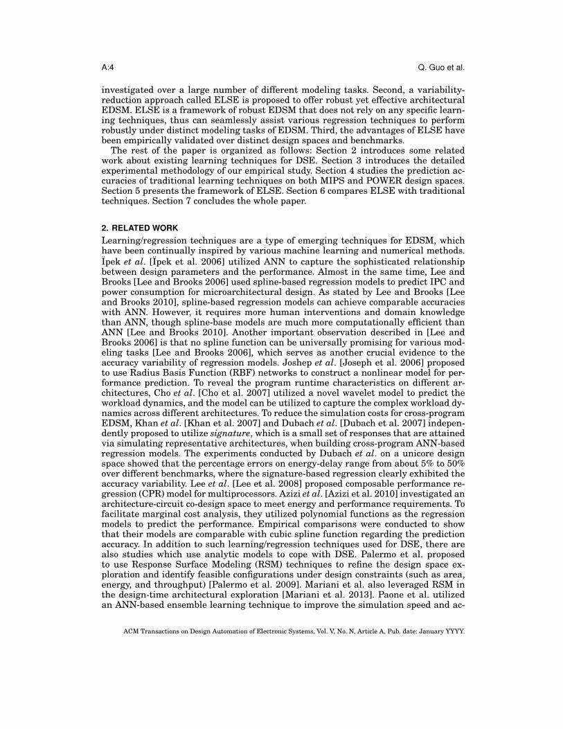
Table I. MIPS Architectural Design Space

Abbr. Variable Parameters Values NumberWIDTH Fetch/Issue/Commit Width 4,8 2

ROB ROB Size 64-160 with a step of 8 13IQ Instruction Queue Size 16-80 with a step of 8 9

LSQ Load/Store Queue Size 16-80 with a step of 8 9RF Register File Size 64-160 with a step of 8 13

L1IC L1 ICache 16,32,64,128KB 4L1DC L1 DCache 16,32,64,128KB 4L2UC L2 UCache 256KB-4MB 5BRAN Branches Allowed 8,16,24,32 4PRED Branch Predictor 1,2,4,8,16,32K 6BTB Branch Target Buffer 1,2,4K 3RAS RAS Size 16,32,48,64 4ALU ALUs 2,4 2FPU FPUs 2,4 2

Total Number 14 2.52bn

curacy [Paone et al. 2013]. In contrast, our approach mainly focuses on reducing theaccuracy variability of EDSM to help traditional techniques to gain better robustnesson processor design.

Although a number of learning/regression techniques have been proposed for specificmodeling tasks of EDSM, no study has been dedicated to comprehensively evaluate theaccuracy variability of the proposed technique over a large number of distinct modelingtasks, while the accuracy variability is indeed quite common and significant accordingto the observations in this paper. When facing a new modeling task with distinct char-acteristics, the accuracy variability may diminish the applicability of an establishedtechnique. Rather than proposing any specific EDSM technique, our study proposes aframework for reducing the accuracy variability of EDSM techniques and can help tra-ditional techniques to gain robustness for processor design, especially for specializedor customized heterogeneous design. In this sense, our study is substantially differentfrom traditional ones.

3. EXPERIMENTAL METHODOLOGYBefore presenting the details of our study, we briefly introduce our platform and ex-perimental methodology.

3.1. Simulated Architecture and BenchmarksRegression-based EDSM requires cycle-by-cycle simulations of a small fraction ofarchitectural configurations. Our study focuses on the design spaces of modern su-perscalar architectures. We first employ a heavily modified version of the simulatorSESC [Renau et al. 2005] to model a MIPS superscalar architecture as shown in Ta-ble I. This design space contains 14 different design parameters, and the number ofdifferent configurations for the design parameters is more than 2 billions. For this ar-chitectures, estimations of timing and power consumption of these architectures arebased on Wattch [Brooks et al. 2000] and CACTI 4.0 [Tarjan et al. 2006], respectively.We assume that a 65-nm manufacturing technology is adopted for studied processors.Besides, we also consider a POWER superscalar architecture that is investigated byLee and Brooks in [Lee and Brooks 2006]. This architecture is simulated by Turan-dot [Moudgill et al. 1999], and the modeled baseline architecture is similar to thePOWER4/POWER5. The studied POWER design space contains nearly 1 billion de-sign options. More details of the simulator and the design space could be found in [Leeand Brooks 2006].


A:6 Q. Guo et al.

In our empirical study, we employ several benchmarks to evaluate the performanceof learning techniques. For the investigated MIPS architecture, we employ 18 bench-marks from SPEC CPU2000 (ammp, applu, apsi, art, bzip2, crafty, equake, gap, gcc,gzip, mesa, mgrid, parser, swim, twolf, vortex, vpr, and wupwise), and for the investi-gated POWER architecture, we evaluate 8 benchmarks that are from SPEC CPU2000(ammp, applu, equake, gcc, gzip, mesa, twolf ) and SPECjbb (jbb). The simulated re-sults of the investigated POWER architecture can be found at Lee’s homepage ashttp://people.duke.edu/ bcl15/software.

3.2. Architectural Modeling TasksThe performance of EDSM depends on characteristics of the design space, the designobjective, and the concrete application. For a given design space, there can be differentdesign objectives, including maximizing the performance (e.g., Instruction Per Cycle,IPC), minimizing the power consumption and so on. Since the optimal configurationunder a given design space and a given design objective may still vary with the specificapplication, we consider a tuple of design space, benchmark and design objective, asa modeling task here. For example, a concrete modeling task would be “modeling therelationship between the parameters of MIPS design space and the IPC for the bench-mark mcf ”. In Section 4 , the accuracy variability of three learning techniques will beevaluated over a number of different modeling tasks.

3.3. Base Regression ModelsOur empirical study employs three classic learning techniques and evaluates theiraccuracy variability over different modeling tasks of EDSM. The first technique isArtificial Neural Network (ANN), which has been frequently utilized in EDSM [Ipeket al. 2006; Khan et al. 2007; Dubach et al. 2007]. The second technique is SupportVector Machine (SVM), a technique based on rigorous statistical learning theory [Vap-nik 1995] and validated to perform well on a complicated compiler option/architectureco-design space [Dubach et al. 2008]. In addition to ANN and SVM, M5P regressiontree, a variant of decision tree for regression problem, divides the input space into atree structure and fits linear regression models at the leaves [Wang and Witten 1997],is also involved in our evaluation. The most notable merit of M5P is that it can pro-vide an interpretable model to help designers focusing on most critical performancebottlenecks. Actually, M5P has already been employed for performance modeling andanalysis of computer systems [Ould-Ahmed-Vall et al. 2007; Liao et al. 2009; Guo et al.2011]. In short, the reason why we use ANN, SVM, and M5P as the base models tobuild ELSE is that these models have been widely used in performance analysis andmodeling of computer systems, and their abilities of predicting the performance andpower consumption have also been well demonstrated.

In our study, ANN, SVM and M5P will be utilized to build three regression modelsfor each modeling task of EDSM, and the purpose is to demonstrate that the accu-racy variability of learning techniques can be rather significant. Note that ANN, SVMand M5P regression trees are the three most popular practical machine learning tech-niques [Witten and Frank 2005], and the conclusion drawn from the study of them canbe generalized to the inclusion of other learning techniques. Motivated by the consider-able accuracy variability, we then propose ELSE for EDSM, which is a robust learningframework with reduced accuracy variability over different modeling tasks of EDSM.

3.4. Evaluation Methodology3.4.1. Construction and Evaluation of Regression Models. To construct a regression model, a

learning/regression technique requires a training set consisting of several design con-



figurations which must be simulated, whose size could be either fixed or dynamic [Ipeket al. 2006]. In our study, for the MIPS architecture, we sample 3000 design configura-tions uniformly at random (UAR) from the design space to construct the training set,as done by Lee and Brooks [2006]. For the POWER architecture, the simulated resultscan be directly obtained from the website of Lee.

For each learning technique there are several parameters that are crucial to theperformance of the technique. In our study, ANN directly adopts the parameter set-ting utilized by Ipek et al. [Ipek et al. 2006], that is, each ANN contains one 16-unithidden layer with a learning rate of 0.001, and a momentum value of 0.5. For SVMwhich is known to be more parameter-sensitive, the three parameters, penalty param-eter, the gamma value, and the epsilon for the loss function, are very important onceradius based function (RBF) is adopted as the kernel function2. To obtain a promis-ing combination of these parameters, we utilize grid search to traverse the parameterspace. This implies that the parameter settings of SVM may vary over different mod-eling tasks. The third technique, M5P, involves only one important parameter thatdetermines the minimal number of examples in each leaf of constructed model tree,which is set to be 4 in our study.

To evaluate the accuracy of each regression model, we employ 10-fold cross valida-tion to assess how the regression model generalizes to an independent data set thatcontains unseen design configurations. In the 10-fold cross validation, the data set with3000 simulated design configurations is randomly partitioned into 10 subsets (folds).In each iteration, one single subset is retained as the validation data set for checkingthe prediction error of the regression model, while the other remaining 9 subsets arecombined to construct the training set for constructing the regression model. The en-tire cross validation process is repeated for 10 iterations such that each subset acts asthe validation data for exactly one time. Finally, the results of 10 iterations will be av-eraged to produce an evaluation of the learning technique under the specific modelingtask.

3.4.2. Performance Metrics. Performance metrics play important roles in the evalua-tions of the learning techniques. In this paper, we employ the Mean Squared Error(MSE) to demonstrate how well a model predicts the responses for the given designspace respectively. Formally, given the validation set consisting of N unseen designconfigurations, the MSE is defined by

MSE :=1

N

N∑k=1

(f(xk)− yk)2, (1)

where f represents the regression model, xk represents the k-th configuration (k =1, . . . , N ) in the validation set, and yk represents the architectural response of the con-figuration xk, which is obtained by cycle-by-cycle simulation. A model with a smallerMSE is more favorable. However, from the MSE only we are not able to directly de-duce the accuracy of the model, unless we take the real responses y1, . . . , yk as thereferences.

To address the above issue, we also consider the distribution of Percentage Error (PE)in our empirical study, where the PE for the k-th configuration xk in the validation setis defined by

PE(k) :=|f(xk)− yk|

yk× 100%. (2)

2kernel function is utilized to map the original data into a high dimensional feature space where a hyper-plane can be used to perform linear separation.


A:8 Q. Guo et al.

The PE explicitly demonstrates the accuracy of a regression model on a specific designconfiguration. For a regression model built for a given modeling task, by the corre-sponding PE distribution we are able to summarize the general accuracy of the re-gression model. Concretely, our empirical study employs a set of metrics about the PEdistribution including the first quartile error (1PE), median percentage error (MPE)and third quartile percentage error (3PE), where, for example, the MPE is formallydefined by MPE := medianPE(k); k = 1, . . . , N. Thus, “the MPE of a model is 5%”means that the percentile of the cases in which the error rate is larger than 5% is 50%.Besides, the maximal percentage error, defined by maxPE(k); k = 1, . . . , N, will alsobe taken into account.

Given the PE-related metrics, we can define the term “accuracy variability” by thestandard deviation of some PE-related metrics over different modeling tasks. A largestandard deviation of a PE-related metric indicates a larger accuracy variability, whichwe do not like.

4. ACCURACY VARIABILITY OF REGRESSION MODELSIn this section, we provide an in-depth study to reveal the accuracy variability of differ-ent learning techniques over different modeling tasks of EDSM. For the MIPS designspace, our study considers 36 different modeling tasks involving two design objectives(IPC and energy) and 18 benchmarks. This design space contains more than 2 billiondesign options, and the size of the sample set is 3000. For the POWER design space,our study considers 16 different modeling tasks involving two design objectives (IPCand power) and 8 benchmarks. The design space contains nearly 1 billion design op-tions, and the size of the sample set ranges from 2000 to 4000. For each modelingtask mentioned above, we construct three regression models by ANN, SVM and M5P,respectively.

4.1. MIPS Modeling TasksFor the MIPS design space, Figure 2 presents the MSEs of different regression modelsacross different benchmarks, where the MSEs are normalized to the correspondingMSE of ANN. We observe that the prediction accuracy of SVM is worse than othertwo techniques on all 36 MIPS modeling tasks. Moreover, although ANN can obtainbetter performance for the modeling tasks “MIPS − applu− IPC” than M5P, it cannotoutperform M5P under the modeling task “MIPS − apsi − IPC”, where the MSE ofM5P is only 6.16% of that of ANN. In summary, ANN outperforms M5P on 8 out of36 MIPS modeling tasks, while M5P beats ANN under the rest modeling tasks. It isclear that the accuracy variability may influence the relative standings of learningtechniques under different modeling tasks.

To further illustrate the accuracy variability of the techniques, Figure 3 shows theboxplots of the prediction errors of ANN, SVM and M5P (from top to bottom) over36 MIPS modeling tasks, respectively. Boxplots are graphical displays measuring thelocation and dispersion, which can indicate the symmetry of error distribution. Thecentral box shows the data between 1PE (PEs of 75% data are larger than this value)and 3PE (PEs of 25% data are larger than this value), which indicates that about 50%data belongs to this box.

The accuracy variability can be measured by the standard deviation of PE-relatedmetrics over different modeling tasks. For example, the MPEs of SVM models rangefrom 0.98% (Task “MIPS − parser − IPC”) to 16.475% (Task “MIPS − apsi − IPC”),and the standard deviation is 3.73%. For the ANN models, the MPEs range from 0.41%(Task “MIPS − gzip − IPC”) to 5.48% (Task “MIPS −mgrid − IPC”), and the corre-sponding standard deviation is 2.65%. For M5P models, the standard deviation of theirMPEs is 1.44%, which is the smallest among three techniques.



0

5

10

15

20

25No

rmali

zed M

SEANN SVM M5P

36.54 170.91 73.05

Fig. 2. MSEs of investigated learning techniques on 36 different modeling tasks for the MIPS design space,which involves 18 benchmarks and 2 design objectives (IPC and energy). The results are normalized to theMSE of ANN.

In fact, by the maximal PE metric we can also observe the accuracy variability evenmore easily. As illustrated in Figure 3, the maximal PEs of SVM models range from4.79% (Task “MIPS − ammp− IPC”) to 60.58% (Task “MIPS − art− IPC”), and thecorresponding standard deviation is 19.48%. Similarly, the standard deviations of themaximal PEs w.r.t. ANN models and M5P models are 7.99% and 7.16%, respectively.Although M5P has the most stable prediction accuracy among these techniques, themaximal PEs still vary significantly across different modeling tasks, i.e., from 2.02%(Task “MIPS − parser − IPC”) to 33.18% (Task “MIPS −mgrid− IPC)”).

4.2. POWER Modeling TasksFor the POWER architecture, Figure 4 presents the MSE of three techniques over 16modeling tasks, where the prediction results are normalized to that of ANN. It can beobserved that SVM performs worse than other two techniques under most modelingtasks. However, it still achieves the best performance among the three techniques on 4modeling tasks such as “POWER−applu−IPC”, which well demonstrates the accuracyvariability. Other two techniques also exhibit similar behaviors. For example, M5Pachieves the best performance on 11 modeling tasks, while ANN achieves the bestperformance on only one modeling task.

Figure 5 shows the boxplots of the error distributions w.r.t. ANN, SVM and M5P(from top to bottom), respectively. The MPEs of ANN range from 1.33% (Task“POWER − jbb − IPC”) to 4.07% (Task “POWER − gcc − power”), which leads to astandard deviation of 0.76%. The MPEs of M5P range from 1.53% (Task “POWER −gzip − IPC”) to 3.84% (Task “POWER − gzip − power”), with the standard deviationof 0.71%. The MPEs of SVM range from 0.80% (Task “POWER− jbb− IPC”) to 2.90%(Task “POWER −mesa − IPC”), with the standard deviation of 0.65%, showing thatSVM is relatively more robust that other two techniques over the 16 POWER modelingtasks.

To gain more insights into the accuracy variability w.r.t. POWER modeling tasks, weestimate the standard deviations of 3PEs (PEs of 25% data are larger than this value)and maximal PEs for three techniques. To be specific, the standard deviations of 3PEsare 1.52%, 1.16%, and 1.46% for ANN, SVM and M5P, respectively. When adopting themaximal PE metric, the accuracy variability is more significant, as evidenced by the


A:10 Q. Guo et al.

0

5

10

15

20

25

30

35

40

45

Perce

ntage

Error

(%)

avg max median min

(a) PE distribution of the ANN model

0

10

20

30

40

50

60

70

Perce

ntage

Error

(%)

avg max median min

(b) PE distribution of the SVM model

0

5

10

15

20

25

30

35

Perce

ntage

Error

(%)

avg max median min

(c) PE distribution of the M5P model

Fig. 3. PE distribution of different learners on 36 different modeling tasks for the MIPS design space, wherethe central box shows the data between 1PE (PEs of 75% data are larger than this value) and 3PE (PEs of25% data are larger than this value).



0

0.5

1

1.5

2

2.5

3

Norm

alize

d M

SE

ANN SVM M5P

Fig. 4. MSEs of investigated learning techniques on 16 different modeling tasks for the POWER architec-ture, which involves 8 benchmarks and 2 design objectives (IPC and power). The results are normalized tothe MSE of ANN.

large standard deviations 15.17%, 6.67% and 5.75% for ANN, SVM and M5P, respec-tively. Compared with the MIPS modeling tasks, the accuracy variability over POWERmodeling tasks seems to be less significant. The reason might be that the size of thestudied POWER design space (i.e., < 1 billion) is smaller than that of the investigatedMIPS design space (i.e., > 2 billion).

5. PROPOSED METHODOLOGYSo far we have shown that the accuracy variability of the learning techniques is sosignificant that when facing a new modeling task whether a single regression modelstill performs well is in doubt. The reasons are two-fold [Dietterich 1998]. First, thetraining data might not always provide sufficient information for determining a singlebest model. Second, the learning process of a learning/regression technique is oftenimperfect, which can easily result in sub-optimal models.

In this paper, we propose to employ the notion of ensemble learning to addressthe above concern and make regression-based EDSM more robust and practical. Un-like conventional machine learning techniques that construct one model from trainingdata, ensemble learning builds multiple base regression models by using different datasets, different learning techniques (heterogeneous models) or the same technique withdistinct learning parameters (homogeneous models). During this process, the diversityof different models is carefully maintained such that the base models can mutuallycompensate their weakness by interacting with each other. Consequently, the overallmeta-model constructed by ensemble learning can inherit the advantages of each basemodels while compensating the defects, which effectively reduce the number of casesin which the final prediction errors are unacceptably large even if the base models arefar from accurate.

5.1. ELSEIn this subsection we present the algorithm framework of the proposed ELSE, which isderived from the stacking algorithm in the machine learning domain [Wolpert 1992].The stacking algorithm trains several low-level base models from the training data,and let the low-level models construct the data set for constructing the high-level meta-model. Here we use stacking as an illustrative example to demonstrate the advantage


A:12 Q. Guo et al.

0

10

20

30

40

50

60

70

80

90

Perce

ntage

Error

(%)

avg max median min

(a) PE distribution of the ANN model

0

5

10

15

20

25

30

35

40

45

50

Perce

ntage

Error

(%)

avg max median min

(b) PE distribution of the SVM model

0

10

20

30

40

50

60

Perce

ntage

Error

(%)

avg max median min

(c) PE distribution of the M5P model

Fig. 5. PE distribution of different regression models on 16 different modeling tasks w.r.t. the POWERdesign space, where for each modeling task the grey box show the data between 1PE (PEs of 75% data arelarger than this value) and 3PE (PEs of 25% data are larger than this value).



of ensemble learning, that is, ensemble learning can significantly reduce the accuracyvariability to provide robust design space modeling techniques.

ALGORITHM 1: Training Algorithm of ELSEInput: Simulated Data Set D = (x1, y1), (x2, y2), . . . , (xm, ym);

Base Regression Technique L1, L2, and L3;Meta Regression Technique L.

1 L1=ANN, L2=SVM, L3=M5P2 L=M5P3 for t = 1, 2, 3 do4 ht = Lt(D) /* Training a base model ht via the technique Lt on the data set D */5 end6 D′ = ∅7 for each xi ∈ D do8 for t = 1, 2, 3 do9 zit = ht(xi) /* Using ht to obtain the response of configuration xi */

10 end11 D′ = D′ ∪ ((zi1, zi2, zi3), yi)12 end13 h′ = L(D′) /* Training the meta-model h′ via the technique L on the data set D′. */

Output: H(x) = h′(h1(x), h2(x), h3(x))

Algorithm 1 illustrates the model construction process of ELSE, where we utilizethree base techniques, ANN, SVM and M5P, as an illustration, and the frameworkcan easily be generalized to the case in which more base techniques are involved. Thetraining process is described as follows. First, three regression models h1, h2, and h3

are built by three first-level base techniques, L1 (ANN), L2 (SVM), and L3 (M5P), fromthe training data set D. After that, for each configuration involved in D, the three mod-els present their own results, and such results are combined to form a new example.Such examples are collected in the data set D′ that is reserved for the meta-model h′.Finally, based on the data set D′, ELSE constructs the meta-model h′ from a specificlearning technique (say, M5P), and the meta-model is responsible for presenting thefinal prediction result for each given input design configuration. The main reason whywe use M5P as the meta-model is that model trees have better interpretability com-pared with other learning techniques, such as ANN and SVM. With the help of theinterpretability offered by the tree structure, we can clearly see the qualitative andquantitive impacts of different base models on the prediction accuracy. In addition,compared with ANN and SVM, M5P is a lightweight learning algorithm that can bebuilt in much shorter time.

5.2. ELSE for Constrained Design Space ExplorationConstrained design space exploration (e.g., determining the configuration with bestperformance given specific power constraint), is very common in industrial designpractices. ELSE can greatly facilitate such practices due to its high accuracy and ro-bustness. Figure 6 illustrates the overall framework to leverage ELSE for constraineddesign space exploration. The total process consists of two phases, the modeling phaseand the exploration phase. During the modeling phase, multiple design configurationsare sampled and simulated to constitute the training set. Then, the training set isused to build several different response models with ELSE, such as performance andpower models. The accuracy of such models should be test to determine whether they


A:14 Q. Guo et al.

^ĂŵƉůĞ^Ğƚ

ƌĐŚŝƚĞĐƚƵƌĂů^ŝŵƵůĂƚŽƌ

>^DŽĚĞů;WĞƌĨŽƌŵĂŶĐĞͿ

>^DŽĚĞů;WŽǁĞƌͿ

>^DŽĚĞů;WŽǁĞƌͿ

ĐĐƵƌĂĐǇƌŝƚĞƌŝŽŶ

DĞĞƚŽŶƐƚƌĂŝŶƚ

>^DŽĚĞů;WĞƌĨŽƌŵĂŶĐĞͿ

ĞƚƚĞƌWĞƌĨŽƌŵĂŶĐĞ

ŽŶĨŝŐƵƌĂƚŝŽŶ

ZĞƚĂŝŶĞĚŽŶĨŝŐƵƌĂƚŝŽŶ

ŝƐĐĂƌĚ

ŝƐĐĂƌĚ

DŽĚĞůŝŶŐ ǆƉůŽƌĂƚŝŽŶ

z

E

E

zz

E

Fig. 6. The overall framework to leverage ELSE for constrained design space exploration.

meet the pre-defined accuracy criteria. If they do, the modeling process can be ter-minated. Otherwise, more design configurations should be sampled, simulated andtrained to further enhance the accuracy. During the exploration phase, processor re-sponses of design configurations can be predicted by ELSE models without consumingany additional processor simulations. In the example as shown in Figure 6, a designconfiguration should first be fed to the ELSE power model. If the predicted powerof this configuration violates the constraint (e.g., 50 watt), the configuration will bediscarded. Otherwise, the configuration will further be fed to the ELSE performancemodel to predict its performance. After iterating the above process for all candidateconfigurations, the configuration having the best performance among those who meetthe power constraint can be found.

6. EXPERIMENTAL EVALUATIONThis section evaluates the proposed ELSE by experimental evaluations, in which wefocus on three critical problems.

1 Does ELSE outperform the three base learning techniques regarding the averageprediction accuracy?

2 Is ELSE more robust (with smaller accuracy variability) than the three base learn-ing techniques, ANN, SVM and M5P?

3 What is the benefit of ELSE in practical usage?

6.1. Average AccuracyTo compare the average prediction accuracy of ELSE with those of the three base tech-niques, we present the prediction results of both ELSE and the “PickBest” approach,where the PickBest approach always selects for each modeling task the base regressionmodel with the smallest prediction error among the three models built independentlyby ANN, SVM, and M5P. Figure 7 illustrates the comparison results w.r.t the MIPSand POWER design spaces. It can be observed that ELSE outperforms PickBest overall MIPS modeling tasks, and the MSE reduction over PickBest, which ranges from



0

0.5

1

1.5

2

2.5

Nor

mal

ized

MSE

PickBest ELSE

(a) MSE comparison of ELSE and the most accurate model for MIPS design space

0

0.5

1

1.5

2

2.5

3

3.5

Nor

mal

ized

MSE

PickBest ELSE

(b) MSE comparison of ELSE and the most accurate model for POWER design space

Fig. 7. MSE comparison of ELSE and the most accurate model selected from the base models. All resultsare normalized to the corresponding MSE of ELSE.

6.76% (Task “MIPS−gzip−energy”) to 117% (Task “MIPS−swim−IPC”), is 27.19%in average over 36 MIPS modeling tasks. On POWER modeling tasks, the MSE re-duction is even much more significant. The average MSE reduction is 84.74% over 16different POWER modeling tasks, and the MSE reduction ranges from 19.20% (Task“POWER− gcc− IPC”) to 207.54% (Task “POWER− twolf − power”).

Furthermore, Figure 8 illustrates the PE distribution of ELSE for MIPS andPOWER modeling tasks. For the MIPS modeling tasks, the MPE of ELSE varies from0 (Task “MIPS − art − IPC”) to 3.77% (Task “MIPS − wupwise − energy”), and is1.77% in average over 36 modeling tasks. The average MPE is only 72.36%, 25.87%,and 93.45% of those of ANN, SVM and M5P techniques, respectively. For the POWERmodeling tasks, the MPE of ELSE varies from 0.76% (Task “POWER− jbb− IPC”) to3.11% (Task “POWER − gcc − power”), and is 1.70% in average. The average MPE ofELSE is only 57.90%, 87.72% and 58.63% of those of ANN, SVM and M5P, respectively.


A:16 Q. Guo et al.

0

2

4

6

8

10

12

14

16

18

20

Perc

enta

ge E

rror (

%)

avg max median min

(a) PE distribution of ELSE for the MIPS design space

0

5

10

15

20

25

30

35

40

Perce

ntage

Erro

r (%

)

avg max median min

(b) PE distribution of ELSE for the POWER design space

Fig. 8. PE distribution of ELSE for the MIPS and the POWER design spaces, where for each modeling taskthe grey box show the data between 1PE (PEs of 75% data are larger than this value) and 3PE (PEs of 25%data are larger than this value).

Therefore, considering the MSE and PE, we can conclude that ELSE can signifi-cantly reduce the prediction error for different modeling tasks, which can offer a moreconfident design decision for architects.

In addition, we also conduct experiments to investigate the effect of the size of train-ing set on the average accuracy. As an example, here we only present the experimentalresults of program applu on POWER architecture as shown in Figure 9. We can clearlysee that the prediction accuracy generally improves as the size of the sample set in-creases. We observe similar trends on other design scenarios.

6.2. Reduction of Accuracy VariabilitySince we mainly focus on the extreme cases as “outliers”, Figure 10 shows the averaged3PE and maximal PE for the base learning techniques and ELSE over all 52 modeling



Prediction Accruacy of POWER-applu-ipc

Norm

alize

d M

SE

0

0.25

0.5

0.75

1

Size of Sample Set200 400 600 800 1000 1200 1400 1600 1800 2000

Prediction Accruacy of POWER-applu-power

Norm

alize

d M

SE

0

0.25

0.5

0.75

1


Prediction Accruacy of POWER-applu-ipc

Norm

alize

d M

SE

0

0.25

0.5

0.75

1


Prediction Accruacy of POWER-applu-power

Norm

alize

d M

SE

0

0.25

0.5

0.75

1


Fig. 9. The prediction error of program applu on POWER architecture. It is clear that the prediction errorgenerally decreases as the size of the sample set increases.

tasks, where the corresponding standard deviations that are utilized to measure theaccuracy variability among these approaches are also presented. All the results arenormalized to that of ELSE. If taking the 3PE (PEs of 25% data are larger than thisvalue) as the error metric, ELSE can achieve the best performance on 48 out of all 52modeling tasks, and the corresponding standard deviation is only 76.79%, 30.98%, and83.66% of those of ANN, SVM, and M5P techniques, respectively. If taking the maximalPE as the error measure, ELSE can achieve the best performance on 45 out of all52 modeling tasks, and the corresponding standard deviation is only 37.76%, 49.89%,and 58.52% of those of ANN, SVM, and M5P techniques, respectively. According tothe above comparisons, we can conclude that ELSE is significantly more robust thantraditional learning/regression techniques of EDSM.

0

0.5

1

1.5

2

2.5

3

3.5

3PE Max PE

Nor

mal

ized

Per

cent

age

Erro

r

Average Percentage Error over All Modeling Tasks

ANN SVM M5P ELSE

0

0.5

1

1.5

2

2.5

3

3.5

3PE Max PE

Nor

mal

ized

STD

of P

E

Standard Deviation of Percentage Error over All Modeling Tasks

ANN SVM M5P ELSE

Fig. 10. Comparisons of the average and standard deviation of the percentage errors over all 52 modelingtasks for different learning techniques.

6.3. Training CostsFigure 11 presents the training costs of ELSE for all 52 modeling tasks. The trainingtime varies from 0.16h (Task “MIPS−bzip2−energy”) to 4.11h (Task “MIPS−ammp−energy”) on a cluster with 32 AMD Operton processors. Actually, the training time ofELSE roughly equals to the sum of that of all base learners since the meta-model (i.e.,M5P) is quite efficient. Compared with the cycle-accurate simulations of existing mod-ern processors that often spend several days to simulate only one design configuration,such training costs cannot be the bottleneck.


A:18 Q. Guo et al.

0

0.5

1

1.5

2

2.5

3

3.5

4

4.5

Trai

ning

Tim

e(h)

Fig. 11. Training costs of ELSE on all 52 modeling tasks.

6.4. Practical Usage Scenarios of ELSEWe provide some illustrative experiments on designing energy-efficient processors, animportant type of processors suiting both mobile devices and data centers. Our purposeis to show how ELSE benefits practical design space exploration. To be specific, weconsider two usage scenarios of designing energy-efficient processors. The first one isapplying ELSE to the iterative design space exploration process. The second one isapplying ELSE to find promising configurations under design constraints, which isknown as constrained design space exploration problem.

The iterative design space exploration (iterative DSE) is a sequence of trail-and-erroriterations emulating a practical DSE flow. At the N -th iteration of the iterative DSE,we have known processor responses of N configurations, and our task is to train alearning model with the N configurations. Then we try to predict whether the (N +1)-th configuration (a randomly-generated unseen configuration) is better than the bestone among the first N configurations. After that, we will simulate the (N + 1)-th con-figuration to check whether the prediction is correct or not, and add the new config-uration to the training set and move to the next iteration. The iterative DSE can bestopped when there have been a sufficiently large number of iterations making correctpredictions.

In order to make quantitative evaluations more reliable, we fix N = 400 and each ofthe rest configurations in the entire data set acts as the 401-st configuration in turn.We compare ELSE against different models (ANN, SVM and M5P) in terms of thefraction that each model correctly predicts the relative goodness between the 401-stconfiguration and the best among the previous 400 configurations. In our illustrativeexperiments, a configuration is considered to be better than another if the configura-tion has a smaller energy consumption for designing energy-efficient processors.

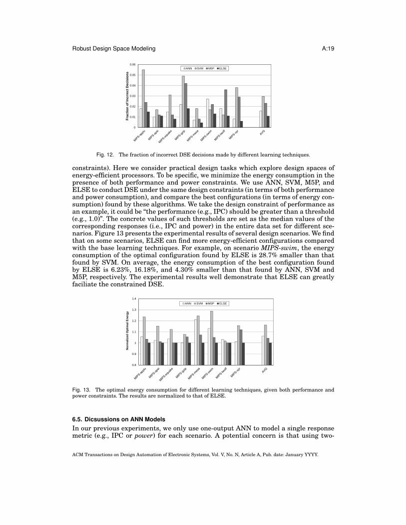
Figure 12 compares different learning techniques for several benchmarks runningon the MIPS architecture. Although ELSE does not outperform ANN on scenarioMIPS-apsi, it outperforms the base learning techniques on other 7 evaluated scenarios.On average, we observe that ELSE reduces incorrect predictions by 30.80%, 63.51%,and 53.24% compared with ANN, SVM and M5P, respectively. Therefore, ELSE is veryhelpful for iterative DSE compared with the base learning techniques.

The second usage scenario we considered is the constrained design space explo-ration, a DSE process factors in design constraints (e.g., performance/power/energy



0

0.01

0.02

0.03

0.04

0.05

0.06

Frac

tion

of In

crre

ct D

ecis

ions

ANN SVM M5P ELSE

Fig. 12. The fraction of incorrect DSE decisions made by different learning techniques.

constraints). Here we consider practical design tasks which explore design spaces ofenergy-efficient processors. To be specific, we minimize the energy consumption in thepresence of both performance and power constraints. We use ANN, SVM, M5P, andELSE to conduct DSE under the same design constraints (in terms of both performanceand power consumption), and compare the best configurations (in terms of energy con-sumption) found by these algorithms. We take the design constraint of performance asan example, it could be “the performance (e.g., IPC) should be greater than a threshold(e.g., 1.0)”. The concrete values of such thresholds are set as the median values of thecorresponding responses (i.e., IPC and power) in the entire data set for different sce-narios. Figure 13 presents the experimental results of several design scenarios. We findthat on some scenarios, ELSE can find more energy-efficient configurations comparedwith the base learning techniques. For example, on scenario MIPS-swim, the energyconsumption of the optimal configuration found by ELSE is 28.7% smaller than thatfound by SVM. On average, the energy consumption of the best configuration foundby ELSE is 6.23%, 16.18%, and 4.30% smaller than that found by ANN, SVM andM5P, respectively. The experimental results well demonstrate that ELSE can greatlyfaciliate the constrained DSE.

0.8

0.9

1

1.1

1.2

1.3

1.4

Nor

mal

ized

Opt

imal

Ene

rgy

ANN SVM M5P ELSE

Fig. 13. The optimal energy consumption for different learning techniques, given both performance andpower constraints. The results are normalized to that of ELSE.

6.5. Dicsussions on ANN ModelsIn our previous experiments, we only use one-output ANN to model a single responsemetric (e.g., IPC or power) for each scenario. A potential concern is that using two-


A:20 Q. Guo et al.

output ANN to simultaneously predict the IPC and power would achieve better accu-racy, since such response metrics are not independent. To address this concern, we alsobuild ANN with two outputs, and then compare their accuracy with two ANNs, eachwith only one output (i.e., one ANN for predicting IPC and the other for predictingpower) for several programs. Figure 14 shows the experimental results. On the evalu-ated benchmarks, it can be observed that the prediction accuracy of two-output ANNcannot always be improved. For example, the two-output ANN is only better than theone-output ANN for program equake and mesa when predicting IPC. When predictingpower, one-output ANN even outperforms two-output ANN for all evaluated programs.Therefore, the two-output ANN may not always be better than the one-output ANN.

Prediction Accuracy of ANN for IPC

Norm

ziled

MSE

0.00

0.20

0.40

0.60

0.80

1.00

1.20

equake gcc gzip mesa

1 Output Node 2 Output Nodes

Prediction Accuracy of ANN for Power

Norm

alize

d M

SE

0.00

0.25

0.50

0.75

1.00



Prediction Accuracy of ANN for IPC

Norm

ziled

MSE

0.00

0.20

0.40

0.60

0.80

1.00

1.20



Prediction Accuracy of ANN for Power

Norm

alize

d M

SE

0.00

0.25

0.50

0.75

1.00



Fig. 14. Comparison of prediction accuracy of one-output ANN and two-output ANN. The prediction error(i.e., MSE) is normalized to the results of two-output ANN.

7. CONCLUSIONArchitectural design space exploration is a very challenging task during the designof microprocessors, and learning/regression techniques are very promising to combattime-consuming simulations. However, according to detailed evaluations of existingtechniques on 52 different modeling tasks, we found that the accuracy variability ofexisting regression models is common and significant, and previous techniques are notrobust enough to offer reliable predictions for many different modeling tasks. To ad-dress the issue which may potentially diminish the general applicability of learningtechniques in EDSM, we suggest a EDSM framework called ELSE that employs mul-tiple base regression models to gain robustness. Like the stacking algorithm [Wolpert1992] that inspires our investigation, ELSE is an open framework that does not relyon any specific learning techniques, thus can be utilized to enhance the robustness oftraditional EDSM techniques. Experimental results show that ELSE can reduce about62% accuracy variability in comparison with the widely used ANN technique, enablingrobust EDSM that can adapt to different modeling tasks. Furthermore, ELSE can sig-nificantly reduce the prediction error for different modeling tasks.

In this paper, we mainly focus on performance modeling of a single benchmark,while multi-programmed applications are very common on existing multi-core archi-tectures. In the future, we plan to apply ELSE to the performance modeling of multi-programmed applications on multi-core architectures.

REFERENCESAZIZI, O., MAHESRI, A., LEE, B. C., PATEL, S. J., AND HOROWITZ, M. 2010. Energy-performance tradeoffs

in processor architecture and circuit design: a marginal cost analysis. In Proceedings of the 37th annualinternational symposium on Computer architecture. ISCA ’10. 26–36.



BROOKS, D., TIWARI, V., AND MARTONOSI, M. 2000. Wattch: a framework for architectural-level poweranalysis and optimizations. In Proceedings of the 27th annual international symposium on Computerarchitecture. ISCA ’00. 83–94.

BUJA, A. AND STUETZLE, W. 2000. The effect of bagging on variance, bias, and mean squared error. Tech-nical Report: AT&T Labs-Research.

CHO, C.-B., ZHANG, W., AND LI, T. 2007. Informed microarchitecture design space exploration using work-load dynamics. In Proceedings of the 40th Annual IEEE/ACM International Symposium on Microarchi-tecture. MICRO 40. 274–285.

DIETTERICH, T. G. 1998. Machine-learning research: Four current directions. The AI Magazine 18, 97–136.DUBACH, C., JONES, T., AND O’BOYLE, M. 2007. Microarchitectural design space exploration using an

architecture-centric approach. In Proceedings of the 40th Annual IEEE/ACM International Symposiumon Microarchitecture. MICRO 40. 262–271.

DUBACH, C., JONES, T. M., AND O’BOYLE, M. F. 2008. Exploring and predicting the architecture/optimisingcompiler co-design space. In Proceedings of the 2008 international conference on Compilers, architecturesand synthesis for embedded systems. CASES ’08. 31–40.

ELMOUSTAPHA OULD-AHMED-VALL, JAMES WOODLEE, C. Y. AND DOSHI, K. A. 2007. On the comparisonof regression algorithms for computer architecture performance analysis of software applications. InProceedings of the First Workshop on Statistical and Machine learning approaches applied to ARchitec-tures and compilaTion. SMART.

FRIEDMAN, J., HASTIE, T., AND TIBSHIRANI, R. 2000. Additive logistic regression: a statistical view ofboosting. Annals of Statistics 2, 337–407.

GUO, Q., CHEN, T., CHEN, Y., ZHOU, Z.-H., HU, W., AND XU, Z. 2011. Effective and efficient microprocessordesign space exploration using unlabeled design configurations. In Proceedings of the Twenty-SecondInternational Joint Conference on Artificial Intelligence - Volume Volume Two. IJCAI’11.

HARDAVELLAS, N., FERDMAN, M., FALSAFI, B., AND AILAMAKI, A. 2011. Toward dark silicon in servers.IEEE Micro 31, 4, 6–15.

IPEK, E., MCKEE, S. A., CARUANA, R., DE SUPINSKI, B. R., AND SCHULZ, M. 2006. Efficiently exploringarchitectural design spaces via predictive modeling. In Proceedings of the 12th international conferenceon Architectural support for programming languages and operating systems. ASPLOS XII. 195–206.

JOSEPH, P. J., VASWANI, K., AND THAZHUTHAVEETIL, M. J. 2006. A predictive performance model forsuperscalar processors. In Proceedings of the 39th Annual IEEE/ACM International Symposium onMicroarchitecture. MICRO 39. 161–170.

KHAN, S., XEKALAKIS, P., CAVAZOS, J., AND CINTRA, M. 2007. Using predictivemodeling for cross-programdesign space exploration in multicore systems. In Proceedings of the 16th International Conference onParallel Architecture and Compilation Techniques. PACT ’07. 327–338.

KUNCHEVA, L. 2002. A theoretical study on six classifier fusion strategies. IEEE Transactions on PatternAnalysis and Machine Intelligence 24, 2, 281 –286.

LEE, B. C. AND BROOKS, D. 2010. Applied inference: Case studies in microarchitectural design. ACM Trans.Archit. Code Optim. 7.

LEE, B. C. AND BROOKS, D. M. 2006. Accurate and efficient regression modeling for microarchitecturalperformance and power prediction. In Proceedings of the 12th international conference on Architecturalsupport for programming languages and operating systems. ASPLOS XII. 185–194.

LEE, B. C., COLLINS, J., WANG, H., AND BROOKS, D. 2008. Cpr: Composable performance regression forscalable multiprocessor models. In Proceedings of the 41st annual IEEE/ACM International Symposiumon Microarchitecture. MICRO 41. 270–281.

LIAO, S.-W., HUNG, T.-H., NGUYEN, D., CHOU, C., TU, C., AND ZHOU, H. 2009. Machine learning-basedprefetch optimization for data center applications. In Proceedings of the Conference on High PerformanceComputing Networking, Storage and Analysis. SC ’09.

MARIANI, G., PALERMO, G., ZACCARIA, V., AND SILVANO, C. 2013. Design-space exploration and runtimeresource management for multicores. ACM Trans. Embed. Comput. Syst. 13, 2, 20:1–20:27.

MOUDGILL, M., WELLMAN, J.-D., AND MORENO, J. H. 1999. Environment for powerpc microarchitectureexploration. IEEE Micro 19, 3, 15–25.

OPITZ, D. AND MACLIN, R. 1999. Popular ensemble methods: an empirical study. Journal of Artificial Intel-ligence Research 11, 169–198.

OULD-AHMED-VALL, E., WOODLEE, J., YOUNT, C., DOSHI, K. A., AND ABRAHAM, S. 2007. Using modeltrees for computer architecture performance analysis of software applications. In Proceedings of Inter-national Symposium on Performance Analysis of Systems and Software. ISPASS. 116–125.


A:22 Q. Guo et al.

PALERMO, G., SILVANO, C., AND ZACCARIA, V. 2009. Respir: A response surface-based pareto itera-tive refinement for application-specific design space exploration. Trans. Comp.-Aided Des. Integ. Cir.Sys. 28, 12.

PAONE, E., VAHABI, N., ZACCARIA, V., SILVANO, C., MELPIGNANO, D., HAUGOU, G., AND LEPLEY, T. 2013.Improving simulation speed and accuracy for many-core embedded platforms with ensemble models. InProceedings of the Conference on Design, Automation and Test in Europe. DATE ’13.

RENAU, J., FRAGUELA, B., TUCK, J., LIU, W., PRVULOVIC, M., CEZE, L., SARANGI, S., SACK, P., STRAUSS,K., AND MONTESINOS, P. 2005. SESC simulator. http://sesc.sourceforge.net.

SCHAPIRE, R. E. 1990. The strength of weak learnability. Machine Learning 5, 197–227.TARJAN, D., THOZIYOOR, S., AND JOUPPI, N. P. 2006. Cacti 4.0. Technical Report: HPL-2006-86.VAPNIK, V. N. 1995. The Nature of Statistical Learning Theory. Springer-Verlag New York, Inc.WANG, Y. AND WITTEN, I. H. 1997. Induction of model trees for predicting continuous classes. In Proceed-

ings of European Conference on Machine Learning (ECML). ECML’97.WITTEN, I. H. AND FRANK, E. 2005. Data Mining: Practical Machine Learning Tools and Techniques with

Java Implementations 2nd Edition Ed. Morgan Kaufmann.WOLPERT, D. 1997. The lack of a priori distinctions between learning algorithms. Neural Computation 8, 7,

1341–1390.WOLPERT, D. AND MACREADY, W. G. 1997. No free lunch theorems for optimization. IEEE Transactions on

Evolutionary Computation 1, 1, 67–82.WOLPERT, D. H. 1992. Stacked generalization. Neural Networks 5, 241–259.YI, J. J., EECKHOUT, L., LILJA, D. J., CALDER, B., JOHN, L. K., AND SMITH, J. E. 2006. The future of

simulation: A field of dreams. Computer 39, 22–29.ZHOU, Z.-H. 2012. Ensemble Methods: Foundations and Algorithms. Boca Raton, FL: Chapman & Hall/CRC.


Documents

A Robust Design Space Modeling - cs.nju.edu.cn