A Risk-centric Model of Demand Recessions and Speculation∗

Ricardo J. Caballero Alp Simsek

This draft: July 22, 2019

Abstract

We theoretically analyze the interactions between asset prices, financial speculation, and

macroeconomic outcomes when output is determined by aggregate demand. If the interest rate

is constrained, a decline in risky asset valuations generates a demand recession. This reduces

earnings and generates a negative feedback loop between asset prices and aggregate demand.

In the recession phase, beliefs matter not only because they affect asset valuations but also

because they determine the strength of the amplification mechanism. In the ex-ante boom phase,

belief disagreements (or heterogeneous asset valuations) matter because they induce investors to

speculate. This speculation exacerbates the crash by reducing high-valuation investors’wealth

when the economy transitions to recession. Macroprudential policy that restricts speculation in

the boom can Pareto improve welfare by increasing asset prices and aggregate demand in the

recession.

JEL Codes: E00, E12, E21, E22, E30, E40, G00, G01, G11Keywords: Asset prices, aggregate demand, time-varying risk premium, exogenous and

endogenous uncertainty, interest rate rigidity, booms and recessions, heterogeneous beliefs,

speculation, monetary and macroprudential policy, the Fed put

Dynamic link to the most recent draft:https://www.dropbox.com/s/ud0jejruqxsc852/DRSR_37_public.pdf?dl=0

∗Contact information: Caballero (MIT and NBER; caball@mit.edu) and Simsek (MIT, NBER, and CEPR; asim-sek@mit.edu). A previous version of the paper was circulated under the title, “A Risk-centric Model of DemandRecessions and Macroprudential Policy.” Chris Ackerman, Masao Fukui, Jeremy Majerovitz, Andrea Manera, ZiluPan, Olivier Wang, and Nathan Zorzi provided excellent research assistance. We also thank Jaroslav Borovicka,Emmanuel Farhi, Kristin Forbes, Mark Gertler, Zhiguo He, Yueran Ma, Plamen Nenov, Matthew Rognlie, Mar-tin Schneider, Larry Summers, Jaume Ventura, and seminar participants at Yale University, Columbia University,Boston College, MIT, Princeton University, the EIEF, Paris School of Economics, the BIS, the Bank of Spain, the FedBoard, the Boston Fed; as well as conference participants at the CCBS Conference hosted by the Bank of Englandand MacCalm, the Wharton Conference on Liquidity and Financial Fragility, the Harvard/MIT Financial EconomicsWorkshop, Cowles Conference on General Equilibrium and Applications, NBER meetings (EFG, AP, and SI Impulseand Propagation Mechanisms), AEA annual meetings (2018 and 2019), CEBRA annual meeting, the Barcelona GSEConference on Asset Pricing and Macroeconomics, the Sciences Po Summer Workshop in International and MacroFinance for their comments. Simsek acknowledges support from the National Science Foundation (NSF) under GrantNumber SES-1455319. First draft: May 11, 2017.

1. Introduction

Prices of risky assets, such as stocks and houses, fluctuate considerably without meaningful changes

in underlying payoffs. These fluctuations, which are due to a host of rational and behavioral

mechanisms, are generically described as the result of a “time-varying risk premium”(see, Cochrane

(2011); Shiller et al. (2014) and Campbell (2014) for recent reviews). While fluctuations in risky

asset prices affect the macroeconomy in a multitude of ways, a growing empirical literature suggests

that aggregate demand plays a central role and therefore interest rate policy can mitigate the impact

of asset price shocks (see Pflueger et al. (2018) for evidence that prices of volatile stocks have high

predictive power for economic activity and interest rates).1 A current policy concern is that, with

interest rates close to their effective lower bound in much of the developed world, interest rate

policy will be unable to respond to future large negative asset price shocks.

This connection between risky asset prices and aggregate demand highlights that speculation– a

pervasive feature of financial markets driven by heterogeneous asset valuations– can lead to more

severe downturns. There is in fact an old tradition in macroeconomics that emphasizes speculation

as a central feature of asset prices in boom-bust cycles (see, e.g., Minsky (1977); Kindleberger

(1978)). In recent empirical work, Mian and Sufi (2018) argue that speculation also played a key

role in the U.S. housing cycle. However, speculation and its interaction with aggregate demand

are largely missing from the modern macroeconomic theory connecting asset prices with economic

activity, which mostly focuses on financial frictions (see Gertler and Kiyotaki (2010) for a review).

This omission is especially important in the current low interest rates environment, as monetary

policy has little space to mop up a sharp decline in risky asset prices following a speculative episode.

In this paper, we build a risk-centric macroeconomic model– that is, a model in which risky asset

prices play an important role– with the two key features highlighted above. First, we emphasize

the role of the aggregate demand channel and interest rate frictions in causing recessions driven by

a rise in the “risk premium”– our catchall phrase for shocks to asset valuations. Second, we study

the impact of financial speculation on the severity of these recessions and derive the implications

for macroprudential policy. In order to isolate our insights, we remove all financial frictions.

Our model is set in continuous time with diffusion productivity shocks and Poisson shocks that

move the economy between high and low risk premium states. The supply side is a stochastic

endowment economy with sticky prices (which we extend to an endogenous growth model when

we add investment). The demand side has risk-averse consumer-investors who demand goods and

risky assets. We focus on “interest rate frictions” and “financial speculation.” By interest rate

frictions, we mean factors that might constrain or delay the adjustment of the risk-free interest

rate to shocks. For concreteness, we work with a zero lower bound on the policy interest rate, but

our mechanism is also applicable with other interest rate constraints such as a currency union or a

fixed exchange rate. By financial speculation, we mean the trading of risky financial assets among

investors that have heterogeneous valuations for these assets. We capture speculation by allowing

1Cieslak and Vissing-Jorgensen (2017) conduct a textual analysis of FOMC minutes and show that the Fed paysattention to stock prices and cuts interest rates after stock price declines (“the Fed put”).

1

Figure 1: Output-asset price feedbacks during a risk-centric demand recession.

investors to have belief disagreements with respect to the transition probabilities between high and

low risk premium states.

To fix ideas, consider an increase in perceived volatility (equivalently, an increase in average

pessimism). This is a “risk premium shock” that exerts downward pressure on risky asset prices

without a change in current productivity (the supply-determined output level). If the monetary

authority allows asset prices to decline, then low prices induce a recession by reducing aggregate

demand through a wealth effect. Consequently, monetary policy responds by reducing the interest

rate, which stabilizes asset prices and aggregate demand. However, if the interest rate is constrained,

the economy loses its natural line of defense. In this case, the rise in the risk premium reduces

asset prices and generates a demand recession.

Dynamics play a crucial role in this environment, as the recession is exacerbated by feedback

mechanisms. In the main model, when investors expect the higher risk premium to persist, the

decline in future demand lowers expected earnings, which exerts further downward pressure on

asset prices. With endogenous investment, there is a second mechanism, as the decline in current

investment lowers the growth of potential output, which further reduces expected earnings and asset

prices. In turn, the decline in asset prices feeds back into current consumption and investment,

generating scope for severe spirals in asset prices and output. Figure 1 illustrates these dynamic

mechanisms. The feedbacks are especially powerful when investors are pessimistic and think the

higher risk premium will persist. Hence, beliefs matter in our economy not only because they have

a direct impact on asset prices but also because they determine the strength of the amplification

mechanism.

2

In this environment, speculation during the low risk premium phase (boom) exacerbates the

recession when there is a transition to the high risk premium phase. With heterogeneous asset

valuations, which we capture with belief disagreements about state transition probabilities, the

economy’s degree of optimism depends on the wealth share of optimists (or high-valuation in-

vestors). During recessions, the economy benefits from wealthy optimists because they raise asset

valuations, increasing aggregate demand. However, disagreements naturally lead to speculation

during booms, which depletes optimists’wealth during recessions. Specifically, optimists take on

risk by selling insurance contracts to pessimists that enrich optimists if the boom persists but lead

to a large reduction in their wealth share when there is a transition to recession. This reallocation

of wealth lowers asset prices and leads to a more severe recession.

These effects motivate macroprudential policy that restricts speculation during the boom. We

show that macroprudential policy that makes optimistic investors behave as-if they were more pes-

simistic (implemented via portfolio risk limits) can generate a Pareto improvement in social welfare.

This result is not driven by paternalistic concerns– the planner respects investors’own beliefs, and

the result does not depend on whether optimists or pessimists are closer to the truth. Rather, the

planner improves welfare by internalizing aggregate demand externalities. The depletion of opti-

mists’wealth during a demand recession depresses asset prices and aggregate demand. Optimists

(or more broadly, high-valuation investors) do not internalize the effect of their risk taking on as-

set prices and aggregate demand during the recession. This leads to excessive risk taking that is

corrected by macroprudential policy. Moreover, our model supports procyclical macroprudential

policy. While macroprudential policy can be useful during the recession, these benefits can be

outweighed by its immediate negative impact on asset prices. This decline can be offset by the

interest rate policy during the boom but not during the recession.

While there is an extensive empirical literature supporting the components of our model (see

Section 7 for a brief summary), we extend this literature by presenting empirical evidence consistent

with our results. We focus on three implications. First, our model predicts that shocks to asset

valuations generate a more severe demand recession when the interest rate is constrained. Second,

the recession reduces firms’ earnings and leads to a further decline in asset prices. Third, the

recession is more severe when the shock takes place in an environment with more speculation.

To investigate these predictions, we assemble a quarterly panel data set of 21 advanced countries

between 1990 and 2017, and subdivide the panel into countries that are part of the Eurozone or

the European Exchange Rate Mechanism (the Euro/ERM sample) and those that have their own

currencies (the non-Euro/ERM sample). Countries in the first group have a constrained interest

rate with respect to local asset price shocks, since they share a common monetary policy. The

second group has a less constrained interest rate. We find that a negative house price shock in

a non-Euro/ERM country is associated with an initial decline in economic activity, followed by

a decline in the policy interest rate and output stabilization. In contrast, a similar shock in a

Euro/ERM country is associated with no interest rate response (compared to other Euro/ERM

countries), which is followed by a more persistent and larger decline in economic activity. We also

3

find that the house price shock is followed by a larger decline in earnings and stock prices of publicly

traded firms in the Euro/ERM sample (although the standard errors are larger for these results).

Finally, we find that past bank credit expansion– which we use as a proxy for speculation on house

prices– is associated with more severe outcomes following the house price shock in the Euro/ERM

sample (but not in the other sample).

Literature review. Our paper is related to three main literatures: two in macroeconomics and

one in finance. On the macroeconomics side, a large body of work emphasizes the links between

asset prices and macroeconomic outcomes. Our model contributes to this literature by establishing

a relationship between asset prices and aggregate demand even without financial frictions. This

relates our paper to strands of the New-Keynesian literature that emphasize demand shocks that

might drive business cycles while also affecting asset prices, such as “news shocks”(Beaudry and

Portier (2006)), “noise shocks” (Lorenzoni (2009); Blanchard et al. (2013)), “confidence shocks”

(Ilut and Schneider (2014)), “uncertainty shocks”(Basu and Bundick (2017); Fernández-Villaverde

et al. (2015)), and “disaster shocks” (Isoré and Szczerbowicz (2017)). Aside from the modeling

novelty (ours is a continuous time macrofinance model), we provide an integrated treatment of these

and related forces. We refer to them as “risk premium shocks”to emphasize their close connection

with asset prices and the finance literature on time-varying risk premia. Accordingly, we make asset

prices the central object in our analysis, breaking with convention in the New-Keynesian literature

without financial frictions.2 More substantively, we show that heterogeneity in asset valuation

matters in these environments. This heterogeneity matters because it leads to speculation that

exacerbates demand recessions and provides a distinct rationale for macroprudential regulation.

Another important macroeconomics literature focuses on uncertainty and its role in driving

macroeconomic fluctuations (e.g., Bloom (2009); Baker et al. (2016); Bloom et al. (2018)). We

contribute to this literature by showing how uncertainty affects aggregate activity through asset

prices and their impact on aggregate demand. We also illustrate how uncertainty shocks have

stronger effects when monetary policy is constrained, consistent with recent empirical evidence

(e.g., Plante et al. (2018)). Finally, we show that ex-ante financial speculation amplifies the damage

from uncertainty shocks.

On the finance side, a large literature emphasizes investors’ beliefs as a key driver of finan-

cial boom-bust cycles (see, e.g., Gennaioli and Shleifer (2018) for the role of beliefs in the recent

crisis). A strand of this literature argues that heterogeneity in the degree of optimism combined

with short-selling constraints can lead to speculative asset price bubbles that substantially amplify

the financial cycle (e.g., Harrison and Kreps (1978); Scheinkman and Xiong (2003); Geanakoplos

(2010); Simsek (2013a); Barberis et al. (2018)). Related contributions emphasize that disagree-

ments exacerbate asset price fluctuations more broadly– even without short-selling constraints or

bubbles– because they create endogenous fluctuations in agents’wealth distribution (e.g., Basak

(2000, 2005); Detemple and Murthy (1994); Zapatero (1998); Cao (2017); Xiong and Yan (2010);

2For an exception, see Galí (2018) who develops an OLG variant of the New-Keynesian model with rational bubbles(see also Biswas et al. (2018)).

4

Kubler and Schmedders (2012); Korinek and Nowak (2016)). Our paper features similar forces but

explores them in an environment where output is not necessarily at its supply-determined level. We

show that speculation during the boom not only worsens the asset price bust but also exacerbates

the demand recession. Consequently, and unlike much of this literature, macroprudential policy

that restricts speculation can improve welfare even if the planner is not paternalistic and respects

investors’(heterogeneous and possibly over-optimistic) beliefs. Adding paternalistic concerns would

reinforce our normative conclusions (see Section 6).3

The interactions between heterogeneous valuations, risk-premia, and interest rate lower bounds

are central themes of the literature on structural safe asset shortages and safety traps (see, for

instance, Caballero and Farhi (2017); Caballero et al. (2017b)). Aside from emphasizing a broader

set of factors that can drive the risk premium (in addition to safe asset scarcity), we contribute to

this literature by focusing on dynamics. We analyze the connections between boom and recession

phases of recurrent business cycles driven by risk premium shocks. We show that speculation

between “optimists” and “pessimists”during the boom exacerbates a future risk-centric demand

recession, and derive the implications for macroprudential policy. In contrast, Caballero and Farhi

(2017) show how “pessimists”can create a demand recession in otherwise normal times and derive

the implications for fiscal policy and unconventional monetary policy.4

At a methodological level, our paper belongs to the new continuous time macrofinance literature

started by the work of Brunnermeier and Sannikov (2014, 2016a) and summarized in Brunnermeier

and Sannikov (2016b) (see also Basak and Cuoco (1998); Adrian and Boyarchenko (2012); He and

Krishnamurthy (2012, 2013); Di Tella (2017, 2019); Moreira and Savov (2017); Silva (2016)). This

literature highlights the full macroeconomic dynamics induced by financial frictions. While the

structure of our economy shares many features with theirs, our model has no financial frictions,

and the macroeconomic dynamics stem not from the supply side (relative productivity) but from

the aggregate demand side.

Our results on macroprudential policy are related to recent work that analyzes the implications

of aggregate demand externalities for the optimal regulation of financial markets. For instance,

Korinek and Simsek (2016) show that, in the run-up to deleveraging episodes that coincide with a

zero-lower-bound on the interest rate, policies targeted at reducing household leverage can improve

welfare (see also Farhi and Werning (2017)). In these papers, macroprudential policy works by

reallocating wealth across agents and states so that agents with a higher marginal propensity to

consume hold relatively more wealth when the economy is depressed due to deficient demand. The

mechanism in our paper is different and works through heterogeneous asset valuations. The policy

operates by transferring wealth to optimists during recessions, not because optimists spend more

3More broadly, our paper is part of a large finance literature that investigates the effect of belief disagreementsand speculation on financial markets (e.g., Lintner (1969); Miller (1977); Varian (1989); Harris and Raviv (1993);Chen et al. (2002); Fostel and Geanakoplos (2008); Simsek (2013b); Iachan et al. (2015)).

4Our paper is also related to an extensive literature on liquidity traps that has exploded since the Great Recession(see, for instance, Tobin (1975); Krugman (1998); Eggertsson and Woodford (2006); Guerrieri and Lorenzoni (2017);Werning (2012); Hall (2011); Christiano et al. (2015); Rognlie et al. (2018); Midrigan et al. (2016); Bacchetta et al.(2016)).

5

than other investors, but because they raise asset valuations and induce all investors to spend more

(while also increasing aggregate investment).5

The macroprudential literature beyond aggregate demand externalities is mostly motivated by

the presence of pecuniary externalities that make the competitive equilibrium constrained ineffi cient

(e.g., Caballero and Krishnamurthy (2003); Lorenzoni (2008); Bianchi and Mendoza (2018); Jeanne

and Korinek (2018)). The friction in this literature is market incompleteness or collateral constraints

that depend on asset prices (see Davila and Korinek (2016) for a detailed exposition). We show

that a decline in asset prices is damaging not only for the reasons emphasized in this literature,

but also because it lowers aggregate demand.

The rest of the paper is organized as follows. In Section 2 we present an example that illustrates

the main mechanism and motivates the rest of our analysis. Section 3 presents the general environ-

ment and defines the equilibrium. Section 4 characterizes the equilibrium in a benchmark setting

with common beliefs and homogeneous asset valuations. This section shows how risk premium

shocks can lower asset prices and induce a demand recession, and how the recession is exacerbated

by feedback loops between asset prices and aggregate demand. Section 5 characterizes the equilib-

rium with belief disagreements and heterogeneous asset valuations, and illustrates how speculation

exacerbates the recession. Section 6 shows the aggregate demand externalities associated with op-

timists’risk taking and establishes our results on macroprudential policy. Section 7 presents our

empirical analysis and summarizes supporting evidence from the related literature. Section 8 con-

cludes. The (online) appendices contain the omitted derivations and proofs as well as the details

of our empirical analysis.

2. A stepping-stone example

Here we present a simple (largely static) example that serves as a stepping stone into our main

(dynamic) model. We start with a representative agent setup and illustrate the basic aggregate

demand mechanism. We then consider belief disagreements and illustrate the role of speculation.

A two-period risk-centric aggregate demand model. Consider an economy with two dates,

t ∈ {0, 1}, a single consumption good, and a single factor of production– capital. For simplicity,capital is fixed (i.e., there is no depreciation or investment) and it is normalized to one. Potential

output is equal to capital’s productivity, zt, but the actual output can be below this level due to a

shortage of aggregate demand, yt ≤ zt. For simplicity, we assume output is equal to its potential atthe last date, y1 = z1, and focus on the endogenous determination of output at the previous date,

y0 ≤ z0. We assume the productivity at date 1 is uncertain and log-normally distributed so that,

log y1 = log z1 ∼ N(g − σ2

2, σ2). (1)

5See Farhi and Werning (2016) for a synthesis of some of the key mechanisms that justify macroprudential policiesin models that exhibit aggregate demand externalities.

6

We also normalize the initial productivity to one, z0 = 1, so that g captures the (log) expected

growth rate of productivity, and σ captures its volatility.

There are two types of assets. There is a “market portfolio”that represents claims to the output

at date 1 (which accrue to production firms as earnings), and a risk-free asset in zero net supply.

We denote the price of the market portfolio with Q, and its log return with,

rm (z1) = logz1Q. (2)

We denote the log risk-free interest rate with rf .

For now, the demand side is characterized by a representative investor, who is endowed with the

initial output as well as the market portfolio (we introduce disagreements at the end of the section).

At date 0, she chooses how much to consume, c0, and what fraction of her wealth to allocate to

the market portfolio, ωm (with the residual fraction invested in the risk-free asset). When asset

markets are in equilibrium, she will allocate all of her wealth to the market portfolio, ωm = 1, and

her portfolio demand will determine the risk premium.

We assume the investor has Epstein-Zin preferences with the discount factor, e−ρ, and the

relative risk aversion coeffi cient (RRA), γ. For simplicity, we set the elasticity of intertemporal

substitution (EIS) equal to 1. Later in this section, we will show that relaxing this assumption

leaves our conclusions qualitatively unchanged. In the dynamic model, we will simplify the analysis

further by setting RRA as well as EIS equal to 1 (which leads to time-separable log utility).

The supply side of the economy is described by New-Keynesian firms that have pre-set fixed

prices. These firms meet the available demand at these prices as long as they are higher than their

marginal cost (see Appendix B.1.2 for details). These features imply that output is determined by

the aggregate demand for goods (consumption) up to the capacity constraint,

y0 = c0 ≤ z0. (3)

Since prices are fully sticky, the real interest rate is equal to the nominal interest rate, which is

controlled by the monetary authority. We assume that the interest rate policy attempts to replicate

the supply-determined output level. However, there is a lower bound constraint on the interest rate,

rf ≥ 0. Thus, the interest rate policy is described by, rf = max(rf∗, 0

), where rf∗ is the natural

interest rate that ensures output is at its potential, y0 = z0.

To characterize the equilibrium, first note that there is a tight relationship between output and

asset prices. Specifically, the assumption on the EIS implies that the investor consumes a fraction

of her lifetime income,

c0 =1

1 + e−ρ(y0 +Q) . (4)

Combining this expression with Eq. (3), we obtain the following equation,

y0 = eρQ. (5)

7

We refer to this equation as the output-asset price relation– generally, it is obtained by combining

the consumption function (and when there is investment, also the investment function) with goods

market clearing. The condition says that asset prices increase aggregate wealth and consumption,

which in turn leads to greater output.

Next, note that asset prices must also be consistent with equilibrium in risk markets. In

Appendix A.1, we show that, up to a local approximation, the investor’s optimal weight on the

market portfolio is determined by,

ωmσ ' 1

γ

E [rm (z1)] + σ2

2 − rf

σ. (6)

In words, the optimal portfolio risk (left side) is proportional to “the Sharpe ratio”on the market

portfolio (right side). The Sharpe ratio captures the reward per risk, where the reward is determined

by the risk premium: the (log) expected return in excess of the (log) risk free rate. This is the

standard risk-taking condition for mean-variance portfolio optimization, which applies exactly in

continuous time. It applies approximately in the two-period model, and the approximation becomes

exact when there is a representative household and the asset markets are in equilibrium (ωm = 1).

In particular, substituting the asset market clearing condition, ωm = 1, and the expected return

on the market portfolio from Eqs. (1) and (2), we obtain the following equation,

σ =1

γ

g − logQ− rfσ

. (7)

We refer to this equation as the risk balance condition– generally, it is obtained by combining

investors’optimal portfolio allocations with asset market clearing and the equilibrium return on

the market portfolio. It says that, the equilibrium level of the Sharpe ratio on the market portfolio

(right side) needs to be suffi ciently large to convince investors to hold the risk generated by the

productive capacity (left side).

Next, consider the supply-determined equilibrium in which output is equal to its potential,

y0 = z0 = 1. Eq. (5) reveals that this requires the asset price to be at a particular level, Q∗ = e−ρ.

Combining this with Eq. (7), the interest rate also needs to be at a particular level,

rf∗ = g + ρ− γσ2. (8)

Intuitively, the monetary policy needs to set the interest rate to a low enough level to induce

suffi ciently high asset prices and aggregate demand to clear the goods market.

Now suppose the initial parameters are such that rf∗ > 0, so that the equilibrium features

Q∗, rf∗ and supply-determined output, y0 = z0 = 1. Consider a “risk premium shock”that raises

the volatility, σ, or risk aversion, γ. The immediate impact of this shock is to create an imbalance

in the risk balance condition (7). The economy produces too much risk (left side) relative to what

investors are willing to absorb (right side). In response, the monetary policy lowers the risk-free

interest rate (as captured by the decline in rf∗), which increases the risk premium and equilibrates

8

the risk balance condition (7). Intuitively, the monetary authority lowers the opportunity cost of

risky investment and induces investors to absorb risk.

Next suppose the shock is suffi ciently large so that the natural interest rate becomes negative,

rf∗ < 0, and the actual interest rate becomes constrained, rf = 0. In this case, the risk balance

condition is re-established with a decline in the price of the market portfolio, Q. This increases the

expected return on risky investment, which induces investors to absorb risk. However, the decline

in Q reduces aggregate wealth and induces a demand-driven recession. Formally, we combine Eqs.

(5) and (7) to obtain,

log y0 = ρ+ logQ where logQ = g − γσ2. (9)

Note also that, in the constrained region, asset prices and output become sensitive to beliefs about

future prospects. For instance, a decrease in the expected growth rate, g (pessimism)– rational or

otherwise– decreases asset prices and worsens the recession. In fact, while we analyzed shocks that

raise σ or γ, Eqs. (8) and (9) reveal that shocks that lower g lead to the same effects.

More general EIS. Now consider the same model with the difference that we allow the EIS,

denoted by ε, to be different than one. Appendix A.2 analyzes this case and shows that the analogue

of the output-asset price relation is given by [cf. Eq. (5)],

y0 = eρε(RCE

)1−εQ. (10)

Here, RCE denotes the investor’s certainty-equivalent portfolio return that we formally define in

the appendix. The expression follows from the fact that consumption is not only influenced by a

wealth effect, as in the baseline analysis, but also by substitution and income effects. When ε > 1,

the substitution effect dominates. All else equal, a decline in the attractiveness of investment

opportunities captured by a reduction in RCE tends to reduce savings and increase consumption,

which in turn increases output. Conversely, when ε < 1, the income effect dominates and a decline

in RCE tends to increase savings and reduce consumption and output.

We also show that the risk balance condition (7) remains unchanged (because the EIS does

not affect the investor’s portfolio problem). Furthermore, we derive the equilibrium level of the

certainty-equivalent return as,

logRCE = g − logQ− 1

2γσ2. (11)

As expected, RCE decreases with the volatility, σ, and the risk aversion, γ.

These expressions illustrate that a risk premium shock that increases σ or γ (or lowers g)

affects consumption and aggregate demand through two channels. As before, it exerts a downward

influence on asset prices, which reduces consumption through a wealth effect. But in this case

it also exerts a downward influence on the certainty-equivalent return, which affects consumption

9

further depending on the balance of income and substitution effects. When ε > 1, the second

channel works against the wealth effect because investors substitute towards consumption. When

ε < 1, the second channel reinforces the wealth effect.

In Appendix A.2, we complete the characterization of equilibrium and show that the net effect

on aggregate demand is qualitatively the same as in the baseline analysis regardless of the level

of EIS. In particular, a risk premium shock that increases γ or σ (or lowers g) reduces rf∗ (see

Eq. (A.9)).6 When the interest rate is constrained, rf = 0, the shock reduces the equilibrium

level of output y0, as well as the asset price, Q (see Eq. (A.10)). When ε > 1, the substitution

effect mitigates the magnitude of these declines but it does not overturn them– that is, the wealth

effect ultimately dominates. Since the purpose of our model is to obtain qualitative insights, in the

dynamic model we assume ε = 1 and isolate the wealth effect.7

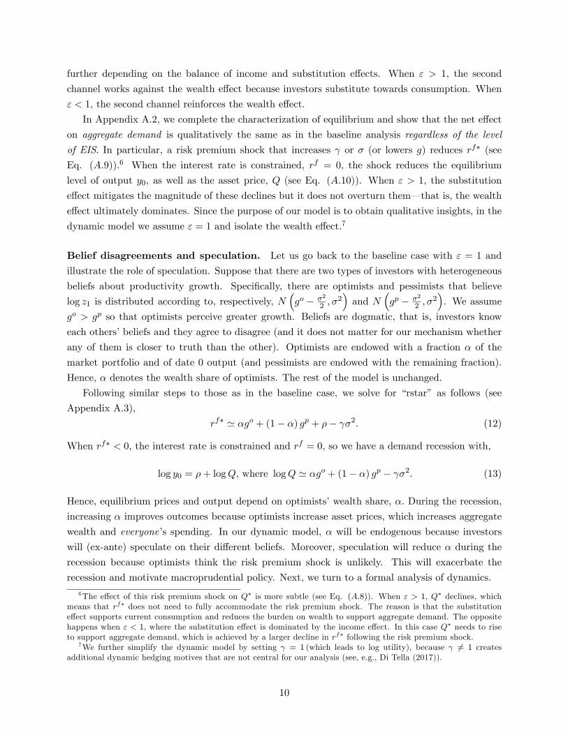
Belief disagreements and speculation. Let us go back to the baseline case with ε = 1 and

illustrate the role of speculation. Suppose that there are two types of investors with heterogeneous

beliefs about productivity growth. Specifically, there are optimists and pessimists that believe

log z1 is distributed according to, respectively, N(go − σ2

2 , σ2)and N

(gp − σ2

2 , σ2). We assume

go > gp so that optimists perceive greater growth. Beliefs are dogmatic, that is, investors know

each others’beliefs and they agree to disagree (and it does not matter for our mechanism whether

any of them is closer to truth than the other). Optimists are endowed with a fraction α of the

market portfolio and of date 0 output (and pessimists are endowed with the remaining fraction).

Hence, α denotes the wealth share of optimists. The rest of the model is unchanged.

Following similar steps to those as in the baseline case, we solve for “rstar” as follows (see

Appendix A.3),

rf∗ ' αgo + (1− α) gp + ρ− γσ2. (12)

When rf∗ < 0, the interest rate is constrained and rf = 0, so we have a demand recession with,

log y0 = ρ+ logQ, where logQ ' αgo + (1− α) gp − γσ2. (13)

Hence, equilibrium prices and output depend on optimists’wealth share, α. During the recession,

increasing α improves outcomes because optimists increase asset prices, which increases aggregate

wealth and everyone’s spending. In our dynamic model, α will be endogenous because investors

will (ex-ante) speculate on their different beliefs. Moreover, speculation will reduce α during the

recession because optimists think the risk premium shock is unlikely. This will exacerbate the

recession and motivate macroprudential policy. Next, we turn to a formal analysis of dynamics.

6The effect of this risk premium shock on Q∗ is more subtle (see Eq. (A.8)). When ε > 1, Q∗ declines, whichmeans that rf∗ does not need to fully accommodate the risk premium shock. The reason is that the substitutioneffect supports current consumption and reduces the burden on wealth to support aggregate demand. The oppositehappens when ε < 1, where the substitution effect is dominated by the income effect. In this case Q∗ needs to riseto support aggregate demand, which is achieved by a larger decline in rf∗ following the risk premium shock.

7We further simplify the dynamic model by setting γ = 1 (which leads to log utility), because γ 6= 1 createsadditional dynamic hedging motives that are not central for our analysis (see, e.g., Di Tella (2017)).

10

3. Dynamic environment and equilibrium

In this section we first introduce our general dynamic environment and define the equilibrium. We

then describe the optimality conditions and provide a partial characterization of equilibrium. In

subsequent sections we will further characterize this equilibrium in various special cases of interest.

Throughout, we simplify the analysis by abstracting away from investment. In Appendix D.1, we

extend the environment to introduce investment and endogenous growth. We discuss additional

results related to investment at the end of Section 4.

Potential output and risk premium shocks. The economy is set in infinite continuous time,

t ∈ [0,∞), with a single consumption good and a single factor of production, capital. Let kt,sdenote the capital stock at time t and in the aggregate state s ∈ S. Suppose that, when fully

utilized, kt,s units of capital produce Akt,s units of the consumption good. Hence, Akt,s denotes

the potential output in this economy. Capital follows the process,

dkt,skt,s

= gdt+ σsdZt. (14)

Here, g denotes the expected productivity growth, which is an exogenous parameter in the main

text (it is endogenized in Appendix D.1 that introduces investment). The term, dZt, denotes the

standard Brownian motion, which captures “aggregate productivity shocks.”8

The states, s ∈ S, differ only in terms of the volatility of aggregate productivity, σs. For

simplicity, there are only two states, s ∈ {1, 2}, with σ1 < σ2. State s = 1 corresponds to a

low-volatility state, whereas state s = 2 corresponds to a high-volatility state. At each instant, the

economy in state s transitions into the other state s′ 6= s according to a Poisson process. We use

these volatility shocks to capture the time variation in the risk premium due to various unmodeled

factors (see Section 2 for an illustration of how risk, risk aversion, or beliefs play a similar role in

our analysis).

Transition probabilities and belief disagreements. We let λis > 0 denote the perceived

Poisson transition probability in state s (into the other state) according to investor i ∈ I. Theseprobabilities capture the degree of investors’(relative) optimism or pessimism. For instance, greater

λi2 corresponds to greater optimism because it implies the investor expects the current high-risk-

premium conditions to end relatively soon. Likewise, smaller λi1 corresponds to greater optimism

because it implies the investor expects the current low-risk-premium conditions to persist longer.

Belief disagreements provide the only exogenous source of heterogeneity in our model. We first ana-

lyze the special case with common beliefs (Section 4) and then investigate belief disagreements and

8Note that fluctuations in kt,s generate fluctuations in potential output, Akt,s. We introduce Brownian shocks tocapital, kt,s, as opposed to total factor productivity, A, since this leads to a slightly more tractable analysis whenwe extend the model to include investment (see Appendix D). In the main text, we could equivalently introduce theshocks to A and conduct the analysis by normalizing all relevant variables with At,s as opposed to kt,s.

11

speculation (Section 5). When investors disagree, they have dogmatic beliefs (formally, investors

know each others’beliefs and they agree to disagree).

Menu of financial assets. There are three types of financial assets. First, there is a market

portfolio that represents a claim on all output (which accrues to production firms as earnings as we

describe later). We let Qt,skt,s denote the price of the market portfolio, so Qt,s denotes the price

per unit of capital. We let rmt,s denote the instantaneous expected return on the market portfolio

conditional on no transition. Second, there is a risk-free asset in zero net supply. We denote its

instantaneous return by rft,s. Third, in each state s, there is a contingent Arrow-Debreu security

that trades at the (endogenous) price ps′t,s and pays 1 unit of the consumption good if the economy

transitions into the other state s′ 6= s. This security is also in zero net supply and it ensures that

the financial markets are dynamically complete.

Price and return of the market portfolio. Absent transitions, the price per unit of capital

follows an endogenous but deterministic process,9

dQt,sQt,s

= µQt,sdt for s ∈ {1, 2} . (15)

Combining Eqs. (14) and (15), the price of the market portfolio (conditional on no transition)

evolves according to,d (Qt,skt,s)

Qt,skt,s=(g + µQt,s

)dt+ σsdZt.

This implies that, absent state transitions, the volatility of the market portfolio is given by σs, and

its expected return is given by,

rmt,s =yt,s

Qt,skt,s+ g + µQt,s. (16)

Here, yt,s denotes the endogenous level of output at time t. The first term captures the “dividend

yield” component of return. The second and third terms capture the (expected) capital gain

conditional on no transition, which reflects the expected growth of capital as well as of the price

per unit of capital.

Eqs. (15− 16) describe the prices and returns conditional on no state transition. If there is a

transition at time t from state s into state s′ 6= s, then the price per unit of capital jumps from Qt,s

to a potentially different level, Qt,s′ . Therefore, investors that hold the market portfolio experience

instantaneous capital gains or losses that are reflected in their portfolio problem.

9 In general, the price follows a diffusion process and this equation also features an endogenous volatility term,σQt,sdZt. In this model, we have σQt,s = 0 because we work with complete financial markets, constant elasticitypreferences, and no disagreements aside from the probability of state transitions. These features ensure that investorsallocate identical portfolio weights to the market portfolio (see Eq. (25) later in the section), which ensures thattheir relative wealth shares are not influenced by dZt. The price per capital can be written as a function of investors’wealth shares so it is also not affected by dZt.

12

Consumption and portfolio choice. There is a continuum of investors denoted by i ∈ I, whoare identical in all respects except for their beliefs about state transitions, λis. They continuously

make consumption and portfolio allocation decisions. Specifically, at any time t and state s, investor

i has some financial wealth denoted by ait,s. She chooses her consumption rate, cit,s; the fraction

of her wealth to allocate to the market portfolio, ωm,it,s ; and the fraction of her wealth to allocate

to the contingent security, ωs′,it,s . The residual fraction, 1 − ωm,it,s − ω

s′,it,s , is invested in the risk-free

asset. For analytical tractability, we assume the investor has log utility. The investor then solves a

relatively standard portfolio problem that we formally state in Appendix B.1.1.

Equilibrium in asset markets. Asset markets clear when the total wealth held by investors is

equal to the value of the market portfolio before and after the portfolio allocation decisions,∫Iait,sdi = Qt,skt,s and

∫Iωm,it,s a

it,sdi = Qt,skt,s. (17)

Contingent securities are in zero net supply, which implies,∫Iait,sω

s′,it,s di = 0. (18)

The market clearing condition for the risk-free asset (which is also in zero net supply) holds when

conditions (17) and (18) are satisfied.

Nominal rigidities and the equilibrium in goods markets. The supply side of our model

features nominal rigidities similar to the standard New Keynesian model. We relegate the details to

Appendix B.1.2. There is a continuum of monopolistically competitive production firms that own

the capital stock and produce intermediate goods (which are then converted into the final good).

For simplicity, these production firms have pre-set nominal prices that never change (see Remark

1 below for the case with partial price flexibility). The firms choose their capital utilization rate,

ηt,s ∈ [0, 1], which leads to output, yt,s = ηt,sAkt,s. We assume firms can increase factor utilization

for free until ηt,s = 1 and they cannot increase it beyond this level.

As we show in Appendix B.1.2, these features imply that output is determined by aggregate

demand for goods up to the capacity constraint. Combining this with market clearing in goods,

output is determined by aggregate consumption (up to the capacity constraint),

yt,s = ηt,sAkt,s =

∫Icit,sdi, where ηt,s ∈ [0, 1] . (19)

Moreover, all output accrues to production firms in the form of earnings.10 Hence, the market

portfolio can be thought of as a claim on all production firms.

10 In this model, firms own the capital so the division of earnings in terms of return to capital and monopoly profitsis indeterminate. Since there is no investment, this division is inconsequential. When we introduce investment inAppendix D, we make additional assumptions to determine how earnings are divided between return to capital andmonopoly profits.

13

Interest rate rigidity and monetary policy. Our assumption that production firms do not

change their prices implies that the aggregate nominal price level is fixed. The real risk-free interest

rate, then, is equal to the nominal risk-free interest rate, which is determined by the interest rate

policy of the monetary authority. We assume there is a lower bound on the nominal interest rate,

which we set at zero for convenience,

rft,s ≥ 0. (20)

The zero lower bound is motivated by the presence of cash in circulation (which we leave unmodeled

for simplicity).

We assume that the interest rate policy aims to replicate the level of output that would obtain

without nominal rigidities subject to the constraint in (20). Without nominal rigidities, capital is

fully utilized, ηt,s = 1 (see Appendix B.1.2). Thus, we assume that the interest rate policy follows

the rule,

rft,s = max(

0, rf,∗t,s

)for each t ≥ 0 and s ∈ S. (21)

Here, rf,∗t,s is recursively defined as the (instantaneous) natural interest rate that obtains when

ηt,s = 1 and the monetary policy follows the rule in (21) at all future times and states.

Definition 1. The equilibrium is a collection of processes for allocations, prices, and returns such

that capital evolves according to (14), price per unit of capital evolves according to (15), its in-

stantaneous return is given by (16), investors maximize expected utility (cf. Appendix B.1.1), asset

markets clear (cf. Eqs. (17) and (18)), production firms maximize earnings (cf. Appendix B.1.2),

goods markets clear (cf. Eq. (19)), and the interest rate policy follows the rule in (21).

Remark 1 (Partial Price Flexibility). Our assumption of a fixed aggregate nominal price is extreme.However, allowing nominal price flexibility does not necessarily circumvent the bound in (20). In

fact, if monetary policy follows an inflation targeting policy regime, then partial price flexibility leads

to price deflation during a demand recession. This strengthens the bound in (20) and exacerbates the

recession (see Werning (2012); Korinek and Simsek (2016); Caballero and Farhi (2017) for further

discussion, and Footnote 14 for a discussion of how partial price flexibility would also strengthen

our results with belief disagreements).

In the rest of this section, we provide a partial characterization of the equilibrium.

Investors’optimality conditions. We derive these optimality conditions in Appendix B.1.1.

In view of log utility, the investor’s consumption is a constant fraction of her wealth,

cit,s = ρait,s. (22)

Moreover, the investor’s weight on the market portfolio is determined by,

ωm,it,s σs =1

σs

(rmt,s − r

ft,s + λis

1/ait,s′

1/ait,s

Qt,s′ −Qt,sQt,s

). (23)

14

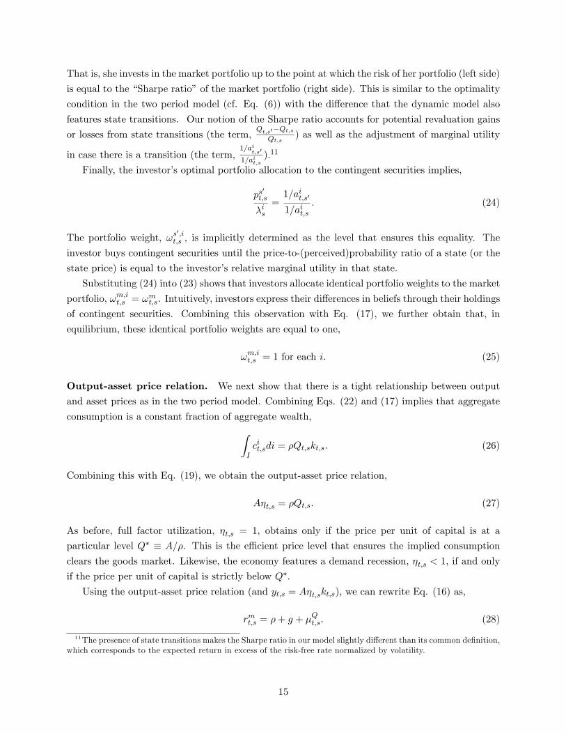
That is, she invests in the market portfolio up to the point at which the risk of her portfolio (left side)

is equal to the “Sharpe ratio”of the market portfolio (right side). This is similar to the optimality

condition in the two period model (cf. Eq. (6)) with the difference that the dynamic model also

features state transitions. Our notion of the Sharpe ratio accounts for potential revaluation gains

or losses from state transitions (the term,Qt,s′−Qt,s

Qt,s) as well as the adjustment of marginal utility

in case there is a transition (the term,1/ai

t,s′

1/ait,s).11

Finally, the investor’s optimal portfolio allocation to the contingent securities implies,

ps′t,s

λis=

1/ait,s′

1/ait,s. (24)

The portfolio weight, ωs′,it,s , is implicitly determined as the level that ensures this equality. The

investor buys contingent securities until the price-to-(perceived)probability ratio of a state (or the

state price) is equal to the investor’s relative marginal utility in that state.

Substituting (24) into (23) shows that investors allocate identical portfolio weights to the market

portfolio, ωm,it,s = ωmt,s. Intuitively, investors express their differences in beliefs through their holdings

of contingent securities. Combining this observation with Eq. (17), we further obtain that, in

equilibrium, these identical portfolio weights are equal to one,

ωm,it,s = 1 for each i. (25)

Output-asset price relation. We next show that there is a tight relationship between output

and asset prices as in the two period model. Combining Eqs. (22) and (17) implies that aggregate

consumption is a constant fraction of aggregate wealth,∫Icit,sdi = ρQt,skt,s. (26)

Combining this with Eq. (19), we obtain the output-asset price relation,

Aηt,s = ρQt,s. (27)

As before, full factor utilization, ηt,s = 1, obtains only if the price per unit of capital is at a

particular level Q∗ ≡ A/ρ. This is the effi cient price level that ensures the implied consumption

clears the goods market. Likewise, the economy features a demand recession, ηt,s < 1, if and only

if the price per unit of capital is strictly below Q∗.

Using the output-asset price relation (and yt,s = Aηt,skt,s), we can rewrite Eq. (16) as,

rmt,s = ρ+ g + µQt,s. (28)

11The presence of state transitions makes the Sharpe ratio in our model slightly different than its common definition,which corresponds to the expected return in excess of the risk-free rate normalized by volatility.

15

In equilibrium, the dividend yield on the market portfolio is equal to the consumption rate ρ.

Combining the output-asset price relation with the interest rate policy in (21), we also summa-

rize the goods market with,

Qt,s ≤ Q∗, rft,s ≥ 0, where at least one condition is an equality. (29)

In particular, the equilibrium at any time and state takes one of two forms. If the natural interest

rate is nonnegative, then the interest rate policy ensures that the price per unit of capital is at

the effi cient level, Qt,s = Q∗, capital is fully utilized, ηt,s = 1, and output is equal to its potential,

yt,s = Akt,s. Otherwise, the interest rate is constrained, rft,s = 0, the price is at a lower level,

Qt,s < Q∗, and output is determined by aggregate demand according to Eq. (27).

For future reference, we also characterize the first-best equilibrium without interest rate rigidi-

ties. In this case, there is no lower bound constraint on the interest rate, so the price per unit of

capital is at its effi cient level at all times and states, Qt,s = Q∗. Combining this with Eq. (28), we

obtain

rmt,s = ρ+ g. (30)

Substituting this into Eq. (23) and using Eq. (25), we solve for “rstar”as,

rf∗s = ρ+ g − σ2s for each s ∈ {1, 2} . (31)

Hence, in the first-best equilibrium the risk premium shocks are fully absorbed by the interest rate.

Next, we characterize the equilibrium with interest rate rigidities.

4. Common beliefs benchmark and amplification

In this section, we analyze the equilibrium in a benchmark case in which all investors share the

same belief. That is, λis ≡ λs for each i. We also normalize the total mass of investors to one so

that individual and aggregate allocations are the same. We use this benchmark to illustrate how

the spirals between asset prices and output exacerbate the recession, and how pessimism amplifies

these spirals.

Because the model is linear, we conjecture that the price and the interest rate will remain

constant within states, Qt,s = Qs and rft,s = rfs (in particular, there is no price drift, µ

Qt,s = 0).

Since the investors are identical, we also have ωmt,s = 1 and ωs′t,s = 0. In particular, the representative

investor’s wealth is equal to aggregate wealth, at,s = Qt,skt,s. Combining this with Eq. (23) and

substituting for rmt,s from Eq. (28), we obtain the following risk balance conditions,

σs =ρ+ g + λs

(1− Qs

Qs′

)− rfs

σsfor each s ∈ {1, 2} . (32)

These equations are the dynamic counterpart to Eq. (7) in the two-period model. They say that,

16

in each state, the total risk in the economy (the left side) is equal to the Sharpe ratio perceived by

the representative investor (the right side). Note that the Sharpe ratio accounts for the fact that

the aggregate wealth (as well as the marginal utility) will change if there is a state transition.12

The equilibrium is then characterized by finding four unknowns,(Q1, r

f1 , Q2, r

f2

), that solve

the two equations (32) together with the two goods market equilibrium conditions (29). We solve

these equations under the following parametric restriction.

Assumption 1. σ22 > ρ+ g > σ21.

In view of this restriction, we conjecture an equilibrium in which the low-risk-premium state 1

features positive interest rates, effi cient asset prices, and full factor utilization, rf1 > 0, Q1 = Q∗ and

η1 = 1, whereas the high-risk-premium state 2 features zero interest rates, lower asset prices, and

imperfect factor utilization, rf2 = 0, Q2 < Q∗ and η2 < 1. In particular, the analysis with common

beliefs reduces to finding two unknowns,(Q2, r

f1

), that solve the two risk balance equations (32)

(after substituting Q1 = Q∗ and rf2 = 0).

Equilibrium in the high-risk-premium state. After substituting rf2 = 0, the risk balance

equation (32) for the high-risk-premium state s = 2 can be written as,

σ2 =ρ+ g + λ2

(1− Q2

Q∗

)σ2

. (33)

In view of Assumption 1, if the price were at its effi cient level, Q2 = Q∗, the risk (the left side)

would exceed the Sharpe ratio (the right side). As in the two period model, the economy generates

too much risk relative to what the investors are willing to absorb at the constrained level of the

interest rate. As before, the price per unit of capital, Q2, needs to decline to equilibrate the risk

markets. Rearranging the expression, we obtain a closed form solution,

Q2 = Q∗(

1− σ22 − (ρ+ g)

λ2

). (34)

As this expression illustrates, we require a minimum degree of optimism to ensure an equilibrium

with positive price and output.

Assumption 2. λ2 > σ22 − (ρ+ g).

This requirement is a manifestation of an amplification mechanism that we describe next.

Amplification from endogenous output and earnings. In the two period model of Section

2, the future payoff from the market portfolio is exogenous (z1). Therefore, a decline in the price

12To see this, observe that the term,Qt,s′−Qt,s

Qt,s′, in the equation is actually equal to, Qt,s

Qt,s′

Qt,s′−Qt,sQt,s

. Here,Qt,s′−Qt,s

Qt,s

denotes the capital gains and Qt,sQt,s′

denotes the marginal utility adjustment when there is a representative investor

(see (23)).

17

of capital (Q) increases the dividend yield and the market return, rm (z1) = z1/Q [cf. Eq. (2)].

In contrast, in the current model the instantaneous payoff from the market portfolio is endogenous

and given by yt,2 = ρQ2kt,2. Therefore, a decline in the price of the market portfolio does not

affect the dividend yield ( yt,2ρQ2kt,2

= ρ) and leaves the market return absent transitions unchanged,

rm = ρ + g [cf. Eq. (28)]. Unlike in the two period model, a decline in asset prices does not

increase the market return any more (aside from state transitions). The intuition is that a lower

price reduces output and economic activity, which reduces firms’earnings and leaves the dividend

yield constant. Thus, asset price declines no longer play a stabilizing role, leaving the economy

susceptible to a spiraling decline.

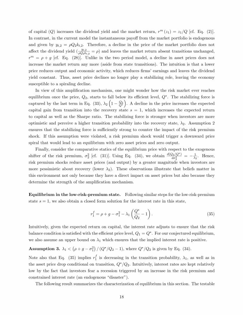
In view of this amplification mechanism, one might wonder how the risk market ever reaches

equilibrium once the price, Q2, starts to fall below its effi cient level, Q∗. The stabilizing force is

captured by the last term in Eq. (33), λ2(

1− Q2Q∗

). A decline in the price increases the expected

capital gain from transition into the recovery state s = 1, which increases the expected return

to capital as well as the Sharpe ratio. The stabilizing force is stronger when investors are more

optimistic and perceive a higher transition probability into the recovery state, λ2. Assumption 2

ensures that the stabilizing force is suffi ciently strong to counter the impact of the risk premium

shock. If this assumption were violated, a risk premium shock would trigger a downward price

spiral that would lead to an equilibrium with zero asset prices and zero output.

Finally, consider the comparative statics of the equilibrium price with respect to the exogenous

shifter of the risk premium, σ22 [cf. (31)]. Using Eq. (34), we obtain d(Q2/Q∗)dσ22

= − 1λ2. Hence,

risk premium shocks reduce asset prices (and output) by a greater magnitude when investors are

more pessimistic about recovery (lower λ2). These observations illustrate that beliefs matter in

this environment not only because they have a direct impact on asset prices but also because they

determine the strength of the amplification mechanism.

Equilibrium in the low-risk-premium state. Following similar steps for the low-risk-premium

state s = 1, we also obtain a closed form solution for the interest rate in this state,

rf1 = ρ+ g − σ21 − λ1(Q∗

Q2− 1

). (35)

Intuitively, given the expected return on capital, the interest rate adjusts to ensure that the risk

balance condition is satisfied with the effi cient price level, Q1 = Q∗. For our conjectured equilibrium,

we also assume an upper bound on λ1 which ensures that the implied interest rate is positive.

Assumption 3. λ1 <(ρ+ g − σ21

)/ (Q∗/Q2 − 1), where Q∗/Q2 is given by Eq. (34).

Note also that Eq. (35) implies rf1 is decreasing in the transition probability, λ1, as well as in

the asset price drop conditional on transition, Q∗/Q2. Intuitively, interest rates are kept relatively

low by the fact that investors fear a recession triggered by an increase in the risk premium and

constrained interest rate (an endogenous “disaster”).

The following result summarizes the characterization of equilibrium in this section. The testable

18

predictions regarding the effect of risk premium shocks on consumption and output follow from

combining the characterization with Eqs. (26) and (27).

Proposition 1. Consider the model with two states, s ∈ {1, 2}, with common beliefs and Assump-tions 1-3. The low-risk-premium state 1 features a positive interest rate, effi cient asset prices and

full factor utilization, rf1 > 0, Q1 = Q∗ and η1 = 1. The high-risk-premium state 2 features zero

interest rate, lower asset prices, and a demand-driven recession, rf2 = 0, Q2 < Q∗, and η2 < 1, as

well as a lower level of consumption and output, ct,2/kt,2 = yt,2/kt,2 = ρQ2. The price in state 2

and the interest rate in state 1 are given by Eqs. (34) and (35).

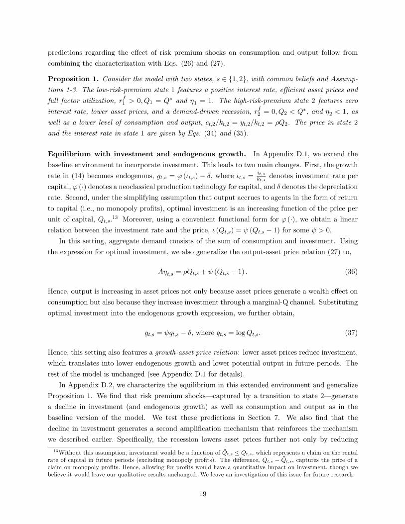
Equilibrium with investment and endogenous growth. In Appendix D.1, we extend the

baseline environment to incorporate investment. This leads to two main changes. First, the growth

rate in (14) becomes endogenous, gt,s = ϕ (ιt,s) − δ, where ιt,s =it,skt,s

denotes investment rate per

capital, ϕ (·) denotes a neoclassical production technology for capital, and δ denotes the depreciationrate. Second, under the simplifying assumption that output accrues to agents in the form of return

to capital (i.e., no monopoly profits), optimal investment is an increasing function of the price per

unit of capital, Qt,s.13 Moreover, using a convenient functional form for ϕ (·), we obtain a linearrelation between the investment rate and the price, ι (Qt,s) = ψ (Qt,s − 1) for some ψ > 0.

In this setting, aggregate demand consists of the sum of consumption and investment. Using

the expression for optimal investment, we also generalize the output-asset price relation (27) to,

Aηt,s = ρQt,s + ψ (Qt,s − 1) . (36)

Hence, output is increasing in asset prices not only because asset prices generate a wealth effect on

consumption but also because they increase investment through a marginal-Q channel. Substituting

optimal investment into the endogenous growth expression, we further obtain,

gt,s = ψqt,s − δ, where qt,s = logQt,s. (37)

Hence, this setting also features a growth-asset price relation: lower asset prices reduce investment,

which translates into lower endogenous growth and lower potential output in future periods. The

rest of the model is unchanged (see Appendix D.1 for details).

In Appendix D.2, we characterize the equilibrium in this extended environment and generalize

Proposition 1. We find that risk premium shocks– captured by a transition to state 2– generate

a decline in investment (and endogenous growth) as well as consumption and output as in the

baseline version of the model. We test these predictions in Section 7. We also find that the

decline in investment generates a second amplification mechanism that reinforces the mechanism

we described earlier. Specifically, the recession lowers asset prices further not only by reducing

13Without this assumption, investment would be a function of Qt,s ≤ Qt,s, which represents a claim on the rentalrate of capital in future periods (excluding monopoly profits). The difference, Qt,s − Qt,s, captures the price of aclaim on monopoly profits. Hence, allowing for profits would have a quantitative impact on investment, though webelieve it would leave our qualitative results unchanged. We leave an investigation of this issue for future research.

19

output and earnings but also by reducing investment and growth (in potential output and earnings).

Figure 1 in the introduction presents a graphical illustration of the two amplification mechanisms.

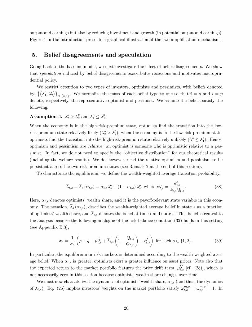
5. Belief disagreements and speculation

Going back to the baseline model, we next investigate the effect of belief disagreements. We show

that speculation induced by belief disagreements exacerbates recessions and motivates macropru-

dential policy.

We restrict attention to two types of investors, optimists and pessimists, with beliefs denoted

by,{(λi1, λ

i2

)}i∈{o,p}. We normalize the mass of each belief type to one so that i = o and i = p

denote, respectively, the representative optimist and pessimist. We assume the beliefs satisfy the

following:

Assumption 4. λo2 > λp2 and λo1 ≤ λ

p1.

When the economy is in the high-risk-premium state, optimists find the transition into the low-

risk-premium state relatively likely (λo2 > λp2); when the economy is in the low-risk-premium state,

optimists find the transition into the high-risk-premium state relatively unlikely (λo1 ≤ λp1). Hence,

optimism and pessimism are relative: an optimist is someone who is optimistic relative to a pes-

simist. In fact, we do not need to specify the “objective distribution” for our theoretical results

(including the welfare results). We do, however, need the relative optimism and pessimism to be

persistent across the two risk premium states (see Remark 2 at the end of this section).

To characterize the equilibrium, we define the wealth-weighted average transition probability,

λt,s ≡ λs (αt,s) ≡ αt,sλos + (1− αt,s)λps, where αot,s =aot,s

kt,sQt,s. (38)

Here, αt,s denotes optimists’wealth share, and it is the payoff-relevant state variable in this econ-

omy. The notation, λs (αt,s), describes the wealth-weighted average belief in state s as a function

of optimists’wealth share, and λt,s denotes the belief at time t and state s. This belief is central to

the analysis because the following analogue of the risk balance condition (32) holds in this setting

(see Appendix B.3),

σs =1

σs

(ρ+ g + µQt,s + λt,s

(1− Qt,s

Qt,s′

)− rft,s

)for each s ∈ {1, 2} . (39)

In particular, the equilibrium in risk markets is determined according to the wealth-weighted aver-

age belief. When αt,s is greater, optimists exert a greater influence on asset prices. Note also that

the expected return to the market portfolio features the price drift term, µQt,s [cf. (28)], which is

not necessarily zero in this section because optimists’wealth share changes over time.

We must now characterize the dynamics of optimists’wealth share, αt,s (and thus, the dynamics

of λt,s). Eq. (25) implies investors’weights on the market portfolio satisfy ωm,ot,s = ωm,pt,s = 1. In

20

0 5 10 15 20 25 300.05

0.10

0 5 10 15 20 25 30

0.1

0.15

0.2

0.25

0.3

0.35

0.4

0.45

0.5

Figure 2: A simulation of the dynamics of optimists’wealth share over time.

Appendix B.3, we also solve for investors’weights on the contingent securities,

ωs′,ot,s = λos − λt,s = (λos − λps) (1− αt,s) . (40)

Thus, investors settle their disagreements on the jump risk by trading the contingent securities.

Optimists take a positive position on a contingent security whenever their belief for the transi-

tion probability exceeds the weighted average belief. This implies that their wealth share evolves

according to [cf. Eqs. (B.13) and (B.14)],{αt,s = (λps − λos)αt,s (1− αt,s) , if there is no state change,

αt,s′/αt,s = λos/λt,s, if there is a state change to s′.(41)

Here, αt,s =dαt,sdt denotes the derivative with respect to time. As long as the economy remains in

the boom state, optimists’wealth share drifts upwards (since λo1 < λp1), because they make profits

from selling insurance– contingent contracts that pay in the recession state. If there is a jump to

the recession state, optimists’wealth share makes a downward jump. Conversely, optimists’wealth

share drifts downwards in the recession state, and it makes an upward jump if there is a transition

to the boom state. Figure 2 illustrates the dynamics of optimists’wealth share for a particular

parameterization (described subsequently) and realization of uncertainty.

These observations also imply that the weighted average belief in (38) (that determines asset

prices) is effectively extrapolative in the sense that good realizations increase effective optimism

whereas bad realizations reduce it. Specifically, as the boom state persists, optimists’wealth share

increases and the aggregate belief becomes more optimistic. After a transition to the recession state,

the aggregate belief becomes less optimistic. Similarly, the aggregate belief becomes less optimistic

21

as the recession persists, and it becomes more optimistic after a transition into the boom.

Eq. (41) determines the evolution of optimists’wealth share (and thus, the weighted average

belief) regardless of the level of asset prices and output. The equilibrium is determined by jointly

solving this expression together with the risk balance condition (39) and the goods market equi-

librium condition (29). To make progress, we suppose Assumptions 1-3 from the previous section

hold according to both belief types. This ensures that, regardless of the wealth shares, the low-

risk-premium state 1 features a positive interest rate, effi cient price level, and full factor utilization,

rft,1 > 0, Qt,1 = Q∗, ηt,1 = 1, and the high-risk-premium state 2 features a zero interest rate, a lower

price level, and insuffi cient factor utilization, rft,2 = 0, Qt,2 < Q∗, ηt,2 < 1. We next characterize

this equilibrium starting with the high-risk-premium state. In this as well as the next section, we

also find it convenient to work with the log of the price level, qt,s ≡ logQt,s.

Equilibrium in the high-risk-premium state. Consider the risk balance equation (39) for

state s = 2. Using µQt,2 =dQt,2/dtQt,2

= qt,2, we obtain the following analogue of Eq. (33),

σ2 =1

σ2

(ρ+ g + qt,2 + λt,2

(1− Q2

Q∗

)). (42)

Combining this with Eq. (41), we obtain a differential equation system that describes the joint

dynamics of the log price and optimists’wealth share, (qt,2, αt,2), conditional on no transition.

In Appendix B.3, we show that this system is saddle path stable: for any initial wealth share,

αt,2 ∈ (0, 1), there exists a unique equilibrium price level, qt,2 ∈ [qp2 , qo2), such that the solution

satisfies limt→∞ αt,2 = 0 and limt→∞ qt,2 = qp2 . Here, qi2 denotes the log price level with common

beliefs characterized in Section 4 corresponding to type i investors’ belief. The system is also

stationary, which implies that the price can be written as a function of optimists’wealth share.

The price function, q2 (α), is characterized as the solution to the following differential equation in

α-domain,

q′2 (α) (λo2 − λp2)α (1− α) = ρ+ g + λ2 (α)

(1− exp (q2 (α))

Q∗

)− σ22, (43)

with boundary conditions, q2 (0) = qp2 and q2 (1) = qo2. We further show that q2 (α) is strictly

increasing in α. As in the previous section, greater optimism increases the asset price in the

high-risk-premium state.14

Equilibrium in the low-risk-premium state. Following similar steps for the risk balance

condition for the low-risk-premium state s = 1, we obtain,

rf1 (α) = ρ+ g − λ1 (α)

(Q∗

exp (q2 (α′))− 1

)− σ21 where α′ =

αλo1λ1 (α)

. (44)

14 Introducing partial nominal price flexibility along the lines discussed in Remark 1 would create a second channelby which increasing optimists’wealth share would increase real asset prices. In that environment, pessimists wouldperceive lower expected inflation than optimists (because they believe the economy is more likely to stay in recession),which would lead to a greater perceived real interest rate and lower real asset valuations.

22

0 0.1 0.2 0.3 0.4 0.5 0.6 0.7 0.8 0.9 10.9

0.91

0.92

0.93

0.94

0.95

0.96

0 0.1 0.2 0.3 0.4 0.5 0.6 0.7 0.8 0.9 1

0.005

0.01

0.015

0.02

0.025

0.03

0.035

Figure 3: Equilibrium price and interest rate functions with heterogeneous beliefs.

Here, rf1 (α) denotes the interest rate when optimists’wealth share is equal to α. The term, α′,

denotes optimists’wealth share after an immediate transition into the high-risk-premium state [cf.

Eq. (41)]. The interest rate depends on (among other things) the weighted average transition

probability into the high-risk-premium state, λ1 (α), as well as the price level that would obtain

after transition, q2 (α′). It is easy to check that rf1 (α) is increasing in α, since, as in the previous

section, greater optimism increases asset prices.

The following proposition summarizes the characterization of equilibrium. The last part, which

follows by combining the characterization with Eqs. (26) and (27), shows that greater optimists’

wealth share in the high-risk-premium state mitigates the severity of the recession.

Proposition 2. Consider the model with two belief types. Suppose Assumptions 1-3 hold for eachbelief, and that beliefs are ranked according to Assumption 4. Then, optimists’wealth share evolves

according to Eq. (41). The equilibrium log-price and interest rate can be written as a function of

optimists’ wealth share, q1 (α) , rf1 (α) , q2 (α) , rf2 (α). In the low-risk-premium state, q1 (α) = q∗,

and rf1 (α) is an increasing function of α given by Eq. (44). In the high-risk-premium state, rf2 (α) =

0, and q2 (α) is an increasing function of α that solves the differential equation (43) with q2 (0) = qp2and q2 (1) = qo2. Greater optimists’wealth share in the high-risk-premium state, αt,2, increases the

price per capital, Qt,2, as well as consumption and output, ct,2/kt,2 = yt,2/kt,2 = ρQt,2.

Numerical illustration. We next illustrate the equilibrium using a simple parameterization (see

Appendix B.4 for details). For the baseline parameters, we set g = 5%, ρ = 4%, σ21 = 5%, σ22 = 10%.

For investors’beliefs about transition probabilities, we set λo1 = 1/10, λp1 = 1/3 for the boom state

and λo2 = 1/3, λp2 = 1/10 for the recession state.

Figure 3 illustrates the corresponding equilibrium. The left panel illustrates the price of capital

in the recession (normalized by the effi cient price level) as a function of optimists’wealth share.

When pessimists dominate the economy, the price of capital and output decline by 10%. In contrast,

23

0 5 10 15 20 25 300.05

0.10

0 5 10 15 20 25 30

0

0.02

0.04

0 5 10 15 20 25 30

0.92

0.94

0.96

0.98

1

0 5 10 15 20 25 30

0.92

0.94

0.96

0.98

1

Figure 4: A simulation of the equilibrium variables over time with belief disagreements (solid redline), with common beliefs (dashed red line), and the first-best benchmark (circled blue line).

when optimists dominate, they decline by only 3%. The right panel of Figure 3 illustrates the

interest rate in the boom as a function of optimists’wealth share. The risk-free rate during the

boom is close to 4% when optimists dominate the economy but it is close to 0% when pessimists

dominate.

Amplification from speculation. We next use our numerical example to illustrate how spec-

ulation further amplifies the business-cycle driven by risk premium shocks. To this end, we fix

investors’beliefs and simulate the equilibrium for a particular realization of uncertainty over a 30-

year horizon. We choose the (objective) simulation belief to be in the “middle”of optimists’and

pessimists’beliefs in terms of the relative entropy distance.15 Figure 4 illustrates the dynamics of

equilibrium variables (except for optimists’wealth share, which we plot in Figure 2). For compari-

15This ensures that there is a non-degenerate long-run wealth distribution in which neither optimists nor pessimistspermanently dominate, which helps to visualize the destabilizing effects of speculation without taking a stand onwhether optimists and pessimists are “correct.”Our welfare results in the next section do not require this assumptionsince we evaluate investors’expected utilities according to their own beliefs.

24

son, the dashed red line plots the equilibrium that would obtain in the common-beliefs benchmark

if all investors shared the “middle” simulation belief, and the circled blue line plots the first-best

equilibrium that would obtain without interest rate rigidities.

The figure illustrates two points. First, consistent with our baseline analysis in the previous

section, the price per unit of capital is more volatile and the interest rate is more compressed

than in the first-best equilibrium. In the high-risk-premium state, the interest rate cannot decline

suffi ciently to equilibrate the risk balance condition, which leads to a drop in asset prices and

a demand recession. In the low-risk-premium state, the fear of transition into the recessionary

high-risk-premium state keeps the interest rate lower than in the first-best benchmark.

Second, risk-centric recessions are more severe when investors have belief disagreements (and

this also leads to more compressed interest rates). The intuition follows from Figures 2 and 3.

Speculation in the low-risk-premium state decreases optimists’ wealth share once the economy

transitions into the high-risk-premium state, as illustrated by Figure 2, which translates into lower

asset prices and a more severe demand recession, as illustrated by Figure 3 and Proposition 2.

Speculation also increases optimists’wealth share if the boom continues, but this effect does not

translate into higher asset prices or output since it is (optimally) neutralized by the interest rate

response. The adverse effects of speculation on demand recessions motivates the analysis of macro-

prudential policy, which we analyze in the next section.

Remark 2 (Interpretation of Belief Disagreements). As this discussion suggests, what matters forour results on speculation is persistent heterogeneous valuations for risky assets that ensure: (i)

during the boom, high-valuation investors absorb relatively more of the recession risks, and (ii) dur-

ing the recession, greater wealth share of high-valuation investors increases the (relative) price of

risky assets. Belief disagreements generate these features naturally, under the mild assumption that

optimists and pessimists do not flip roles across booms and recessions,16 but other sources of hetero-

geneous valuations would lead to similar results. For example, with heterogeneity in risk aversion,

more risk tolerant agents take on more aggregate risk (i.e., they insure less risk tolerant agents),

which reduces their wealth share and the (relative) price of risky assets following negative shocks

to fundamentals (see, for instance, Garleanu and Pedersen (2011); Longstaff and Wang (2012)).

From this perspective, belief disagreements can also capture institutional reasons for heterogeneous

valuations such as capacity or mandates for handling risk. Investment banks, for example, have far

larger capacity to handle and lever risky positions than pensioners and money market funds.

Formally, given two probability distributions (p (s))s∈S and (q (s))s∈S , relative entropy of p with respect to q is

defined as∑s p (s) log

(p(s)q(s)

). Blume and Easley (2006) show that, in a setting with independent and identically

distributed shocks (and identical discount factors), only investors whose beliefs have the maximal relative entropydistance to the true distribution survive. Since our setting features Markov shocks, we apply their result state-by-stateto pick the simulation belief that ensures conditional transition probabilities satisfy the necessary survival conditionfor optimists as well as pessimists.16This assumption is supported by recent survey evidence that shows belief heterogeneity is largely explained

by persistent individual heterogeneity (Giglio et al. (2019)). The assumption is also consistent with an extensivepsychology literature that documents the prevalence of optimism, as well as its heterogeneity and persistence, sinceit is largely a personal trait (see Carver et al. (2010) for a review).

25

6. Welfare analysis and macroprudential policy

Since our model features constrained monetary policy, most of the aggregate demand boosting

policies that have been discussed in the New Keynesian literature are also effective in our envi-

ronment. We skip a discussion of these policies for brevity (our results would still apply as long

as these policies are imperfect). Instead, we focus on macroprudential policy interventions that

impose restrictions on risk market participants with the objective of obtaining macroeconomic ben-

efits. In practice, most macroprudential policies restrict risk taking by banks– especially large

ones. Interpreting banks as relatively high-valuation investors (see Remark 2) or as lenders to such

investors (see Section 7), we capture these policies in reduced form by imposing portfolio risk limits

on relatively optimistic investors.

Our model features heterogeneous beliefs, which makes the welfare analysis challenging. We

adopt the standard Pareto criterion in which the planner evaluates investors’ expected utility

according to their own beliefs. We adopt the standard criterion to highlight that our results

are not driven by paternalistic concerns. Rather, the planner improves welfare by internalizing

aggregate demand externalities. The standard criterion is also appropriate if we interpret belief

disagreements as a modeling device to capture heterogeneous valuations due to other factors (see

Remark 2). However, if we interpret belief disagreements literally, then a paternalistic criterion

such as the belief-neutral welfare criterion developed by Brunnermeier et al. (2014) could be more

appropriate. Adopting this belief-neutral criterion would reinforce our normative conclusions: in

that case, macroprudential policy would not only improve macroeconomic outcomes but it would

also mitigate the microeconomic costs associated with speculation (see, e.g., Simsek (2013b); Dávila

(2017); Heimer and Simsek (2019)).

Using the standard welfare criterion also helps to simplify the theoretical analysis. Since our

model features complete markets and no frictions other than interest rate rigidities, aggregate

demand externalities constitute the only source of ineffi ciency. Therefore, the first-best benchmark

that also corrects for these ineffi ciencies is Pareto effi cient. This enables us to isolate the aggregate

demand externalities by defining investors’gap values: the difference between their expected value

in equilibrium relative to the expected value in the first-best benchmark. The gap value captures

the present discounted value of the investor’s utility losses due to demand recessions. Focusing

on the gap value simplifies the analysis considerably because, up to a first order, macroprudential

policies affect social welfare only through their impact on investors’gap values (in view of the fact

that the first-best benchmark is Pareto effi cient).

The formal analysis in this section proceeds as follows. Using the model with two belief types

from the previous section, we first characterize investors’ value functions in equilibrium accord-

ing to their own beliefs. We define the gap value functions and illustrate the aggregate demand

externalities. We then show that macroprudential policy that induces optimists to act more pes-

simistically (via appropriate portfolio risk limits), but that otherwise does not distort allocations,

can generate a Pareto improvement of social welfare. We focus on macroprudential policy in the

boom (low-risk-premium) state and provide a brief discussion of the macroprudential policy in the

26

recession (high-risk-premium) state.

Value function in equilibrium. Because the model is linear, investors’expected utility can be

written as (see Appendix B.1.1),

V it,s

(ait,s)

=log(ait,s/Qt,s

)ρ

+ vit,s. (45)

Here, vit,s denotes the normalized value function per unit of capital stock. In Appendix C.1, we

further characterize it as the solution to the following differential equation system,

ρvit,s −∂vit,s∂t

= log ρ+ qt,s +1

ρ

g − 12σ

2s

−(λis − λt,s

)+ λis log

(λisλt,s

) + λis(vit,s′ − vit,s

). (46)

The equilibrium price, qt,s, affects investors’welfare since it determines output and consumption

[cf. Eqs. (26) and (27)]. Consumption growth, g, and volatility, σ2s, also affect welfare. Finally,

speculation affects investors’ (perceived) welfare. This is captured by the term, −(λis − λt,s

)+

λis log(λisλt,s

), which is zero with common beliefs, and strictly positive with disagreements.

Gap value function. To facilitate the policy analysis, we break down the value function into

two components,

vit,s = vi,∗t,s + wit,s. (47)

Here, vi,∗t,s denotes the first-best value function that would obtain if there were no interest rate

rigidities. It is characterized by solving Eq. (46) with the effi cient price level, qt,s = q∗, for each

t, s. The residual, wit,s = vit,s− vi,∗t,s , denotes the gap value function, which captures the loss of value

due to interest rate rigidities and demand recessions. As we will see below, the first-order impact of

macroprudential policy on social welfare depends only on the gap value function. Using Eq. (46),

we characterize the gap value function as the solution to the following system,

ρwit,s = qt,s − q∗ +∂wit,s∂t

+ λis(wit,s′ − wit,s

). (48)

This illustrates that, in view of the output-asset price relation (27), the gap value function depends

on the asset prices relative to the effi cient level. Recall also that the equilibrium features qt,1 = q∗

and qt,2 < q∗. Thus, the key objective of policy interventions in this environment is to increase the

asset price in the high-risk-premium state (so as to mitigate the demand recession).

Aggregate demand externalities. In Appendix C.1, we show that the gap value function can

be written as a function of optimists’wealth share, wis (α). Combining Eqs. (48) and (41), we also

27

characterize this function as the solution to the following system in α-domain,

ρwis (α) = qs (α)− q∗ − (λos − λps)α (1− α)∂wis (α)

∂α+ λis

(wis′(α′)− wis (α)

), (49)

where α′ = αλos/λs (α). Recall that the price function in the high-risk-premium state, q2 (α), is

increasing in optimists’wealth share [cf. Figure 3]. This leads to the following result.

Lemma 1. The gap value function satisfies, dwis(α)dα > 0 for each s, i and α ∈ (0, 1).

Intuitively, optimists’wealth share is a scarce resource that brings asset prices and output in the

high-risk-premium state closer to its first-best level. Thus, the gap value function in the high-risk-

premium state is increasing in optimists’wealth share. The gap value function in the other state

is also increasing, because the economy can always transition into the high-risk-premium state,

where optimists’wealth share is useful (see Lemma 2 below for a ranking of the marginal value of

optimists’wealth share across the two states).

The result also illustrates the aggregate demand externalities. Optimists’wealth share is an

endogenous variable that fluctuates due to investors’portfolio decisions [cf. Figure 2]. Individual

optimists that take positions in contingent markets– and pessimists that take the other side of

these positions– do not take into account the impact of their decisions on asset prices and social

welfare. This leads to ineffi ciencies that can be corrected by macroprudential policy.

Equilibrium and gap value functions with macroprudential policy. To evaluate the di-

rection of the ineffi ciency, we consider a constrained policy exercise where the planner can induce

optimists to choose allocations as if they have less optimistic beliefs.17 Specifically, optimists are

constrained to choose allocations as-if they have the beliefs, λo,pl ≡(λo,pl1 , λo,pl2

), that satisfy,

λo,pl1 ≥ λo1 and λo,pl2 ≤ λo2. Pessimists continue to choose allocations according to their own beliefs.

Throughout, we use λi,pls to denote investors’ as-if beliefs and λis to denote their actual beliefs

(for pessimists, the two beliefs coincide). We also use λpls (α) = αλo,pls + (1− α)λps to denote the

weighted average as-if belief.

In Appendix C.2, we show that the planner can implement this policy by imposing inequality re-

strictions on optimists’portfolio weights, while allowing them to make unconstrained consumption-

savings decisions. Specifically, when the risk premium is low, the policy constrains optimists from

taking too negative a position on the contingent security that pays if there is a transition to the

high-risk-premium state, ω2,ot,1 ≥ ω2,ot,1 (restrictions on selling “put options”). When the risk premium

is high, the policy constrains optimists from taking too large a position on the contingent security

that pays if there is a transition to the low-risk-premium state, ω1,ot,2 ≤ ω1,ot,2 (restrictions on buying

“call options”). Finally, in either state, the policy also constrains optimists’weight on the market

portfolio not to exceed the market average, ωm,ot,s ≤ 1 (since otherwise optimists start to speculate

by increasing their exposure to the market portfolio).17For simplicity, we restrict attention to time-invariant policies. The planner commits to a policy at time zero,(λo,pl1 , λo,pl2

), and implements it throughout.

28

The characterization of equilibrium with policy is then the same as in Section 5. In particular,

Eqs. (41) and (42) still hold with the only difference that investors’beliefs are replaced with their

as-if beliefs, λi,pls . We denote the resulting price functions with qpls (α) to emphasize that they are

determined by as-if beliefs (as opposed to actual beliefs). On the other hand, the equation system

that characterizes the gap value function is given by,

ρwis (α) = qpls (α)− q∗ −(λo,pls − λps

)α (1− α)

∂wis (α)

∂α+ λis

(wis′(α′,pl

)− wis (α)

)(50)

where α′,pl = αλo,pls /λo,pls (α). Comparing this with Eq. (49) illustrates that the macroprudential

policy can affect the gap value through two potential channels. First, it might affect the equilibrium

asset prices (captured by the term, qpls (α)). Second, the policy affects the dynamics of optimists’

wealth share, which in turn influence the gap value. For example, in the low-risk-premium state

s = 1, the policy increases λo,pl1 , which induces optimists to increase their position on the contingent

security that pays if there is a transition into the high-risk-premium state [cf. Eq. (40)]. This

increases optimists’wealth share after a transition (captured by the term, α′,pl) at the expense of

reducing optimists’wealth share in case there is no transition (captured by the term, −(λo,pls − λps

)).

Planner’s Pareto problem. To trace the Pareto frontier, we allow the planner to make a one-

time wealth transfer among the investors at time zero. In Appendix C.2, we show that the planner’s

Pareto problem can then be reduced to,

maxλo,pl

vpl0,s = α0,svo0,s + (1− α0,s) vp0,s. (51)

Hence, the planner maximizes a wealth-weighted average of investors’normalized values (where the

wealth shares correspond to Pareto weights). We also decompose the planner’s value function into

first-best and gap value components, vpl0,s = vpl,∗0,s + wpl0,s.

A key observation is that, since the first-best benchmark does not feature any frictions, it

satisfies the First Welfare Theorem and therefore it is Pareto effi cient. This in turn implies that the

marginal impact of the policy on the planner’s first-best value function is zero,∂vpl,∗0,s

∂λo,pl

∣∣∣∣λo,pl=λo

= 0.

18 Consequently, the first order impact of the policy is characterized by its impact on the planner’s

gap value function,

wpl0,s = α0,swo0,s + (1− α0,s)wp0,s. (52)

Macroprudential policy in the low-risk-premium state. Now suppose the economy is in

the low-risk-premium state s = 1. The planner can use macroprudential policy in the current state,

λo,pl1 ≥ λo1 (she can induce optimists to act as if transition into the recession is more likely), but

not in the other state λo,pl2 = λo2 (she cannot influence optimists’actions in the recession state).

18 If this wasn’t the case, the first-best allocations could be Pareto improved by appropriately changing optimists’as-if beliefs.

29

Effectively, this policy induces optimists to sell less of the contingent security that pays in case

there is a transition to the high-risk-premium state, while also preventing optimists from increasing

their position in the market portfolio.

For small changes, this policy does not affect the price function in the current state, qpl1 (α) = q∗

(since we assume beliefs in the boom state are suffi ciently optimistic that the interest rate is not

constrained– see Assumption 3). Hence, the policy affects the gap value only through its impact on

optimists’wealth dynamics and the associated aggregate demand externalities. Differentiating Eq.

(50) (for s = 1) with respect to optimists’as-if beliefs and evaluating at the no-policy benchmark

(λo,pl1 = λo1), we obtain,

(ρ+ λi1

) ∂wi1 (α)

∂λo,pl1

= α (1− α)

[−∂w

i1 (α)

∂α+

λi1λ1 (α)

λp1λ1 (α)

∂wi2 (α′)

∂α

]+ λi1

∂wi2 (α)

∂λo,pl1

, (53)

where α′ = αλo1/λ1 (α). Here, the two terms inside the brackets capture the direct impact of the

policy on welfare through aggregate demand externalities. The second term illustrates that the

policy generates positive aggregate demand externalities– because it increases optimists’wealth

share if there is a transition into the high-risk-premium state. On the other hand, the first term

illustrates that the policy also generates negative aggregate demand externalities– because it re-

duces optimists’wealth share in case there is no transition. Eq. (53) describes the balance of these

externalities when optimists are required to purchase the contingent security at equilibrium prices.

This illustrates that, in a dynamic setting, macroprudential policy in the low-risk-premium state

is associated with some costs as well as benefits. The costs emerge from the fact that the policy

prevents optimists from accumulating wealth that could be useful in a future recession. However,

intuition suggests the benefits should outweigh the costs as long as future recessions are not too

different from an imminent recession. The following lemma verifies this for the special case, λo1 = λp1.

Lemma 2. When λo1 = λp1, the gap value function satisfiesdwi2(α

′)dα >

dwi1(α)dα for each i and α ∈ (0, 1).

That is, optimists’ wealth share increases the gap value more when there is an immediate

transition into the high-risk-premium state, in which case the benefits appear immediately. Any

delay in such transition reduces the benefits by postponing them. Combining this lemma with Eq.

(53) provides a heuristic derivation of our main result in this section (see Appendix C.2 for the

proof).

Proposition 3. Consider the model with two belief types that satisfy λo1 = λp1. Consider the

macroprudential policy in the boom state, λo,pl1 ≥ λo1 (and suppose λo,pl2 = λo2). The policy increases

the planner’s gap value (and thus, also the total value),

∂vpl1 (α)

∂λo,pl1

∣∣∣∣∣λo,pl1 =λo1

=∂wpl1 (α)

∂λo,pl1

∣∣∣∣∣λo,pl1 =λo1

> 0 for each α ∈ (0, 1) .

In particular, regardless of the planner’s Pareto weight, there exists a Pareto improving macropru-

dential policy.

30

What happens when we relax the assumption, λo1 = λp1? This is largely a technical assumption.

We conjecture that Proposition 3 also holds when λo1 < λp1 (under appropriate technical assump-

tions) but we are unable to provide a proof. There are two distinct challenges. First, we cannot

generalize Lemma 2, although the ranking is intuitive and should hold unless there are strong non-

linearities in the gap value function.19 Second, in the more general case pessimists and optimists

disagree about the benefits of macroprudential policy (captured by λi1 in the bracketed terms of

(53)). The planner takes a weighted average of these perceptions, which complicates the analysis.20

Figure 5 illustrates the result for our earlier parameterization (that features λo1 < λp1). We fix

the optimists’wealth share at a particular level (α = 12) and calculate the effect of macroprudential

policy on the planner’s value function as well as on its components. The policy reduces the plan-

ner’s first-best value function, since it distorts investors’allocations according to their own beliefs.

However, for small policy changes, the magnitude of this decline is small (due to the First Wel-

fare Theorem). The policy also generates a relatively sizeable increase in the planner’s gap value

function. This increase is suffi ciently large that the policy increases the actual value function and

generates a Pareto improvement. As the policy becomes larger, the gap value continues to increase

whereas the first-best value decreases. Moreover, the decline in the first-best value is negligible for

small policy changes but it becomes sizeable for large policy changes. The (constrained) optimal

macroprudential policy obtains at an intermediate level.

The result is reminiscent of the analysis in Korinek and Simsek (2016), in which macroprudential

policy improves outcomes by increasing the wealth of high marginal propensity to consume (MPC)

households when there is a demand-driven recession. While both results are driven by aggregate

demand externalities, the mechanism here is different and operates via asset prices. In fact, in our

setting, all investors have the same MPC equal to ρ. Optimists improve aggregate demand in the

high-risk-premium state not because they spend more than pessimists, but because they increase

asset prices and induce all investors to spend more.

Macroprudential policy in the high-risk-premium state. The analysis so far concerns

macroprudential policy in the low-risk-premium state and maintains the assumption that λo,pl2 = λo2.

In Appendix C.2, we also analyze the polar opposite case when the economy is in the high-risk-

premium state s = 2, and the planner can apply macroprudential policy in this state, λo,pl2 ≤ λo2 (she19Specifically, the proof of Lemma 2 establishes,

∂wi1 (b0,1)

∂b=

λi1λi1 + ρ

∫ ∞0

e−(ρ+λi1)t(ρ+ λi1

) ∂wi2 (bt,2)

∂bdt,

where b0,1 denotes a transformed version of α at the initial state, and bt,2 denotes the same variable after a transitioninto the high-risk-premium state after a period of length t. When λo1 = λp1, we also have bt,2 = b0,1 (since there is

no speculation in the low-risk state), which yields∂wi1(b0,1)

∂b=

λi1λi1+ρ

∂wi2(b0,1)∂b

<∂wi2(b0,1)

∂b. When λo1 < λp1, the same

result holds and the ranking remains unchanged if the value function is linear in the transformed variable b. Hence,the ranking can fail only if there are suffi ciently large nonlinearities in the gap value function.20When λo1 = λp1, we actually have the stronger result that

∂wi1(α)

∂λo,pl1

> 0 for each i, that is, the policy increases

the gap value according to optimists and pessimists (see Eq. (C.18)). We state the weaker version of the result inProposition 3 because the stronger version might conceivably fail according to optimists (e.g., if λo1 is close to zero).

31

0.1 0.1002 0.1004 0.1006 0.1008 0.101 0.1012 0.1014 0.1016 0.1018 0.102

­1.5

­1

­0.5

0

0.5

1

1.5

10 ­3

Figure 5: Effect of macroprudential policy in the low-risk-premium state on the planner’s valuefunction and its components.

can induce optimists to act as if the recovery is less likely), but not in the other state, λo,pl1 = λo1.

Proposition 4 in the appendix shows that, in contrast to Proposition 3, this policy can reduce social

welfare. Consider the two counteracting forces. First, similar to before, macroprudential policy

increases the gap value by increasing optimists’wealth share if the economy stays at the high-risk-

premium state. However, unlike before, macroprudential policy also reduces current asset prices

because the price is below the first-best level, qpl2 (α) < q∗, and it is increasing in optimists’as-if

optimism, λo,pl2 (see Eq. (34)). This channel reduces the gap value (see Eq. (50)). When optimists’

wealth share is large (α → 1), the latter channel is dominant and macroprudential policy reduces

the gap value and the social welfare. Even when the latter channel does not dominate, it suggests

that the macroprudential policy in the recession state is less useful than in the boom state (which

we verify in numerical simulations).

It is useful to emphasize that macroprudential policy in the low-risk-premium state does not

lower asset prices due to the monetary policy response. Specifically, while the asset price in this

state is not influenced by policy, qpl1 (α) = q∗, the interest rate, rf1 (α), is decreasing in optimists’

as-if pessimism, λo,pl1 (see Eq. (35)). Intuitively, as macroprudential policy reduces the demand

for risky assets, monetary policy lowers the interest rate to dampen its effect on asset prices and

aggregate demand.

Taken together, our analysis provides support for procyclical macroprudential policy. In states

where output is not demand constrained (in our model, the boom state s = 1), macroprudential

policy that restricts high-valuation investors’ (in our model optimists’) risk taking is desirable.

This policy improves welfare by ensuring that high-valuation investors bring more wealth to the

demand-constrained states, which increases asset prices and output. In states where output is

32

demand constrained (in our model, the recession state s = 2), macroprudential policy is less useful

because it has an immediate negative impact on asset prices and aggregate demand.

7. Empirical evidence

Our empirical analysis focuses on three predictions. First, our model predicts that risk premium

shocks generate an interest rate reduction when the interest rate is not constrained, and a more

severe demand recession when the interest rate is constrained. Second, the recession reduces firms’

earnings and leads to a further reduction in asset prices. Third, the recession is more severe when

the shock takes place in an environment with more speculation. To investigate these predictions, we

compare the response to house price shocks in Eurozone countries (which have constrained interest

rates with respect to national shocks) to the response in non-Eurozone developed countries (which

have less constrained interest rates). At the end of the section, we discuss empirical evidence from

the recent literature which suggests that similar results apply for price shocks to other asset classes,

such as stocks, as well as for other constraints on the interest rate, such as the zero lower bound.

While our model relies on the zero lower bound constraint, the mechanisms are more general,

and we find it more convenient to work with the currency-union constraint in our empirical analysis.

The zero lower bound has only recently become a practical constraint, generating data limitations,

and it calls for an asymmetric specification that requires separate responses to positive and negative

price shocks (since the monetary policy can raise the interest rate in response to positive shocks,

especially if the economy is close to full capacity utilization). In contrast, individual Eurozone

countries have had constrained interest rates (with respect to national shocks) for much longer,

and the constraint has been symmetric with respect to the direction of shocks.

A major challenge in this exercise is the identification of the risk premium shock that drives

asset prices. As we clarify in Section 2, the exact source of the shock is not important for our

mechanisms (e.g., risk, risk aversion, or beliefs have similar effects). Therefore, our strategy is to

control for factors that do not act as a risk premium shock according to our model. In particular,

we attempt to control for supply shocks and demand shocks that are not specific to house prices–

including monetary policy shocks, and we interpret the residual change in house prices as a plausibly

exogenous risk premium shock. Specifically, our risk premium shock is a surprise change in house

prices in a country after controlling for contemporaneous and recent changes in output and the

policy interest rate (as well as the average house price change in sample countries).21

Our model has a single type of capital, which can be interpreted as a value-weighted average

of housing, stocks, and other assets. We focus on house prices for two reasons. First, housing

wealth is large and its size (relative to output) is comparable between Eurozone and non-Eurozone

developed countries (see Table 3 in Appendix E). In contrast, stock markets in Eurozone countries21While our controls are imperfect, we also report the differential effects of these shocks in Eurozone countries

compared to their effects outside the Eurozone, which provides additional robustness. For example, our modelillustrates that permanent supply shocks (e.g., an increase in A) shift asset prices and output regardless of whetherthe interest rate is constrained (see Sections 3 and 4). This suggests that common omitted supply shocks would leadto a similar bias inside and outside the Eurozone that is mitigated by focusing on the differential responses.

33

are typically much smaller than in non-Eurozone developed countries, which makes stocks less

suitable for our empirical strategy (see Table 4). Second, house prices are less volatile and seem

to react to monetary policy shocks with some delay (see Figure 15 in Appendix E). This feature

enables us to control for monetary policy shocks by including contemporaneous and past realization

of policy interest rates. We also interpret the future changes in interest rates as the monetary policy

response to the risk premium shock, which enables us to test a key prediction of our model. This

strategy works less well for stocks, because stock prices react to monetary policy shocks quickly,

which might create a correlation between stock prices and interest rates with the opposite sign

(since stock price declines driven by monetary policy shocks are typically followed by interest rate

hikes– the opposite of risk premium shocks).22

Data sources. We assemble a quarterly cross-country panel data set of financial and economic

variables for advanced economies. We obtain data on house price indices from the quarterly dataset

described in Mack et al. (2011). We obtain data on macroeconomic activity such as GDP, invest-

ment, and consumption from the OECD. We also obtain financial market data such as the policy

interest rate, stock price indices, and earnings (of publicly traded firms) from Global Financial

Data (GFD) and the Bank for International Settlements (BIS). Appendix E describes the details

of data sources and variable construction.

Sample selection. Our sample covers 21 advanced economies from the first quarter of 1990 until

the last quarter of 2017. Our selection of countries is driven by the availability of consistent house

price data. We start the sample in 1990 because monetary policy in most advanced economies had

shifted from focusing on stabilizing inflation to stabilizing output by this time, as in our model.

Our results are robust to alternative sample selections.23

To capture interest rate constraints, we divide the data into two categories. The first category,

which we refer to as the Euro/ERM sample, consists of country-quarters in which the country was

a member of the Euro area or the European Exchange Rate Mechanism (ERM) for most of the

calendar year. The ERM system, which was introduced as a precedent to the Euro, requires the

member countries to keep their exchange rates within a narrow band of a central currency. This

system constrains countries’ relative policy interest rates (albeit imperfectly) and most member

countries eventually adopted the Euro. The countries in the Euro area share the same policy

interest rate (determined by the European Central Bank). The second category, which we refer to

as the non-Euro/ERM sample, consists of the remaining country-quarters. Table 1 in Appendix E

describes the Euro/ERM status by country and year.

22Formally, we assume house prices react to monetary policy shocks with a delay of at least one quarter. Figure 15in the appendix plots impulse responses to shocks to the policy interest rate and provides support for this assumption.Specifically, a surprise increase in the policy interest rate is followed by a decline in house prices, but the responsestarts after the first quarter and takes several quarters to complete. The same figure also shows that the assumptionis clearly violated for stock prices. A surprise increase in the policy interest rate also reduces stock prices, but all ofthe response takes place in the same quarter as the shock.23Figures 13 and 14 in the appendix show that starting the sample in 1980 leaves our results (except for the effect

on inflation) qualitatively unchanged.

34

Empirical specification. To describe how the economy behaves after house price shocks, we

follow the local projection method developed by Jordà (2005). In particular, we regress several

outcome variables at various horizons after time t on (residual) house price changes at time t.

Specifically, we estimate equations of the type,

Y hj,t+h − Y h

j,t−1 = αhj + γht + βp,h (−∆ logPj,t) + βc,hcontrolsj,t + εhj,t, (54)

where j denotes the country, t denotes the quarter, h denotes the horizon, Y denotes an outcome

variable, P denotes the (real) house price index, and ∆ logPj,t = logPj,t − logPj,t−1 denotes its

quarterly log change. We include time as well as country fixed effects so our “house price shock”is

a decline in house prices in a quarter, after accounting for the average price decline in the sample

countries as well as various other controls within the country. Our control variables include the

contemporaneous value and 12 lags of the first difference of log GDP– to control for supply shocks

and demand shocks that are not specific to house prices. Likewise, we include the contemporaneous

value and 12 lags of the policy interest rate– to control for monetary policy shocks. We also include

12 lags of the first difference of log house prices– to capture the momentum in house prices, and

12 lags of the first difference of the outcome variable– to control for other dynamics that might

influence the outcomes. We weight each regression with countries’relative GDP, and estimate (54)

for horizons 0 to 12.

To evaluate the responses within and outside the Eurozone, we also include indicator variables

for Euro/ERM and non-Euro/ERM status, and we interact all right-hand-side variables (includ-

ing the fixed effects) with these indicators. We let βp,heuro and βp,hnon denote the coeffi cient on the

interaction of the price shock with the corresponding indicator. Our specification is equivalent

to running the regressions separately within the Euro/ERM and non-Euro/ERM samples.24 We

report the sequence of coeffi cients,{βp,heuro

}12h=0

and{βp,hnon

}12h=0, which provide an estimate of the

impulse response functions for the respective samples. We also report 95% confidence intervals

calculated according to Newey and West (1987) standard errors with a bandwidth of 20 quarters.

Our outcome variables include terms for which our model makes a clear prediction, such as

the policy interest rate, the unemployment rate (a proxy for factor underutilization), the logs of

GDP, investment, and consumption. We also include the log (core) CPI. Even though it is constant

in our model (by assumption), variants of our model predict that it should decline in a demand

recession. We also analyze public firms’earnings and log stock prices to investigate spillover and

amplification effects, as well as log house prices to investigate the price dynamics following the

initial shock. All relevant variables except for the policy interest rate are adjusted for inflation to

focus on real effects, as in our model. For earnings, we use the ratio of earnings to the initial stock

24The point estimates from our regression are identical to those obtained from running separate regressions withineach sample. However, because our standard errors account for autocorrelation of the residuals, the joint regressionwill have slightly different standard errors (for example, the joint regression will account for the fact that residuals arecorrelated from before and after Greece joined the ERM). The joint regression is preferable to separate regressions,because it uses more data and thus gives more precise standard errors.

35

price level as our dependent variable (which helps to obtain meaningful units).25

Table 2 in Appendix E describes the summary statistics by Euro/ERM status for the vari-

ables that enter our regression analysis. The Euro/ERM sample has 821 country-quarters and

the non-Euro/ERM sample has 1120 country-quarters.26 Both samples are unbalanced because a

few countries have imperfect data coverage in earlier years (and because a few countries transi-

tion between samples). The two samples are comparable except that the non-Euro/ERM sample

experienced slightly faster growth over the sample period.

House price shocks and demand recessions. Figure 6 plots the estimated sequences of co-

effi cients by Euro/ERM status (see Figure 10 in Appendix E for the differenced coeffi cients). The

panels at the top two rows illustrate our main empirical findings. The top left panel shows that,

in the non-Euro/ERM sample (dashed blue line), a decline in house prices is followed by a sizeable

and persistent decline in the policy interest rate. By contrast, in the Euro/ERM sample (solid red

line), a decline in house prices does not lead to an additional decline in the country’s interest rate

relative to other Euro/ERM countries, illustrating the interest rate constraint.27 The remaining

panels in the top two rows illustrate that the shock is followed by a more severe demand recession in

an Euro/ERM country than in a non-Euro/ERM country. In fact, the panels on GDP, investment,

and consumption suggest that the shock initially leads to similar effects in both samples but is

eventually followed by milder outcomes in the non-Euro/ERM sample.

These results are consistent with our prediction that risk premium shocks lead to a more severe

demand recession when the interest rate is constrained. From the lens of our model, the interest

rate policy mitigates a demand recession driven by a local risk premium shock outside the Eurozone

but not within the Eurozone.28

25Earnings sometimes take a negative value (e.g., for Greece in recent years) which makes a log transfor-mation problematic. Instead, we change the specification in (54) slightly so that the dependent variable is(earningst+h−earningst−1)/(stock pricet−1). Likewise, we adjust the control variables that feature earnings by divid-ing them with the stock price at quarter t− 1.26These are the sample sizes for our baseline regression in which the outcome variable is the policy interest rate and

the horizon is 0 (see (54)). For some regressions, the sample size is slightly smaller, because we estimate outcomes atfuture horizons (that removes some data from the end of the sample period) and because some variables do not havecomplete coverage.27For the Euro era, the Euro/ERM-wide policy interest rate response is common to all countries and is captured

by our time-fixed effects. And during the ERM era, there were severe cross-country monetary policy constraints.Figure 12 in Appendix E illustrates the results from the same regression without time-fixed effects. The figure showsthat a negative house price shock in the Euro/ERM sample leads to a decline in the Euro/ERM-wide policy interestrate, but the magnitude of this decline is smaller than in the other sample. This is because house price shocks havea national (or idiosyncratic) component, and the Euro/ERM-wide policy interest rate arguably responds only to theEuro/ERM-wide (or systematic) component of these shocks.28 In our model, risk premium shocks generate a less severe recession in unconstrained countries because the interest

rate policy response leads to a smaller decline in asset prices. This suggests that asset price changes might provide aninaccurate measure of the underlying shock. We believe our analysis is robust to this concern for three reasons. First,to the extent that this concern is relevant, it biases the empirical analysis against finding support for our mechanisms,because it implies that an equivalent magnitude of asset price decline corresponds to a larger underlying shock if thecountry has unconstrained interest rate. Second, the concern is less relevant in practice than in our model because theinterest rate policy affects all assets, which implies that risk-driven price declines in one asset class (such as housing)are partially absorbed by price increases in other asset classes. Third, the concern is also less relevant for house pricesbecause they seem to react to interest rate changes with some delay (see Figure 15 in Appendix E). In fact, the panel

36

Spillover effects and amplification. The panels at the bottom row of Figure 6 illustrate the

effect of the house price shock on asset markets. The panels on earnings and stock prices establish

that there are spillover effects to the stock market: specifically, earnings as well as stock prices

decline more in the Euro/ERM sample than in the other sample (although the estimates are im-

precise due to the high volatility of earnings and prices). The remaining panel illustrates that,

after the initial shock, house prices decline more persistently and by a greater magnitude in the

Euro/ERM sample.

These results are consistent with our prediction that the demand recession reduces firms’earn-

ings and leads to a further decline in asset prices. From the lens of the model, stock prices (resp.

house prices) decline less in the non-Euro/ERM sample due to the interest rate response, which not

only increases the price to earnings ratio (resp. price to rent ratio) but also mitigates the recession

and supports earnings (resp. rents).29

Speculation and further amplification. We need a proxy for speculation to test the final pre-

diction of our model. We choose a measure of bank credit, which is a major catalyst of speculation

in housing markets. First, banks can be thought of as the high-valuation investors (“optimists”),

because they have a greater capacity and expertise to handle risk relative to non-institutional in-

vestors, and they have real estate exposures through mortgage loans. Under this interpretation,

bank credit provides a measure of banks’ exposure to the housing market. Second, banks also

lend to other high-valuation investors in the housing markets such as optimistic homebuyers that

use bank credit to purchase larger homes or second homes. When bank credit is easily available,

perhaps because of banks’ optimism about house prices, these high-valuation investors wield a

greater influence in the housing market (see Simsek (2013a) for a formalization). Thus, bank credit

provides a broad proxy for speculation in the housing market.

Our specific measure of bank credit comes from Baron and Xiong (2017), who construct a

variable, “credit expansion”, defined as the change in the bank credit to GDP ratio in the last

three years. They standardize the variable by its mean and standard deviation within each country

so that the measure is high when bank credit expansion in a country has been high in recent years

relative to its historical trends. They show that their standardized measure predicts the likelihood

of a large decline in bank equity prices, and despite the elevated risk, it also predicts lower average

returns on bank equity. Their preferred interpretation is that bank equity investors are excessively

optimistic or neglect crash risk, which in our framework would translate into greater speculation

(by banks or their borrowers).

We use the BIS data on bank credit to households and nonfinancial firms to construct a close

analogue of Baron and Xiong’s standardized credit expansion variable (see Appendix E for details).

We then run the same regressions as in (54), but we also include the interaction of the price shock

of Figure 6 on house prices suggests that the interest rate response only partially stabilizes risk-driven house pricechanges and with some delay.29We cannot test the predictions on rents because we do not have reliable data.

37

­.3­.2

­.10

0 4 8 12

policy interest rate (pp)

­.1.1

0 4 8 12

core cpi (percent)

0.4

.8

0 4 8 12

unemployment rate (pp)

­1­.4

.2

0 4 8 12

GDP (percent)­3

.6­1

.80

0 4 8 12

investment (percent)

­1.1

­.5.1

0 4 8 12

consumption (percent)

­.5­.2

.1

0 4 8 12

earnings/initial price (pp)

­3.5

­.91.

7

0 4 8 12

stock prices (percent)

­5.5

­2.7

.1

0 4 8 12

house prices (percent)

Impulse responses to 1 percent decrease in real house prices

 Euro/ERM  Non­Euro/ERM

Figure 6: Results from the regression specification in (54) with the addition of the indicator variablesfor Euro/ERM and non-Euro/ERM status as well as the interaction of all right-hand-side variableswith these indicators. The solid red (resp. dashed blue) lines plot the coeffi cients corresponding tothe the negative log house price variable when the Euro/ERM status is equal to 1 (resp. 0). Forthe units, “percent”corresponds to 0.01 log units (i.e., it is approximate) and “pp”corresponds topercentage points. All regressions include time and country fixed effects; contemporaneous valueand 12 lags of the first difference of log GDP; contemporaneous value and 12 lags of the policyinterest rate; 12 lags of the first difference of log house prices; 12 lags of the first difference of theoutcome variable. The dotted lines show 95% confidence intervals calculated according to Newey-West standard errors with a bandwidth of 20 quarters. All regressions are weighted by countries’PPP-adjusted GDP in 1990. Data is unbalanced quarterly panel that spans 1990Q1-2017Q4. Allvariables except for those in the top panel are adjusted for inflation. Earnings are normalized bythe stock price at the quarter before the shock (see Footnote 25). The sources and the definitionsof variables are described in Appendix E.

38

with standardized credit expansion. That is, we estimate,

Y hj,t+h − Y h

j,t−1 = αhj + γht +

[βp,h (−∆ logPj,t)

+βpc,h (−∆ logPj,t)× credit expansion-std

]+ βc,hcontrolsj,t + εj,t.

(55)

In addition to the earlier controls, we include 12 lags of standardized credit expansion to capture

its direct impact. As before, we also interact all right-hand-side variables with the Euro/ERM

and the non-Euro/ERM status indicators. We let βpc,heuro and βpc,hnon denote the coeffi cient on the

interaction of the shock and credit with these indicators. The sequence of coeffi cients,{βpc,heuro

}12h=0

and{βpc,hnon

}12h=0, provide an estimate of the additional effect of the shock when credit expansion has

been one standard deviation above average (relative to its baseline effect with average credit).

Figure 7 plots these sequences and illustrates our findings (see Figure 11 in the appendix for

the differenced coeffi cients). The panels on the first two rows show that, in the Euro/ERM sample,

house price shocks lead to a greater decline in economic activity when credit expansion has been

high in recent years. In contrast, credit expansion does not seem to change the effect of the house

price shock in the non-Euro/ERM sample. These results support our prediction that risk premium

shocks lead to a more severe demand recession (in constrained economies) when they take place in

an environment with elevated speculation.

On the other hand, the panels at the bottom row of Figure 7 present largely inconclusive results

that do not necessarily support (or refute) our predictions. We do not find meaningful differences

for the additional effect of house price shocks on earnings or house prices when credit expansion

has been high (in either sample). We do find a negative effect on stock prices for the Euro/ERM

sample, but the effect is not statistically significantly different from the other sample. That said,

since standard errors are large, we cannot rule out sizeable effects either. Hence, while we tentatively

conclude that speculation proxied by credit expansion is associated with deeper risk-centric demand

recessions, further empirical research should verify the robustness of this conclusion as well as the

precise channels by which speculation affects the recession.

Other supporting evidence. Our empirical analysis is related to Mian and Sufi (2014, 2018)

who use regional data within the U.S. to provide evidence for the central role played by the house

price cycle and housing speculation in the Great Recession.

Mian and Sufi (2014) argue that house price declines explain much of the job losses between

2007 and 2009. Our results for the Euro/ERM sample suggest that similar results hold in cross-

country data, while the non-Euro/ERM sample suggests that monetary policy can mitigate the

adverse effects of house price shocks. Moreover, while Mian and Sufi (2014) emphasize household

deleveraging as the key channel by which house price declines cause damage, some of our empirical

results (e.g., the investment response) suggest there are other mechanisms as well. As our model

demonstrates, house price declines could lower aggregate demand even without household delever-

aging or other financial frictions– although these additional ingredients would naturally amplify

the effects.

39

0.1

.2

0 4 8 12

policy interest rate (pp)

­.10

.1

0 4 8 12

core cpi (percent)

0.3

.6

0 4 8 12

unemployment rate (pp)

­.5­.2

.1

0 4 8 12

GDP (percent)­1

.7­.6

.5

0 4 8 12

investment (percent)

­.7­.1

.5

0 4 8 12

consumption (percent)

­.30

.3

0 4 8 12

earnings/initial price (pp)

­2.3

­.8.7

0 4 8 12

stock prices (percent)

­1­.1

.80 4 8 12

house prices (percent)

Additional impulse responses to 1 percent decrease in real house priceswhen credit expansion has been one standard dev iation abov e av erage

 Euro/ERM  Non­Euro/ERM

Figure 7: Results from the regression specification in (55) with the addition of the indicator variablesfor Euro/ERM and non-Euro/ERM status as well as the interaction of all right-hand-side variableswith these indicators. The solid red (resp. dashed blue) lines plot the coeffi cients corresponding tothe interaction of the negative log house price and the standardized credit expansion variables whenthe Euro/ERM status is equal to 1 (resp. 0). For the units, “percent”corresponds to 0.01 log units(i.e., it is approximate) and “pp” corresponds to percentage points. All regressions include timeand country fixed effects; contemporaneous value and 12 lags of the first difference of log GDP;contemporaneous value and 12 lags of the policy interest rate; 12 lags of the first difference of loghouse prices; 12 lags of the first difference of the outcome variable; and 12 lags of standardizedcredit expansion. The dotted lines show 95% confidence intervals calculated according to Newey-West standard errors with a bandwidth of 20 quarters. All regressions are weighted by countries’PPP-adjusted GDP in 1990. Data is unbalanced quarterly panel that spans 1990Q1-2017Q4. Allvariables except for those in the top panel are adjusted for inflation. Earnings are normalized bythe stock price at the quarter before the shock (see Footnote 25). The sources and the definitionsof variables are described in Appendix E.

40

Mian and Sufi (2018) argue that housing speculation amplified the house price cycle and lead

to a more severe downturn. As in our empirical exercise, they emphasize bank credit expansion as

a major catalyst of speculation. They find that the U.S. areas more exposed to credit expansion in

early 2000s featured greater speculative trading activity (measured from detailed transaction data)

and greater belief disagreements (measured from survey data). They go on to argue that the same

areas experienced a greater housing boom but also a much greater bust so they ended the housing

cycle with lower house prices and economic activity. Our empirical results on speculation (although

much less detailed) suggest similar results hold in cross-country data. Our model illustrates how

greater speculation during the boom naturally leads to lower prices and economic activity once the

economy transitions to recession.

In recent work, Pflueger et al. (2018) present evidence that suggests risk premium shocks in

the stock market also affect aggregate demand and interest rates. Specifically, they construct a

measure of risk appetite for the U.S. as the price of high (idiosyncratic) volatility stocks relative to

low volatility stocks. They show that a decrease in their measure of risk appetite is followed by a

slowdown in economic activity as well as a decline in the risk-free rate– similar to our results for

the non-Euro/ERM sample. Pflueger et al. (2018) go on to argue that their risk appetite measure

explains almost half of the variation of the one year risk-free rate in the U.S. since 1970. This

suggests that the time varying risk premium is a quantitatively important driver of the risk-free

rate in practice. Chodorow-Reich et al. (2019) provide further support for the link between the

stock market and aggregate demand. Using regional data within the U.S., they find that a decline in

local stock wealth (driven by aggregate stock prices) decreases local payroll and employment. They

also find stronger effects in nontradable industries but no effects for tradable industries, consistent

with a consumption wealth effect as in our model.

Focusing on a value-weighted average of house and stock prices, Jordà et al. (2019) argue that

low frequency fluctuations in the risk premium in developed economies have been associated with a

collapse of safe asset returns (as opposed to a spike in risky asset returns). In particular, when the

risk premium rises, the risk-free rate tends to fall and the value-weighted average risky asset returns

remain relatively stable, as in our model. Looking at more recent years, Del Negro et al. (2017)

provide a comprehensive empirical evaluation of the different mechanisms that have put downward

pressure on interest rates and show that risk and liquidity considerations played a central role (see

also Caballero et al. (2017a)).

Finally, our mechanisms are supported by a literature that investigates the macroeconomic

impact of “uncertainty shocks.”Using vector autoregressions (VARs), Bloom (2009) shows that an

increase in the volatility index in the U.S. is followed by a slowdown in economic activity. Moreover,

although his model does not emphasize monetary policy, his empirical analysis shows that the shock

is followed by a decline in the federal funds rate. This response suggests the effects could be more

severe if the interest rate were constrained. Recent empirical work verifies this intuition and shows

that uncertainty shocks in the U.S. are associated with a greater decline in economic activity when

the federal funds rate is close to zero, arguably because of the zero lower bound constraint on the

41

interest rate (see, for instance, Caggiano et al. (2017); Plante et al. (2018)).

8. Final remarks

We develop a risk-centric macroeconomic model to focus on the role of the aggregate demand

channel in causing recessions driven by risky asset price fluctuations, and to study the effect of

financial speculation on the severity of these recessions. In our model, when the interest rate

is constrained, a rise in the risk premium lowers asset prices and triggers a demand recession,

which further drives down asset prices. The feedbacks are especially powerful when investors are

pessimistic and think the higher risk premium will persist. Hence, beliefs play a central role in

the recession phase not only because they affect asset valuations but also because they determine

the strength of the amplification mechanism. In the ex-ante boom phase, belief disagreements

(and more broadly, heterogeneous valuations) matter because they induce investors to speculate.

This speculation exacerbates the recession because it depletes high-valuation investors’wealth once

the risk premium rises, which leads to a greater decline in asset prices and economic activity.

Macroprudential policy (in the boom) improves outcomes by restricting speculation and preserving

high-valuation investors’wealth during the recession. This policy intervention leads to a Pareto

improvement because it internalizes the aggregate demand externalities that result from speculation.

Interest rate cuts in our model improve the market’s Sharpe ratio. From this perspective,

any policy that reduces perceived market volatility and prevents sudden asset price drops should

have similar effect, providing support for various policies implemented during the aftermath of the

subprime and European crises.

In our model, we use a lower bound constraint as the interest rate friction, but as we stated

earlier our mechanisms are also applicable if the interest rate is constrained for other reasons. Also,

when the interest rate has an upper bound as well as a lower bound (such as in a currency union or

fixed exchange rate regime), our results often become stronger. In this setting, speculation creates

damage not only by lowering asset prices during the recession but also by raising asset prices

during the boom, when the aggregate demand is stretched above its natural level, which typically

exacerbates the ineffi ciency. Moreover, in this case macroprudential policy during the boom is

beneficial not only because it preserves high-valuation investors’wealth for a future recession but

also because it immediately contains the excessive rise in asset prices.

In the main text, we did not take a stand on whether optimists or pessimists are right about the

transition probabilities. The core of our analysis does not depend on this. For example, we could

think of optimists as rational agents and pessimists as Knightian agents (see, e.g., Caballero and

Krishnamurthy (2008); Caballero and Simsek (2013)). Absent any direct mechanism to alleviate

Knightian behavior during severe recessions, the key point that reducing optimists’s risk taking

during the boom leads to Pareto improvements survives this alternative motivation.

As we noted earlier, our modeling approach belongs to the literature spurred by Brunnermeier

and Sannikov (2014), although our analysis does not feature financial frictions. However, if we

42

were to introduce these realistic frictions in our setting, many of the themes in that literature

would reemerge and be exacerbated by aggregate demand feedbacks. For instance, in an incomplete

markets setting, optimists take leveraged positions on the market portfolio and induce endogenous

volatility in asset prices. In this case, a sequence of negative diffusion shocks that make the economy

deeply pessimistic can lead to extreme tail events.

Finally, while this is mostly an applied theory paper, we also surveyed some of the extensive

empirical evidence supporting our analysis, and provided our own evidence by contrasting the

local response to risk premium shocks (captured by surprise house price changes) of (constrained)

Euro/ERM countries to that of (unconstrained) non-Euro/ERM countries. Our evidence suggests

that risk premium shocks lead to more severe recessions when the interest rate is constrained, as in

our model. The evidence also supports our model’s prediction that recessions reduce firms’earnings

and lead to a further reduction in asset prices. Finally, we found some evidence consistent with

our prediction that recessions are more severe when the shock takes place in an environment with

high speculation (as measured by the size of the bank credit expansion before the shock).

References

Adrian, T., Boyarchenko, N., 2012. Intermediary leverage cycles and financial stability.

Bacchetta, P., Benhima, K., Kalantzis, Y., 2016. Money and capital in a persistent liquidity trap.

Baker, S. R., Bloom, N., Davis, S. J., 2016. Measuring economic policy uncertainty. The quarterlyjournal of economics 131 (4), 1593—1636.

Barberis, N., Greenwood, R., Jin, L., Shleifer, A., 2018. Extrapolation and bubbles. Journal ofFinancial Economics 129 (2), 203—227.

Baron, M., Xiong, W., 2017. Credit expansion and neglected crash risk. The Quarterly Journal ofEconomics 132 (2), 713—764.

Basak, S., 2000. A model of dynamic equilibrium asset pricing with heterogeneous beliefs andextraneous risk. Journal of Economic Dynamics and Control 24 (1), 63—95.

Basak, S., 2005. Asset pricing with heterogeneous beliefs. Journal of Banking & Finance 29 (11),2849—2881.

Basak, S., Cuoco, D., 1998. An equilibrium model with restricted stock market participation.Review of Financial Studies 11 (2), 309—341.

Basu, S., Bundick, B., 2017. Uncertainty shocks in a model of effective demand. Econometrica85 (3), 937—958.

Beaudry, P., Portier, F., 2006. Stock prices, news, and economic fluctuations. American EconomicReview 96 (4), 1293—1307.

Bianchi, J., Mendoza, E. G., 2018. Optimal time-consistent macroprudential policy. Journal ofPolitical Economy 126 (2), 588—634.

Biswas, S., Hanson, A., Phan, T., 2018. Bubbly recessions.

43

Blanchard, O. J., L’Huillier, J.-P., Lorenzoni, G., 2013. News, noise, and fluctuations: An empiricalexploration. The American Economic Review 103 (7), 3045—3070.

Bloom, N., 2009. The impact of uncertainty shocks. econometrica 77 (3), 623—685.

Bloom, N., Floetotto, M., Jaimovich, N., Saporta-Eksten, I., Terry, S. J., 2018. Really uncertainbusiness cycles. Econometrica 86 (3), 1031—1065.

Blume, L., Easley, D., 2006. If you’re so smart, why aren’t you rich? belief selection in completeand incomplete markets. Econometrica 74 (4), 929—966.

Brunnermeier, M. K., Sannikov, Y., 2014. A macroeconomic model with a financial sector. TheAmerican Economic Review 104 (2), 379—421.

Brunnermeier, M. K., Sannikov, Y., 2016a. The i theory of money. NBER working paper no. 22533.

Brunnermeier, M. K., Sannikov, Y., 2016b. Macro, money, and finance: A continuous-time ap-proach. Handbook of Macroeconomics 2, 1497—1545.

Brunnermeier, M. K., Simsek, A., Xiong, W., 2014. A welfare criterion for models with distortedbeliefs. The Quarterly Journal of Economics 129 (4), 1753—1797.

Caballero, R. J., Farhi, E., 2017. The safety trap. Review of Economic Studies forthcoming.

Caballero, R. J., Farhi, E., Gourinchas, P.-O., 2017a. Rents, technical change, and risk premiaaccounting for secular trends in interest rates, returns on capital, earning yields, and factorshares. American Economic Review 107 (5), 614—620.

Caballero, R. J., Farhi, E., Gourinchas, P.-O., 2017b. The safe asset shortage conundrum. TheJournal of Economic Perspectives 31 (3).

Caballero, R. J., Krishnamurthy, A., 2003. Excessive dollar debt: Financial development and un-derinsurance. The Journal of Finance 58 (2), 867—894.

Caballero, R. J., Krishnamurthy, A., 2008. Collective risk management in a flight to quality episode.The Journal of Finance 63 (5), 2195—2230.

Caballero, R. J., Simsek, A., 2013. Fire sales in a model of complexity. The Journal of Finance68 (6), 2549—2587.

Caggiano, G., Castelnuovo, E., Pellegrino, G., 2017. Estimating the real effects of uncertaintyshocks at the zero lower bound. European Economic Review 100, 257—272.

Campbell, J. Y., 2014. Empirical asset pricing: Eugene fama, lars peter hansen, and robert shiller.The Scandinavian Journal of Economics 116 (3), 593—634.

Campbell, J. Y., Viceira, L. M., 2002. Strategic asset allocation: portfolio choice for long-terminvestors. Clarendon Lectures in Economic.

Cao, D., 2017. Speculation and financial wealth distribution under belief heterogeneity. The Eco-nomic Journal.

Carver, C. S., Scheier, M. F., Segerstrom, S. C., 2010. Optimism. Clinical psychology review 30 (7),879—889.

44

Chen, J., Hong, H., Stein, J. C., 2002. Breadth of ownership and stock returns. Journal of financialEconomics 66 (2), 171—205.

Chodorow-Reich, G., Nenov, P. T., Simsek, A., 2019. Stock market wealth and the real economy:A local labor market approach. NBER working paper no. 25959.

Christiano, L. J., Eichenbaum, M. S., Trabandt, M., 2015. Understanding the great recession.American Economic Journal: Macroeconomics 7 (1), 110—167.

Cieslak, A., Vissing-Jorgensen, A., 2017. The economics of the fed put.

Cochrane, J. H., 2011. Presidential address: Discount rates. The Journal of finance 66 (4), 1047—1108.

Dávila, E., 2017. Optimal financial transaction taxes. working paper.

Davila, E., Korinek, A., 2016. Pecuniary externalities in economies with financial frictions. TheReview of Economic Studies.

Del Negro, M., Giannone, D., Giannoni, M. P., Tambalotti, A., Wu, J. C., 2017. Safety, liquidity,and the natural rate of interest.

Detemple, J., Murthy, S., 1994. Intertemporal asset pricing with heterogeneous beliefs. Journal ofEconomic Theory 62 (2), 294—320.

Di Tella, S., 2017. Uncertainty shocks and balance sheet recessions. Journal of Political Economy125 (6), 2038—2081.

Di Tella, S., 2019. Risk premia and the real effects of money. Stanford University working paper.

Eggertsson, G. B., Woodford, M., September 2006. Optimal Monetary and Fiscal Policy in aLiquidity Trap. The MIT Press, pp. 75—144.

Farhi, E., Werning, I., 2016. A theory of macroprudential policies in the presence of nominalrigidities. Econometrica 84 (5), 1645—1704.

Farhi, E., Werning, I., 2017. Fiscal unions. American Economic Review forthcoming.

Fernández-Villaverde, J., Guerrón-Quintana, P., Kuester, K., Rubio-Ramírez, J., 2015. Fiscalvolatility shocks and economic activity. American Economic Review 105 (11), 3352—84.

Fostel, A., Geanakoplos, J., 2008. Leverage cycles and the anxious economy. The American Eco-nomic Review 98 (4), 1211—1244.

Galí, J., 2018. Monetary policy and bubbles in a new keynesian model with overlapping generations.

Garleanu, N., Pedersen, L. H., 2011. Margin-based asset pricing and deviations from the law of oneprice. The Review of Financial Studies 24 (6), 1980—2022.

Geanakoplos, J., 2010. The leverage cycle. NBER macroeconomics annual 24 (1), 1—66.

Gennaioli, N., Shleifer, A., 2018. A crisis of beliefs: Investor psychology and financial fragility.Princeton University Press.

45

Gertler, M., Kiyotaki, N., 2010. Financial intermediation and credit policy in business cycle analysis.Handbook of monetary economics 3 (3), 547—599.

Giglio, S., Maggiori, M., Stroebel, J., Utkus, S., 2019. Five facts about beliefs and portfolios. NBERworking paper no. 25744.

Guerrieri, V., Lorenzoni, G., 2017. Credit crises, precautionary savings, and the liquidity trap.Quarterly Journal of Economics forthcoming.

Hall, R. E., 2011. The long slump. The American Economic Review 101 (2), 431—469.

Harris, M., Raviv, A., 1993. Differences of opinion make a horse race. Review of Financial studies6 (3), 473—506.

Harrison, J. M., Kreps, D. M., 1978. Speculative investor behavior in a stock market with hetero-geneous expectations. The Quarterly Journal of Economics 92 (2), 323—336.

He, Z., Krishnamurthy, A., 2012. A model of capital and crises. The Review of Economic Studies79 (2), 735—777.

He, Z., Krishnamurthy, A., 2013. Intermediary asset pricing. The American Economic Review103 (2), 732—770.

Heimer, R., Simsek, A., 2019. Should retail investorsâAZ leverage be limited? Journal of FinancialEconomics 132 (3), 1—21.

Iachan, F. S., Nenov, P. T., Simsek, A., 2015. The choice channel of financial innovation. NBERworking paper no. 21686.

Ilut, C. L., Schneider, M., 2014. Ambiguous business cycles. The American Economic Review104 (8), 2368—2399.

Isoré, M., Szczerbowicz, U., 2017. Disaster risk and preference shifts in a new keynesian model.Journal of Economic Dynamics and Control 79, 97—125.

Jeanne, O., Korinek, A., 2018. Managing credit booms and busts: A pigouvian taxation approach.Journal of Monetary Economics.

Jordà, Ò., 2005. Estimation and inference of impulse responses by local projections. Americaneconomic review 95 (1), 161—182.

Jordà, Ò., Knoll, K., Kuvshinov, D., Schularick, M., Taylor, A. M., 2019. The rate of return oneverything, 1870—2015. The Quarterly Journal of Economics 134 (3), 1225—1298.

Kindleberger, C. P., 1978. Manias, panics and crashes: a history of financial crises. Basic Books.

Korinek, A., Nowak, M., 2016. Risk-taking dynamics and financial stability.

Korinek, A., Simsek, A., 2016. Liquidity trap and excessive leverage. American Economic Review106 (3), 699—738.

Krugman, P., 1998. It’s baaack: Japan’s slump and the return of the liquidity trap. BrookingsPapers on Economic Activity 1998 (2), 137—205.

46

Kubler, F., Schmedders, K., 2012. Financial innovation and asset price volatility. The AmericanEconomic Review 102 (3), 147—151.

Lintner, J., 1969. The aggregation of investor’s diverse judgments and preferences in purely com-petitive security markets. Journal of financial and quantitative analysis 4 (04), 347—400.

Longstaff, F. A., Wang, J., 2012. Asset pricing and the credit market. The Review of FinancialStudies 25 (11), 3169—3215.

Lorenzoni, G., 2008. Ineffi cient credit booms. The Review of Economic Studies 75 (3), 809—833.

Lorenzoni, G., 2009. A theory of demand shocks. The American economic review 99 (5), 2050—2084.

Mack, A., Martínez-García, E., et al., 2011. A cross-country quarterly database of real house prices:a methodological note. Globalization and Monetary Policy Institute Working Paper 99.

Mian, A., Sufi, A., 2014. What explains the 2007—2009 drop in employment? Econometrica 82 (6),2197—2223.

Mian, A., Sufi, A., 2018. Credit supply and housing speculation. NBER working paper no. 24823.

Midrigan, V., Philippon, T., Jones, C., et al., 2016. Beyond the liquidity trap: the secular stagnationof investment. In: 2016 Meeting Papers. No. 1429. Society for Economic Dynamics.

Miller, E. M., 1977. Risk, uncertainty, and divergence of opinion. The Journal of finance 32 (4),1151—1168.

Minsky, H. P., 1977. The financial instability hypothesis: An interpretation of keynes and analternative to standard theory. Challenge 20 (1), 20—27.

Moreira, A., Savov, A., 2017. The macroeconomics of shadow banking. The Journal of Financeforthcoming.

Newey, W. K., West, K. D., 1987. A simple, positive semi-definite, heteroskedasticity and autocor-relation consistent covariance matrix. Econometrica 55 (3), 703—708.

Pflueger, C., Siriwardane, E., Sunderam, A., 2018. A measure of risk appetite for the macroeconomy.NBER working paper no. 24529.

Plante, M., Richter, A. W., Throckmorton, N. A., 2018. The zero lower bound and endogenousuncertainty. The Economic Journal 128 (611), 1730—1757.

Rognlie, M., Shleifer, A., Simsek, A., 2018. Investment hangover and the great recession. AmericanEconomic Journal: Macroeconomics 10 (2), 113—53.

Romer, C. D., Romer, D. H., 2018. Phillips lecture—why some times are different: Macroeconomicpolicy and the aftermath of financial crises. Economica 85 (337), 1—40.

Scheinkman, J. A., Xiong, W., 2003. Overconfidence and speculative bubbles. Journal of politicalEconomy 111 (6), 1183—1220.

Schularick, M., Taylor, A. M., 2012. Credit booms gone bust: Monetary policy, leverage cycles, andfinancial crises, 1870-2008. American Economic Review 102 (2), 1029—61.

Shiller, R. J., et al., 2014. Speculative asset prices. American Economic Review 104 (6), 1486—1517.

47

Silva, D. H., 2016. The risk channel of unconventional monetary policy.

Simsek, A., 2013a. Belief disagreements and collateral constraints. Econometrica 81 (1), 1—53.

Simsek, A., 2013b. Speculation and risk sharing with new financial assets. The Quarterly journalof economics 128 (3), 1365—1396.

Tobin, J., 1975. Keynesian models of recession and depression. The American Economic Review65 (2), 195—202.

Varian, H. R., 1989. Differences of opinion in financial markets. In: financial Risk: Theory, Evidenceand implications. Springer, pp. 3—37.

Werning, I., 2012. Managing a liquidity trap: Monetary and fiscal policy. NBER working paper no.17344.

Xiong, W., Yan, H., 2010. Heterogeneous expectations and bond markets. Review of FinancialStudies 23 (4), 1433—1466.

Zapatero, F., 1998. Effects of financial innovations on market volatility when beliefs are heteroge-neous. Journal of Economic Dynamics and Control 22 (4), 597—626.

48

Online Appendices: Not for Publication

A. Appendix: Omitted Derivations for the Two Period Model

This appendix presents the derivations and proofs omitted from the main text for the two period model that

we analyze in Section 2. We start by the case analyzed in the main text. We then analyze the case in which

EIS is different than one, as well as the case with belief disagreements. Throughout, recall that the market

portfolio is the claim to all output at date 1. Combining Eqs. (1) and (2), the return on the market portfolio

is also log normally distributed, that is,

rm (z1) = log

(Q1z1

)∼ N

(g − logQ− σ2

2, σ2). (A.1)

A.1. Baseline two period model

For this case, most of the analysis is provided in the main text. Here, we formally state the investor’s problem

and derive the optimality conditions. The investor takes the returns as given and solves the following problem,

maxc0,a0,ωm

log c0 + e−ρ logU1

where U1 =(E[c1 (z1)

1−γ])1/(1−γ)

s.t. c0 + a0 = y0 +Q

and c1 (z1) = a0(ωm exp (rm (z1)) + (1− ωm) exp

(rf)).

Here, c1 (z1) denotes total financial wealth, which equals consumption (since the economy ends at date 1).

Note that the investor has Epstein-Zin preferences with EIS coeffi cient equal to one and the RRA coeffi cient

equal to γ > 0. The case with γ = 1 is equivalent to time-separable log utility as in the dynamic model.

In view of the Epstein-Zin functional form, the investor’s problem naturally splits into two steps. Con-

ditional on savings, a0, she solves a portfolio optimization problem, that is, U1 = RCEa0, where

RCE = maxωm

(E[(Rp (z1))

1−γ])1/(1−γ)

(A.2)

and Rp (z1) =(ωm exp (rm (z1)) + (1− ωm) exp

(rf)).

Here, we used the observation that the portfolio problem is linearly homogeneous. The variable, Rp (z1),

denotes the realized portfolio return per dollar, and RCE denotes the optimal certainty-equivalent portfolio

return. In turn, the investor chooses asset holdings, a0, that solve the intertemporal problem,

maxa0

log (y0 +Q− a0) + e−ρ log(RCEa0

). (A.3)

The first order condition for this problem implies Eq. (4) in the main text. That is, regardless of her

certainty-equivalent portfolio return, the investor consumes and saves a constant fraction of her lifetime

wealth.

It remains to characterize the optimal portfolio weight, ωm, as well as the certainty-equivalent return,

RCE . Even though the return on the market portfolio is log-normally distributed (see Eq. (A.1)), the

49

portfolio return, Rp (z1), is in general not log-normally distributed (since it is the sum of a log-normal variable

and a constant). Following Campbell and Viceira (2002), we assume the investor solves an approximate

version of the portfolio problem (A.2) in which the log portfolio return is also normally distributed. To

state the problem, let πp ≡ logE [Rp]− rf and (σp)2 ≡ var (logRp) to denote respectively the risk premium

and the variance of the market portfolio (measured in log returns). Then, the approximate portfolio return

satisfies,

πp = ωmπk (A.4)

where πk ≡ log (E [exp (rm (z1))])− rf = E [rm (z1)]− rf +σ2

2.

Hence, the risk premium on the portfolio return depends linearly on the risk premium on the market portfolio

(measured in log returns). We also have,

σp = ωmσ. (A.5)

Thus, the volatility of the portfolio also depends linearly on the volatility of the market portfolio (measured

in log returns). These identities hold exactly in continuous time. In the two period model, they hold

approximately when the period time-length is small. Moreover, they become exact for the level the risk

premium that ensures equilibrium, ωm = 1, since in this case the portfolio return is actually log-normally

distributed.

Taking the log of the objective function in problem (A.2), and using the log-normality assumption, the

problem can be equivalently rewritten as,

logRCE − rf = maxωm

πp − 1

2γ (σp)

2 , (A.6)

where πp and σp are defined in Eqs. (A.4) and (A.5). It follows that, up to an approximation (that becomes

exact in equilibrium), the investor’s problem turns into standard mean-variance optimization. Taking the

first order condition, we obtain Eq. (6) in the main text. Substituting ωm = 1 and E [rm (z1)] = g−logQ− σ2

2

[cf. Eq. (A.1)] into this expression, we further obtain Eq. (7) in the main text. Substituting these expressions

into (A.6), we also obtain the closed form solution for the certainty-equivalent return in (11).

A.2. More general EIS

In this case, the representative investor solves the following problem,

maxc0,a0,ωm,{c1(z1)}

U0 =c1−1/ε0 − 1

1− 1/ε+ e−ρ

U1−1/ε1 − 1

1− 1/ε

where U1 =(E[c1 (z1)

1−γ])1/(1−γ)

s.t. c0 + a0 = y0 +Q

and c1 (z1) = a0(ωm exp (rm (z1)) + (1− ωm) exp

(rf)).

Here, ε denotes the elasticity of substitution. The case with ε = 1 is equivalent to the earlier problem.

Most of the analysis remains unchanged. As before, the investor’s problem splits into two parts. The

portfolio problem (A.2) as well as its solution remains unchanged. In particular, Eqs. (6), (7), (11) from the

main text continue to apply.

50

The main difference concerns the intertemporal problem (A.3), which is now given by,

maxa0

(y0 +Q− a0)1−1/ε + e−ρ(RCEa0

)1−1/ε.

Taking the first order condition and rearranging terms, we obtain the consumption function,

c0 =1

1 + e−ρε (RCE)(ε−1) (y0 +Q) .

Combining this expression with the aggregate resource constraint, y0 = c0, we obtain the output-asset price

relation (10) in the main text. The main difference from the earlier analysis is that consumption (and savings)

also depends on income and substitution effects, in addition to the wealth effect in the main text. When ε > 1,

the substitution effect dominates and all else equal an increase in the certainty-equivalent return reduces

consumption (increases savings). This in turn lowers aggregate demand and output. Conversely, when ε < 1,

the income effect dominates and an increase in certainty-equivalent return increases consumption, aggregate

demand, and output.

The equilibrium is found by jointly solving Eq. (10) together with Eqs. (7) and (11), as well as the

constrained policy interest rate. Collecting the equations together, the equilibrium tuple,(y0, Q,R

CE , rf),

is the solution to the following system,

log y0 = ρε+ (1− ε) logRCE + logQ (A.7)

logRCE = g − logQ− 1

2γσ2

σ =1

γ

g − logQ− rfσ

rf = max(rf∗, 0

)where rf∗ ensures y0 = z0.

To characterize the solution further, consider the case in which the equilibrium is supply determined,

y0 = z0 = 1. Substituting this into the first two equations, we solve for the first-best price level of the market

portfolio as,

logQ∗ = −ρ+(ε− 1)

ε

(g − 1

2γσ2

). (A.8)

Substituting this into the last equation, we further obtain an expression for “rstar”,

rf∗ = ρ+ g − γσ2 − (ε− 1)

ε

(g − 1

2γσ2

)(A.9)

= ρ+g

ε− 1

2γ

(1 +

1

ε

)σ2.

Note that setting ε = 1 recovers Eq. (8) in the main text. The main difference is that “rstar” is now also

influenced by the attractiveness of investment opportunities, captured by the term g − 12γσ

2 (that shifts

logRCE). When ε > 1, reducing the attractiveness of investment opportunities induces the representative

household to consume more and save less due to a substitution effect. This requires an increase in the

risk-free rate to equilibrate the goods market. In this case, a risk premium shock that increases γ or σ (or

lowers g) reduces aggregate wealth, which tends to reduce the interest rate as before, but it also reduces

the attractiveness of investment opportunities, which tends to raise the interest rate. When ε < 1, the two

channels work in the same direction. The second line of Eq. (A.9) collects similar terms together and shows

51

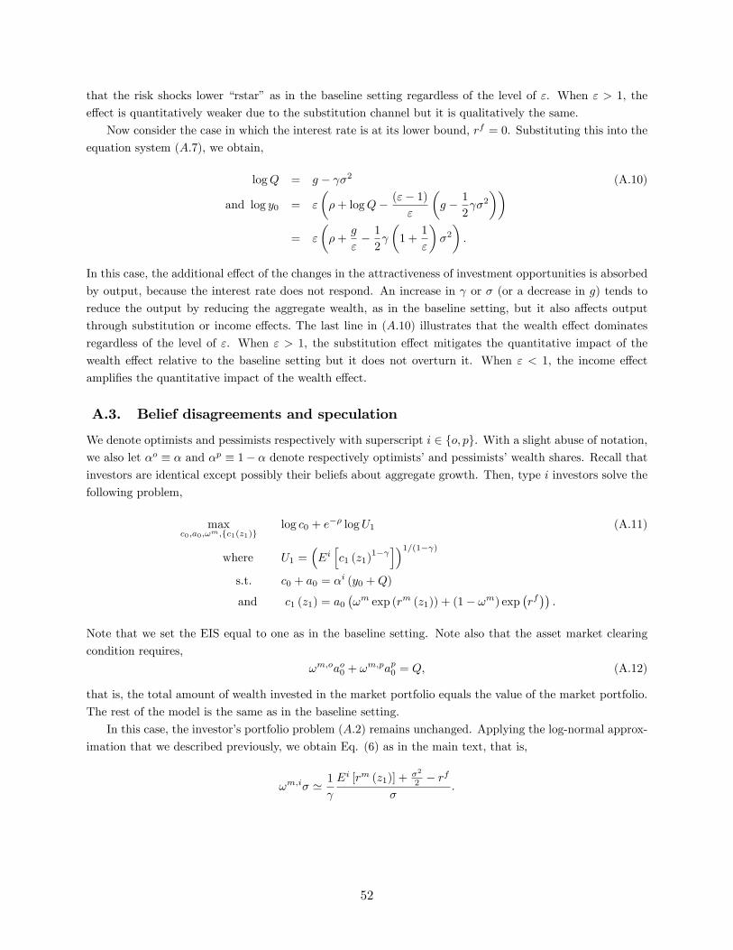
that the risk shocks lower “rstar” as in the baseline setting regardless of the level of ε. When ε > 1, the

effect is quantitatively weaker due to the substitution channel but it is qualitatively the same.

Now consider the case in which the interest rate is at its lower bound, rf = 0. Substituting this into the

equation system (A.7), we obtain,

logQ = g − γσ2 (A.10)

and log y0 = ε

(ρ+ logQ− (ε− 1)

ε

(g − 1

2γσ2

))= ε

(ρ+

g

ε− 1

2γ

(1 +

1

ε

)σ2).

In this case, the additional effect of the changes in the attractiveness of investment opportunities is absorbed

by output, because the interest rate does not respond. An increase in γ or σ (or a decrease in g) tends to

reduce the output by reducing the aggregate wealth, as in the baseline setting, but it also affects output

through substitution or income effects. The last line in (A.10) illustrates that the wealth effect dominates

regardless of the level of ε. When ε > 1, the substitution effect mitigates the quantitative impact of the

wealth effect relative to the baseline setting but it does not overturn it. When ε < 1, the income effect

amplifies the quantitative impact of the wealth effect.

A.3. Belief disagreements and speculation

We denote optimists and pessimists respectively with superscript i ∈ {o, p}. With a slight abuse of notation,we also let αo ≡ α and αp ≡ 1− α denote respectively optimists’and pessimists’wealth shares. Recall thatinvestors are identical except possibly their beliefs about aggregate growth. Then, type i investors solve the

following problem,

maxc0,a0,ωm,{c1(z1)}

log c0 + e−ρ logU1 (A.11)

where U1 =(Ei[c1 (z1)

1−γ])1/(1−γ)

s.t. c0 + a0 = αi (y0 +Q)

and c1 (z1) = a0(ωm exp (rm (z1)) + (1− ωm) exp

(rf)).

Note that we set the EIS equal to one as in the baseline setting. Note also that the asset market clearing

condition requires,

ωm,oao0 + ωm,pap0 = Q, (A.12)

that is, the total amount of wealth invested in the market portfolio equals the value of the market portfolio.

The rest of the model is the same as in the baseline setting.

In this case, the investor’s portfolio problem (A.2) remains unchanged. Applying the log-normal approx-

imation that we described previously, we obtain Eq. (6) as in the main text, that is,

ωm,iσ ' 1

γ

Ei [rm (z1)] + σ2

2 − rf

σ.

52

Substituting Ei [rm (z1)] = gi − logQ− σ2

2 [cf. Eq. (A.1)] into this expression, we further obtain,

ωm,iσ ' 1

γ

gi − logQ− rfσ

. (A.13)

As before, investors choose their share of the market portfolio so that their optimal portfolio risk is propor-

tional to the Sharpe ratio. The difference is that the Sharpe ratio is calculated according to investors’own

beliefs (and it is greater for optimists since go > gp).

The intertemporal problem (A.3) also remains unchanged. Taking the first order condition, we obtain,

ci0 =1

1 + e−ραi (y0 +Q) (A.14)

Aggregating this equation across investors, and using the aggregate resource constraint (3), shows that the

output-asset price relation (5) continues to apply in this setting. Belief heterogeneity does not affect this

equation since investors share the same discount rate, ρ.

Next note that combining (A.12) , (A.14) and (5), the asset market clearing condition can be rewritten

as,

αωm,o + (1− α)ωm,p = 1. (A.15)

Investors’wealth-weighted average portfolio weight on the market portfolio is equal to one. Combining this

with Eq. (A.13), we obtain the following analogue of Eq. (7),

σ ' 1

γ

αogo + αpgp − logQ− rfσ

. (A.16)

Hence, the risk balance condition continues to apply with the difference that the expected growth rate is

determined according to a weighted average belief. Another difference is that the condition is typically not

exact because investors’shares of the market portfolio typically deviate from one (and thus, their return is

typically not log-normal). Specifically, the equilibrium portfolio shares satisfy, ωo > 1 > ωp: optimists’make

a leveraged investment in the market portfolio by issuing some risk-free debt, whereas pessimists invest only

a fraction of their wealth in the market portfolio (and invest the rest of their wealth in the risk-free asset

issued by optimists).

Next consider the supply-determined equilibrium in which output is equal to its potential, y0 = z0 = 1.

By Eq. (5), this requires the asset price to be at a particular level, Q∗ = e−ρ. Combining this with Eq.

(A.16) we obtain Eq. (12) in the main text that characterizes “rstar.” The level of “rstar” is increasing

in optimists’wealth share, α. This is because increasing optimists’wealth share tends to increase asset

prices, aggregate demand, and output. In a supply-determined equilibrium, the monetary policy increases

the interest rate to neutralize the impact of optimists on aggregate demand and output.

Finally, consider the case in which the interest rate is at its lower bound, rf = 0. Substituting this into

the risk balance condition (A.16), and using the output-asset price relation (5), we obtain Eq. (9) in the

main text that characterizes the equilibrium level of output in a demand recession. In this case, increasing

optimists’wealth share translates into an actual increase in asset prices, aggregate demand, and output,

because the monetary policy cannot neutralize these effects due to the constraint on the interest rate.

53

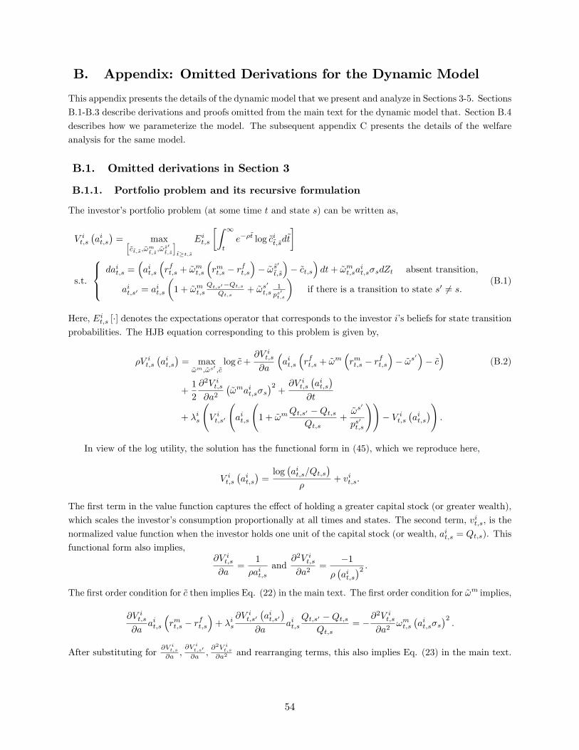
B. Appendix: Omitted Derivations for the Dynamic Model

This appendix presents the details of the dynamic model that we present and analyze in Sections 3-5. Sections

B.1-B.3 describe derivations and proofs omitted from the main text for the dynamic model that. Section B.4

describes how we parameterize the model. The subsequent appendix C presents the details of the welfare

analysis for the same model.

B.1. Omitted derivations in Section 3

B.1.1. Portfolio problem and its recursive formulation

The investor’s portfolio problem (at some time t and state s) can be written as,

V it,s(ait,s)

= max[ct,s,ω

mt,s,ωs′t,s

]t≥t,s

Eit,s

[∫ ∞t

e−ρt log cit,sdt

]

s.t.

dait,s =

(ait,s

(rft,s + ωmt,s

(rmt,s − r

ft,s

)− ωs

′

t,s

)− ct,s

)dt+ ωmt,sa

it,sσsdZt absent transition,

ait,s′ = ait,s

(1 + ωmt,s

Qt,s′−Qt,s

Qt,s+ ωs

′

t,s1ps′t,s

)if there is a transition to state s′ 6= s.

(B.1)

Here, Eit,s [·] denotes the expectations operator that corresponds to the investor i’s beliefs for state transitionprobabilities. The HJB equation corresponding to this problem is given by,

ρV it,s(ait,s)

= maxωm,ωs

′,c

log c+∂V it,s∂a

(ait,s

(rft,s + ωm

(rmt,s − r

ft,s

)− ωs

′)− c)

(B.2)

+1

2

∂2V it,s∂a2

(ωmait,sσs

)2+∂V it,s

(ait,s)

∂t

+ λis

(V it,s′

(ait,s

(1 + ωm

Qt,s′ −Qt,sQt,s

+ωs′

ps′t,s

))− V it,s

(ait,s)).

In view of the log utility, the solution has the functional form in (45), which we reproduce here,

V it,s(ait,s)

=log(ait,s/Qt,s

)ρ

+ vit,s.

The first term in the value function captures the effect of holding a greater capital stock (or greater wealth),

which scales the investor’s consumption proportionally at all times and states. The second term, vit,s, is the

normalized value function when the investor holds one unit of the capital stock (or wealth, ait,s = Qt,s). This

functional form also implies,∂V it,s∂a

=1

ρait,sand

∂2V it,s∂a2

=−1

ρ(ait,s)2 .

The first order condition for c then implies Eq. (22) in the main text. The first order condition for ωm implies,

∂V it,s∂a

ait,s

(rmt,s − r

ft,s

)+ λis

∂V it,s′(ait,s′

)∂a

ait,sQt,s′ −Qt,s

Qt,s= −

∂2V it,s∂a2

ωmt,s(ait,sσs

)2.

After substituting for∂V i

t,s

∂a ,∂V i

t,s′

∂a ,∂2V i

t,s

∂a2 and rearranging terms, this also implies Eq. (23) in the main text.

54

Finally, the first order condition for ωs′implies,

ps′

t,s

λis=

∂V it,s′(a

it,s′)

∂a

∂V it,s(ait,s)∂a

=1/ait,s′

1/ait,s,

which is Eq. (24) in the main text. This completes the characterization of the optimality conditions.

B.1.2. New Keynesian microfoundation for nominal rigidities

The supply side of our model features nominal rigidities similar to the standard New Keynesian setting.

There is a continuum of measure one of monopolistically competitive production firms denoted by ν. These

firms own the capital stock (in equal proportion) and produce differentiated goods, yt,s (ν), subject to the

technology,

yt,s (ν) = Aηt,s (ν) kt,s. (B.3)

Here, ηt,s (ν) ∈ [0, 1] denotes the firm’s choice of capital utilization. We assume utilization is free up to

ηt,s (ν) = 1 and infinitely costly afterwards. The production firms sell their output to a competitive sector

that produces the final output according to the CES technology,

yt,s =

(∫ 1

0

yt,s (ν)ε−1ε dν

)ε/(ε−1), (B.4)

for some ε > 1. Thus, the demand for the firms’goods implies,

yt,s (ν) ≤ pt,s (ν)−εyt,s, where pt,s (ν) = Pt,s (ν) /P . (B.5)

Here, pt,s (ν) denotes the firm’s relative price, which depends on its nominal price, Pt,s (ν), as well as the

ideal nominal price index, Pt,s =(∫

Pt,s (ν)1−ε

dν)1/(1−ε)

. We write the demand constraint as an inequality

because an individual firm can in principle refuse to meet the demand for its goods.

Without price rigidities, the firm chooses ηt,s (ν) ∈ [0, 1] , yt,s (ν) , pt,s (ν) to maximize its earnings,

pt,s (ν) yt,s (ν), subject to the supply constraint in (B.3) and the demand constraint, (B.5). In this case,

the demand constraint holds as equality (because otherwise the firm can always raise its price to keep its

production unchanged and raise its earnings). By combining the constraints, the firm’s problem can be

written as,

maxpt,s(ν),ηt,s(ν)

pt,s (ν)1−ε

yt,s s.t. 0 ≤ ηt,s (ν) =pt,s (ν)

−εyt,s

Akt,s≤ 1.

Inspecting this problem reveals that the solution features full factor utilization, ηt,s (ν) = 1. This is because,

when ηt,s (ν) < 1, the marginal cost of production is zero. Thus, the firm can always lower its price

and increase its demand and production, which in turn increases its earnings. Hence, at the optimum,

the firms set ηt,s (ν) = 1 and yt,s (ν) = Akt,s. To produce at this level, they set the relative price level,

pt,s (ν) =(yt,sAkt,s

)−1/ε. Since all firms are identical, we also have pt,s (ν) = 1 and yt,s = yt,s (ν) = Akt,s. In

particular, output is determined by aggregate supply at full factor utilization.

Now consider the alternative setting in which firms have a preset nominal price that is equal for all

firms, Pt,s (ν) = P . This also implies the relative price of a firm is fixed and equal to one, pt,s (ν) = 1.

The firm chooses the remaining variables, ηt,s (ν) ∈ [0, 1] , yt,s (ν), to maximize its earnings, yt,s (ν), subject

to the supply constraint in (B.3) and the demand constraint, (B.5). Combining the constraints and using

55

pt,s (ν) = 1, the firm’s problem can be written as,

maxηt,s(ν)

Aηt,s (ν) kt,s s.t. 0 ≤ ηt,s (ν) ≤ 1 and Aηt,s (ν) kt,s ≤ yt,s.

The solution is given by, ηt,s (ν) = min(

1,yt,sAkt,s

). Intuitively, when ηt,s (ν) < 1 and Aηt,s (ν) kt,s < yt,s, the

marginal cost of production is zero and there is some unmet demand for firms’goods. The firm optimally

increases its production until the supply or the demand constraints bind. Combining this observation with

the production technology for the final output, we also obtain, yt,s ≤ Akt,s. This implies that the demand

constraint holds as equality also in this case. In particular, we have ηt,s (ν) =yt,sAkt,s

≤ 1.

In sum, when the firms’nominal prices are fixed, aggregate output is determined by aggregate demand

subject to the capacity constraint, which verifies Eq. (19) in the dynamic model (and Eq. (3) in the two

period model).

Note also that, in equilibrium, firms’equilibrium earnings are equal to aggregate output, yt,s. Since firms

own the capital (and there is no rental market for capital), the division of these earnings between return to

capital and monopoly profits is indeterminate. This division does not play an important role in our baseline

model but it matters when we introduce investment. In Appendix D with endogenous investment (that we

present subsequently), we use slightly different microfoundations that ensure earnings accrue to firms in the

form of return to capital, i.e., there are no monopoly profits, which helps to simplify the exposition.

B.2. Omitted derivations in Section 4

Proof of Proposition 1. Provided in the main text.

B.3. Omitted derivations in Section 5

We derive the equilibrium conditions that we state and use in Section 5. First note that, using Eq. (24), the

optimality condition (23) can be written as,

ωm,it,s σs =1

σs

(rmt,s − r

ft,s + ps

′

t,s

Qt,s′ −Qt,sQt,s

). (B.6)

Note also that Eq. (25) implies,

ωm,ot,s = ωm,pt,s = 1. (B.7)

Next note that by definition, we have

aot,s = αt,sQt,skt,s and apt,s = (1− αt,s)Qt,skt,s for each s ∈ {1, 2} .

After plugging these into Eq. (24), using kt,s = kt,s′ (since capital does not jump), and aggregating over

optimists and pessimists, we obtain,

ps′

t,s = λt,sQt,sQt,s′

, (B.8)

where λt,s denotes the wealth-weighted average belief defined in (38).

Next, we combine Eqs. (B.6) , (B.7), and (B.8) to obtain

σs =1

σs

(rmt,s − r

ft,s + λt,s

(1− Qt,s

Qt,s′

))for each s ∈ {1, 2} . (B.9)

56

Substituting for rmt,s from Eq. (28), we obtain the risk balance condition (39) in the main text.

We next characterize investors’equilibrium positions. Combining Eq. (B.1) with Eqs. (B.7) and (B.8),

investors’wealth after transition satisfies,

ait,s′

ait,s=Qt,s′

Qt,s

(1 +

ωs′,it,s

λt,s

). (B.10)

From Eq. (24), we haveps′t,s

λis=

1/ait,s′

1/ait,s. Substituting this into the previous expression and using Eq. (B.8)

once more, we obtain,

ωs′,it,s = λis − λt,s for each i ∈ {o, p} . (B.11)

Combining this with Eq. (38) implies Eq. (40) in the main text.

Finally, we characterize the dynamics of optimists’wealth share. Combining Eqs. (B.10) and (B.11)

implies,

ait,s′

ait,s=

λisλt,s

Qt,s′

Qt,s. (B.12)

Combining this with the definition of wealth shares as well as kt,s = kt,s′ , we further obtain,

αt,s′

αt,s=

λosλt,s

. (B.13)

Thus, it remains to characterize the dynamics of wealth conditional on no transition. To this end, we combine

Eq. (B.1) with Eqs. (B.7) , (28) , (22) to obtain,

daot,saot,s

=(g + µQt,s − ω

s′,it,s

)dt+ σsdZt.

After substituting aot,s = αt,sQt,skt,s, and using the observation thatdQt,s

Qt,s= µQt,sdt and

dkt,skt,s

= gdt+ σsdZt,

we further obtain,dαt,sαt,s

= −ωs′,ot,s dt = −

(λos − λt,s

)dt. (B.14)

Combining Eqs. (B.13) and (B.14) implies Eq. (41) in the main text.

Proof of Proposition 2. First consider the high-risk-premium state, s = 2. Combining Eqs. (41) and

(42), we obtain the differential equation system,

qt,2 = −(ρ+ g + λ2 (αt,2)

(1− exp (q2)

Q∗

)− σ22

), (B.15)

αt,2 = − (λo2 − λp2)αt,2 (1− αt,2) .

This system describes the joint dynamics of the price and optimists’wealth share, (qt,2, αt,2), conditional on

there not being a transition. We next analyze the solution to this system using the phase diagram over the

range α ∈ [0, 1] and q2 ∈ [qp2 , qo2]. Here, recall that qi2 corresponds to the equilibrium log price with common

beliefs characterized in Section 4 corresponding to type i investors’belief.

First note that the system has two steady states given by, (αt,2 = 0, qt,2 = qp2), and (αt,2 = 1, qt,2 = qo2).

Next note that the system satisfies the Lipschitz condition over the relevant range. Thus, the vector flows

that describe the law of motion do not cross. Next consider the locus, q2 = 0. By comparing Eqs. (42)

57

Figure 8: The phase diagram that describes the equilibrium with heterogeneous beliefs.

and (33), this locus is exactly the same as the price that would obtain if investors shared the same wealth-

weighted average belief, denoted by q2 = qh2 (α). Using our analysis in Section 4, we also find that qh2 (α) is

strictly increasing in α. Moreover, q2 < qh2 (α) implies qt,2 < 0 whereas q2 > qh2 (α) implies qt,2 > 0. Finally,

note that αt,2 < 0 for each α ∈ (0, 1).

Combining these observations, the phase diagram has the shape in Figure 8. This in turn implies that

the system is saddle path stable. Given any αt,2 ∈ [0, 1), there exists a unique solution, qt,2, which ensures

that limt→∞ qt,2 = qp2 . We define the price function (the saddle path) as q2 (α). Note that the price function

satisfies q2 (α) < qh2 (α) for each α ∈ (0, 1), since the saddle path cannot cross the locus, qt,2 = 0. Note also

that q2 (1) = qo2, since the saddle path crosses the other steady-state, (αt,2 = 1, qt,2 = qo2). Finally, recall that

q2 < qh2 (α) implies qt,2 < 0. Combining this with αt,2 < 0, we further obtain dq2(α)dα > 0 for each α ∈ (0, 1).

Next note that, after substituting qt,2 = q′2 (α) αt,2, Eq. (B.15) implies the differential equation (43) in

α-domain. Thus, the above analysis shows there exists a solution to the differential equation with q2 (0) = qp2and q2 (1) = qo2. Moreover, the solution is strictly increasing in α, and it satisfies q2 (α) < qh2 (α) for each

α ∈ (0, 1). Note also that this solution is unique since the saddle path is unique. The last part of the

proposition follows from Eqs. (26) and (27).

Next consider the low-risk-premium state, s = 1. In the conjectured equilibrium, we have Qt,1 = Q∗,

which also implies µQt,1 = 0. Substituting these expressions into Eq. (39), we obtain the risk balance condition

in this state,

σ1 =1

σ1

(g + ρ− rft,1 + λt,1

(1− Q∗

Qt,2

)).

Writing the equilibrium variables as a function of optimists’ wealth share, we obtain rft,1 = rf1 (α) and

λt,1 = λ1 (α) and Qt,2 = exp (q2 (α′)), where α′ = αλo1/λ1 (α) denotes optimists’ wealth share after a

transition [cf. Eq. (41)]. Substituting these expressions into the risk balance condition and rearranging

terms, we obtain Eq. (44) in the main text that, which we replicate here,

rf1 (α) = ρ+ g − λ1 (α)

(Q∗

exp (q2 (α′))− 1

)− σ21.

58

Note also that drf1 (α)dα > 0 because λ1 (α) is decreasing in α (in view of Assumption 4), and q2 (α′) is

strictly increasing in α. The latter observation follows since α′ =αλo1

αλo1+(1−α)λp1is increasing in α (in view

of Assumption 4) and q2 (·) is a strictly increasing function. Note also that rf1 (α) > rf1 (0) > 0, where the

latter inequality follows since Assumptions 1-3 holds for the pessimistic belief. Thus, the interest rate in

state 1 is always positive, which verifies our conjecture and completes the proof.

B.4. Details of the parameterization

This section describes the details of the parameterization of the dynamic model that we use to numerically

illustrate our findings. This parameterization is only meant to be reasonable, as its purpose is to give a sense

of potential magnitudes. Throughout, we measure time in years so that the continuous-time rates we choose

correspond to (approximate) yearly rates.

Since we do not explicitly model steady-state inflation (for simplicity), we interpret the growth rate in

our model as g = g + π where g can be thought of as the real growth rate and π ≥ 0 can be thought of

as the steady-state inflation. With this adjustment, we can interpret the returns in our model as capturing

the corresponding nominal returns in the data. In particular, the zero lower bound constraint in the model

(20) becomes a restriction on the nominal risk-free rate (as in the data). We set π = 2% based on the Fed’s

inflation target in recent decades; and g = 3% based on pre-recession estimates for the U.S. trend output

growth, which leads to:

g = 5%.

For the discount rate, we set,

ρ = 4%,

based on the yearly discount rates typically assumed in the literature. This implies a first-best (nominal)

return to capital given by rm,∗ = ρ+ r = 9% [cf. (30)], which is consistent with the historical estimates for

the weighted-average return on stocks and housing in Jordà et al. (2019).

We set the variance in the low-risk-premium state to target the first-best nominal risk-free interest rate

in the boom given by, rf,∗1 = 4% (equivalently, a real risk-free rate given by 2%), which is consistent with

the low interest rates in recent years. Using (31), this leads to:

σ21 = 5%.

We set the variance in the high-risk-premium state to target a first-best interest rate rf,∗2 = −1%, which

leads to:

σ22 = 10%.

These choices (together with the choices of ρ and g) ensure that Assumption 1 holds. For the productivity

level, we set A = 1. This does not play a role as it scales all variables.

It remains to set investors’beliefs for transition probabilities,(λis)s∈{1,2},i∈{o,p}. We set:

λo1 = 1/10 and λo2 = 1/3,

λp1 = 1/3 and λp2 = 1/10.

Hence, optimists think a boom lasts on average 10 years whereas pessimists think it lasts for only three years

(and vice versa for the recession).

59

C. Appendix: Omitted Derivations for the Welfare Analysis

This appendix presents the omitted derivations and proofs for the welfare analysis of the dynamic model

that we present in Section 6. Section C.1 establishes the properties of the equilibrium value functions that

are used in the main text. Section C.2 describes the details of the equilibrium with macroprudential policy,

presents the analyses omitted from the main text (e.g., macroprudential policy in the high-risk-premium

state), and presents omitted proofs.

C.1. Value functions in equilibrium

We first derive the HJB equation that describes the normalized value function in equilibrium and derive

Eqs. (46). We then derive the differential equations in α-domain that characterize the value function and

its components, and derive Eq. (49). We then prove Lemmas 1 and 2 that are used in the analysis.

Characterizing the normalized value function in equilibrium. Consider the recursive version

of the portfolio problem in (B.2). Recall that the value function has the functional form in Eq. (45). Our

goal is to characterize the value function per unit of capital, vit,s (corresponding to ait,s = Qt,s). To facilitate

the analysis, we define,

ξit,s = vit,s −logQt,s

ρ. (C.1)

Note that ξit,s is the value function per unit wealth (corresponding to ait,s = 1), and that the value function

also satisfies V it,s(ait,s)

=log(ait,s)

ρ + ξit,s. We first characterize ξit,s. We then combine this with Eq. (C.1) to

characterize our main object of interest, vit,s.

Consider the HJB equation (B.2). We substitute the optimal consumption rule from Eq. (22), the

contingent allocation rule from Eq. (24), and ait,s = 1 (to characterize the value per unit wealth) to obtain,

ρξit,s = log ρ+1

ρ

(rft,s + ωm,it,s

(rmt,s − r

ft,s

)− 1

2

(ωm,it,s

)2σ2s − ρ− ω

s′,it,s

)(C.2)

+∂ξit,s∂t

+ λis

(1

ρlog

(λisps′t,s

)+ ξit,s′ − ξit,s

).

As we describe in Section 5, the market clearing conditions imply the optimal investment in the market

portfolio and contingent securities satisfies, ωm = 1 and ωs′,it,s = λis − λt,s, and the price of the contingent

security is given by, ps′

t,s = λt,s1/Qt,s′

1/Qt,s. Here, λt,s denotes the weighted average belief defined in (38). Using

these conditions, the HJB equation becomes,

ρξit,s = log ρ+1

ρ

(rmt,s − ρ− 1

2σ2s

−(λis − λt,s

)+ λis log

(λisλt,s

) ) (C.3)

+∂ξit,s∂t

+ λis

(1

ρlog

(Qt,s′

Qt,s

)+ ξit,s′ − ξit,s

).

After substituting the return to the market portfolio from (28), the HJB equation can be further simplified

60

as,

ρξit,s =log ρ+ 1

ρ

(g + µQt,s − 1

2σ2s

−(λis − λt,s

)+ λis log

(λisλt,s

) )+∂ξit,s∂t + λis

(1ρ log

(Qt,s′

Qt,s

)+ ξit,s′ − ξit,s

) .

Here, the term inside the summation on the second line, −(λis − λt,s

)+λis log

(λisλt,s

), is zero when there are

no disagreements, and it is strictly positive when there are disagreements. This illustrates that speculation

increases the expected value for optimists as well as pessimists.

We finally substitute vit,s = ξit,s +logQt,s

ρ (cf. (C.1)) into the HJB equation to obtain the differential

equation,

ρvit,s =log ρ+ log (Qt,s) + 1

ρ

(g − 1

2σ2s

−(λis − λt,s

)+ λis log

(λisλt,s

) )+∂vit,s∂t + λis (vt,s′ − vt,s)

.

Here, we have canceled terms by using the observation that∂ξit,s∂t =

∂vit,s∂t −

1ρ∂ logQt,s

∂t =∂vit,s∂t −

1ρµ

Qt,s. We

have thus obtained Eq. (46) in the main text.

Differential equations for the value functions in α-domain. The value function and its compo-

nents,{vit,s, v

i,∗t,s , wt,s

}s,i, can be written as functions of optimists’wealth share,

{vis (α) , vi,∗s (α) , ws (α)

}s,i,

that solve appropriate ordinary differential equations. We next represent the value functions as solutions to

the differential equations in α-domain. Recall that the price level in each state can be written as a function

of optimists’wealth shares, qt,s = qs (α) (where we also have, q1 (α) = q∗). Plugging in these price functions,

and using the dynamics of αt,s from Eq. (41), the HJB equation (46) can be written as,

ρvis (α) =log ρ+ qs (α) + 1

ρ

(g − 1

2σ2s

−(λis − λs (α)

)+ λis log

(λis

λs(α)

) )−∂v

is

∂α (λos − λps)α (1− α) + λis

(vis′(α

λosλs(α)

)− vis (α)

) .

For each i ∈ {o, p}, the value functions,(vis (α)

)s∈{1,2}, are found by solving this system of ODEs. For i = o,

the boundary conditions are that the values, {vos (1)}s, are the same as the values in the common beliefbenchmark characterized in Section 4 when all investors have the optimistic beliefs. For i = p, the boundary

conditions are that the values, {vps (0)}s, are the same as the values in the common belief benchmark whenall investors have the pessimistic beliefs.

Likewise, the first-best value functions,(vi,∗s (α)

)s∈{1,2}, are found by solving the analogous system after

replacing qs (α) with q∗ (and changing the boundary conditions appropriately). Finally, substituting the

price functions into Eq. (48), the gap-value functions,(wis (α)

)s,i, are found by solving the system in (49).

For the proofs in this section (as well as in some subsequent sections), we find it useful to work with the

transformed state variable,

bt,s ≡ log

(αt,s

1− αt,s

), which implies αt,s =

1

1 + exp (−bt,s). (C.4)

The variable, bt,s, varies between (−∞,∞) and provides a different measure of optimism, which we refer to

as “bullishness.”Note that there is a one-to-one relation between optimists’wealth share, αt,s ∈ (0, 1), and

61

the bullishness, bt,s ∈ R = (−∞,+∞). Optimists’wealth dynamics in (41) become particularly simple when

expressed in terms of bullishness,{bt,s = − (λos − λps) , if there is no state change,

bt,s′ = bt,s + log λos − log λps , if there is a state change.(C.5)

With a slight abuse of notation, we also let q2 (b) , wis (b), and so on, denote the equilibrium functions in

terms of bullishness. Note also that, since dbdα = 1

α(1−α) , we have the identities,

∂q2 (b)

∂b= α (1− α)

∂q2 (α)

∂band

∂wis (b)

∂b= α (1− α)

∂wis (α)

∂α. (C.6)

Using this observation, the differential equation for the price function, Eq. (43), can be written in terms of

bullishness as,

∂q2 (b)

∂b(λo2 − λ

p2) = ρ+ g + λ2 (α)

(1− Q2

Q∗

)− σ22. (C.7)

Likewise, the differential equation for the gap value function, Eq. (49), can be written in terms of bullishness

as,

ρwis (b) = qs (b)− q∗ − (λos − λps)∂wis (b)

∂b+ λis

(wis′ (b

′)− wis (b)). (C.8)

Proof of Lemma 1. To show that the gap value function is increasing, consider its representation in termsof bullishness, wis (b) [cf. (C.4)], which solves the system in (C.8). We will first describe this function as a

fixed point of a contraction mapping. We will then use this contraction mapping to establish the properties

of the function.

Recall that, in the time domain, the gap value function solves the HJB equation (48). Integrating this

equation forward, we obtain,

wis (b0,s) =

∫ ∞0

e−(ρ+λis)t(qs (bt,s)− q∗ + λisw

is′ (bt,s′)

)dt, (C.9)

for each s ∈ {1, 2} and b0,s ∈ R. Here, bt,s denotes bullishness conditional on there not being a transitionbefore time t, whereas bt,s′ denotes the bullishness if there is a transition at time t. Solving Eq. (C.5) (given

beliefs, λi) we further obtain,

bt,s = b0,s − t (λos − λps) , (C.10)

bt,s′ = b0,s − t (λos − λps) + log λos − log λps .

Hence, Eq. (C.9) describes the value function as a solution to an integral equation given the closed form

solution for bullishness in (C.10).

Implicitly differentiating the integral equation (C.9) with respect to b0,s, and using Eq. (C.10), we also

obtain,∂wis (b0,s)

∂b=

∫ ∞0

e−(ρ+λis)t(∂qs (bt,s)

∂b+ λis

∂wis′ (bt,s′)

∂b

)dt. (C.11)

We next let B(R2)denote the set of bounded value functions over R2. Given some continuation value

62

function,(∂wis(b)∂b

)s∈ B

(R2), we define the function,

(T∂wis(b)∂b

)s∈ B

(R2), so that

T∂wis (b0,s)

∂b=

∫ ∞0

e−(ρ+λis)t(∂qs (bt,s)

∂b+ λis

∂wis′ (bt,s′)

∂b

)dt,

for each s and b0,s ∈ R. Note also that the resulting value functions are bounded since the derivative ofthe price functions,

(∂qs(bt,s)

∂b

)s, are bounded (see Eq. (C.7)). Thus, Eq. (C.11) describes the derivative

functions,(∂wis(b0,s)

∂b

)s, as a fixed point of a corresponding operator T over bounded functions. It can be

checked that this operator is a contraction mapping with respect to the sup norm. Thus, it has a unique

fixed point that corresponds to the derivative functions. Moreover, since ∂qs(bt,s)∂b > 0 for each b, and λis > 0

for each s, it can further be seen that the fixed point satisfies, ∂wis(b0,s)∂b > 0 for each b and s ∈ {1, 2}. Using

Eq. (C.6), we also obtain ∂wis(α)∂α > 0 for each α ∈ (0, 1) and s ∈ {1, 2}, completing the proof.

Proof of Lemma 2. Consider the analysis in Lemma 1 for the special case, λo1 = λp1. Applying Eq. (C.11)

for s = 1, we obtain [since q1 (bt,s) = q∗ is constant],

∂wi1 (b0,1)

∂b=

∫ ∞0

e−(ρ+λi1)tλi1∂wi2 (bt,2)

∂bdt.

Note also that λo1 = λp1 and Eq. (C.10) imply bt,2 = b0,1 (since there is no speculation). Substituting this

into the displayed equation, we obtain ∂wi1(b0,1)∂b =

λi1ρ+λi1

∂wi2(b0,1)∂b <

∂wi2(b0,1)∂b . Combining this with Eq. (C.6)

completes the proof.

C.2. Equilibrium with macroprudential policy

Recall that macroprudential policy induces optimists to choose allocations as if they have more pessimistic

beliefs, λo,pl ≡(λo,pl1 , λo,pl2

), that satisfy, λo,pl1 ≥ λo1 and λ

o,pl2 ≤ λo2. We next show that this allocation can

be implemented with portfolio restrictions on optimists. We then show that the planner’s Pareto problem

reduces to solving problem (51) in the main text. We also derive the equilibrium value functions that

result from macroprudential policy. We then analyze macroprudential policy in the recession state, which

complements the analysis in the main text (that focuses on the boom state), and present Proposition 4.

Finally, we present the proofs of Propositions 3 and 4.

Implementing the policy with risk limits. Consider the equilibrium that would obtain if optimists

had the planner-induced beliefs, λo,pls . Using our analysis in Section 5, optimists’equilibrium portfolios are

given by,

ωm,o,plt,s = 1 and ωs′,o,plt,s = λo,pls − λplt,s for each t, s. (C.12)

We first show that the planner can implement the policy by requiring optimists to hold exactly these portfolio

weights. We will then relax these portfolio constraints into inequality restrictions (see Eq. (C.14)).

Formally, an optimist solves the HJB problem (B.2) with the additional constraint (C.12). In view of

log utility, we conjecture that the value function has the same functional form (45) with potentially different

normalized values, ξot,s, vot,s, that reflect the constraints. Using this functional form, the optimality condition

for consumption remains unchanged, ct,s = ρaot,s [cf. Eq. (22)]. Plugging this equation and the portfolio

holdings in (C.12) into the objective function in (B.2) verifies that the value function has the conjectured

functional form. For later reference, we also obtain that the optimists’unit-wealth value function satisfies

63

[cf. Eq. (C.1)],

ξot,s = log ρ+1

ρ

(rft,s + ωm,o,plt,s

(rmt,s − r

ft,s

)− ρ− ωs

′,o,plt,s

)(C.13)

− 1

2ρ

(ωm,o,plt,s σs

)2+∂ξot,s∂t

+ λos

(1

ρlog

(aot,s′

aot,s

)+ ξot,s′ − ξot,s

).

Here,aot,s′

aot,s= 1+ωm,o,plt,s

Qt,s′−Qt,s

Qt,s+ωs′,o,plt,s

ps′t,s

in view of the budget constraints (B.1). Hence, the value function

has a similar characterization as before [cf. Eq. (C.2)] with the difference that optimists’portfolio holdings

reflect the portfolio constraints.

Since pessimists are unconstrained, their optimality conditions are unchanged. It follows that the equi-

librium takes the form in Section 5 with the difference that investors’beliefs are replaced by their as-if beliefs,

λi,pls . This verifies that the planner can implement the policy using the portfolio restrictions in (C.12). We

next show that these restrictions can be relaxed to the following inequality constraints,

ωm,o,plt,s ≤ 1 for each s, (C.14)

ω2,o,plt,1 ≥ ω2,ot,1 ≡ λo,pl1 − λplt,1 and ω

1,o,plt,2 ≤ ω1,ot,2 ≡ λ

o,pl2 − λplt,2.

In particular, we will establish that all inequality constraints bind, which implies that optimists optimally

choose the portfolio weights in Eq. (C.12). Thus, our earlier analysis continues to apply when optimists are

subject to the more relaxed restrictions in (C.14).

The result follows from the assumption that the planner-induced beliefs are more pessimistic than opti-

mists’actual beliefs, λo,pl1 ≥ λo1 and λo,pl2 ≤ λo2. To see this formally, note that the optimality condition for

the market portfolio is given by the following generalization of Eq. (23),

ωm,o,plt,s σs ≤1

σs

(rmt,s − r

ft,s + λos

aot,saot,s′

Qt,s′ −Qt,sQt,s

)and ωm,o,plt,s ≤ 1, (C.15)

with complementary slackness. Note also that,

λosaot,saot,s′

Qt,s′ −Qt,sQt,s

= λosλpl

t,s

λo,pls

Qt,s′ −Qt,sQt,s′

≥ λplt,sQt,s′ −Qt,s

Qt,s′for each s.

Here, the equality follows because Eq. (B.12) in Appendix B.3 applies with as-if beliefs. The inequality

follows by considering separately the two cases, s ∈ {1, 2}. For s = 2, the inequality holds since Qt,s′−Qt,s >0 and the beliefs satisfy, λos ≥ λo,pls . For s = 1, the inequality holds since Qt,s′ − Qt,s < 0 and the beliefs

satisfy, λo,pls ≥ λos. Note also that in equilibrium the return to the market portfolio satisfies Eq. (B.9), which

we replicate here,

σs =1

σs

(rmt,s − r

ft,s + λ

pl

t,s

(1− Qt,s

Qt,s′

)).

Combining these expressions implies, σs ≤ 1σs

(rmt,s − r

ft,s + λos

aot,saot,s′

Qt,s′−Qt,s

Qt,s

), which in turn implies the

optimality condition (C.15) is satisfied with ωm,o,plt,s = 1. A similar analysis shows that optimists also choose

the corner allocations in contingent securities, ω2,o,plt,1 = ω2,ot,1 and ω1,o,plt,2 = ω1,ot,2 , verifying that the portfolio

constraints (C.12) can be relaxed to the inequality constraints in (C.14).

64

Simplifying the planner’s problem. Recall that, to trace the Pareto frontier, we allow the planner to

do a one-time wealth transfer among the investors at time 0. Let V it,s(ait,s|

{λo,plt

})denote type i investors’

expected value in equilibrium when she starts with wealth ait,s and the planner commits to implement the

policy,{λo,plt

}. Then, the planner’s Pareto problem can be written as,

maxλo,pl

,α0,s

γoV o0,s

(α0,sQ0,sk0,s|λ

o,pl)

+ γpV p0,s

((1− α0,s)Q0,sk0,s|λ

o,pl). (C.16)

Here, γo, γp ≥ 0 (with at least one strict inequality) denote the Pareto weights, and Q0,s denotes the

endogenous equilibrium price that obtains under the planner’s policy.

Next recall that the investors’value function with macroprudential policy has the same functional form

in (45) (with potentially different ξot,s, vot,s for optimists that reflect the constraints). After substituting

ait,s = αit,skt,sQt,s, the functional form implies,

V it,s = vit,s +log(αit,s

)+ log (kt,s)

ρ.

Using this expression, the planner’s problem (C.16) can be rewritten as,

maxλo,pl

,α0,s

(γovo0,s + γpvp0,s

)+γo log

(αo0,s

)+ γp log

(1− αo0,s

)ρ

+(γo + γp) log (k0,s)

ρ.

Here, the last term (that features capital) is a constant that doesn’t affect optimization. The second term

links the planner’s choice of wealth redistribution, αo0,s, αp0,s, to her Pareto weights, γ

o, γp. Specifically, the

first order condition with respect to optimists’wealth share implies γo

γp =α0,s1−α0,s . Thus, the planner effectively

maximizes the first term after substituting γo and γp respectively with the optimal choice of α0,s and 1−α0,s.This leads to the simplified problem (51) in the main text.

Characterizing the value functions with macroprudential policy. We first show that the

normalized value functions, vit,s, are characterized as the solution to the following differential equation system,

ρvit,s −∂vit,s∂t

= log ρ+ qt,s +1

ρ

g − 12σ

2s

−(λi,pls − λplt,s

)+ λis log

(λi,pls

λplt,s

) + λis(vit,s′ − vit,s

). (C.17)

This is a generalization of Eq. (46) in which investors’positions are calculated according to their as-if beliefs,

λi,pls , but the transition probabilities are calculated according to their actual beliefs, λis.

First consider the pessimists. Since they are unconstrained, their value function is characterized by

solving the earlier equation system (C.13). In this case, equation (C.17) also holds since it is the same as

the earlier equation.

Next consider the optimists. In this case, the analysis in Appendix B.3 applies with as-if beliefs. In

particular, we have [cf. Eqs. (B.12) and (B.13)],

aot,s′

aot,s=λo,pls

λpl

t,s

Qt,s′

Qt,s.

65

Plugging this expression as well as Eq. (C.12) into Eq. (C.13), optimists’unit-wealth value function satisfies,

ξot,s = log ρ+1

ρ

rmt,s − ρ− 12σ

2s

−(λo,pls − λplt,s

)+ λos log

(λo,plt,s

λplt,s

) +∂ξot,s∂t

+ λos

(1

ρlog

(Qt,s′

Qt,s

)+ ξot,s′ − ξot,s

),

This is the same as Eq. (C.13) with the difference that the as-if beliefs, λo,pls , are used to calculate their

positions on (and the payoffs from) the contingent securities, whereas the actual beliefs, λos, are used to

calculate the transition probabilities. Using the same steps after Eq. (C.13), we also obtain (C.17) with

i = o.

We next characterize the first-best and the gap value functions, vi,∗t,s and wit,s, that we use in the main

text. By definition, the first-best value function solves the same differential equation (C.17) after substituting

qt,s = q∗. It follows that the gap value function wit,s = vit,s − vi,∗t,s , solves,

ρwit,s −∂wit,s∂t

= qt,s − q∗ + λis(wit,s′ − wit,s

),

which is the same as the differential equation (48) without macroprudential policy. The latter affects the

path of prices, qt,s, but it does not affect how these prices translate into gap values.

Note also that, as before, the value functions can be written as functions of optimists’wealth share,{vis (α) , vi,∗s (α) , ws (α)

}s,i. For completeness, we also characterize the differential equations that these

functions satisfy in equilibrium with macroprudential policy. Combining Eq. (C.17) with the dynamics of

optimists’wealth share conditional on no transition, αt,s = −(λo,pls − λps

)αt,s (1− αt,s), the value functions,(

vis (α))s,i, are found by solving,

ρvis (α) =

log ρ+ qpls (α) + 1

ρ

g − 12σ

2s

−(λi,pls − λplt,s

)+ λis log

(λi,pls

λplt,s

) −∂v

is

∂α

(λo,pls − λps

)α (1− α) + λis

(vis′

(αλo,pls

λplt,s

)− vis (α)

) ,

with appropriate boundary conditions. As in the main text, we denote the price functions with qpls (α) to

emphasize that they are determined by as-if beliefs. Likewise, the first-best value functions,(vi,∗s (α)

)s∈{1,2},

are found by solving the analogous system after replacing qs (α) with q∗. Finally, combining Eq. (48) with

the dynamics of optimists’wealth share, the gap-value functions,(wis (α)

)s,i, are found by solving Eq. (50)

in the main text

Macroprudential policy in the recession state. The analysis in the main text concerns macro-

prudential policy in the boom state and maintains the assumption that λo,pl2 = λo2. We next consider the

polar opposite case in which the economy is currently in the recession state s = 2, and the planner can

apply macroprudential policy in this state, λo,pl2 ≤ λo2 (she can induce optimists to act as if the recovery is

less likely), but not in the other state, λo,pl1 = λo1. We obtain a sharp result for the special case in which

optimists’wealth share is suffi ciently large.

66

Proposition 4. Consider the model with two belief types. Consider the macroprudential policy in the

recession state, λo,pl2 ≤ λo2 (and suppose λo,pl1 = λo1). There exists a threshold, α < 1, such that if α ∈ (α, 1],

then the policy reduces the gap value according to each belief, that is,

∂wi2 (α)

∂(−λo,pl2

)∣∣∣∣∣∣λo,pl2 =λo2

< 0 for each i ∈ {o, p} .

Thus, for α ∈ (α, 1], the policy also reduces the planner’s value, ∂vpls (α)

∂(−λo,pl2 )

∣∣∣∣λo2

=∂wpls (α)

∂(−λo,pl2 )

∣∣∣∣λo2

< 0.

Thus, in contrast to Proposition 3, macroprudential policy in the recession state can actually reduce

the gap value (and therefore also the social welfare). The intuition can be understood by considering two

counteracting forces. First, as before, macroprudential policy in the recession state is potentially valuable by

reallocating optimists’wealth from the boom state s = 1 to the recession state s = 2. Intuitively, optimists

purchase too many call options that pay if there is a transition to the boom state but that impoverish them

in case the recession persists. They do not internalize that, if they keep their wealth, they will improve asset

prices if the recession lasts longer.

However, there is a second force that does not have a counterpart in the boom state: Macroprudential

policy in the recession state also affects the current asset price level, with potential implications for gap value.

It can be seen that making optimists less optimistic in the recession state shifts the price function downward,∂qpl2 (α)

∂(−λo,pl2 )< 0 (as in the common-belief benchmark we analyzed in Section 4). Hence, the price impact of

macroprudential policy reduces the gap value. Moreover, as optimists dominate the economy, α → 1, the

price impact of the policy is still first order, whereas the beneficial effect from reshuffl ing optimists’wealth

is second order. Thus, when optimists’wealth share is suffi ciently large, the net effect of macroprudential

policy on the gap value is negative.

This analysis also suggests that, even when the policy in the recession state exerts a net positive effect,

it would typically increase the gap value by a smaller amount than a comparable policy in the boom state.

Figure 9 confirms this intuition. The left panel plots the change in the planner’s gap value function in the

boom state resulting from a small macroprudential policy change. Note that the policy slightly reduces the

planner’s first-best value function but increases the gap value function. The right panel illustrates the effect

of the macroprudential policy in the recession state that would generate a similar distortion in the first-best

equilibrium as the policy in the boom state.30 Note that a small macroprudential policy in the recession

state has a smaller positive impact on the gap value when optimists’wealth share is small, and it has a

negative impact when optimists’wealth share is suffi ciently large, illustrating Proposition 4.

Proof of Proposition 3. We will prove the stronger result that

∂wis (α)

∂λo,pl1

∣∣∣∣∣λo,pl=λo

> 0 for each i, s and α ∈ (0, 1) . (C.18)

That is, a marginal amount of macroprudential policy in the low-risk-premium state increases the gap value

according to each investor (and in either state). Combining this with the definition of the planner’s gap

value function in (52) implies ∂wpls (α)

∂λo,pl1

∣∣∣λo,pl=λo

> 0. Combining this with∂vpl,∗0,s

∂λo,pl

∣∣∣∣λo,pl=λo

= 0 (which follows

30Specifically, we calibrate the policy-induced belief change in the recession state so that the maximum decline in the

planner’s first-best value function is the same in both cases plotted in Figure 9, maxα

∣∣∣∆vpl,∗2 (α)∣∣∣ = maxα

∣∣∣∆vpl,∗1 (α)∣∣∣.

67

0 0.2 0.4 0.6 0.8 1

­0.0006

­0.0005

­0.0004

­0.0003

­0.0002

­0.0001

      0

 0.0001

 0.0002

 0.0003

 0.0004

0 0.2 0.4 0.6 0.8 1

­0.0006

­0.0005

­0.0004

­0.0003

­0.0002

­0.0001

      0

 0.0001

 0.0002

 0.0003

 0.0004

Figure 9: The left (resp. the right) panel illustrates the effect of a small change in macroprudentialpolicy in the boom (resp. the recession) state.

from the First Welfare Theorem) and vpl0,s = vpl,∗0,s + wpl0,s implies∂wpls (α)

∂λo,pl1

∣∣∣λo,pl=λo

=∂vpls (α)

∂λo,pl1

∣∣∣λo,pl=λo

for each

s and α ∈ (0, 1). Applying this result for state s = 1 proves the proposition.

It remains to prove the claim in (C.18). To this end, fix a belief type i and consider the representation

of the gap value function in terms of bullishness, wis (b) [cf. (C.4)]. Following similar steps as in Lemma 1,

we describe this as solution to the integral function,

wis (b0,s) =

∫ ∞0

e−(ρ+λis)t(qpls (bt,s)− q∗ + λisw

is′ (bt,s′)

)dt, (C.19)

for each s ∈ {1, 2} and b0,s ∈ R, where the bullishness has the closed form solution,

bt,s = b0,s − t(λo,pls − λps

), (C.20)

bt,s′ = b0,s − t(λo,pls − λps

)+ log λo,pls − log λps .

The main difference from the analysis in Lemma 1 is that the dynamics of bullishness is influenced by

policy, as illustrated by the as-if beliefs in (C.10). In addition, we denote the price functions with qpls (b) to

emphasize they are in principle determined by as-if beliefs.

Next note that in this case the price functions qpls (b) are actually not affected by the as-if belief, λo,pl1 .

The price function in the low-risk-premium state is not affected because qpl1 (b) = q∗ (because the beliefs

continue to satisfy Assumption 3 for small changes). The price function in the high-risk-premium state is

also not affected because λo,pl1 does not enter the differential equation that characterizes qpl2 (b) [see. Eq.

(43) or Eq. (C.7)].

Using this observation, we implicitly differentiate the integral equation (C.19) with respect to λo,pl1 , and

68

use Eq. (C.20), to obtain,

∂wi1 (b0,1)

∂λo,pl1

=

∫ ∞0

e−(ρ+λi1)tλi1

(∂wi2 (bt,2)

∂λo,pl1

+∂wi2 (bt,2)

∂b

dbt,2

dλo,pl1

)dt,

∂wi2 (b0,2)

∂λo,pl1

=

∫ ∞0

e−(ρ+λi1)tλi2∂wi1 (bt,1)

∂λo,pl1

dt.

Note also that, using Eq. (C.20) implies, dbt,2

dλo,pl1

= −t + 1

λo,pl1

. Plugging this into the previous system, and

evaluating the partial derivatives at λo,pl1 = λo1, we obtain,

∂wi1 (b0,1)

∂λo,pl1

= h (b0,1) +

∫ ∞0

e−(ρ+λi1)tλi1∂wi2 (bt,2)

∂λo,pl1

dt, (C.21)

∂wi2 (b0,2)

∂λo,pl1

=

∫ ∞0

e−(ρ+λi1)tλi2∂wi1 (bt,1)

∂λo,pl1

dt,

where h (b0,1) =

∫ ∞0

e−(ρ+λi1)tλi1∂wi2 (bt,2)

∂b

(−t+

1

λo1

)dt.

Note that the function, h (b), is bounded since the derivative function, ∂wi2(b)∂b , is bounded (see (C.11)). Hence,

Eq. (C.21) describes the partial derivative functions,(∂wis(b)

∂λo,pl1

|λo,pl1 =λo1

)s, as a fixed point of a corresponding

operator T over bounded functions. Since h (b) is bounded, it can be checked that the operator T is also a

contraction mapping with respect to the sup norm. In particular, it has a fixed point, which corresponds to

the partial derivative functions.

The analysis so far applies generally. We next consider the special case, λo1 = λp1, and show that it implies

the partial derivatives are strictly positive. In this case, λi1 ≡ λ1 for each i ∈ {o, p}. In addition, Eq. (C.10)

implies bt,2 = b0,2. Using these observations, for each b0,1, we have,

h (b0,1) =∂wi2 (b0,2)

∂b

∫ ∞0

e−(ρ+λ1)tλ1

(−t+

1

λ1

)dt

=∂wi2 (b0,2)

∂b

(− λ1ρ+ λ1

1

ρ+ λ1+

1

ρ+ λ1

)> 0.

Here, the inequality follows since ∂wi2(b0,2)∂b > 0 [cf. Lemma 1]. Since h (b) > 0 for each b, and λis > 0, it can

further be seen that the fixed point that solves (C.21) satisfies ∂wis(b)

∂λo,pls> 0 for each b and s ∈ {1, 2}. Using

Eq. (C.6), we also obtain∂wis(α)

∂λo,pl1

> 0 for each s ∈ {1, 2} and α ∈ (0, 1). Since the analysis applies for any

fixed belief type i, this establishes the claim in (C.18) and completes the proof.

Proof of Proposition 4. A similar analysis as in the proof of Proposition 3 implies that the partial

derivative function, ∂wis(b)

∂(−λo,pl2 ), is characterized as the fixed point of a contraction mapping over bounded

functions (the analogue of Eq. (C.21) for state 2). In particular, the partial derivative exists and it is

bounded. Moreover, since the corresponding contraction mapping takes continuous functions into continuous

functions, the partial derivative is also continuous over b ∈ R. Using Eq. (C.6), we further obtain that the

partial derivative, ∂wis(α)

∂(−λo,pl2 ), is continuous over α ∈ (0, 1).

Next note that wis (1) ≡ limα→1 wis (α) exists and is equal to the value function according to type i beliefs

when all investors are optimistic. In particular, the asset prices are given by qpl1 = q∗ and qpl2 = qo, and the

69

transition probabilities are evaluated according to type i beliefs. Then, following the same steps as in our

analysis of value functions in Appendix C.1, we obtain,

ρwis (1) = βisqos +

(1− βis

)qos′ − q∗,

where βis =ρ+ λis′

ρ+ λis′ + λis.

Here, βis can be thought of as the expected discount time the investor spends in state s according to type i

beliefs. We consider this equation for s = 2 and take the derivative with respect to(−λo,pl2

)to obtain,

∂wi2 (1)

∂(−λo,pl2

) = βi2dqo2

d(−λo,pl2

) < 0.

Here, the inequality follows since reducing optimists’optimism reduces the price level in the common belief

benchmark (see Section 4).

Note that the inequality, ∂wi2(1)

∂(−λo,pl2 )< 0, holds for each belief type i. Using the continuity of the partial

derivative function, ∂wi2(α)

∂(−λo,pl2 ), we conclude that there exists α such that ∂wi2(α)

∂(−λo,pl2 )

∣∣∣∣λo,pl2 =λo2

< 0 for each i, s

and α ∈ (α, 1), completing the proof.

70

D. Appendix: Extension with investment and endogenous growth

Our baseline setup in the main text assumes there is no investment and the expected growth rate of capital

is exogenous. In this appendix, we analyze a more general environment that relaxes these assumptions.

We first present the environment, define the equilibrium, and provide a partial characterization. We then

characterize this equilibrium when investors have common beliefs and generalize Proposition 1 to this setting.

D.1. Environment and equilibrium with investment

We focus on the components that are different than the baseline setting described in Section 3.

Potential output and endogenous growth. We modify the equation that describes the dynamics

of capital (14) as follows,

dkt,skt,s

= gt,sdt+ σsdZt where gt,s ≡ ϕ (ιt,s)− δ. (D.1)

Here, ιt,s =it,skt,s

denotes the investment rate, ϕ (ιt,s) denotes a neoclassical production function for capital

(we will work with a special case that will be described below), and δ denotes the depreciation rate. Hence,

the growth of capital is no longer exogenous: it depends on the endogenous level of investment as well as

depreciation.

Investment firms. To endogenize investment, we introduce a new set of firms, which we refer to as

investment firms, that own and manage the aggregate capital stock. These firms rent capital to production

firms to earn the instantaneous rental rate, Rt,s. They also make investment decisions to maximize the value

of capital. Letting Qt,s denote the price of capital, the firm’s investment problem can generally be written

as,

maxιt,s

Qt,sϕ (ιt,s) kt,s − ιt,skt,s. (D.2)

As before, we denote the price of the market portfolio per unit of capital with Qt,s. In this case, the

market portfolio represents a claim on investment firms as well as production firms. Hence, we have the

inequality Qt,s ≤ Qt,s, where the residual price, Qt,s − Qt,s, corresponds to the value of production firmsper unit of capital. We make assumptions (that we describe below) so that output accrues to the investment

firms in the form of return to capital, yt,s = Rt,skt,s, and there are no monopoly profits. This in turn implies

that the value of the market portfolio is equal to the value of capital (and the value of production firms is

zero), that is,

Qt,s = Qt,s. (D.3)

This simplifies the analysis by ensuring that we have only one price to characterize. Considering a different

division of output between return to capital and profits will have a quantitative effect on investment, as

illustrated by problem (D.2), but we conjecture that it would leave our qualitative results on investment

unchanged. We leave a systematic exploration of this issue for further research.

Return of the market portfolio. The price of the market portfolio per unit of capital follows the

same equation (15) as in the main text. The volatility of the market portfolio (absent state transitions) is

also unchanged and given by σs. However, the return on the market portfolio conditional on no transition

71

is slightly modified and given by,

rmt,s =yt,s − ιt,skt,sQt,skt,s

+(gt,s + µQt,s

). (D.4)

Hence, the dividend yield is now net of the investment expenditures the (investment) firms undertake. In

addition, the expected growth of the price of the market portfolio is now endogenous and given by gt,s.

Nominal rigidities and equilibrium in goods markets. As before, the supply side of our model

features nominal rigidities similar to the standard New Keynesian model that ensure output is determined

by aggregate demand. In this case, demand comes from investment as well as consumption so we modify

Eq. (19) as,

yt,s = ηt,sAkt,s =

∫I

cit,sdi+ kt,sιt,s, where ηt,s ∈ [0, 1] . (D.5)

We also modify the microfoundations that we provide in Section B.1.2 so that all output accrues to investment

firms as return to capital and there are no monopoly profits, that is,

Rt,s = Aηt,s and thus yt,s = Rt,skt,s. (D.6)

We relegate a detailed description of these microfoundations to the end of this appendix.

Combining Eqs. (D.5) , (D.4), (22) and (17), we can also rewrite the instantaneous (expected) return to

the market portfolio as,

rmt,s = ρ+ gt,s + µQt,s.

Hence, as in the main text, the equilibrium dividend yield is equal to the consumption rate ρ.

The rest of the model is the same as in Section 3. We formally define the equilibrium as follows.

Definition 2. The equilibrium with investment and endogenous growth is a collection of processes for al-

locations, prices, and returns such that capital evolves according to (14), the price of market portfolio per

capital evolves according to (15), its instantaneous return (conditional on no transition) is given by (D.4),

investment firms maximize (cf. Eqs. (D.7), investors maximize (cf. Appendix B.1.1), asset markets clear

(cf. Eqs. (17) and (18)), production firms maximize (cf. Appendix D.3), goods markets clear (cf. Eq. (19)),

all output accrues to agents in the form of return to capital (D.6), the price of the market portfolio per unit

of capital is the same as the price of capital (cf. Eq. (D.3)), and the interest rate policy follows the rule in

(21).

We next provide a partial characterization of the equilibrium with investment.

Investors’optimality conditions. Eqs. (22− 25) in the main text remain unchanged.

Investment firms’ optimality conditions. Under standard regularity conditions for the capital

production function, ϕ (ι), the solution to problem (D.2) is determined by the optimality condition,

ϕ′ (ιt,s) = 1/Qt,s.

72

We will work with the special and convenient case proposed by Brunnermeier and Sannikov (2016b): ϕ (ι) =

ψ log(ιψ + 1

). In this case, we obtain the closed form solution,

ι (Qt,s) = ψ (Qt,s − 1) . (D.7)

The parameter, ψ, captures the sensitivity of investment to asset prices.

Growth-asset price relation. Note also that the amount of capital produced is given by,

ϕ (ι (Qt,s)) = ψqt,s, where qt,s ≡ log (Qt,s) . (D.8)

The log price level, qt,s, will simplify some of the expressions. Combining Eq. (D.8) with Eq. (14), we obtain

Eq. (37) in the main text, which we replicate here for ease of exposition,

gt,s = ψqt,s − δ.

Hence, the expected growth rate of capital (and potential output) is now endogenous and depends on asset

prices. Lower asset prices reduce investment, which translates into lower growth and lower potential output

in future periods. As we will describe, this mechanism provides a new source of amplification.

Output-asset price relation. As in the main text, there is a tight relationship between output and

asset prices as in the two period model. Specifically, Eq. (26) in the main text continues to apply and

implies that aggregate consumption is a constant fraction of aggregate wealth. Plugging this into Eq. (19)

and using the investment equation (D.7), we obtain Eq. (36) in the main text, which we replicate here for

ease of exposition,

Aηt,s = ρQt,s + ψ (Qt,s − 1) = (ρ+ ψ)Qt,s − ψ.

In this case, factor utilization (and output) depends on capital not only because consumption depends on

asset prices through a wealth effect but also because investment depends on asset prices through a standard

marginal-Q channel. Full factor utilization, ηt,s = 1, obtains only if the price of capital is at a particular

level

Q∗ ≡ A+ ψ

ρ+ ψ.

This is the effi cient price level that ensures that the implied consumption and investment clear the goods

market. Likewise, the economy features a demand recession, ηt,s < 1, if and only if the price of capital is

strictly below Q∗.

Combining the output-asset price relation (together with yt,s = Aηt,skt,s) with Eq. (D.7), we obtainyt,s−ιt,skt,sQt,skt,s

= ρ. Using this expression along with Eq. (37), we can rewrite Eq. (16) as,

rmt,s = ρ+ ψqt,s − δ + µQt,s. (D.9)

Hence, a version of Eq. (28) in the main text continues to apply. In equilibrium, the dividend yield on the

market portfolio is equal to the consumption rate ρ. Moreover, the growth rate of dividends is endogenous

and is determined by the growth-asset price relation.

Combining the output-asset price relation with the interest rate policy in (21), we also summarize the

goods market side of the economy with (29) as in the main text. In particular, the equilibrium at any time

73

and state takes one of two forms. If the natural interest rate is nonnegative, then the interest rate policy

ensures that the price per unit of capital is at the effi cient level, Qt,s = Q∗, capital is fully utilized, ηt,s = 1,

and output is equal to its potential, yt,s = Akt,s. Otherwise, the interest rate is constrained, rft,s = 0, the

price is at a lower level, Qt,s < Q∗, and output is determined by aggregate demand according to Eq. (27).

As a benchmark, we characterize the first-best equilibrium without interest rate rigidities. In this case,

there is no lower bound constraint on the interest rate, so the price of capital is at its effi cient level at all

times and states, Qt,s = Q∗. Combining this with Eq. (D.9), we obtain rmt,s = ρ+ψq∗−δ, where q∗ = logQ∗.

Substituting this into Eq. (23) and using Eq. (25), we solve for “rstar”as,

rf∗s = ρ+ ψq∗ − δ − σ2s for each s ∈ {1, 2} . (D.10)

Hence, in the first-best equilibrium the risk premium shocks are fully absorbed by the interest rate. We next

characterize the equilibrium with interest rate rigidities for the case in which investors have common beliefs.

D.2. Common beliefs Benchmark with Investment

Suppose investors have common beliefs (that is, λis ≡ λs for each i). Substituting Eq. (D.9) into (23), we

obtain the following analogue of the risk balance conditions (32),

σs =ρ+ ψqs − δ + λs

(1− Qs

Qs′

)− rfs

σsfor each s ∈ {1, 2} . (D.11)

The only difference is that the growth rate in each state is endogenous and described by the growth-asset

price relation, gs ≡ ψqs−δ, where recall that qs = logQs [cf. Eq. (37)]. We also make the following analogue

of Assumption 1.

Assumption 1I. σ22 > ρ+ ψq∗ − δ > σ21.

With this assumption, we conjecture that the low-risk-premium state 1 features positive interest rates,

effi cient asset prices, and full factor utilization, rf1 > 0, q1 = q∗ and η1 = 1, whereas the high-risk-premium

state 2 features zero interest rates, lower asset prices, and imperfect factor utilization, rf2 = 0, q2 < q∗ and

η2 < 1.

Equilibrium in the high-risk-premium state and amplification from the growth-assetprice relation. Under our conjecture, the risk balance condition (D.11) for the high-risk state s = 2 can

be written as,

σ2 =ρ+ ψq2 − δ + λ2

(1− Q2

Q∗

)σ2

. (D.12)

As before, this equation illustrates an amplification mechanism: Since the recession reduces firms’earnings,

a lower price level does not increase the dividend yield (captured by the constant dividend yield, ρ = ρQ2

Q2).

Unlike before, Eq. (D.12) illustrates a second amplification mechanism captured by the growth-asset price

relation, g2 = ψq2 − δ. In particular, a lower price level lowers investment, which reduces the expected

growth of potential output and profits, which in turn lowers the return to capital. The strength of this

second mechanism depends on the sensitivity of investment to asset prices, captured by the term ψq2.

Figure 1 in the introduction presents a graphical illustration of the two amplification mechanisms.

The stabilizing force from price declines comes from the expected transition into the low-risk-premium

state captured by the term, λ2(

1− Q2

Q∗

). As before, to ensure that there exists an equilibrium with positive

74

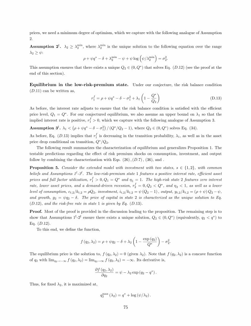
prices, we need a minimum degree of optimism, which we capture with the following analogue of Assumption

2.

Assumption 2I. λ2 ≥ λmin2 , where λmin2 is the unique solution to the following equation over the range

λ2 ≥ ψ:ρ+ ψq∗ − δ + λmin2 − ψ + ψ log

(ψ/λmin2

)= σ22.

This assumption ensures that there exists a unique Q2 ∈ (0, Q∗) that solves Eq. (D.12) (see the proof at the

end of this section).

Equilibrium in the low-risk-premium state. Under our conjecture, the risk balance condition

(D.11) can be written as,

rf1 = ρ+ ψq∗ − δ − σ21 + λ1

(1− Q∗

Q2

)(D.13)

As before, the interest rate adjusts to ensure that the risk balance condition is satisfied with the effi cient

price level, Q1 = Q∗. For our conjectured equilibrium, we also assume an upper bound on λ1 so that the

implied interest rate is positive, rf1 > 0, which we capture with the following analogue of Assumption 3.

Assumption 3I. λ1 <(ρ+ ψq∗ − δ − σ21

)/ (Q∗/Q2 − 1), where Q2 ∈ (0, Q∗) solves Eq. (34).

As before, Eq. (D.13) implies that rf1 is decreasing in the transition probability, λ1, as well as in the asset

price drop conditional on transition, Q∗/Q2.

The following result summarizes the characterization of equilibrium and generalizes Proposition 1. The

testable predictions regarding the effect of risk premium shocks on consumption, investment, and output

follow by combining the characterization with Eqs. (26) , (D.7) , (36), and .

Proposition 5. Consider the extended model with investment with two states, s ∈ {1, 2}, with commonbeliefs and Assumptions 1I-3I . The low-risk-premium state 1 features a positive interest rate, effi cient asset

prices and full factor utilization, rf1 > 0, Q1 = Q∗ and η1 = 1. The high-risk state 2 features zero interest

rate, lower asset prices, and a demand-driven recession, rf2 = 0, Q2 < Q∗, and η2 < 1, as well as a lower

level of consumption, ct,2/kt,2 = ρQ2, investment, it,2/kt,2 = ψ (Q2 − 1) , output, yt,2/kt,2 = (ρ+ ψ)Q2−ψ,and growth, g2 = ψq2 − δ. The price of capital in state 2 is characterized as the unique solution to Eq.

(D.12), and the risk-free rate in state 1 is given by Eq. (D.13).

Proof. Most of the proof is provided in the discussion leading to the proposition. The remaining step is toshow that Assumptions 1I-2I ensure there exists a unique solution, Q2 ∈ (0, Q∗) (equivalently, q2 < q∗) to

Eq. (D.12).

To this end, we define the function,

f (q2, λ2) = ρ+ ψq2 − δ + λ2

(1− exp (q2)

Q∗

)− σ22.

The equilibrium price is the solution to, f (q2, λ2) = 0 (given λ2). Note that f (q2, λ2) is a concave function

of q2 with limq2→−∞ f (q2, λ2) = limq2→∞ f (q2, λ2) = −∞. Its derivative is,

∂f (q2, λ2)

∂q2= ψ − λ2 exp (q2 − q∗) .

Thus, for fixed λ2, it is maximized at,

qmax2 (λ2) = q∗ + log (ψ/λ2) .

75

Moreover, the maximum value is given by

f (qmax2 (λ2) , λ2) = ρ− δ + ψ (q∗ + log (ψ/λ2)) + λ2 (1− exp (log (ψ/λ2)))− σ22= ρ− δ + ψq∗ + ψ log (ψ/λ2) + λ2 − ψ − σ22.

Next note that, by Assumption 1I , the maximum value is strictly negative when λ2 = ψ, that is,

f (qmax2 (ψ) , ψ) < 0. Note also that df(qmax2 (λ2),λ2)dλ2

= 1 − ψλ2, which implies that the maximum value is

strictly increasing in the range λ2 ≥ ψ. Since limλ2→∞ f (qmax2 (λ2) , λ2) = ∞, there exists λmin2 > ψ that

ensures f(qmax2

(λmin2

), λmin2

)= 0. By Assumption 2I , the transition probability satisfies λ2 ≥ λmin2 ,

which implies that f (qmax2 (λ2) , λ2) ≥ 0. By Assumption 1I , we also have that f (q∗, λ2) < 0. It follows

that, under Assumptions 1I-2I , there exists a unique price level, q2 ∈ [qmax2 , q∗), that solves the equation,

f (q2, λ2) = 0.

D.3. New Keynesian microfoundations for nominal rigidities with investment

In the rest of this appendix, we present the microfoundations for nominal rigidities that lead to Eqs. (D.5)

and (D.6). The production structure is the same as in Appendix B.1.2. Specifically, there is a continuum

of monopolistically competitive production firms that produce intermediate goods according to (B.3), and

there is a competitive sector that produces the final good according to (B.4). This also implies the demand

for production firms is given by(B.5). One difference is that production firms do not own the capital but they

rent it from investment firms at rate Rt,s. Hence, they choose how their capital input kt,s (ν), in addition to

their factor utilization rate, ηt,s (ν), as well as production and pricing decisions, yt,s (ν) , pt,s (ν).

These features ensure that the production firm’s output will be split between their capital expenditures

(that they pay to investment firms) and monopoly profits. To simplify the analysis, we make assumptions

so that there are no monopoly profits in equilibrium (and all output accrues to investment firms as return to

capital). Specifically, we assume the government taxes the firm’s profits lump sum, and redistributes these

profits to the firms in the form of a linear subsidy to capital.

Formally, we let Πt,s (ν) denote the equilibrium pre-tax profits of firm ν (that will be characterized

below). We assume each firm is subject to the lump-sum tax determined by the average profits of all firms,

Tt,s =

∫ν

Πt,s (ν) dν. (D.14)

We also let Rt,s − τ t,s denote the after-subsidy cost of renting capital, where Rt,s denotes the equilibriumrental rate paid to investment firms, and τ t,s denotes a linear subsidy paid by the government. We assume

the magnitude of the subsidy is determined by the government’s break-even condition,

τ t,s

∫ν

kt,s (ν) dν = Tt,s. (D.15)

Without price rigidities, the firm chooses pt,s (ν) , kt,s (ν) , ηt,s (ν) ∈ [0, 1] , yt,s (ν) , to maximize its (pre-

tax) profits,

Πt,s (ν) ≡ pt,s (ν) yt,s (ν)− (Rt,s − τ t,s) kt,s (ν) , (D.16)

subject to the supply constraint in (B.3) and the demand constraint in (B.5). As in Appendix B.1.2, the

76

demand constraint holds as equality. Then, the optimality conditions imply,

ηt,s (ν) = 1 and pt,s (ν) =ε

ε− 1

Rt,s − τ t,sA

.

That is, the firm utilizes its capital at full capacity (as before) and it increases its capital input and production

up to the point at which its price is a constant markup over its after-subsidy marginal cost. In a symmetric-

price equilibrium, we further have, pt,s (ν) = 1. Using Eqs. (B.3) and (D.15), this further implies,

yt,s (ν) = yt,s = Akt,s and Rt,s =ε− 1

εA+ τ t,s = A. (D.17)

That is, output is equal to potential output, and capital earns its marginal contribution to potential output

(in view of the linear subsidies).

Now consider the alternative setting in which the firms have a preset nominal price that is equal across

firms, Pt,s (ν) = P . In particular, the relative price of a firm is fixed and equal to one, pt,s (ν) = 1. The firm

chooses the remaining variables, kt,s (ν) , ηt,s (ν) ∈ [0, 1] , yt,s (ν), to maximize its (pre-tax) profits, Πt,s (ν),

subject to the supply constraint in (B.3) and the demand constraint, (B.5). Combining the constraints and

using pt,s (ν) = 1, the firm’s problem can be written as,

maxηt,s(ν),kt,s(ν)

Aηt,s (ν) kt,s (ν)− (Rt,s − τ t,s) kt,s (ν) s.t. 0 ≤ ηt,s (ν) ≤ 1 and Aηt,s (ν) kt,s (ν) ≤ yt,s.

We conjecture an equilibrium in which Rt,s = τ t,s and firms choose symmetric capital inputs, kt,s (ν) = kt,s.

Under this equilibrium, the marginal cost of renting capital is zero, Rt,s − τ t,s = 0. This verifies that it

is optimal for firms to choose symmetric inputs, kt,s (ν) = kt,s. After substituting these expressions, the

firm’s problem becomes equivalent to its counterpart in Appendix B.1.2. Following the same steps there,

the optimal factor utilization is given by ηt,s (ν) =yt,sAkt,s

≤ 1. Hence, output is determined by aggregate

demand, yt,s, subject to the capacity constraint, ηt,s (ν) ≤ 1.

In the conjectured equilibrium, the production firms choose the same level of inputs and factor utilization

rates and produce the same level of output as each other. Therefore, they also have the same level of pre-

tax profits. Using Eqs. (D.16) together with Rt,s = τ t,s = 0, we also calculate the pre-tax profit level as

Πt,s = yt,s. Substituting this into Eqs. (D.14) and (D.15), we obtain τ t,s = yt,s/kt,s = ηt,sA. Substituting

this into Eq. (D.16), we further obtain Rt,s = yt,s/kt,s = ηt,sA. This verifies the conjecture, Rt,s = τ t,s.

In sum, when the firms’nominal prices are fixed, aggregate output is determined by aggregate demand

subject to the capacity constraint, which verifies Eq. (D.5). Moreover, thanks to lump-sum costs to profits

and linear subsidies to capital, all output accrues to the investment firms as return to capital, which verifies

Eq. (D.6).

77

E. Appendix: Data Details and Omitted Empirical Results

This appendix presents the details of the data sources and variable construction used in Section 7, and

presents the empirical results (tables and figures) omitted from the main text.

House price index. We rely on the cross-country quarterly panel dataset described in Mack et al. (2011).The dataset is regularly updated and publicly available at https://www.dallasfed.org/institute/houseprice.

We use the inflation-adjusted (real) house price index measure to construct the shock variable in our re-

gression analysis (see (54)). Our country coverage is to a large extent determined by the availability of this

measure, e.g., we exclude a few developed countries such as Portugal and Austria for which we do not have

consistent data on real house prices.

Euro or Exchange Rate Mechanism (Euro/ERM) status. We hand-collect this data from various

online sources. A country-quarter is included in the Euro/ERM sample if the country is a member of the

Euro or the European Exchange Rate mechanism in most of the corresponding calendar year. Table 1

describes the Euro/ERM status by year for all countries in our sample.

GDP, consumption, investment. We obtain this data from the OECD’s quarterly national accounts

dataset (available at https://stats.oecd.org). We use the variables calculated according to the expenditure

approach. The corresponding OECD subject codes are as follows:

• GDP: “B1_GE”(Gross domestic product —expenditure approach).

• Consumption: “P31S14_S15”(Private final consumption expenditure)

• Investment: “P51”(Gross fixed capital formation)

For each of these variables, we use the measures that are adjusted for inflation as well as seasonality. The

OECD measure code is: “LNBQRSA”(National currency, chained volume estimates, national reference year,

quarterly levels, seasonally adjusted).

Relative GDP (with PPP-adjusted prices in a common base year). We obtain an alternative

GDP measure from the OECD’s annual national accounts dataset (available at https://stats.oecd.org). We

use the variable calculated according to the expenditure approach (with subject code “B1_GE”), measured

with PPP-adjusted prices in a common base year. The OECD measure code is: “VPVOB”(Current prices,

constant PPPs, OECD base year). We use the value of this measure in 1990 to weight all of our regressions

(see (54)).

CPI. We obtain this data from the OECD’s prices and purchasing power parities dataset (available at

https://stats.oecd.org). We use the core CPI measure that excludes food and energy. The OECD subject

code is: “CPGRLE”(Consumer prices - all items non-food, non-energy). We use the annual measure, which

is less subject to seasonality, and we linearly interpolate this to obtain a quarterly measure.

Unemployment rate. We obtain this data from the OECD’s key short-term economic indicators database(available at https://stats.oecd.org). We use the harmonized unemployment rate measure with seasonal ad-

justment and at quarterly frequency. The OECD subject code is “LRHUTTTT”(Harmonised unemployment

rate: all persons, s.a).

78

The policy interest rate. Obtaining the policy interest rate is not as trivial as it might sound since differentcentral banks conduct monetary policy in terms of different target rates (and sometimes without specifying

a target rate, or by monitoring multiple rates). On the other hand, the selection does not substantially

affect the results since short-term risk-free rates within a developed country are often highly correlated.

Following Romer and Romer (2018), we use announced policy target rates when available, and otherwise we

use collateralized short-term market rates (such as Repo rates or Lombard rates). For Eurozone countries,

we use the local collateralized rate until the country joins the Euro, and we switch to the European Central

Bank’s (ECB) main refinancing operations (MRO) rate after the country joins the Euro.

For most of the countries, we construct our own measure of the policy interest rate according to

the above selection criteria by using data from the Global Financial Data’s GFDATABASE (GFD).

This is a proprietary database that contains a wealth of information on various asset prices (see

https://www.globalfinancialdata.com for details).

For a few countries (specified below), we instead rely on the Bank for International

Settlements’s (BIS) database on central bank policy interest rates (publicly available at

https://www.bis.org/statistics/cbpol.htm). We switch to the BIS measure when we cannot construct

an appropriate measure using the GFD; or when the BIS measure has greater coverage than ours and the

two measures are highly correlated. From either database, we obtain monthly data and convert to quarterly

data by averaging over the months within the quarter.

• United States: GFD ticker “IDUSAFFD”(USA Fed Funds Offi cial Target Rate).

• United Kingdom: GFD ticker “IDGBRD”(Bank of England Base Lending Rate).

• Australia: GFD ticker “IDAUSD”(Australia Reserve Bank Overnight Cash Rate).

• South Korea: GFD ticker “IDKORM”(Bank of Korea Discount Rate).

• Germany: GFD ticker “IDDEULD” (Germany Bundesbank Lombard Rate) until the country joins

the Euro. Afterwards, we use the ECB MRO rate. The corresponding GFD ticker is: “IDEURMW”

(Europe Marginal Rate on Refinancing Operations).

• New Zealand: GFD ticker “IDNZLD”(New Zealand Reserve Bank Offi cial Cash Rate).

• France: GFD ticker “IDFRARD”(Bank of France Repo Rate) until the country joins the Euro.

• Denmark: We use the BIS measure (highly correlated with our measure and greater coverage).

• Finland: GFD ticker “IDFINRM”(Bank of Finland Repo Rate) until the country joins the Euro.

• Sweden: GFD ticker “IDSWERD”(Sweden Riksbank Repo Rate).

• Israel: GFD ticker “IDISRD”(Bank of Israel Discount Rate).

• Italy: GFD ticker “IDITARM”(Bank of Italy Repo Rate) until the country joins the Euro.

• Spain: GFD ticker “IDESPRM”(Bank of Spain Repo Rate) until the country joins the Euro.

• Ireland: GFD ticker “IDIRLRD”(Bank of Ireland Repo Rate) until the country joins the Euro.

• Belgium: GFD ticker “IDBELRM”(Belgium National Bank Repo Rate) until the country joins the

Euro.

• Greece: GFD ticker “IDGRC”D (Bank of Greece Discount Rate) until the country joins the Euro.

79

• Netherlands: GFD ticker “IDNLDRD” (Netherlands Bank Repo Rate) until the country joins the

Euro.

• Norway: GFD ticker “IDNORRD”(Bank of Norway Sight Deposit Rate).

• Japan: GFD ticker “IDJPNCM”(Japan Target Call Rate). GFD data is missing from March 2001

until July 2006. BIS data is also missing for most of this period. We use other sources to hand-fill the

interest rate over this period as being equal to 0% (see for instance, the data from St. Louis Fed at

https://fred.stlouisfed.org/series/IRSTCI01JPM156N).

• Switzerland: We use the BIS measure (cannot identify an appropriate rate from the GFD).

• Canada: We use the BIS measure (highly correlated with our measure and greater coverage).

Stock prices. We obtain this data from the GFD. For each country, we try to pick the most popular stock

price index (based on Internet searches). We obtain daily data and convert to quarterly data by averaging

over all (trading) days within the quarter. We then divide this with our core CPI measure (see above) to

obtain a real stock price series.

• United States: GFD ticker “_SPXD”(S&P500 Index)

• United Kingdom: GFD ticker “_FTSED”(UK FTSE100 Index).

• Australia: GFD ticker “_AXJOD”(Australia S&P/ASX 200 Index).

• South Korea: GFD ticker “_KS11D”(Korea SE Stock Price Index (KOSPI)).

• Germany: GFD ticker “_GDAXIPD”(Germany DAX Price Index).

• New Zealand: GFD ticker “_NZ15D”(NZSX-15 Index).

• France: GFD ticker “_FCHID”(Paris CAC-40 Index).

• Denmark: GFD ticker “_OMXC20D”(OMX Copenhagen-20 Index).

• Finland: GFD ticker “_OMXH25D”(OMX Helsinki-25 Index).

• Sweden: GFD ticker “_OMXS30D”(OMX Stockholm-30 Index).

• Israel: GFD ticker “_TA125D”(Tel Aviv SE 125 Broad Index).

• Italy: GFD ticker “_BCIJD”(Milan SE MIB-30 Index).

• Spain: GFD ticker “_IBEXD”(Madrid SE IBEX-35 Index).

• Ireland: GFD ticker “_ISEQD”(Ireland ISEQ Overall Price Index).

• Belgium: GFD ticker “_BFXD”(Belgium CBB Bel-20 Index).

• Greece: GFD ticker “_ATGD”(Athens SE General Index).

• Netherlands: GFD ticker “_AEXD”(Amsterdam AEX Stock Index).

• Norway: GFD ticker “_OSEAXD”(Oslo SE All-Share Index).

• Japan: GFD ticker “_N225D”(Nikkei 225 Stock Index).

• Switzerland: GFD ticker “_SSMID”(Swiss Market Index).

80

• Canada: GFD ticker “_GSPTSED”(Canada S&P/TSX 300 Index).

Earnings. We obtain monthly data on the price-earnings ratio of publicly traded firms from the GFD

(typically constructed for a broad sample of stocks chosen by the GFD). We then combine this information

with our nominal price index (using the price at the last trading day of the month) to construct a monthly

series for earnings. We convert this to a quarterly measure by averaging over the months within the quarter.

We then divide this by our core CPI measure to obtain a quarterly real earnings series for publicly traded

firms.

GFD ticker for the price earnings ratio typically has the form “SY-three digit country code-PM”(e.g.,

the ticker for the United States is “SYUSAPM”). One exception is the United Kingdom for which the

corresponding GFD code is “_PFTASD”(UK FT-Actuaries PE Ratio).

Credit expansion. Our measure of bank credit is based on Baron and Xiong (2017), who construct a

variable, credit expansion, defined as the annualized past three-year change in bank credit to GDP ratio.

Mathematically, it is expressed as

credit expansion =∆(bank creditGDP

)t−∆

(bank creditGDP

)t−12

12× 4, (E.1)

where t denotes a quarter. Baron and Xiong (2017) construct this measure by merging data from two sources.

Their main source is the “bank credit”measure from the BIS, which covers a large set of countries but is

generally available only for postwar years. For this reason, Baron and Xiong (2017) also supplement it with

the “bank loans”measure from Schularick and Taylor (2012), which covers fewer countries but more years.

Since our panel starts in 1990, we ignore the second source and rely entirely on the BIS measure.

Specifically, we use the quarterly BIS database on credit to the nonfinancial sector (publicly available at

https://www.bis.org/statistics/totcredit.htm). We obtain the measure “bank credit to the private nonfinan-

cial sector”expressed in units of percentage of GDP (the corresponding BIS code is “Q:5A:P:B:M:770:A”),

which enables us to construct the variable in (E.1). We verify that our variable is highly correlated with the

measure constructed by Baron and Xiong (2017) (who generously shared their data with us)– the correlation

coeffi cient for the available country-quarters is 0.975.

Following Baron and Xiong (2017), we also construct a “credit expansion-std”variable by standardizing

the measure in (E.1) by its mean and standard deviation within each country. Since Baron and Xiong (2017)

focus on predicting stock prices, they calculate the mean and the standard deviation using only past data

so as to avoid any look-ahead bias. Since our focus is different, we ignore this subtlety and calculate the

sample statistics using the entire data for the corresponding country (in the BIS database).

81

Table 1: Euro/ERM status by country and yearCountry 1990 1991 1992 1993 1994 1995 1996 1997-2017

Belgium 1 1 1 1 1 1 1 1Denmark 1 1 1 1 1 1 1 1Finland 0 0 0 0 0 0 0 1France 1 1 1 1 1 1 1 1Germany 1 1 1 1 1 1 1 1Greece 0 0 0 0 0 0 1 1Ireland 1 1 1 1 1 1 1 1Italy 1 1 1 0 0 0 0 1

Netherlands 1 1 1 1 1 1 1 1Spain 1 1 1 1 1 1 1 1

Australia 0 0 0 0 0 0 0 0Canada 0 0 0 0 0 0 0 0Israel 0 0 0 0 0 0 0 0Japan 0 0 0 0 0 0 0 0Korea 0 0 0 0 0 0 0 0NZL 0 0 0 0 0 0 0 0Norway 0 0 0 0 0 0 0 0Sweden 0 1 1 0 0 0 0 0

Switzerland 0 0 0 0 0 0 0 0UK 0 1 1 0 0 0 0 0USA 0 0 0 0 0 0 0 0

Euro status. Belgium, Finland, France, Germany, Ireland, Italy, Netherlands, Spain adopted the Euro in1999. Greece adopted in 2001. Denmark hasn’t adopted the Euro but is a member of the ERM.

82

Table 2: Summary statistics by ERM for the baseline regression sampleERM sample Non-ERM sample Difference

Mean Std.Deviation Mean Std.Deviation Mean Std.Error∆ log house prices (real) 0.0040 0.0183 0.0053 0.0181 -0.0013 (0.0023)

∆ log GDP (real) 0.0043 0.0128 0.0065 0.0093 -0.0022 (0.0010)

policy interest rate (nominal) 0.0232 0.0194 0.0352 0.0288 -0.0119 (0.0038)

∆ log CPI (core) 0.0041 0.0029 0.0046 0.0039 -0.0004 (0.0005)

∆ unemployment rate -0.0000 0.0042 -0.0002 0.0030 0.0002 (0.0004)

∆ log investment (real) 0.0030 0.0535 0.0070 0.0297 -0.0040 (0.0021)

∆ log consumption (real) 0.0035 0.0103 0.0069 0.0095 -0.0034 (0.0008)

earnings to price ratio 0.0616 0.0409 0.0585 0.0227 0.0031 (0.0039)

∆ log stock prices (real) 0.0011 0.0974 0.0108 0.0820 -0.0097 (0.0047)

credit expansion 0.0175 0.0557 0.0136 0.0298 0.0040 (0.0079)

credit expansion-std 0.1715 1.2657 -0.0346 1.1128 0.2062 (0.1957)Observations 821 1120 1941

∆ represents quarterly change. Standard errors are Newey-West standard errors with a bandwidth of 20 quarters.

83

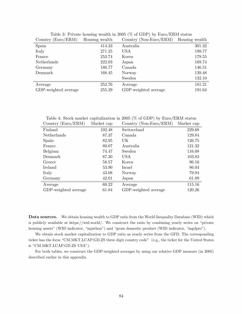
Table 3: Private housing wealth in 2005 (% of GDP) by Euro/ERM statusCountry (Euro/ERM) Housing wealth Country (Non-Euro/ERM) Housing wealth

Spain 414.33 Australia 301.32Italy 271.25 USA 199.77France 253.74 Korea 179.55Netherlands 222.03 Japan 169.74Germany 186.77 Canada 146.51Denmark 168.45 Norway 139.48

Sweden 132.10

Average 252.76 Average 181.21GDP-weighted average 255.29 GDP-weighted average 191.64

Table 4: Stock market capitalization in 2005 (% of GDP) by Euro/ERM statusCountry (Euro/ERM) Market cap Country (Non-Euro/ERM) Market cap

Finland 102.48 Switzerland 229.68Netherlands 87.37 Canada 129.84Spain 82.95 UK 126.75France 80.07 Australia 121.32Belgium 74.47 Sweden 116.08Denmark 67.30 USA 103.83Greece 58.57 Korea 96.16Ireland 53.90 Israel 86.04Italy 43.08 Norway 79.94Germany 42.01 Japan 61.89

Average 69.22 Average 115.16GDP-weighted average 61.84 GDP-weighted average 120.26

Data sources. We obtain housing wealth to GDP ratio from the World Inequality Database (WID) which

is publicly available at https://wid.world/. We construct the ratio by combining yearly series on “private

housing assets”(WID indicator, “mpwhou”) and “gross domestic product (WID indicator, “mgdpro”).

We obtain stock market capitalization to GDP ratio as yearly series from the GFD. The corresponding

ticker has the form “CM.MKT.LCAP.GD.ZS three digit country code” (e.g., the ticker for the United States

is “CM.MKT.LCAP.GD.ZS USA”).

For both tables, we construct the GDP-weighted averages by using our relative GDP measure (in 2005)

described earlier in this appendix.

84

0.1

.2.3

0 4 8 12

policy interest rate (pp)­.3

­.1.1

0 4 8 12

core cpi (percent)

­.1.3

.7

0 4 8 12

unemployment rate (pp)

­.9­.3

.3

0 4 8 12

GDP (percent)

­3­1

.2.6

0 4 8 12

investment (percent)

­.7­.2

.3

0 4 8 12

consumption (percent)

­.5­.2

.1

0 4 8 12

earnings/initial price (pp)

­4.1

­1.7

.7

0 4 8 12

stock prices (percent)

­2.6

­1.1

.4

0 4 8 12

house prices (percent)

Impulse responses to 1 percent decrease in real house prices (Euro/ERM minus Non­Euro/ERM)

Figure 10: Differences in coeffi cients between the ERM and the non-ERM samples correspondingto the baseline regression results in Figure 6.

85

­.2­.1

0

0 4 8 12

policy interest rate (pp)­.2

0

0 4 8 12

core cpi (percent)

0.2

.4

0 4 8 12

unemployment rate (pp)

­.6­.2

.2

0 4 8 12

GDP (percent)

­2­.9

.2

0 4 8 12

investment (percent)

­.9­.4

.1

0 4 8 12

consumption (percent)

­.2.1

.4

0 4 8 12

earnings/initial price (pp)

­2.4

­.71

0 4 8 12

stock prices (percent)

­1.1

01.

1

0 4 8 12

house prices (percent)

Additional impulse responses to 1 percent decrease in real house prices (Euro/ERM minus Non­Euro/ERM)when credit expansion has been one standard dev iation abov e average

Figure 11: Differences in coeffi cients between the ERM and the non-ERM samples correspondingto the regression results with credit interaction in Figure 7.

86

­.4­.1

.2

0 4 8 12

policy interest rate (pp)­.1

.1

0 4 8 12

core cpi (percent)

0.5

1

0 4 8 12

unemployment rate (pp)

­1.3

­.6.1

0 4 8 12

GDP (percent)

­4.2

­2.1

0

0 4 8 12

investment (percent)

­1.2

­.60

0 4 8 12

consumption (percent)

­.6­.2

.2

0 4 8 12

earnings/initial price (pp)

­5.2

­1.3

2.6

0 4 8 12

stock prices (percent)

­6­3

0

0 4 8 12

house prices (percent)

Impulse responses to 1 percent decrease in real house prices (without time f ixed ef f ects)

 Euro/ERM  Non­Euro/ERM

Figure 12: The analogues of the baseline regression results in Figure 6 with the difference that timefixed effects are excluded from the regressions.

87

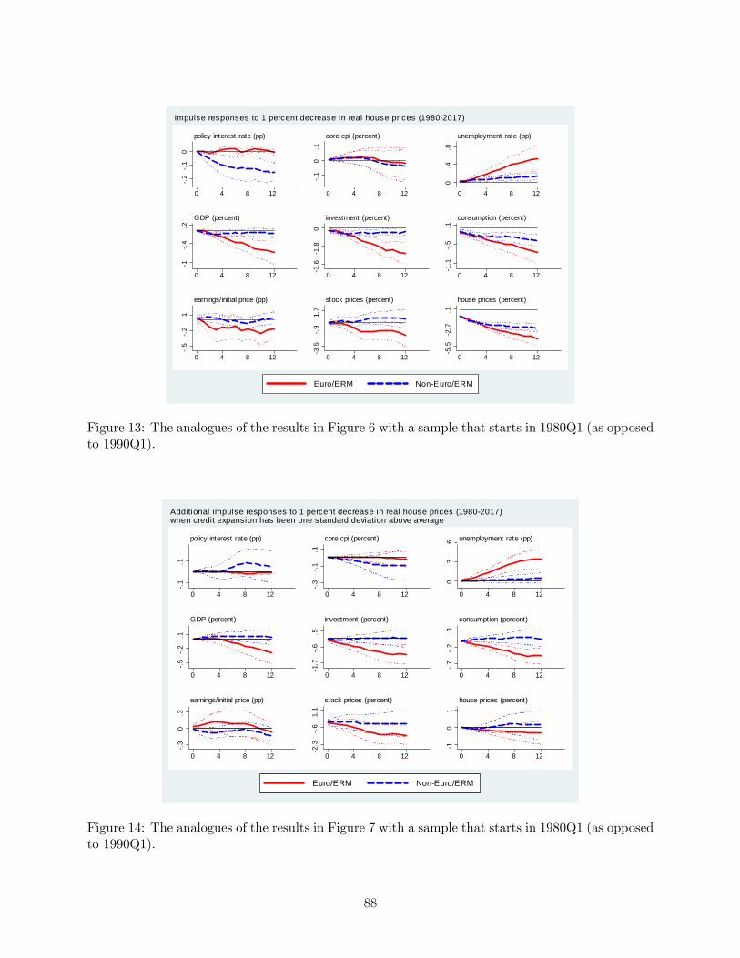
­.2

­.1

00 4 8 12

policy interest rate (pp)

­.1

0.1

0 4 8 12

core cpi (percent)

0.4

.8

0 4 8 12

unemployment rate (pp)

­1­.

4.2

0 4 8 12

GDP (percent)

­3.6

­1.8

0

0 4 8 12

investment (percent)

­1.1

­.5

.1

0 4 8 12

consumption (percent)

­.5

­.2

.1

0 4 8 12

earnings/initial price (pp)

­3.5

­.9

1.7

0 4 8 12

stock prices (percent)

­5.5

­2.7

.1

0 4 8 12

house prices (percent)

Impulse responses to 1 percent decrease in real house prices (1980­2017)

 Euro/ERM  Non­Euro/ERM

Figure 13: The analogues of the results in Figure 6 with a sample that starts in 1980Q1 (as opposedto 1990Q1).

­.1

.1

0 4 8 12

policy interest rate (pp)

­.3

­.1

.1

0 4 8 12

core cpi (percent)

0.3

.6

0 4 8 12

unemployment rate (pp)

­.5

­.2

.1

0 4 8 12

GDP (percent)

­1.7

­.6

.5

0 4 8 12

investment (percent)

­.7

­.2

.3

0 4 8 12

consumption (percent)

­.3

0.3

0 4 8 12

earnings/initial price (pp)

­2.3

­.6

1.1

0 4 8 12

stock prices (percent)

­10

1

0 4 8 12

house prices (percent)

Additional impulse responses to 1 percent decrease in real house prices (1980­2017)when credit expansion has been one standard deviation above average

 Euro/ERM  Non­Euro/ERM

Figure 14: The analogues of the results in Figure 7 with a sample that starts in 1980Q1 (as opposedto 1990Q1).

88

­6­2

.9.2

0 4 8 12

house prices (percent)

­7.1

­1.6

3.9

0 4 8 12

stock prices (percent)

Impulse responses to 1 percentage point increase in policy interest rate (full sample)

Figure 15: The analogues of the baseline regression results in Figure 6, where we consider shocksto the policy interest rate as opposed to house prices. Specifically, we run the analogue of thespecification in (54) (on the full sample) where the shock variable is the level of the policy interestrate and the outcome variable is log house prices (left panel) or log stock prices (right panel).The solid lines plot the coeffi cients corresponding to the the policy interest rate variable. Allregressions include time and country fixed effects; 12 lags of the level of the policy interest rate,contemporaneous value and 12 lags of the first difference of log GDP, 12 lags of the first differenceof log house prices, and 12 lags of the first difference of log stock prices. The dotted lines show95% confidence intervals calculated according to Newey-West standard errors with a bandwidthof 20 quarters. All regressions are weighted by countries’PPP-adjusted GDP in 1990. Data isunbalanced quarterly panel that spans 1990Q1-2017Q4. All variables except for the policy interestrate are adjusted for inflation. The sources and the definitions of variables are described earlier inthis appendix.

89