A Risk-centric Model of Demand Recessions and

Macroprudential Policy

Ricardo J. Caballero and Alp Simsek∗

This draft: July 14, 2017

Abstract

A productive capacity generates output and risks, both of which need to be absorbed

by economic agents. If they are unable to do so, output and risk gaps emerge. Risk gaps

close quickly: A decline in the interest rate increases the Sharpe ratio of the risky assets and

equilibrates the risk markets. If the interest rate is constrained from below (or the policy

response is slow), the risk markets are instead equilibrated via a decline in asset prices.

However, the drop in asset prices also drags down aggregate demand, which further drags

prices down, and so on. If economic agents are optimistic about the speed of recovery, a

decline in asset prices leads to a large increase in the Sharpe ratio that stabilizes the drop.

If they are pessimistic, the economy becomes highly susceptible to downward spirals due to

the feedback between asset prices and aggregate demand. When beliefs are heterogenous,

optimists take too much risk from a social point of view since they do not internalize their

positive effect on asset prices and aggregate demand during recessions. Macroprudential

policy can improve outcomes, and is procyclical as the negative aggregate demand effect of

prudential tightening is more easily offset by interest rate policy during booms than during

recessions. Forward guidance policies are also effective, but their robustness weakens as

agents become more pessimistic. Our model also illustrates that interest rate rigidities and

speculation generate endogenous price volatility that exacerbates demand recessions.

JEL Codes: E00, E12, E21, E22, E30, E40, G00, G01, G11Keywords: Risk-gap, output-gap, aggregate demand, aggregate supply, liquidity trap, in-

terest rates, “rstar,”portfolio decisions, Sharpe ratio, monetary and macroprudential policy,

forward guidance, heterogeneous beliefs, speculation, tail risk, endogenous volatility.

∗MIT and NBER. Contact information: caball@mit.edu and asimsek@mit.edu. We thank Emmanuel Farhi,Zhiguo He, Zilu Pan, Matthew Rognlie, Olivier Wang, Nathan Zorzi, and participants at the CCBS conferencehosted by the Bank of England and MacCalm, Paris School of Economics, and BIS, for their comments. Simsekacknowledges support from the National Science Foundation (NSF) under Grant Number SES-1455319. Firstdraft: May 11, 2017

1

02

46

8E

quity

 risk

 pre

miu

m (%

, one

 yea

r ahe

ad)

1990 1995 2000 2005 2010 2015time

US average of G5

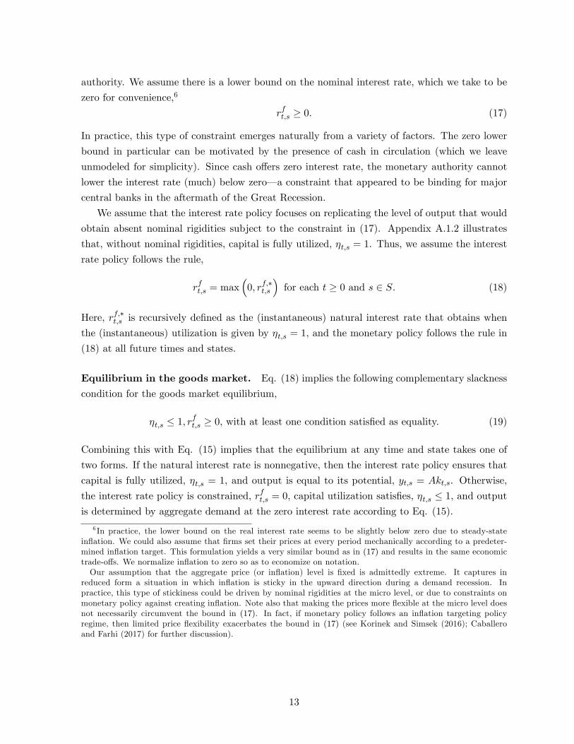
Figure 1: Solid line plots the (forward looking) equity risk premium for the US. Dashed lineplots the unweighted average premium for the G5 countries (the US, Japan, the UK, Germany,France). Source: Constructed by Datastream as the median of nine different methods to calculatethe ERP. Mean-based methods tend to give higher levels but similar shapes for the path of theERP.

1. Introduction

A productive capacity generates output and risks, both of which need to be absorbed by economic

agents. If they are unwilling or unable to do so, output- and risk-gaps emerge that require

appropriate policy responses to prevent severe downward spirals. Macroeconomic modeling has

focused primarily on the output-gap component, however risk considerations are central for

private and policy decisions, and have become even more prominent since the subprime crisis.

Figure 1 shows an estimate of the path of the expected equity risk premium (ERP) for the U.S.

and the average of the G5 countries. Several risk-intolerance patterns are apparent in this figure:

(i) the ERP spiked during the subprime and European crises; (ii) the ERP remained elevated

through much of the U.S. recovery; and (iii) at the global level there is little evidence that the

ERP will go to pre-crisis levels any time soon. Our main goal in this paper is to provide a

dynamic macroeconomic model that highlights the role of risk markets equilibrium in business

cycles (hence the “risk-centric”in the title).

We develop a continuous time macrofinance model with aggregate demand channels and

2

speculative motives due to heterogeneous beliefs.1 In this model, shocks interact with interest

rate policy and its constraints in determining the output gap and the natural interest rate

(“rstar”). Also, while the degree of optimism of economic agents is key in containing the fall

during recessions, optimists’risk taking is potentially destabilizing, which generates a role for

macroprudential policy.

The supply side of the (model-)economy is a stochastic AK model with capital-adjustment

costs and sticky prices. The demand side has standard risk-averse consumer-investors that

demand the goods and risky assets. In equilibrium, the volatility of their consumption is equal

to “the Sharpe ratio”of capital (a measure of the risk-adjusted expected return in excess of the

risk-free rate). Our analysis rests on the mechanism by which this risk condition is achieved.

Economic agents only differ (when they do) in their beliefs with respect to the likelihood of a

near-term recession or recovery. There are no financial frictions in the main environment (we

introduce them in the last section). Instead, we focus on “interest-rate frictions”: factors that

might constrain or delay the adjustment of the risk-free interest rate to shocks. For concreteness,

we work with a zero lower bound on the interest rate.

The model has productivity and volatility shocks; we view the latter as capturing a variety

of factors that affect the risk premium. In the absence of interest-rate frictions, it is “rstar”that

absorbs these types of shocks. The natural interest rate ensures that output is determined by

the supply side of the economy. By Walras law, this also implies that there is no risk gap, as the

desired volatility of consumption exactly matches the assets’fundamental volatility generated

by the productive capacity of the economy. That is, when viewed from the perspective of risk

markets, “rstar”ensures that the perceived Sharpe ratio of the returns of the fully utilized stock

of capital is consistent with investor’s desired risk holdings. It follows that “rstar”is not only a

function of goods-markets but also of risk-markets conditions.

To fix ideas, consider a shock that increases volatility. The immediate effect of this shock

is to decrease the Sharpe ratio of capital. A risk gap develops, in the sense that the economy

generates too much risk relative to what investors are willing to absorb. The natural response

of the economy is a decrease in the interest rate, which increases the Sharpe ratio and restores

equilibrium in risk markets (as well as goods markets).

If there is a lower bound on the interest rate, the economy loses its natural line of defense.

Instead, the risk markets are equilibrated via a decline in asset prices, which increases the

Sharpe ratio via expected capital gains. However, the wealth and investment effects of such

price adjustment implies that the goods market becomes demand constrained and the economy

experiences excess capacity, which further reduces asset prices, which again feeds into aggregate

1By a macrofinance model we mean, following (and quoting) Brunnermeier and Sannikov (2016b): “Instead offocusing only on levels, the first moments, the second moments, and movements in risk variables are all an integralpart of the analysis, as they drive agents’consumption, (precautionary) savings and investment decisions.”Also, while in our model heterogenous beliefs have a specific formulation, we intend to capture common features,

especially on the positive analysis, of many mechanisms that generate effective heterogeneity in asset valuation.

3

demand, and so on.

The severity of the recession following the drop in asset prices depends on the relative strength

of the Sharpe and aggregate demand channels. If agents think of the decline in asset prices as

largely temporary, then their perceived Sharpe ratio will rise quickly with a decline in current

asset prices, so only a limited asset price drop is required to restore equilibrium, and hence

the drop in aggregate demand will be mild. Conversely, if agents interpret the decline in asset

prices as a lasting one, then it will take a large drop in asset prices to restore equilibrium in

risk markets, and hence the feedbacks and drop in aggregate demand will be severe. Thus, the

degree of optimism is a critical state variable in our economy, regardless of whether economic

agents have homogeneous or heterogeneous beliefs.

With heterogeneous beliefs, which we analyze in the second part of the paper, the economy’s

degree of optimism depends on the share of wealth in the hands of optimistic and pessimistic

investors. The value of rich optimists for the economy as a whole is high during recessions

since they raise asset valuations, which in turn increases aggregate demand. However there is

nothing in the economy that ensures this allocation of wealth. Differences in beliefs also lead to

speculation which may introduce undesirable correlations between the state of the economy and

the relative wealth of optimists and pessimists. For example, if the main source of discrepancy

during a boom is in the likelihood of a near-term recession, optimists will sell put options which

will impoverish them precisely in the state of the economy that needs them the most. Or, if

during a recession the main source of discrepancy is about the speed of recovery, they will buy

call options which will deplete their wealth if the recession lingers. That is, through relative

wealth effects the economy becomes extrapolative: booms breed optimism and recessions breed

pessimism. Moreover, for any given level of average optimism, as the dispersion of beliefs rises

the anticipation of this extrapolative feature exacerbates the depth of the drop in asset prices

and recession.

Our model generates scope for macroprudential policy, because optimists’(or more broadly,

high-valuation investors’) risk taking is associated with aggregate demand externalities. The

depletion of optimists’wealth during a recession depresses asset prices and aggregate demand.

Optimists do not internalize the effect of their portfolio risks on asset valuations (in subsequent

periods), which leads to excessive risk taking from an aggregate point of view. We show that

making optimistic agents behave as-if they were more pessimistic can lead to a Pareto improve-

ment (that is, we evaluate investors’welfare according to their own beliefs). Moreover, the

policy is naturally procyclical as the tightening of prudential regulation always depresses aggre-

gate demand (in the current period), but this effect can be easily offset with interest rate policy

during booms but not during severe recessions.

Forward guidance is also effective in our model, even when investors have homogeneous

beliefs, since it affects the market’s Sharpe ratio. A decline in future interest rates increases

future asset prices, which increases the expected capital gains. These capital gains translate into

a greater Sharpe ratio, and ultimately, greater asset valuations and aggregate demand. Perhaps

4

surprisingly, forward guidance can be effective even if investors are very pessimistic about the

likelihood of a near term recovery– a manifestation of the “forward guidance puzzle” in our

framework. However, the effectiveness of forward guidance in this case is rather delicate as it

relies on investors’understanding that the forward guidance would continue to stimulate the

economy if the recession persists. In contrast, when investors are optimistic about a near-term

recovery, forward guidance is a more robust policy in the sense that it continues to increase asset

prices even if the policy is transient (or is perceived to be transient). In this sense, our results

are related to a recent strand of the literature illustrating that forward guidance becomes weaker

under informational or behavioral frictions that mitigate the effect of the policy in future periods

(see, for instance, Gabaix (2017), Angeletos and Lian (2016), Farhi and Werning (2016a)).

While we emphasize the effect of exogenous risk shocks– such as changes in volatility or

optimism– on macroeconomic outcomes, the model also generates endogenous price volatility

that creates further amplification. Without interest rate rigidities, the interest rate policy opti-

mally mitigates the impact of risk shocks on asset prices. When the interest rate is constrained,

these shocks translate into price volatility. With heterogeneous beliefs, speculation exacerbates

endogenous price volatility further by creating fluctuations in investors’wealth shares. These

effects are already present in our main model without financial frictions, but they become par-

ticularly salient when we introduce financial frictions. For instance, with incomplete financial

markets, optimists take leveraged positions on capital, and their (relative) net worth becomes ex-

posed to plain-vanilla cyclical (productivity) shocks. The resulting changes in optimists’wealth

share translate into endogenous fluctuations in asset prices as well as aggregate output. In recent

work, Brunnermeier and Sannikov (2014) also obtain endogenous price volatility under a slightly

different set of assumptions, but our model makes the additional prediction that volatility will

be higher when the interest rate policy is constrained. This prediction lends support to the many

unconventional tools aimed at reducing downward volatility, which the major central banks put

in place once interest-rate policy was no longer available during the Great Recession.

Literature review. At a methodological level, our paper belongs in the new continuous time

macrofinance literature started by the seminal work of Brunnermeier and Sannikov (2014, 2016a)

and summarized in Brunnermeier and Sannikov (2016b) (see also Basak and Cuoco (1998);

Adrian and Boyarchenko (2012); He and Krishnamurthy (2012, 2013); Di Tella (2012); Moreira

and Savov (2017); Silva (2016)). This literature seeks to highlight the full macroeconomic

dynamics induced by financial frictions, which force the reallocation of resources from high-

productivity borrowers to low-productivity lenders after a sequence of negative shocks. While

the structure of our economy shares many similarities with theirs, in our main model there are

no financial frictions, and the macroeconomic dynamics stem not from the supply side (relative

productivity) but from the aggregate demand side.

Our paper is also related to an extensive New Keynesian literature that emphasizes the role of

financial frictions and nominal rigidities in driving business cycle fluctuations (see, for instance,

5

Bernanke et al. (1999); Curdia and Woodford (2010); Gertler and Karadi (2011); Gilchrist and

Zakrajšek (2012); Christiano et al. (2014)). Like this literature, we focus on episodes with

high risk premia, but we generate these episodes from changes in risk (or risk perceptions) as

opposed to financial frictions. We also emphasize the role of beliefs (optimism/pessimism) as

well as speculation in exacerbating risk-driven business cycles.

A strand of the literature emphasizes the role of “risk shocks”in exacerbating financial fric-

tions (see, for instance, Christiano et al. (2014); Di Tella (2012)). We share with this literature

the emphasis on uncertainty, but we focus on changes in aggregate risk– as opposed to idiosyn-

cratic uncertainty– which increases risk premia even in absence of frictions. More broadly, there

is an extensive recent empirical literature documenting the importance of uncertainty shocks in

causing and worsening recessions (see, for instance, Bloom (2009)).

The interactions between risk shocks and interest rate lower bounds is also a central theme

of the literature on safe asset shortages and safety traps (see, for instance, Caballero and Farhi

(2017); Caballero et al. (2017b)). We extend this literature by analyzing recurrent business

cycles with multiple shocks, speculation, as well as integrated interest-rate and macroprudential

policies. In recent work, Del Negro et al. (2017) provide a comprehensive empirical evaluation

of the different mechanisms that have put downward pressure on interest rate and argue con-

vincingly that risk and liquidity considerations played a central role (see also Caballero et al.

(2017a)). More broadly, the literature on liquidity traps is extensive and has been rekindled by

the Great Recession (see, for instance, Tobin (1975); Krugman (1998); Eggertsson and Woodford

(2006); Eggertsson and Krugman (2012); Guerrieri and Lorenzoni (2017); Werning (2012); Hall

(2011); Christiano et al. (2015); Eggertsson et al. (2017); Rognlie et al. (2017); Midrigan et al.

(2016); Bacchetta et al. (2016)). We extend this literature by focusing on the risk aspects (both

shocks and mechanisms) behind the drop in the natural rate below its lower bound, as well as

on the interaction between speculation and the severity of recessions.

Our results on macroprudential policy are related to a recent literature that analyzes the

implications of aggregate demand externalities for the optimal regulation of financial markets.

For instance, Korinek and Simsek (2016) show that, in the run-up to deleveraging episodes that

coincide with a zero-lower-bound on the interest rate, welfare can be improved by policies tar-

geted toward reducing household leverage. In Farhi and Werning (2017), the key constraint is

instead a fixed exchange rate, and the aggregate demand externality calls for ex-ante regulation

but also ex-post redistribution, in the form of a fiscal union. In these papers, heterogeneity

in agents’marginal propensities to consume (MPC) is the key determinant of optimal macro-

prudential policy. The policy works by reallocating wealth across agents and states in a way

that high-MPC agents hold relatively more wealth when the economy is more depressed due to

deficient demand. The mechanism in our paper is different and works through heterogeneous

asset valuations. In fact, we work with a log-utility setting in which all agents have the same

marginal propensity to consume. The policy operates by transferring wealth to optimists during

recessions, not because optimists spend more than other agents, but because they raise the asset

6

valuations and induce all investors to spend more (while also increasing aggregate investment).2

Beyond aggregate demand externalities, the macroprudential literature is also extensive,

and mostly motivated by the presence of pecuniary externalities that make the competitive

equilibrium constrained ineffi cient (e.g., Caballero and Krishnamurthy (2003); Lorenzoni (2008);

Bianchi and Mendoza (2013); Jeanne and Korinek (2010)). The friction in this case is not

“nominal” rigidities, but market incompleteness or collateral constraints that depend on asset

prices (see Davila and Korinek (2016) for a detailed exposition). Macroprudential policy typically

improves outcomes by mitigating fire sales that exacerbate financial frictions. The policy in our

model also operates through asset prices but through a different channel. We show that a decline

in asset prices is damaging not only because of the fire-sale reasons emphasized in this literature,

but also because it lowers aggregate demand through standard wealth and investment channels.

Moreover, most of our analysis (except Section 7.2) does not feature the incomplete markets or

collateral constraints that are central in this literature.

Our results with heterogeneous beliefs are related to a large literature that analyzes the

effect of belief disagreements and speculation on financial markets (e.g., Lintner (1969); Miller

(1977); Harrison and Kreps (1978); Varian (1989); Harris and Raviv (1993); Chen et al. (2002);

Scheinkman and Xiong (2003); Fostel and Geanakoplos (2008); Geanakoplos (2010); Simsek

(2013a,b)). One strand of this literature emphasizes that disagreements can exacerbate asset

price fluctuations by creating endogenous fluctuations in agents’wealth distribution (see, for

instance, Basak (2000, 2005); Xiong and Yan (2010); Kubler and Schmedders (2012); Korinek

and Nowak (2016)). Our paper features similar forces but explores them in an environment

in which output is not necessarily at its supply-determined level due to interest rate rigidities.

In fact, our framework is similar to the models analyzed by Detemple and Murthy (1994);

Zapatero (1998), who show that financial speculation between optimists and pessimists (with

log utility) can increase the volatility of the interest rate. In our model, these results apply when

the interest rate is unconstrained but they are modified if the interest rate is constrained in

downward adjustments. In the latter case, speculation translates into (ineffi cient) fluctuations

in asset prices as well as aggregate demand. Among other things, we show that (controlling

for the average belief) speculation driven by belief disagreement depresses aggregate demand

and lowers output during recessions. We also show that belief disagreements create scope for

macroprudential policy.

The rest of the paper is organized as follows. Section 2 presents the general environment

and defines the equilibrium. Section 3 characterizes the equilibrium in a benchmark setting with

homogeneous beliefs. This section illustrates how risk premium shocks can induce a demand

recession, and how optimism helps to mitigate the recession. Section 4 characterizes the equi-

librium with heterogeneous beliefs, and illustrates how speculation exacerbates the recession.

Section 5 establishes our normative results in two steps. Section 5.1 characterizes the value2Also, see Farhi and Werning (2016b) for a synthesis of some of the key mechanisms that justify macroprudential

policies in models that exhibit aggregate demand externalities.

7

functions in the equilibrium with heterogeneous beliefs, and illustrates the aggregate demand

externalities. Section 5.2 analyzes the effect of introducing risk limits on optimists, and presents

our results on (procyclical) macroprudential policy. Section 6 establishes our results on forward

guidance. This section builds upon the benchmark model with homogeneous beliefs, and it can

be read independently of our analysis of heterogeneous beliefs. Section 7 establishes our results

on endogenous volatility in two steps. Section 7.1 illustrates how the presence of interest rate

frictions generates endogenous volatility, and Section 7.2 shows how speculation generates en-

dogenous volatility. In this section we also extend our model to the case of incomplete markets,

where the rise in endogenous volatility is particularly salient. Section 8 concludes and is followed

by two appendices that contain the omitted derivations and proofs.

2. General environment and equilibrium

In this section, we introduce our general environment and define the equilibrium. In subsequent

sections, we will characterize this equilibrium in various special cases of interests. We start by

describing the production and investment technology, as well as the risk-premium shocks that

play the central role in our analysis. We then describe the firms’investment decisions, followed

by the investors’consumption and portfolio choice decisions. Then, we introduce the nominal

and the interest rate rigidities that ensure output is determined by aggregate demand. We finally

introduce the goods and asset market clearing conditions and define the equilibrium.

Potential output and risk-premium shocks. The economy is set in infinite continuous

time, t ∈ [0,∞), with a single consumption good and a single factor of production: capital. Let

kt,s denote the capital stock at time t and the aggregate state s ∈ S . Suppose that, when fullyutilized, kt,s units of capital produces Akt,s units of the consumption good. Hence, Akt,s denotes

the potential output in this economy. As we will see, actual output might be lower than this

level due to interest rate rigidities and aggregate demand shortages.

Capital follows the process,

dkt,skt,s

= (ϕ (ιt,s)− δ) dt+ σsdZt. (1)

Here, ιt,s denotes the investment rate, ϕ (ιt,s) denotes the production function for capital (that

will be specified below), and δ denotes the depreciation rate. We also let gt,s ≡ ϕ (ιt,s) − δ

denote the expected growth rate of capital and potential output. The last term, dZt, denotes

the standard Brownian motion, which captures “aggregate productivity shocks.”3

The states, s ∈ S, differ only in terms of the volatility of aggregate productivity, σs. At everyinstant, the economy in state s transitions to state s′ according to Poisson transition probabilities

3Note that fluctuations in kt,s generate fluctuations in potential output, Akt,s. We introduce Brownian shocksto capital, kt,s, as opposed to the total factor productivity, A, since this leads to a slightly more tractable analysis.See Footnote 2 in Brunnermeier and Sannikov (2014) for an equivalent formulation in terms of shocks to A.

8

that will be specified below. We will define the equilibrium for an arbitrary number of states.

However for most of our analysis we will focus on a special case with two states– a low volatility

state and a high volatility state.

Remark 1 (Interpreting the Volatility Shocks). We work with volatility shocks mainly becausethey lead to a tractable analysis. The key feature of these shocks is that they increase the risk

premium on capital, and might push the economy into a liquidity trap in which the risk-free

interest rate is at its lower bound. Many other shocks that increase the risk premium would lead

to a similar analysis. In fact, we view the volatility parameters, {σs}s, as capturing in reducedform various unmodeled objective and subjective factors that might affect the risk premium (such

as long-run risks, Knightian uncertainty, or financial panics).

Aggregate wealth and investment. We letQt,s denote the price of capital. Absent volatility

regime transitions, this price follows an (endogenous) diffusion process,

dQt,sQt,s

= µQt,sdt+ σQt,sdZt. (2)

If there is a transition, the price Qt,s makes a discrete adjustment to Qt,s′ .

Combining Eqs. (1) and (2) the aggregate wealth (absent a transition) evolves according to

d (Qt,skt,s)

Qt,skt,s=(ϕ (ιt,s)− δ + µQt,s + σsσ

Qt,s

)dt+

(σs + σQt,s

)dZt. (3)

This implies that the instantaneous expected return (conditional on no transition) and the

volatility of capital are, respectively:

rkt,s =Rt,s − ιt,sQt,s

+ ϕ (ιt,s)− δ + µQt,s + σsσQt,s, (4)

σkt,s = σs + σQt,s. (5)

Note that rkt,s has two components. The first term can be thought of as the “dividend yield,”

which captures the instantaneous rental rate of capital, Rt,s, as well as the reinvestment costs.

The second component is the capital gains conditional on no transition, which captures the

expected changes in the value of capital due to investment, depreciation, or price changes.

There is a continuum of identical firms that manage capital. These firms rent capital to

production firms (that will be described below) to earn the instantaneous rate, Rt,s. They also

make investment decisions to maximize the return to capital in (4). Their investment problem

can be rewritten as,

maxιt,s

Qt,sϕ (ιt,s)− ιt,s. (6)

Under standard regularity conditions for ϕ (ι), investment is determined by the optimality con-

dition, ϕ′ (ιt,s) = 1/Qt,s We will work with the special and convenient case proposed by Brun-

9

nermeier and Sannikov (2016b): ϕ (ι) = ψ log(ιψ + 1

). In this case, we obtain the closed form

solution,

ι (Qt,s) = ψ (Qt,s − 1) . (7)

The parameter, ψ, captures the sensitivity of investment to asset prices. Note also that the

amount of capital produced is given by,

ϕ (ι (Qt,s)) = ψqt,s, where qt,s ≡ log (Qt,s) . (8)

The log price level, qt,s, will simplify some of the expressions below.

Consumption and portfolio choice. Suppose there is a continuum of mass one of investors

denoted by i ∈ I. Investors are identical in all respect except possibly their assessment of thelikelihood of state transition events. Specifically, investor i believes that at every instant the

economy transitions from state s to state s′ 6= s with Poisson probability λis,s′ . Investors’beliefs

are dogmatic: that is, they know each others’ beliefs and they agree to disagree. Common

beliefs, which we will analyze in the next section, is a special case in which λis,s′ = λs,s′ for each

i.

Investors continuously make consumption and portfolio allocation decisions. Each investor

has access to three types of assets. First, the investor can invest in capital (more precisely,

in shares of firms that manage the capital). The instantaneous return and volatility of capital

(conditional on no transition), rkt,s and σkt,s, are described respectively in Eqs. (4) and (5).

Second, she can invest in a risk-free asset with return, rft,s. The risk-free asset is in zero net

supply. Third, for each s′ 6= s, she can also invest in a contingent Arrow-Debreu security

that trades at the (endogenous) instantaneous price ps′t,s, and that pays 1 dollar if the economy

transitions to state s′. These securities are also in zero net supply, and they ensure that the

financial markets are complete.

Let ait,s denote the wealth level for investor i, at time t, in state s. For analytical tractability,

we assume the investor has log utility. Let cit,s be the investor’s consumption rate, ωk,it,s denotes

the fraction of her wealth she allocates to capital, and ωs′,it,s denotes the fraction of her wealth

she allocates to the Arrow-Debreu security s′ 6= s. The residual fraction of the investor’s wealth,

1− ωk,it,s −∑

s′ 6=s ωs′,it,s , is invested in the risk-free asset. The investor’s optimization problem (at

some time t and state s) can be written as,

10

V it,s

(ait,s)

= max[ct,s,ω

kt,s,{ωs′t,s

}s′ 6=s

]t≥t,s

Eit,s

[∫ ∞t

e−ρt log cit,sdt

](9)

s.t.

dait,s =

(ait,s

(rft,s + ωkt,s

(rkt,s − r

ft,s

)−∑

s′ 6=s ωs′)− ct,s

)dt+ ωkt,sa

it,sσ

kt,sdZt absent transition,

ait,s′ = ait,s

(1 + ωkt,s

Qt,s′−Qt,sQt,s

+ ωs′t,s

1

ps′t,s

)if there is a transition to state s′ 6= s.

(10)

Here, Eit,s [·] denotes the expectations operator that corresponds to the investor i’s beliefs forstate transition probabilities.

In Appendix A.1.1, we characterize the solution to the investor’s optimization problem using

recursive optimization techniques (in particular the value function solves the HJB equation

(A.1)). Log utility implies that the value function has the form,

V it,s

(ait,s)

=log(ait,s/Qt,s

)ρ

+ vit,s. (11)

The first term in the value function captures the effect of holding a greater capital stock (or

greater wealth), which scales the investors consumption proportionally at all times and states.

The second term, vit,s, is the normalized value function when the investor holds one unit of the

capital stock (or wealth, ait,s = Qt,s). Combining the functional form in (11) with the HJB

equation, the optimal consumption is given by,

cit,s = ρait,s. (12)

Likewise, the optimal portfolio allocation to capital is determined by,

ωk,it,sσkt,s =

1

σkt,s

rkt,s − rft,s +∑s′ 6=s

λis,s′ait,sait,s′

Qt,s′ −Qt,sQt,s

. (13)

Intuitively, the investor invests in capital up to the point at which the risk of her portfolio (left

side) is equal to “the Sharpe ratio”of capital (right side). The Sharpe ratio provides a measure

of the risk-adjusted expected return on capital. Our notion of the Sharpe ratio accounts for

potential revaluation gains or losses from state transitions (the term,Qt,s′−Qt,s

Qt,s) as well as the

adjustment of marginal utility in case there is a transition (the term,ait,sait,s′).4

4The presence of state transitions makes the Sharpe ratio in our model slightly different than the commondefinition of the Sharpe ratio, which corresponds to the expected return in excess of the risk-free rate normalizedby volatility.

11

Finally, the optimal portfolio allocation to the contingent securities implies,

ps′t,s

λis,s′=ait,sait,s′

for each s′. (14)

The portfolio weight, ωs′,it,s , is implicitly determined as the level that ensures that this equality

holds. The investor invests in the contingent securities up to the point at which the price-to-

probability ratio of a state (or the state price) is equated to the investor’s relative marginal

utility in that state. Note that replacing (14) into (13) shows that investors allocate identical

portfolio weights to capital , ωkt,s, and express their differences in beliefs through their holdings

of contingent securities.

Nominal rigidities and demand-determined output. The supply side of our model fea-

tures nominal rigidities similar to the standard New Keynesian model. We relegate the details

to Appendix A.1.2 and describe the main implications relevant for our analysis. There is a con-

tinuum of monopolistically competitive production firms that rent capital from investment firms

and produce intermediate goods (which are then converted into the final good). For simplicity,

these production firms have preset prices that they never change. The firms meet the available

demand (as long as they find it optimal to do so). In equilibrium, these features imply that

output is determined by aggregate demand,

yt,s = ηt,sAkt,s =

∫Icit,sdi+ kt,sιt,s, where ηt,s ∈ [0, 1] . (15)

Here, ηt,s denotes the instantaneous factor utilization rate for capital. We assume firms can

increase factor utilization for free until ηt,s = 1 and they cannot increase it beyond this level

(we relax the latter assumption in Section 6). Aggregate demand corresponds to the sum of

aggregate consumption and aggregate investment.

There are also lump sum taxes on the production firms’profits combined with linear subsidies

to capital. In equilibrium, these features imply that the rental rate of capital is given by,

Rt,s = Aηt,s. (16)

This also implies, yt,s = Rt,skt,s, that is: all output accrues to the agents in the form of return

to capital, which simplifies our analysis.5

Interest rate rigidity. Our assumption that production firms do not change their prices

implies that the aggregate price level is fixed. The real risk-free interest rate is then equal to the

nominal risk-free interest rate, which is determined by the interest rate policy of the monetary

5Without this type of taxes and subsidies, firms would also make pure profits that are not necessarily linkedto the capital they use in production. The analysis of the portfolio problem would then require introducing asecond risky asset (claims on pure profits).

12

authority. We assume there is a lower bound on the nominal interest rate, which we take to be

zero for convenience,6

rft,s ≥ 0. (17)

In practice, this type of constraint emerges naturally from a variety of factors. The zero lower

bound in particular can be motivated by the presence of cash in circulation (which we leave

unmodeled for simplicity). Since cash offers zero interest rate, the monetary authority cannot

lower the interest rate (much) below zero– a constraint that appeared to be binding for major

central banks in the aftermath of the Great Recession.

We assume that the interest rate policy focuses on replicating the level of output that would

obtain absent nominal rigidities subject to the constraint in (17). Appendix A.1.2 illustrates

that, without nominal rigidities, capital is fully utilized, ηt,s = 1. Thus, we assume the interest

rate policy follows the rule,

rft,s = max(

0, rf,∗t,s

)for each t ≥ 0 and s ∈ S. (18)

Here, rf,∗t,s is recursively defined as the (instantaneous) natural interest rate that obtains when

the (instantaneous) utilization is given by ηt,s = 1, and the monetary policy follows the rule in

(18) at all future times and states.

Equilibrium in the goods market. Eq. (18) implies the following complementary slackness

condition for the goods market equilibrium,

ηt,s ≤ 1, rft,s ≥ 0, with at least one condition satisfied as equality. (19)

Combining this with Eq. (15) implies that the equilibrium at any time and state takes one of

two forms. If the natural interest rate is nonnegative, then the interest rate policy ensures that

capital is fully utilized, ηt,s = 1, and output is equal to its potential, yt,s = Akt,s. Otherwise,

the interest rate policy is constrained, rft,s = 0, capital utilization satisfies, ηt,s ≤ 1, and output

is determined by aggregate demand at the zero interest rate according to Eq. (15).

6 In practice, the lower bound on the real interest rate seems to be slightly below zero due to steady-stateinflation. We could also assume that firms set their prices at every period mechanically according to a predeter-mined inflation target. This formulation yields a very similar bound as in (17) and results in the same economictrade-offs. We normalize inflation to zero so as to economize on notation.Our assumption that the aggregate price (or inflation) level is fixed is admittedly extreme. It captures in

reduced form a situation in which inflation is sticky in the upward direction during a demand recession. Inpractice, this type of stickiness could be driven by nominal rigidities at the micro level, or due to constraints onmonetary policy against creating inflation. Note also that making the prices more flexible at the micro level doesnot necessarily circumvent the bound in (17). In fact, if monetary policy follows an inflation targeting policyregime, then limited price flexibility exacerbates the bound in (17) (see Korinek and Simsek (2016); Caballeroand Farhi (2017) for further discussion).

13

Equilibrium in asset markets. Asset markets clearing requires that the total wealth held

by investors is equal to the value of aggregate capital before and after the portfolio allocation

decisions, ∫Iait,sdi = Qt,skt,s and

∫Iωk,it,sa

it,sdi = Qt,skt,s. (20)

Contingent securities are in zero net supply, which implies,∫Iait,sω

s′,it,s di = 0. (21)

The market clearing condition for the risk-free asset (which is also in zero net supply) holds

when conditions (20) and (21) are satisfied.

We can now define the equilibrium as follows.

Definition 1. The equilibrium is a collection of processes for allocations, prices, and returns

such that capital and prices evolve according to respectively Eqs. (1) and (2), the return and the

volatility of capital is given by respectively Eqs. (4) and (5), investment firms maximize (cf. Eq.

(7)), the investors maximize (cf. Eqs. (12), (13), and (14)), output is determined by aggregate

demand (cf. Eq. (15)), the rental rate of capital is given by Eq. (16), the interest rate policy

follows the rule in (18), the goods market clears (cf. Eq. (19)), and the asset markets clear (cf.

Eqs. (20) and (21)).

Next we provide a characterization of the equilibrium in the goods market, which applies in

all of our subsequent analyses. Note that Eqs. (12) and (20) imply that aggregate consumption

is a constant fraction of aggregate wealth,∫I c

it,sdi = ρQt,skt,s. Plugging this into Eq. (15), and

using the investment equation (7), we obtain,

Aηt,s = ρQt,s + ψ (Qt,s − 1) = Qt,s (ρ+ ψ)− ψ.

Rewriting this expression, we obtain,

qt,s = q(ηt,s)

= log

(Aηt,s + ψ

ρ+ ψ

). (22)

Hence, there is an increasing relationship between factor utilization and asset prices. Full factor

utilization, ηt,s = 1, obtains only if the log price is at a particular level q∗ = q (1). This is the

level of the price that ensures that the implied consumption and investment clears the goods

market.

Combining Eq. (22) with the equilibrium condition in (19), the goods market side of the

economy can be summarized with,

qt,s ≤ q∗, rft,s ≥ 0, with at least one condition satisfied as equality. (23)

14

Either the interest rate policy is unconstrained and asset prices are at the level consistent with

full factor utilization; or the policy is constrained, asset prices are at a lower level, and factor

utilization and output are below their effi cient levels. As we will see, an imbalance in risk

markets can push the economy into the latter equilibrium.

It is also useful to characterize the expected return to capital (conditional on no transition) in

equilibrium. Note that Eqs. (15) and (12) imply Aηt,s − ιt,s = 1kt,s

∫I c

it,sdi = ρQt,s. Combining

this with Eqs. (4) and (16), and using Eq. (8), the return to capital can be written as,

rkt,s = ρ+ ψqt,s − δ + µQt,s + σsσQt,s. (24)

Hence, controlling for the drift and the volatility of the price level, and conditional on no

transition, lower asset prices lead to lower return. This result is somewhat surprising, and it

reflects two potentially destabilizing forces. First, lower asset prices reduce aggregate demand,

which ensures that the dividend yield remains constant and equal to the consumption rate despite

the fact that capital is cheaper. Second, lower asset prices also reduce investment, which leads

to a lower return to capital (note that gt,s = ψqt,s − δ is the expected growth rate of capital).The net effect of lower prices is negative, and depends on the sensitivity of investment to asset

prices, captured by ψ. Note, however, that rkt,s describes only part of the return to capital. The

total return also depends on the expected capital gains from transition events, which is greater

when the current asset prices are lower (see Eq. (13)). We will make assumptions to ensure

that the latter effect dominates and lower asset prices increase the Sharpe ratio, consistent with

conventional wisdom. Nonetheless, the instability highlighted here will be latent, and will be

the source of deep recessions when optimism is depressed.

For future reference, we also note that the first-best equilibrium obtains when price is at its

effi cient level at all times and states, qt,s = q∗. This also implies that the growth rate of and the

return to capital are constant and given by, respectively, g = ψq∗ − δ and rk = ρ+ ψq∗ − δ (seeEq. (24)). We next turn to the characterization of equilibrium with interest rate rigidities.

3. Common beliefs benchmark

In this section, we characterize the equilibrium for a benchmark case in which investors are

identical (and therefore, also share common beliefs). We denote the variables related to the

representative investor by dropping the superscript i. We first derive a general characterization

in terms of a system of equations. We then solve the system for a special case with two states,

S = {1, 2}, with σ1 < σ2. In this special case, s = 1 corresponds to a low-volatility state,

whereas state s = 2 corresponds to a high-volatility state. When we are in the context of two

states, we will also simplify the notation by letting λs = λs,s′ denote the transition probability

in state s (into the other state s′). We will be particularly interested in the comparative statics

with respect to the transition from the high-volatility state into the low-volatility state, λ2,

15

which provides a measure of optimism at times of distress.

With a representative investor, the market clearing conditions (20) and (21) imply ωkt,s = 1

and ωs′t,s = 0 for each s′. Combining these observations with Eqs. (13) and (14), and using

at,s = Qt,skt,s, we obtain the following risk balance condition for each state s,

σkt,s =1

σkt,s

(rkt,s +

∑s′

λs,s′

(Qt,s′ −Qt,s

Qt,s′

)− rft,s

), (25)

where σkt,s = σs + σQt,s and rkt,s = ρ+ ψqt,s − δ + µQt,s + σsσ

Qt,s.

The equation says that in equilibrium the total risk in the economy (the left side) is equal to

the Sharpe ratio perceived by the representative investor (the right side). Note that the Sharpe

ratio accounts for the fact that the aggregate wealth (as well as the marginal utility) will change

in case there is a state transition.7

We next conjecture an equilibrium in which there is no price drift and volatility, µQt,s = σQt,s =

0. In particular, we conjecture that the price and the interest rate are constant within states,

Qt,s = Qs and rft,s = rs. Under this conjecture, Eqs. (25) and the goods market equilibrium

conditions (23) represent a system of 2 |S| equations in 2 |S| unknowns, {Qs, rs}S .

Two-states special case. We characterize the equilibrium further for the special case with

two states, S = {1, 2} with σ1 < σ2. In this case, Eq. (25) can be written as,

σs =ρ− δ + ψqs + λs

(1− Qs

Qs′

)− rfs

σs. (26)

After rearranging terms, we obtain,

R (qs, qs′ , λs)− σ2s = rfs , where

R (qs, qs′ , λs) = ρ+ ψqs − δ + λs (1− exp (qs − qs′)) . (27)

Here, the function R (qs, qs′ , λs) captures the expected total return to capital when the current

price is qs, the price after the transition is qs′ , and the transition probability is λs. Condition

(27) says that the risk-adjusted expected return to capital must be equal to the risk-free rate

that determines the cost of capital. Note that R (qs, qs′ , λs) satisfies some intuitive comparative

statics. It is increasing in the transition probability, λs, if and only if the future price level is

greater than the current level, qs′ > qs. It is always increasing in the future price level, qs′ .

However, it is not necessarily decreasing in the current price level, qs, due to the potentially

destabilizing aggregate demand and growth effects that we described earlier (see Eq. (24) and

7To see this, observe that the term,Qt,s′−Qt,s

Qt,s′, in the equation is actually equal to, Qt,s

Qt,s′

Qt,s′−Qt,sQt,s

. Here,Qt,s′−Qt,s

Qt,sdenotes the capital gains and Qt,s

Qt,s′denotes the marginal utility adjustment when there is a represen-

tative investor (see (13)).

16

the subsequent discussion). Assumption 2 below will ensure that, in the relevant range, these

effects are dominated by the capital gains effect and the return is decreasing in the price level.

To solve for the equilibrium, let R (q∗, q∗, λs) ≡ ρ− δ + ψq∗ denote the return to capital (in

either state) when the price is at its effi cient level in both states. If the parameters are such

that this return exceeds σ22 (and thus, σ

21), then it is easy to check that the first-best equilibrium

obtains. We focus on the more interesting case with the parameters that satisfy the following.

Assumption 1. σ22 > R (q∗, q∗, λs) = ρ+ ψq∗ − δ > σ2

1.

That is, the parameters are such that the risk-free rate in the first-best equilibrium would be

strictly positive in state 1 but strictly negative in state 2. In this case, we conjecture that (under

further parametric conditions) the low-volatility state 1 features positive interest rates, effi cient

prices, and full factor utilization, rf1 > 0, q1 = q∗ and η1 = 1, whereas the high-volatility state

2 features zero interest rates, lower prices, and imperfect factor utilization, rf2 = 0, q2 < q∗ and

η2 < 1.

First consider the equilibrium in the high-volatility state. Combining this conjecture with

Eq. (27), we obtain,

R (q2, q∗, λ2)− σ2

2 = rf2 = 0. (28)

Recall also that R (q∗, q∗, λ2) − σ22 < 0 by assumption. Hence, the price level needs to decline

below its effi cient level, q2 < q∗, to ensure that the return to capital is suffi ciently high and

the risk-adjusted return is equal to the risk-free interest rate, rf2 = 0. Intuitively, since the

interest rate is constrained, the risk balance condition (26) cannot be equilibrated with a decline

in the interest rate. Instead, it is equilibrated via a decline in asset prices, q2, which increases

the expected asset return and ultimately the Sharpe ratio. This adjustment also leads to an

ineffi cient recession. The following assumption ensures the existence of a stable equilibrium.

Assumption 2. λ2 ≥ λmin2 , where λmin

2 is the unique solution to R(q∗, q∗, λmin

2

)+ λmin

2 − ψ +

ψ log(ψ/λmin

2

)= σ2

2 over the range λ2 ≥ ψ.

This condition ensures that there is a unique solution to Eq. (28). When the condition holds as

strict inequality, the unique equilibrium price also satisfies, ∂R(q2,q∗,λ2)∂q2

< 0, that is, the decline

in prices increases the expected return to capital. Intuitively, we need optimism to be suffi ciently

large that the capital gains effect (from a transition into the low-volatility state) dominates the

destabilizing aggregate demand and growth effects that we described earlier (see Eq. (27)).

When the condition is violated, a lower price level would lower the return further, which would

trigger a downward spiral that would lead to an equilibrium with zero asset prices and output.

When the condition holds as equality, the stabilizing force barely balances the destabilizing forces

so that the equilibrium price satisfies, ∂R(q2,q∗,λ2)∂q2

= 0. As we will see below, this case features

positive but very low asset prices and output due to relatively strong destabilizing forces.

Next consider the equilibrium in the low-volatility state 1. Combining our conjecture with

17

Eq. (27), we have,

R (q∗, q2, λ1)− σ21 = rf1 . (29)

Given q2, this equation determines the interest rate, rf1 . Intuitively, given the expected return

on capital (that depends on– among other things– q2), the interest rate adjusts to ensure that

the risk-balance condition is satisfied with the effi cient price level, q1 = q∗. For our conjectured

equilibrium, we also require that the implied interest rate to be nonnegative, rf1 ≥ 0. The

following parametric condition ensures that this is the case.

Assumption 3. R (q∗, q2, λ1) ≥ σ21 where q2 is the unique solution to (28).

Proposition 1. Consider the model with two states, s ∈ {1, 2}, with common beliefs and As-sumptions 1-3. The low-volatility state 1 features a nonnegative interest rate, effi cient asset

prices and full factor utilization, rf1 ≥ 0, q1 = q∗ and η1 = 1, whereas the high-volatility state 2

features zero interest rate, lower asset prices, and a demand-driven recession, rf2 = 0, q2 < q∗,

and η2 < 1. The price level in state 2 is characterized as the unique solution to Eq. (28), and

the risk-free rate in state 1 is characterized by Eq. (29).

Comparative statics of equilibrium. We next establish comparative statics of the equilib-

rium, focusing on the endogenous price level in the high-volatility state, q2 (the effects on rf1

are straightforward conditional on q2). First consider the effect of a change in optimism, λ2.

Implicitly differentiating Eq. (28), we obtain,

dq2

dλ2=

∂R (q2, q∗, λ2) /∂λ2

−∂R (q2, q∗, λ2) /∂q2> 0. (30)

Here, the inequality follows since the denominator is positive in view of Assumption 2. Hence,

the effect of optimism on the price is determined by its direct effect on the expected return to

capital, which is positive. Intuitively, greater optimism increases the expected return, which

leads to greater asset prices in equilibrium.

Next consider this expression for the special case in which optimism is at its lowest al-

lowed level, λ2 = λmin2 (so that Assumption 2 holds as equality). In this case, we have

∂R (q2, q∗, λ2) /∂q2 = 0, which in turn implies dq2

dλ2= ∞. Hence, in the neighborhood of

λ2 = λmin2 , the recession is deep, and asset prices and output are extremely sensitive to fur-

ther changes in beliefs due to the destabilizing aggregate demand and growth forces that we

discussed earlier. More generally, the term in the denominator of Eq. (30) can be calculated as,

−∂R (q2, q∗, λ2) /∂q2 = λ2 exp (q2 − q∗)− ψ. (31)

This expression is increasing in λ2 (both because of the direct effect and the indirect effect via

q2). Hence, the destabilizing forces are stronger when optimism is lower. The intuition is that

optimism increases the expected capital gains that counters the destabilizing forces. The lack

18

0 0.1 0.2 0.3 0.4 0.5

0.9

1

1.1

1.2

1.3

1.4

0.08 0.1 0.12 0.14 0.16 0.18

0.2

0.4

0.6

0.8

1

1.2

1.4

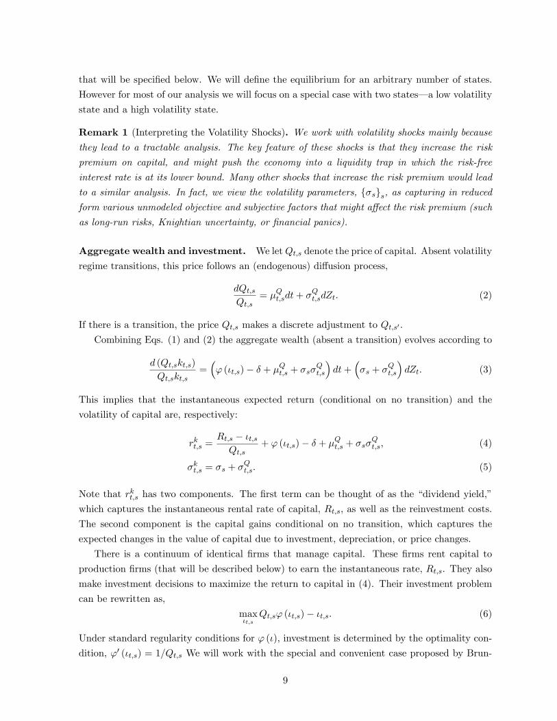
Figure 2: The left panel illustrates the effect of optimism on the asset price in state 2. Theright panel illustrates the effect of risk premium on the asset price in state 2, when optimism ishigher (solid line) and lower (dashed line).

of optimism unleashes these forces and makes the equilibrium prices and output very sensitive

to exogenous changes in asset prices due to beliefs (as well as other factors). The left panel of

Figure 2 illustrates these results for a particular parameterization.

Next consider the effect of an increase in the risk premium in the high-risk state. In our

model, the risk premium is equal to the variance, σ22 (Eq. (28)). Following the same steps as

above, we obtain,dq2

d(σ2

2

) =−1

−∂R (q2, q∗, λ2) /∂q2< 0. (32)

Greater risk premium reduces the price due to its direct effect on the risk-adjusted return. As

before, the effect is stronger when optimism is lower due to endogenous destabilizing forces.

Formally, we have, ddλ2

∣∣∣∣ dq2d(σ22)

∣∣∣∣ < 0. Combining Eqs. (31) and (32), we also obtain that the

effect is stronger when the baseline level of the risk premium is higher (as this leads to a lower

price level, q2).8 Formally, we have dd(σ22)

∣∣∣∣ dq2d(σ22)

∣∣∣∣ > 0. The right panel of Figure 2 illustrates

these results. Note that, for each level of optimism, there is a suffi ciently high level of the

risk premium that ensures Assumption 2 holds as equality and the economy experiences a deep

recession. Beyond this level of the risk premium, there is no equilibrium with positive prices.

8To understand the intuition, note from Eq. (27) that the expected capital gains are given byλ2 (1− exp (q2 − q∗)). When q2 is lower (due to higher σ22), the capital gain conditional on a transition is alreadyhigh and it is not very sensitive to further changes to q2. On the other hand, the strength of the destabilizingaggregate demand and growth forces is controlled by the parameter, ψ, which is independent of the level of q2.

19

Corollary 1. (i) A decrease in optimism in state 2 reduces the price level, that is, dq2dλ2

> 0.

(ii) An increase in the risk premium in state 2 reduces the price level, that is, dq2d(σ2)2

< 0;

and by a larger magnitude when optimism is lower and the risk premium is higher, that is,ddλ2

∣∣∣∣ dq2d(σ22)

∣∣∣∣ < 0 and dd(σ22)

∣∣∣∣ dq2d(σ22)

∣∣∣∣ > 0.

Note also that, as illustrated by Eq. (29), these changes that reduce the price in the high-

volatility state, q2, also reduce the interest rate in the low-volatility state, r1f . Intuitively, lower

prices in state 2 also lower the asset prices and aggregate demand in state 1, which is countered

by a lower interest rate.

4. Belief disagreements and speculation

We next consider the equilibrium with belief disagreements. As in the previous section, we first

provide a general characterization. We then explicitly solve for the equilibrium for the special

case with two states, S = {1, 2}.The equilibrium depends on the wealth-weighted average transition probability,

λt,s,s′ =∑i

αit,sλis,s′ , where α

it,s =

ait,skt,sQt,s

.

Here, αit,s denotes the wealth share of type i investors. Combining the optimality conditions

(13) and (14) with the market clearing conditions (20) and (21), we obtain,

ps′t,s = λis,s′

ait,sait,s′

= λt,s,s′Qt,sQt,s′

, (33)

σs + σQt,s =1

σs + σQt,s

(rkt,s − r

ft,s +

∑s′

λt,s,s′

(1− Qt,s

Qt,s′

)), (34)

ωk,it,s = 1 for each t, s, i.

The first equation says that the price of the Arrow-Debreu security is determined by the weighted

average belief for the transition probability. The second equation says that the risk balance

equation (25) in the benchmark case continues to hold in this setting as long as we calculate the

transition probability with the weighted average belief. The last equation says that investors

continue to allocate identical weights to capital. Intuitively, since their disagreements concern

the jump probabilities, they use the Arrow-Debreu securities to speculate on these disagreements

and do not distort their exposures to the diffusion risk.

It remains to characterize the evolution of the investors’wealth shares, αit,s. Plugging the

evolution of wealth equation (10) into Eq. (33), and using ωk,it,s = 1, we obtain,

ωs′,it,s = λis,s′ − λt,s,s′ . (35)

20

That is, the investor’s wealth share in the Arrow-Debreu security is equal to her degree of

optimism relative to the weighted average belief. Combining this with Eq. (10), we further

obtain, dαit,sαit,s

= −∑

s′ 6=s(λis,s′ − λt,s,s′

)dt, if there is no state change,

αit,s′ = αit,sλis,s′

λt,s,s′, if there is a state change to s′.

(36)

In particular, conditional on there not being a state change, the wealth shares evolve determin-

istically. If the investor is relatively optimistic about state transitions, then her wealth declines

conditional on these transitions not being realized. However, when a state on which the investor

is optimistic is eventually realized, the investor’s wealth share makes a discrete upward jump.

The symmetric opposite considerations apply to the wealth share of an investor that is relatively

pessimistic.

The equilibrium is then characterized as follows. Regardless of the level of asset prices and

output, Eq. (36) determines the evolution of investors’wealth shares. This in turn determines

the weighted average belief, λt,s,s′ , as well as its evolution. Given the path of the weighted-average

belief,{λt,s,s′

}t, the equilibrium is determined by jointly solving the risk balance equation (34)

and the goods market equilibrium condition (23). Solving these equations is slightly more

involved than in the previous section since the weighted-average belief is generally not stationary,

which implies the price of capital might also have a nonzero drift, µQt,s (although σQt,s is zero as

before).

Two-states special case. To characterize the equilibrium further, consider the special case

with two states S = {1, 2}, with σ1 < σ2 from the previous section. Recall that we also use

the shorthand notations, λ1 = λ1,2 and λ2 = λ2,1, to denote the transition rates respectively in

states 1 and 2 (into the other state). Suppose there are two types of investors, i ∈ {o, p}, withbeliefs denoted by,

{(λi1, λ

i2

)}i∈{o,p}. Here, type o investors correspond to “optimists,”and type

p investors correspond to “pessimists.”We denote optimists’transition probability relative to

pessimists with the notation,

∆λs = λos − λps,

and assume beliefs satisfy the following.

Assumption 4. ∆λ2 > 0 and ∆λ1 ≤ 0.

This assumption ensures that optimists are more optimistic than pessimists in either state.

Specifically, when the economy is in the high-volatility state, optimists find the transition into

the low-volatility state relatively likely (λo2 > λp2); when the economy is in the low-volatility

state, optimists find the transition into the high-volatility state relatively unlikely (λo1 ≤ λp1).

For notational simplicity, we use αt,s = αot,s ∈ (0, 1) to represent optimists’wealth share.

21

Note that the weighted-average belief can be written as,

λt,s = λps + αt,s∆λs. (37)

Hence, optimists’wealth share denotes the appropriate state variable in this economy. By Eq.

(35), optimists’investment in the contingent security is given by,

ωs′,ot,s = ∆λs (1− αt,s) ,

and by Eq. (36), their wealth share evolves according to,{αt,s = −∆λsαt,s (1− αt,s) , if there is no state change,

αt,s′ = αt,sλos/ (λps + αt,s∆λs) , if there is a state change to s′.

(38)

Here, αt,s =dαt,sdt denotes the derivative with respect to time. Recall that ∆λ1 ≤ 0 and ∆λ2 > 0

(see Assumption 4). Hence, in the low-volatility state 1, optimists’wealth share drifts upwards,

but it makes a downward jump if there is a transition into state 2. Intuitively, optimists sell

put options on the aggregate state, which enables them to earn current profits at the expense

of losses if the bad aggregate state is realized. Symmetrically, in the high-volatility state 2,

optimists’wealth share drifts downwards but it makes an upward jump in case there is transition

into state 1. Intuitively, optimists buy call options on the aggregate state, which reduces their

current profits but generates gains if the good aggregate state is realized.

These observations also imply that the weighted-average belief in (37) (that determines asset

prices) is effectively extrapolative. As the good (low-volatility) state persists longer, and opti-

mists’wealth share increases, the aggregate belief becomes increasingly more optimistic. After

a transition to a worse (high-volatility) state, the aggregate belief becomes more pessimistic.

Conversely, the aggregate belief becomes more pessimistic as the bad state persists longer, and

it becomes more optimistic after a transition into a better (low-volatility) state.

We next characterize the equilibrium (log) prices and factor utilizations within each state,{qt,s, ηt,s

}s∈{1,2}. To this end, suppose Assumptions 1-3 hold according to optimists’as well as

pessimists’beliefs. This ensures that, regardless of the wealth shares, state 1 features a positive

interest rate, effi cient price level, and full factor utilization, rft,1 > 0, qt,1 = q∗, and ηt,1 = 1. We

also conjecture that state 2 features a zero interest rate, a lower price level, and imperfect factor

utilization, rft,2 = 0, qt,2 < q∗, and ηt,1 < 1.

To characterize the price level in state 2, consider the risk balance equation (34). After

substituting the return to capital from (24), and using µQt,2 =dQt,2/dtQt,2

=dqt,2dt , we obtain,

rft,2 = R(qt,2, q

∗, λt,2)

+ qt,2 − σ22 = 0. (39)

Here, R (·) is the function that characterizes the expected return to capital in the homogeneous

22

0 0.2 0.4 0.6 0.8 1

0.85

0.9

0.95

1

1.05

1.1

1.15

1.2

1.25

1.3

1.35

0 0.2 0.4 0.6 0.8 1­0.01

0

0.01

0.02

0.03

0.04

0.05

0.06

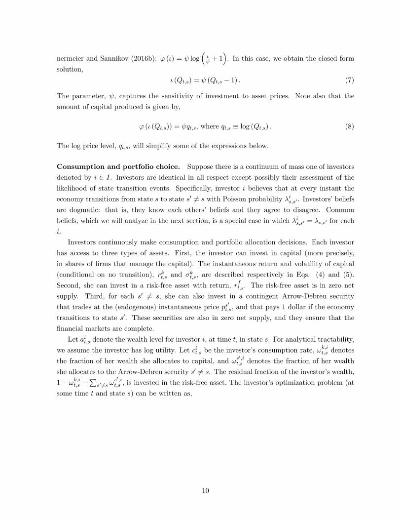
Figure 3: The solid lines illustrate the equilibrium price and interest rate functions under het-erogeneous beliefs. The dashed line in the left panel illustrates the equilibrium price level thatwould obtain if all investors shared the weighted-average belief, λt,2.

beliefs benchmark (cf. (27)), and qt,2 =dqt,2dt denotes the price drift conditional on there not

being a transition. Eq. (39) illustrates that the expected return to capital is related to but not

exactly the same as the return that would obtain in the benchmark in which all investors shared

the weighted-average belief, λt,2. In the present setting, the expected return (and thus, the

equilibrium condition) is also affected by the wealth dynamics that change the weighted-average

belief and ultimately introduce a drift into the asset price.

In particular, consider the joint evolution of optimists’wealth share and the price level con-

ditional on there not being a state transition, denoted by (αt,2, qt,2). Combining Eqs. (38− 39),

we obtain a stationary differential equation,

qt,2 = −(R (qt,2, q

∗, λp2 + αt,2∆λ2)− σ22

), (40)

αt,2 = −∆λ2αt,2 (1− αt,2) .

In Appendix B, we show that this system is saddle path stable. In particular, for any initial

wealth share, αt,2 ∈ (0, 1), there exists a unique equilibrium price level, qt,2 ∈ [qp, qo), such that

the solution satisfies limt→∞ αt,2 = 0 and limt→∞ qt,2 = qp2 . When αt,2 = 1, the solution satisfies

qt,2 = qot .

Since the system in (40) is stationary, the equilibrium price can be written as a function of

optimists’wealth share, that is, qt,2 = q2 (αt,2) for some function q2 : [0, 1]→ [qp, qo]. Eliminating

23

time from the system , the price function solves the differential equation,

q′2 (α) ∆λ2α (1− α) = R (q2 (α) , q∗, λp2 + α∆λ2)− σ22, (41)

together with the end-value conditions, q2 (0) = qp2 and q2 (1) = qo2. In Appendix B, we show that

the price function, q2 (α), is strictly increasing in α. As in the previous section, greater optimism

increases the asset price in state 2. We also show that q2 (α) < qh2 (α) for each α ∈ (0, 1),

where qh2 (α) denotes the price level that would obtain in the homogeneous belief benchmark

in which all investors share the belief, λp2 + α∆λ2. Intuitively, if the recession persists longer,

pessimists will become more dominant and the price level will drift downward. The downward

drift reduces the return to capital, which reduces the current price level to equilibrate the risk

balance condition. This illustrates that, when output is demand constrained, speculation driven

by belief disagreements reduces aggregate demand and output as well as asset prices.

The left panel of Figure 3 illustrates the price function, q2 (α), for a particular parameteri-

zation. We chose the parameters so that pessimists’belief in state 2, λp2, satisfies Assumption

2 with equality. This implies that, when optimists’wealth share is low, asset prices and output

are very low due to the destabilizing forces that we discussed in the previous section. The fig-

ure further illustrates that the equilibrium with heterogeneous beliefs differs sharply from the

homogeneous beliefs benchmark in which all investors share the weighted average belief. In the

benchmark, optimism greatly improves the outcomes by mitigating the destabilizing forces (see

Section 3). With heterogeneous beliefs, optimism has a smaller effect since the investors recog-

nize that, if the recession persists, pessimism will prevail and unleash the destabilizing forces.

This suggests that it is enough to have one group of highly pessimistic agents to unleash the

destabilizing aggregate demand and growth forces.

For completeness, we also characterize the equilibrium interest rate in state 1. Following

similar steps, we obtain, rft,1 = rf1 (αt,1) where rf1 : [0, 1]→ R+ denotes the function defined by,

rf1 (α) = R(q∗, q2

(α′), λp1 + α∆λ1

)− σ2

1 where α′ = αλo1/ (λp1 + α∆λ1) . (42)

Here, q2 (α′) captures the price that would obtain if there was an immediate transition into

state 2. Since there is no price drift in state 1, the return to capital is characterized as in the

homogeneous beliefs benchmark given the weighted average belief and the endogenous transition

price. The risk-free interest rate is equal to the return to capital net of the risk premium. For

our conjecture to be valid, we also require, rf1 (α) > 0 for each α. This condition holds because

Assumptions 1-3 hold for pessimists (as well as optimists). The right panel of Figure 3 illustrates

the interest-rate function. The following result summarizes the characterization of equilibrium.

Proposition 2. Consider the model with two states, s ∈ {1, 2}, and heterogeneous beliefs.Suppose Assumptions 1-3 hold for each belief type i ∈ {i, o}, and that beliefs are ranked ac-cording to Assumption 4. Then, optimists’ wealth share evolves according to Eq. (38). The

24

0 10 20 30 40 501

1.5

2

0 10 20 30 40 500

0.5

1

0 10 20 30 40 500.9

11.11.21.3

0 10 20 30 40 50

Year t

­0 .010

0.010.020.03

0.5 1 1.5 2 2.50

0.5

1

0 0.2 0.4 0.6 0.8 10

2

4

0 0.2 0.4 0.6 0.8 10

2

4

­0 .01 0 0.01 0.02 0.030

50

Figure 4: The left panels illustrate the evolution of the equilibrium variables over the mediumrun (50 years) for a particular realization of uncertainty. The right panels illustrate the long-runstationary distributions of equilibrium variables.

equilibrium prices and interest rates can be written as a function of optimists’ wealth shares,

q1 (α) , rf1 (α) , q2 (α) , rf2 (α). At the high-volatility state, rf2 (α) = 0 and q2 (α) solves the differ-

ential equation (39) with q2 (0) = qp2 and q2 (1) = qo2. The price function satisfiesdq2(α)dα > 0

and q2 (α) < qh2 (α) for each α ∈ (0, 1) (where qh2 (α) denotes the price in the homogeneous-

belief benchmark with wealth-weighted average belief, λp2 + α∆λ2). At the low-volatility state,

q1 (α) = q∗ and rf1 (α) is given by Eq. (42). The interest rate function satisfies drf1 (α)dα > 0 for

each α ∈ (0, 1).

Dynamics of equilibrium. Figure 4 illustrates the dynamics of the equilibrium. The panels

on the left illustrates the evolution of the equilibrium variables over a 50-year horizon. Note

that optimists’wealth share grows in the low-volatility state but it declines when the economy

switches to the high-volatility state. The asset price is below its effi cient level in the high-

volatility state, and more so when optimists’wealth share is lower. The panels on the right

illustrate the simulated long-run distributions of equilibrium variables. To obtain non-degenerate

long-run wealth distribution, in which neither optimists nor pessimists permanently dominate,

we simulate the economy with beliefs that are in the “middle” of optimists’ and pessimists’

beliefs in terms of the relative entropy distance.9 Note that the economy spends relatively little

time in the range in which optimists’wealth share is in the intermediate range. Intuitively, this9Given two probability distributions (p (s))s∈S and (q (s))s∈S , relative entropy of p with respect to q is defined as∑s p (s) log

(p(s)q(s)

). Blume and Easley (2006) show that, in a setting with independent and identically distributed

shocks (and identical discount factors), only investors whose beliefs have the maximal relative entropy distanceto the true distribution survive. Since our setting features Markov shocks, we apply their result state-by-state to

25

0 0.2 0.4 0.6 0.8 1  ­1

­0.5

   0

 0.5

   1

0 0.2 0.4 0.6 0.8 1 ­0.003

­0.0025

 ­0.002

­0.0015

 ­0.001

­0.0005

      0

0 0.2 0.4 0.6 0.8 1­0.008

­0.006

­0.004

­0.002

     0

 0.002

0 0.2 0.4 0.6 0.8 1­0.00025

 ­0.0002

­0.00015

 ­0.0001

  ­5e­05

       0

   5e­05

Figure 5: The effect of making optimists less optimistic in state 1 (top panels) and in state 2(bottom panels).

range features substantial speculation, which is resolved only when one or the other belief type

temporarily dominates. Note also that optimists tend to dominate more in the low-volatility

state 1, whereas pessimists tend to dominate more in the high-volatility state 2. In the next

section, we will investigate whether and how macroprudential policy can affect the evolution of

investors’wealth shares.

Comparative statics of equilibrium. To facilitate our analysis of macroprudential policy,

we also establish the comparative statics of reducing optimists’ optimism. First consider a

decline in their optimism in state 1 (captured by an increase in the transition probability, λo1). As

illustrated by the top panels of Figure 5, this leaves the price function in state 2 unchanged (since

the beliefs in that state are unchanged) but it reduces the risk-free rate in state 1. Intuitively,

lower optimism reduces the demand for risky assets in state 1 but this effect is countered by a

reduction in the interest rate. Next consider a decline in optimists’optimism in state 2 (captured

by a decrease in the transition probability, λo2). As illustrated by the bottom panels of Figure 5,

this reduces the price function in state 2 as well as the interest rate function in state 1. These

results are similar to the effect of reducing optimism in state 2 in the common beliefs benchmark

(cf. Corollary 1). Note also that, as expected, reducing an investor’s optimism has a greater

impact on prices when their wealth share is higher.

ensure that conditional probabilities satisfy the necessary survival condition. Specifically, for each state s ∈ {1, 2},we choose λsims so that the relative entropy of the conditional probability distribution for the next state withrespect to optimists’beliefs (in the discrete-time approximation of the model) is the same as the relative entropywith respect to pessimists’beliefs.

26

5. Welfare analysis and macroprudential policy

In this section, we establish our normative results on macroprudential policy. To this end, we

first characterize investors’ value functions in equilibrium. This establishes the determinants

of welfare in this setting and illustrates the aggregate demand externalities. We then show

that, when investors have heterogeneous beliefs, the equilibrium can be Pareto improved by

macroprudential policy that restricts optimists’risk taking. Throughout, we focus on the two-

state special case to simplify the notation.

5.1. Equilibrium value functions

Recall that the value function has the functional form in (11), where vit,s denotes the normalized

value function per unit of capital stock. Eq. (A.12) in Appendix A.2 characterizes vit,s as a

solution to a differential equation. In the two-state special case, the equation becomes,

ρvit,s −∂vit,s∂t

= log ρ+ qt,s +1

ρ

ψqt,s − δ − 12σ

2s

−(λis − λt,s

)+ λis log

(λisλt,s

) + λis(vit,s′ − vit,s

). (43)

The equilibrium value functions for type i are characterized by jointly solving the differential

equations for states s ∈ {1, 2}.Eq. (43) illustrates the determinants of welfare. When there is a demand-driven recession

(qt,s ≤ q∗), a lower equilibrium price, qt,s, reduces investors’welfare since it is associated with

lower factor utilization, ηt,s. Note that welfare declines due to a decline in current consump-

tion (captured by the term, log ρ + qt,s) as well as a decline in investment and consumption

growth (captured by the term, ψqt,s − δ = gt,s). The risk premium, σ2s, also affects the wel-

fare through its influence on the risk-adjusted consumption growth. Finally, speculation among

investors with heterogeneous beliefs also affects (perceived) welfare. This is captured by the

term, −(λis − λt,s

)+λis log

(λisλt,s

), which is zero with common beliefs, and strictly positive with

heterogeneous beliefs.

To facilitate our analysis of macroprudential policy, we also break down the value function

into two components,

vt,s = v∗t,s + wt,s, (44)

where v∗t,s denotes the first-best value function that would obtain if there were no interest rate

rigidities, and wt,s = vt,s − v∗t,s denotes the gap value function relative to the first best. Recallthat the first-best equilibrium features qt,s = q∗ for each t and s. Hence, the value function,

v∗t,s, is characterized as the solution to Eq. (43) with the effi cient price level, qt,s = q∗. Using

linearity, the gap value function is then characterized as the solution to the following differential

equation,

ρwit,s −∂wit,s∂t

=

(1 +

ψ

ρ

)(qt,s − q∗) + λis

(wit,s′ − wit,s

). (45)

27

This illustrates that the gap value captures the loss of welfare due to the price deviations from

the first best. The first best value, vi,∗t,s , captures the remaining components of value including

the perceived welfare from speculation. As we will see, the gap value functions are useful to

understand the marginal effect of macroprudential policy on social welfare.

We next characterize the value function and its components in the equilibria we analyzed in

the previous sections.

Value functions in the common beliefs benchmark. With common beliefs, the price

level is stationary, qt,s = qs for each s (see Section 3). Eq. (43) then implies that the value

function is also stationary, vt,s = vs for each s. In Appendix A.2, we show that the stationary

values can be solved in closed form as,

ρvs = log ρ+ qs +1

ρ

(ψqs − δ −

1

2σ2s

), (46)

where qs = βsqs + (1− βs) qs′ and σ2s = βsσ

2s + (1− βs)σ2

s′ ,

and βs =ρ+ λs′

ρ+ λs′ + λs.

Here, the weights βs and 1 − βs can be thought of as capturing the expected amount of “dis-counted time” the investor spends in each state (the weights reflect the fact that the investor

starts in state s and discounts the future at rate ρ). The value in a state is the sum of the utility

from (the discounted average of) current consumption and the present value of the risk-adjusted

growth rate. All else equal, the value is decreasing in the weighted average volatility, σs, but it

is increasing in the weighted-average price level, qs.

It can also be seen that the first-best and the gap value components are stationary, v∗t,s = v∗sand w∗t,s = w∗s . Using Eq. (45), we further obtain,

ρws = (qs − q∗)(

1 +ψ

ρ

). (47)

That is, the gap value is proportional to the weighted-average price gap relative to the first best.

In Appendix A.2, we further show that w2 < w1 < 0, that is, the gap value is negative for both

states but more negative in the high-volatility state.

Value functions with two belief types and aggregate demand externalities. With

heterogeneous beliefs, the solution to Eq. (43) is not necessarily stationary since the price might

have a drift. Consider the equilibrium with two belief types that we analyzed in Section 4.

Recall that the equilibrium price in the high-volatility state is a function of optimists’wealth

share, q2 (α). The equilibrium values and its components can also be written as a function of

optimists’wealth share,{vis (α) , vi,∗s (α) , ws (α)

}s,i. Appendix A.2 characterizes these value

functions as solutions to differential equations in α-domain (by combining Eqs. (43) and (45)

28

0 0.2 0.4 0.6 0.8 1

­40

­30

­20

­10

Value for s=1

0 0.2 0.4 0.6 0.8 1­14

­12

­10

­8

­6

­4

­2

0

0 0.2 0.4 0.6 0.8 1

­40

­30

­20

­10

Value for s=2

0 0.2 0.4 0.6 0.8 1­20

­15

­10

­5

0

Figure 6: The plots illustrate the equilibrium value functions for each state and belief type.The solid lines are the actual value functions, vis (α), the dotted lines are the first-best valuefunctions, vi,∗s (α), and the dashed lines (in the bottom panels) are the gap value functions,wis (α).

with the evolution of αt,s from (38)). Figure 6 illustrates the solution to these differential

equations for the equilibrium plotted in the earlier Figure 3.

The bottom panels of Figure 6 show that the gap value functions are increasing in the wealth

share of optimists, α, which illustrates the aggregate demand externalities. Greater α increases

the effective optimism, which in turn leads to a greater equilibrium asset price in the high-

volatility state (see Figure 3). This improves the gap value function in this state by raising the

aggregate demand and bringing the economy closer to the first-best benchmark (see Eq. (45)).

It also improves the gap value function in the low-volatility state, because the economy can

always transition into the high-volatility state, and these transitions are less costly when α is

greater. Hence, increasing optimists’wealth share is always associated with positive aggregate

demand externalities. Individual optimists that take risks (or pessimists that take the other side

of these trades) do not internalize their effects on asset prices, which leads to ineffi ciencies and

generates scope for macroprudential policy.

The top panels of Figure 6 illustrate that the first-best value functions are increasing in α for

pessimists but it is decreasing in α for optimists. These effects can be understood via pecuniary

externalities in contingent security markets. Increasing the mass of optimists increases the

price of contingent securities that optimists purchase, while decreasing the price of contingent

securities that pessimists purchase. This creates negative pecuniary externalities (or crowd-out

effects) on optimists, and positive pecuniary externalities on pessimists.

Finally, note that the actual value function is the sum of the first-best and the gap value

29

functions. For pessimists, the actual value is always increasing in α, since the two components

move in the same direction. For optimists, this is not necessarily the case since the gap value is

increasing in α whereas the first-best value is decreasing.

5.2. Macroprudential policy

We capture macroprudential policy as risk limits on optimists. Consider the case with two

belief types. Suppose, at any state s and time t, the planner can induce optimists to choose

(instantaneous) allocations as if they have less optimistic beliefs. Specifically, optimists are

constrained to choose allocations as if they have beliefs,(λo,plt,1 , λ

o,plt,2

), that satisfy, λo,plt,1 ≥ λo1

and λo,plt,2 ≤ λo2. In Appendix A.3, we show that the planner can implement this policy by

imposing inequality restrictions on optimists’portfolio weights (see Eq. (A.18)), while allowing

them to make unconstrained consumption-savings decisions. Specifically, the policy constrains

optimists from taking too low a position on the contingent security that pays in the high-volatility

state, ω2,ot,1 ≥ ω

2,ot,1 (restrictions on selling “put options”). It also constrains optimists from taking

too high a position on the contingent security that pays in the low-volatility state, ω1,ot,2 ≤ ω1,o

t,2

(restrictions on buying “call options”). Finally, the policy also constrains optimists’position on

capital not to exceed the market average, ωk,ot ≤ 1 (since otherwise optimists start to speculate

by holding too much capital).

For simplicity, we restrict attention to time-invariant policies. Specifically, the planner com-

mits to a policy at time zero, λo,pl ≡(λo,pl1 , λo,pl2

), and implements it throughout. We assume the

planner respects investors individual beliefs, that is, optimists’as well as pessimists’expected

values in equilibrium are calculated according to their own beliefs. Finally, to trace the Pareto

frontier, we also allow the planner to do a one-time wealth transfer among the agents at time

zero.

Formally, let V it,s

(ait,s|λo,pl

)denote type i investors’expected value in equilibrium when she

starts with wealth ait,s and the policy is λo,pl. The planner’s Pareto problem can then be written

as,

maxλo,pl

,α0,s

γoV o0,s

(α0,sQ0,sk0,s|λ

o,pl)

+ γpV p0,s

((1− α0,s)Q0,sk0,s|λ

o,pl). (48)

Here, γo, γp ≥ 0 (with at least one strict inequality) denote the Pareto weights, and Q0,s denotes

the endogenous equilibrium price that obtains under the planner’s policy.

The characterization of equilibrium with policy is the same as in Section 4. In particular,

Eqs. (38) and (39) continue to hold with the only difference that optimists’beliefs are replaced

by their “as-if”beliefs,(λo,pl1 , λo,pl2

). The main difference in this case concerns the calculation

of value functions, which are determined according to investors’actual beliefs. We start with a

number of observations that simplify the welfare analysis.

First, the value function has the same functional form as before with appropriate normalized

value functions, vit,s. After substituting ait,s = αit,skt,sQt,s, the functional form in (11) can be

30

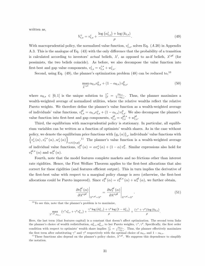
written as,

V it,s = vit,s +

log(αit,s)

+ log (kt,s)

ρ. (49)

With macroprudential policy, the normalized value function, vit,s, solves Eq. (A.20) in Appendix

A.3. This is the analogue of Eq. (43) with the only difference that the probability of a transition

is calculated according to investors’ actual beliefs, λi, as opposed to as-if beliefs, λi,pl (for

pessimists, the two beliefs coincide). As before, we also decompose the value function into

first-best and gap value components, vit,s = vi,∗t,s + wit,s.

Second, using Eq. (49), the planner’s optimization problem (48) can be reduced to,10

maxλo,pl

α0,svo0,s + (1− α0,s) v

p0,s, (50)

where α0,s ∈ [0, 1] is the unique solution to γo

γp =α0,s

1−α0,s . Thus, the planner maximizes a

wealth-weighted average of normalized utilities, where the relative wealths reflect the relative

Pareto weights. We therefore define the planner’s value function as a wealth-weighted average

of individuals’value functions, vplt,s = αt,svot,s + (1− αt,s) vpt,s. We also decompose the planner’s

value function into first-best and gap components, vplt,s = vpl,∗t,s + wplt,s.

Third, the equilibrium with macroprudential policy is stationary. In particular, all equilib-

rium variables can be written as a function of optimists’wealth shares. As in the case without

policy, we denote the equilibrium price functions with {qs (α)}s, individuals’value functions with{vis (α) , vi,∗s (α) , wis (α)

}s,i∈{o,p}

.11 The planner’s value function is a wealth-weighted average

of individual value functions, vpls (α) = αvos (α) + (1− α) vps . Similar expressions also hold for

vpl,∗s (α) and wpls (α).

Fourth, note that the model features complete markets and no frictions other than interest

rate rigidities. Hence, the First Welfare Theorem applies to the first-best allocations that also

correct for these rigidities (and features effi cient output). This in turn implies the derivative of

the first-best value with respect to a marginal policy change is zero (otherwise, the first-best

allocations could be Pareto improved). Since vpls (α) = vpl,∗s (α) + wpls (α), we further obtain,

∂vpls (α)

∂λo,pl

∣∣∣∣∣λo,pl=λo

=∂wpls (α)

∂λo,pl

∣∣∣∣∣λo,pl=λo

. (51)

10To see this, note that the planner’s problem is to maximize,

maxλo,pl

,α0,s

(γovo0,s + γpvp0,s

)+γo log

(αo0,s

)+ γp log

(1− αo0,s

)ρ

+(γo + γp) log (k0,s)

ρ.

Here, the last term (that features capital) is a constant that doesn’t affect optimization. The second term linksthe planner’s choice of wealth redistribution, αo0,s, α

p0,s, to her Pareto weights, γ

o, γp. Specifically, the first order

condition with respect to optimists’wealth share implies γo

γp=

α0,s1−α0,s . Thus, the planner effectively maximizes

the first term after substituting γo and γp respectively with the optimal choice of α0,s and 1− α0,s.11These functions also depend on the planner’s policy choice, λo,pl. We suppress this dependence to simplify

the notation.

31

The upshot of these observations is that the marginal effect of policy is determined by its

marginal effect on the planner’s gap value function, which can be written as,

wpls (α) = αwos (α) + (1− α)wps (α) .

In Appendix A.3, we show that the gap value function is characterized as the solution to the

same HJB equation (45) as before (determined by investors’ actual beliefs, λis). Intuitively,

macroprudential policy affects the path of prices, qt,s, but it does not change the characterization

of the gap values conditional on these prices. Combining Eq. (45) with the evolution of optimists’

wealth share in (38) (which is determined by the as-if beliefs, λi,pls ), we obtain the differential

equation system,

ρwis (α) =

(1 +

ψ

ρ

)(qs (α)− q∗)− α (1− α) ∆λpls

∂wis (α)

∂α+ λis

(wis′(α′)− wis (α)

). (52)

Here, α′ = α λo,pls

λps+α∆λplsdenotes optimists’wealth share after a transition evaluated under the

as-if beliefs. It remains to characterize how macroprudential policy affects the solution to the

system in (52). We start by analyzing the effect of macroprudential policy in the low-volatility

state s = 1, assuming that there is no intervention in the other state. We then analyze the polar

opposite case in which there is intervention in the high-volatility state s = 2 but not the other

state.

5.2.1. Macroprudential policy during the boom

Suppose the planner is constrained to set λo,pl2 = λo2, but she can choose λo,pl1 ≥ λo1, which induces

optimists to act more pessimistically in the low-volatility state. First consider the special case,

∆λ1 = 0 (so investors disagree only in state s = 2). We obtain a sharp result for this case, and

we show in numerical simulations that the result also applies when ∆λ1 < 0.

Proposition 3. Consider the equilibrium with heterogeneous beliefs that satisfy ∆λ1 = 0 (so

disagreements only concern transitions out of state s = 2), together with macroprudential policy

that satisfies λo,pl2 = λo2 (so policy affects only λo,pl1 ). Macroprudential policy strictly increases

the gap value according to each belief, that is,

∂wis (α)

∂λo,pl1

∣∣∣∣∣λo,pl=λo

> 0 for each i ∈ {o, p} , s ∈ {1, 2} and α ∈ (0, 1) .

Macroprudential policy also increases the planner’s value, ∂vpls (α)

∂λo,pl

∣∣∣λo,pl=λo

= ∂wpls (α)

∂λo,pl

∣∣∣λo,pl=λo

> 0.

In particular, regardless of the planner’s Pareto weight and the current state, there exists a

Pareto improving macroprudential policy, λo,pl1 .

The result shows that macroprudential policy improves the gap value function according

32

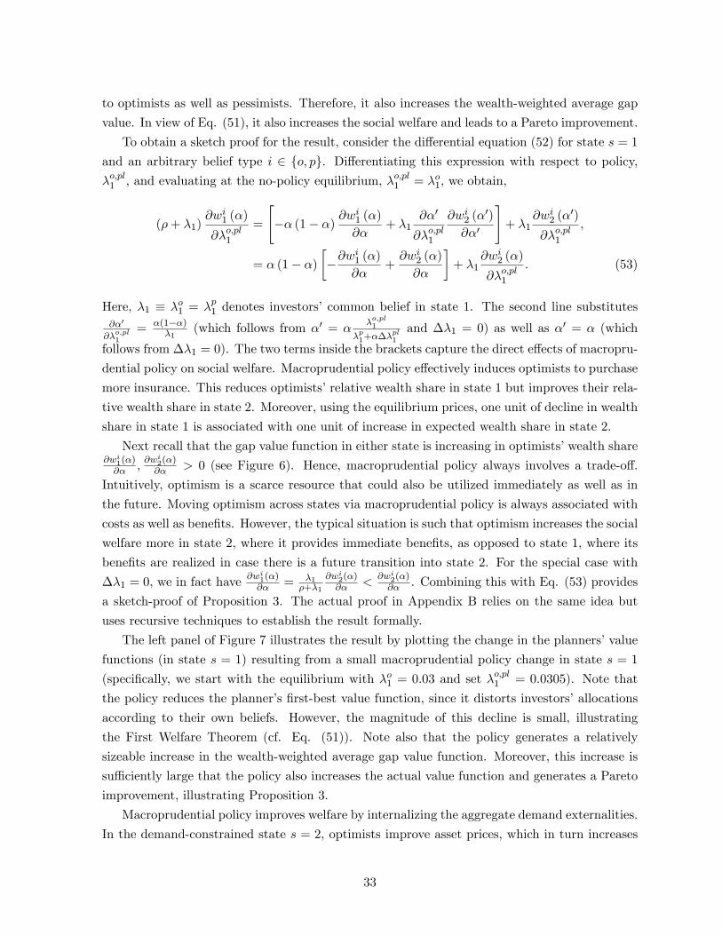
to optimists as well as pessimists. Therefore, it also increases the wealth-weighted average gap

value. In view of Eq. (51), it also increases the social welfare and leads to a Pareto improvement.

To obtain a sketch proof for the result, consider the differential equation (52) for state s = 1

and an arbitrary belief type i ∈ {o, p}. Differentiating this expression with respect to policy,λo,pl1 , and evaluating at the no-policy equilibrium, λo,pl1 = λo1, we obtain,

(ρ+ λ1)∂wi1 (α)

∂λo,pl1

=

[−α (1− α)

∂wi1 (α)

∂α+ λ1

∂α′

∂λo,pl1

∂wi2 (α′)

∂α′

]+ λ1

∂wi2 (α′)

∂λo,pl1

,

= α (1− α)

[−∂w

i1 (α)

∂α+∂wi2 (α)

∂α

]+ λ1

∂wi2 (α)

∂λo,pl1

. (53)

Here, λ1 ≡ λo1 = λp1 denotes investors’common belief in state 1. The second line substitutes∂α′

∂λo,pl1

= α(1−α)λ1

(which follows from α′ = αλo,pl1

λp1+α∆λpl1and ∆λ1 = 0) as well as α′ = α (which

follows from ∆λ1 = 0). The two terms inside the brackets capture the direct effects of macropru-

dential policy on social welfare. Macroprudential policy effectively induces optimists to purchase

more insurance. This reduces optimists’relative wealth share in state 1 but improves their rela-

tive wealth share in state 2. Moreover, using the equilibrium prices, one unit of decline in wealth

share in state 1 is associated with one unit of increase in expected wealth share in state 2.

Next recall that the gap value function in either state is increasing in optimists’wealth share∂wi1(α)∂α ,

∂wi2(α)∂α > 0 (see Figure 6). Hence, macroprudential policy always involves a trade-off.

Intuitively, optimism is a scarce resource that could also be utilized immediately as well as in

the future. Moving optimism across states via macroprudential policy is always associated with

costs as well as benefits. However, the typical situation is such that optimism increases the social

welfare more in state 2, where it provides immediate benefits, as opposed to state 1, where its

benefits are realized in case there is a future transition into state 2. For the special case with

∆λ1 = 0, we in fact have ∂wi1(α)∂α = λ1

ρ+λ1

∂wi2(α)∂α <

∂wi2(α)∂α . Combining this with Eq. (53) provides

a sketch-proof of Proposition 3. The actual proof in Appendix B relies on the same idea but

uses recursive techniques to establish the result formally.

The left panel of Figure 7 illustrates the result by plotting the change in the planners’value

functions (in state s = 1) resulting from a small macroprudential policy change in state s = 1

(specifically, we start with the equilibrium with λo1 = 0.03 and set λo,pl1 = 0.0305). Note that

the policy reduces the planner’s first-best value function, since it distorts investors’allocations

according to their own beliefs. However, the magnitude of this decline is small, illustrating

the First Welfare Theorem (cf. Eq. (51)). Note also that the policy generates a relatively

sizeable increase in the wealth-weighted average gap value function. Moreover, this increase is

suffi ciently large that the policy also increases the actual value function and generates a Pareto

improvement, illustrating Proposition 3.

Macroprudential policy improves welfare by internalizing the aggregate demand externalities.

In the demand-constrained state s = 2, optimists improve asset prices, which in turn increases

33

0 0.2 0.4 0.6 0.8 1

­0.002

     0

 0.002

 0.004

 0.006

 0.008

  0.01

 0.012

 0.014

0.03 0.035 0.04 0.045 0.05

­0.5

­0.4

­0.3

­0.2

­0.1

0

0.1

0.2

0.3

0.4

Figure 7: The left panel illustrates the effect of a small change in macroprudential policy in state1 (λo,pl1 = 0.0305 where λo1 = 0.03) on the planner’s value functions. The right panel illustratesthe effect of larger changes as a function of policy.

aggregate demand and brings output closer to the first-best level. Individual optimists do not

internalize that they would improve asset prices and output by bringing more wealth into state

2. Macroprudential policy works by increasing optimists’insurance purchases, which increases

their wealth share in state 2. The result is reminiscent of the analysis in Korinek and Simsek

(2016), in which macroprudential policy improves outcomes by inducing agents that have a

high marginal propensity to consume (MPC) to bring more wealth into states in which there

is a demand-driven recession. However, the mechanism here is different and operates via asset

prices. In fact, in our setting, all investors have the same MPC equal to ρ. Optimists improve

aggregate demand not because they spend more than pessimists, but because they increase asset

prices and induce all investors to spend more, while also increasing aggregate investment and

hence growth.

As this discussion suggests, the parametric restriction, ∆λ1 = 0, is useful to obtain an an-

alytical result but it does not play a central role. We suspect that Proposition 3 also holds

absent this assumption, even though we are unable to provide a proof. In our numerical simula-

tions, we have not yet encountered a counterexample. The results displayed in Figure 7 actually

correspond to a parameterization with ∆λ1 < 0 (specifically, we have λo1 = 0.03 < λp1 = 0.075).

Proposition 3 concerns a small policy change. The right panel of Figure 7 illustrates the

effect of larger policies by plotting the changes in the planner’s value as a function of the size

of the policy (starting from, λo,pl1 = λo1). For this exercise, we fix the optimists’wealth share at

a particular level, α = 1/2. Note that, as the policy becomes larger, the gap value continues

to increase whereas the first-best value decreases. Moreover, the decline in the first-best value

34

0.03 0.04 0.05 0.06 0.07 0.08 0.09 0.10

1

2

3

4

5

6

7

0.03 0.04 0.05 0.06 0.07 0.08 0.09 0.10

1

2

3

4

5

6

0.03 0.04 0.05 0.06 0.07 0.08 0.09 0.10

0.2

0.4

0.6

0.8

1

1.2

Figure 8: The left panel illustrates the effect of macroprudential policy on social welfare whenall investors’value is calculated according to respectively optimists’or pessimists’belief. Thepanels on the right illustrate the effects on respectively the first-best and the gap value functions.

is negligible for small policy changes but it becomes sizeable for large policy changes. The

(constrained) optimal macroprudential policy obtains at an intermediate level, λo,pl,∗1 > λo1.

The figure also illustrates that the constrained optimal policy intervention is not too large

(specifically, we have λo,pl,∗1 = 0.0375 where λo1 = 0.03). This is typically the case in our numerical

simulations. The reason is that speculation generates high perceived utility for investors. Since

macroprudential policy restricts speculation, the perceived costs quickly rise with the degree of

the policy intervention, which implies that the optimal intervention is not too large.

Macroprudential policy according to a belief-neutral criterion. However, whether the

utility from speculation should be counted towards social welfare is questionable. A recent liter-

ature argues that the Pareto criterion is not the appropriate notion of welfare for environments

with belief disagreements. If investors’beliefs are different due to mistakes (say, in Bayesian

updating), then it is arguably more appropriate to evaluate investors’utility according to the

objective belief– which is common across the agents. Doing so would remove the speculative

utility from welfare calculations, and it could lead to a constrained optimal policy that is much

larger in magnitude. While reasonable, this approach faces a major challenge in implementation:

whose belief should the policymaker use?

In recent work, Brunnermeier et al. (2014) offer a belief-neutral welfare criterion that circum-

vents this problem. The basic idea is to require the planner to evaluate social welfare according

to a single belief, but also to make the welfare comparisons robust to the choice of the single

belief. Specifically, their baseline criterion says that an allocation is belief-neutral superior to

35

another allocation if it increases social welfare under every belief in the convex hull of investors’

beliefs. Proposition 3 suggests their criterion can also be useful in this context since macropru-

dential policy increases the gap value according to each belief– that is, the gap-reducing welfare

gains are belief neutral.

For a formal analysis, fix some h ∈ [0, 1] and let vis(α;λo,pl1 , λh

)denote the value function for

an individual when the planner implements policy, λo,pl1 , and evaluates utility under the belief

λh = λp + h (λo − λp) (calculated by replacing λis in Eq. (A.20) with λhs ). As before, define the

planner’s value function, vpls(α;λo,pl1 , λh

), as the wealth-weighted average of individual’s value

functions. Then, given the wealth share α (that corresponds to a particular Pareto weight), the

policy, λo,pl1 , is a belief-neutral improvement over some other policy, λo,pl1 , as long as,

vpl1

(α;λo,pl1 , λh

)> vpl1

(α; λ

o,pl1 , λh

)for each h ∈ [0, 1] . (54)

Figure 8 illustrates the belief-neutral optimal policy in the earlier example. The left panel

plots the effect of the policy on the social welfare (given α = 1/2) when the planner evaluates

all investor’s values under respectively pessimists’ belief (h = 0) and optimists’ belief (h =

1). The social welfare evaluated under intermediate beliefs lie in between these two curves.

As the figure suggests, tightening the policy towards λo,pl,neutral1 = 0.085 constitutes a belief-

neutral improvement. In particular, the belief-neutral criterion supports a much larger policy

intervention than the Pareto criterion (cf. Figure 7).

The right panel provides further intuition by breaking the social welfare into its two com-

ponents, vpl1 = vpl,∗1 + wpl1 . The top right panel shows that tightening macroprudential policy

towards the belief, λo,pl,first1 = 0.085, generates a belief-neutral improvement in the “first best”

social welfare, vpl,∗1 . Speculation induces investors to deviate from the optimal risk sharing

benchmark in pursuit of perceived speculative gains. However, these speculative gains are trans-

fers from other investors, and they do not count towards social welfare when investors’values

are evaluated under a common belief (regardless of whose belief is used). Hence, if there were

no interest rate rigidities, a belief-neutral planner would eliminate almost all speculation.12

The bottom right panel shows the effects of policy on the gap value, wpl1 , which captures

the reduction in social welfare due to interest rate rigidities. Tightening the macroprudential

policy towards the belief, λo,pl,gap1 = 0.07 increases the gap value according to both optimists

and pessimists (illustrating Proposition 3). Beyond this level, tightening the policy improves the

gap value according to pessimists but not according to optimists– who perceive smaller benefits

from macroprudential policy since they find the transition into state 2 unlikely.

It follows that, up to the level, λo,pl,gap1 = 0.07– which constitutes a sizeable policy

intervention– there is no conflict in belief-neutral policy objectives. Tightening the policy helps

to rein in speculation while also improving the gap value, according to any belief. This might be

12An unconstrained planner that uses a common belief for welfare calculations would set, λo,pl1 = λp1 = 0.075, soas to eliminate all speculation. Our constrained planner slightly overshoots this benchmark since she also correctsfor the fact that she does not have access to macroprudential policy in state 2.

36

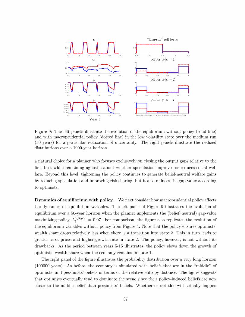
0 1 0 2 0 3 0 4 0 5 01

1 .5

2

0 1 0 2 0 3 0 4 0 5 00

0 .5

1

0 1 0 2 0 3 0 4 0 5 0

0 .91

1 .11 .21 .3

0 1 0 2 0 3 0 4 0 5 0

Y ear t

­ 0 .0 10

0 .0 10 .0 20 .0 3

0 .5 1 1 .5 2 2 .50

0 .5

1

0 0 .2 0 .4 0 .6 0 .8 10

2

4

0 0 .2 0 .4 0 .6 0 .8 10

2

4

­ 0 .0 1 5­ 0 .0 1­ 0 .0 0 5 0 0 .0 0 5 0 .0 1 0 .0 1 5 0 .0 2 0 .0 2 5 0 .0 30

5 0

Figure 9: The left panels illustrate the evolution of the equilibrium without policy (solid line)and with macroprudential policy (dotted line) in the low volatility state over the medium run(50 years) for a particular realization of uncertainty. The right panels illustrate the realizeddistributions over a 1000-year horizon.

a natural choice for a planner who focuses exclusively on closing the output gaps relative to the

first best while remaining agnostic about whether speculation improves or reduces social wel-

fare. Beyond this level, tightening the policy continues to generate belief-neutral welfare gains

by reducing speculation and improving risk sharing, but it also reduces the gap value according

to optimists.

Dynamics of equilibrium with policy. We next consider how macroprudential policy affects

the dynamics of equilibrium variables. The left panel of Figure 9 illustrates the evolution of

equilibrium over a 50-year horizon when the planner implements the (belief—neutral) gap-value

maximizing policy, λo,pl,gap1 = 0.07. For comparison, the figure also replicates the evolution of

the equilibrium variables without policy from Figure 4. Note that the policy ensures optimists’

wealth share drops relatively less when there is a transition into state 2. This in turn leads to

greater asset prices and higher growth rate in state 2. The policy, however, is not without its

drawbacks. As the period between years 5-15 illustrates, the policy slows down the growth of

optimists’wealth share when the economy remains in state 1.

The right panel of the figure illustrates the probability distribution over a very long horizon

(100000 years). As before, the economy is simulated with beliefs that are in the “middle” of

optimists’and pessimists’beliefs in terms of the relative entropy distance. The figure suggests

that optimists eventually tend to dominate the scene since their policy-induced beliefs are now

closer to the middle belief than pessimists’beliefs. Whether or not this will actually happen

37

depends on the objective belief.13 The figure also suggests that the economy spends relatively

more time in the range in which optimists’wealth share is in the intermediate range. This is

intuitive, since the policy ensures that optimists’wealth grows more slowly in state 1 but that

it is also preserved in state 2. As we argued earlier, the latter feature brings the output in state

2 closer to the first-best level, which generates a belief-neutral increase in expected gap values

(regardless of which belief dominates in the long run).

5.2.2. Macroprudential policy during the bust

The analysis so far concerns macroprudential policy in the low-volatility state and maintains

the assumption that λo,pl2 = λo2. We next consider the polar opposite case in which the planner

can reduce optimists’transition probability in the high-volatility state, λo,pl2 , while maintaining

λo,pl1 = λo1. We obtain a sharp result for the special case in which optimists’wealth share is

suffi ciently large.

Proposition 4. Consider the equilibrium with heterogeneous beliefs, together with macropru-

dential policy that satisfies λo,pl1 = λo1 (so policy affects only λo,pl2 ). Then, there exists a threshold

wealth-share level, α < 1, such that,

∂wis (α)

∂(−λo,pl2

)∣∣∣∣∣∣λo,pl=λo

< 0 for each i ∈ {o, p} , s ∈ {1, 2} and α ∈ (α, 1) .

Thus, over this range of wealth shares, macroprudential policy also reduces the planner’s value,

∂vpls (α)

∂(−λo,pl2

)∣∣∣∣∣λo,pl=λo

= ∂wpls (α)

∂(−λo,pl2

)∣∣∣∣∣λo,pl=λo

< 0.

Thus, in contrast to Proposition 3, macroprudential policy in the bust phase can actually

reduce the social welfare. To understand this result, consider the differential equation (52) for

state s = 2 and an arbitrary belief type i ∈ {o, p}. Differentiating this expression with respectto policy,

(−λo,pl2

), (since we now consider a decrease in λo,pl2 ) and evaluating at the no-policy

equilibrium, λo,pl2 = λo2, we obtain,

(ρ+ λi2

) ∂wi2 (α)

∂(−λo,pl2

) =

(1 +

ψ

ρ

)∂q2 (α)

∂(−λo,pl2

)+α (1− α)

[∂wi2 (α)

∂α− λi2

∂α′

∂λo,pl2

∂wi1 (α′)

∂α′

]+xindirect,

(55)

where α′ = aλo,pl2

λp2+α∆λpl2. Here, xindirect captures the induced effects of macroprudential policy on

the value function that typically do not drive the comparative statics. The remaining terms

capture the direct effects.

The bracketed terms in (55) are the analogues of the corresponding terms in Eq. (53). As

before, these terms capture the potential benefits of macroprudential policy from reallocating13 In any case, the long-run survival analysis does not seem practically relevant in our context. With our

simulation, pessimists do not disappear even after 100000 years.

38

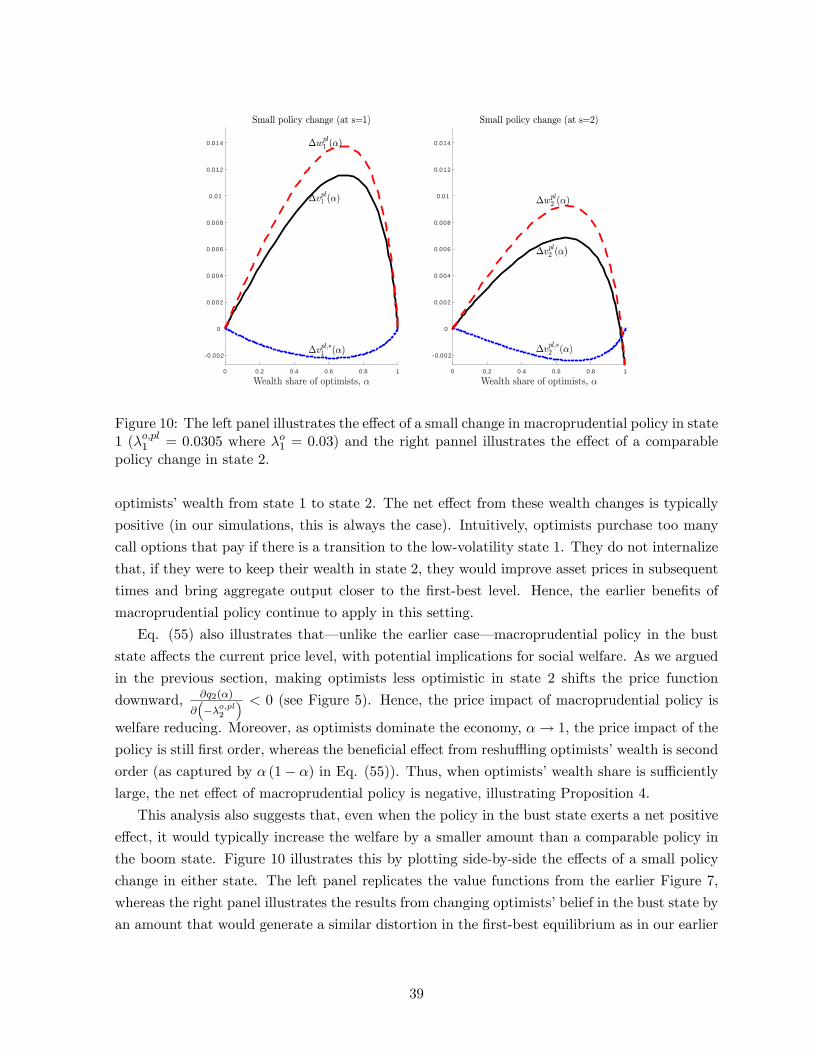
0 0.2 0.4 0.6 0.8 1

­0.002

     0

 0.002

 0.004

 0.006

 0.008

  0.01

 0.012

 0.014

0 0.2 0.4 0.6 0.8 1

­0.002

     0

 0.002

 0.004

 0.006

 0.008

  0.01

 0.012

 0.014

Figure 10: The left panel illustrates the effect of a small change in macroprudential policy in state1 (λo,pl1 = 0.0305 where λo1 = 0.03) and the right pannel illustrates the effect of a comparablepolicy change in state 2.

optimists’wealth from state 1 to state 2. The net effect from these wealth changes is typically

positive (in our simulations, this is always the case). Intuitively, optimists purchase too many

call options that pay if there is a transition to the low-volatility state 1. They do not internalize

that, if they were to keep their wealth in state 2, they would improve asset prices in subsequent

times and bring aggregate output closer to the first-best level. Hence, the earlier benefits of

macroprudential policy continue to apply in this setting.

Eq. (55) also illustrates that– unlike the earlier case– macroprudential policy in the bust

state affects the current price level, with potential implications for social welfare. As we argued

in the previous section, making optimists less optimistic in state 2 shifts the price function

downward, ∂q2(α)

∂(−λo,pl2

) < 0 (see Figure 5). Hence, the price impact of macroprudential policy is

welfare reducing. Moreover, as optimists dominate the economy, α→ 1, the price impact of the

policy is still first order, whereas the beneficial effect from reshuffl ing optimists’wealth is second

order (as captured by α (1− α) in Eq. (55)). Thus, when optimists’wealth share is suffi ciently

large, the net effect of macroprudential policy is negative, illustrating Proposition 4.

This analysis also suggests that, even when the policy in the bust state exerts a net positive

effect, it would typically increase the welfare by a smaller amount than a comparable policy in

the boom state. Figure 10 illustrates this by plotting side-by-side the effects of a small policy

change in either state. The left panel replicates the value functions from the earlier Figure 7,

whereas the right panel illustrates the results from changing optimists’belief in the bust state by

an amount that would generate a similar distortion in the first-best equilibrium as in our earlier

39

analysis.14 Note that a small macroprudential policy in state 2 has a smaller positive impact

when optimists’wealth share is small, and it has a negative impact when optimists’wealth share

is suffi ciently large.

It is useful to emphasize that macroprudential policy does not have an adverse price impact

in the boom state due to the interest rate response. As we argued in the previous section,

reducing optimists’optimism in state 1 leaves the price level unchanged at q1 (α) = q∗, but it

shifts the interest rate function downward (see Figure 5). Intuitively, as macroprudential policy

reduces the demand for risky assets, the interest rate policy lowers the rate to dampen its effect

on asset prices and aggregate demand. In state 2, the interest rate is already at zero, so the

interest rate policy cannot neutralize the adverse effects of macroprudential policy.

Taken together, our analysis in this section provides support for procyclical macroprudential

policy. In states in which output is not demand constrained (in our model, state 1), macro-

prudential policy that restricts high valuation investors’(in our model optimists’) risk taking

is desirable. This policy improves welfare by ensuring that high valuation investors bring more

wealth to the demand-constrained states, which in turn increases asset prices and output. Its

adverse price effects are countered by a reduction in the interest rate. In contrast, in states in

which output is demand constrained (in our model, state 2), macroprudential policy has coun-

teracting effects on social welfare. While the policy has the same beneficial effects as before,

it also lowers asset prices and aggregate demand, which cannot be countered by the interest

rate. The latter effect reduces the overall usefulness of macroprudential policy, and it could even

reduce social welfare.

6. Forward guidance

Macroprudential policy reduces the perverse interactions between speculation and interest-rate

constraints, but it does not relax the latter. We next consider the possibility of forward-guidance

type policies that lower interest rates in the future to stimulate aggregate output in earlier

periods. Formally, we drop the policy rule in (18) and allow the planner to commit to setting

an interest rate path subject to the lower bound constraint, (17), as well as the remaining

equilibrium conditions.

To allow forward guidance to stimulate the economy, we let factor utilization, ηt,s, exceed one.

However, excess utilization is costly and induces a faster depreciation of capital. In particular,

we now replace the capital evolution equation (1) with

dkt,skt,s

=(ϕ (ιt,s)− δ

(ηt,s))dt+ σsdZt, where δ

(ηt,s)

= δ + δη max(0, ηt,s − 1

).

Here, δη (η − 1) captures the additional depreciation rate caused by overutilization (which we

14Specifically, we calibrate the belief change in state 2 so that the maximum decline in the planner’s first-best

value function is the same in both cases, maxα

∣∣∣∆vpl,∗2 (α)∣∣∣ = maxα

∣∣∣∆vpl,∗1 (α)∣∣∣.

40

take to be a linear function of η for simplicity). Appendix A.4.1 describes the remaining changes

we make to the New Keynesian supply block of the model to accommodate excess factor utiliza-

tion. With appropriate assumptions, equations (15) and (16) continue to apply in this setting:

that is, output is determined by aggregate demand, and the rental rate of capital (which now

also includes the overutilization costs) ensures all output accrues to the agents in the form of

return to capital.

We also focus on the benchmark model without disagreement and with two states developed

in Section 3, with three additional assumptions. First, for analytical tractability, we assume

the planner sets policies within a restricted class. We start by analyzing the case in which the

planner is restricted to set a fixed level of interest rate for each state, rfs , and to implement a

fixed level of factor utilization, ηs. Second, we assume the parameters satisfy the following.

Assumption 5. δη exp (q∗) > A (ρψ + 1) (where exp (q∗) = A+ψρ+ψ ).

This condition says the marginal loss of value from excess depreciation is greater than the

marginal gain of value from increasing factor utilization beyond η1 = 1. It ensures that, in the

first-best benchmark without interest rate rigidities, the planner would not implement excess

factor utilization (see Appendix A.4.2). Third, we also restrict attention to the case in which

there is no investment, ψ = 0, which leads to particularly simple expressions. The case with

ψ > 0 generates qualitatively similar results.

With these assumptions, it easy to see that the goods market equilibrium condition (19)

continues to hold in the high-volatility state s = 2, but it is modified in the low-volatility

state s = 1. We first characterize the equilibrium given a particular forward guidance policy,(rf1 , η1 ≥ 1

), and illustrate that our model generates a version of the forward guidance puzzle.

We then characterize the (constrained) optimal policy.

Effectiveness of forward guidance. As before, there is an increasing relationship between

asset prices and factor utilization (cf. Eq. (22)),

q1 = q (η1) ≡ log

(Aη1

ρ

).

This illustrates that providing greater stimulus in state 1 also increases the asset price in that

state. Applying the risk balance condition (26) for state s = 1, we obtain,

rf1 = ρ− δ + λ1 (1− exp (q (η1)− q2))− δη (η1 − 1)− σ21 ≥ 0, (56)

as long as η1 ≥ 1. This illustrates that providing greater stimulus in state s = 1 requires setting

a lower interest rate. Likewise, using the condition for state s = 2, we obtain,

rf2 = ρ− δ + λ2 (1− exp (q2 − q (η1)))− σ22 = 0, (57)

41

as long as q2 ≤ q∗. This illustrates that providing greater stimulus in state 1 also increases the

asset price in state 2 by increasing the expected capital gains.

Given some η1 ≥ 1, the equilibrium pair,(rf1 , q2

)(with q2 ≤ q∗2), is characterized as the

solution to Eqs. (56) and (57). Note also that, applying these equations for η1 = 1 results in the

benchmark equilibrium described in Section 3, which we denote by(rf,b1 , qb1, q

b2

). Using these

benchmark variables, Eqs. (56) and (57) can be respectively replaced with

rf1 = rf,b1 − δη (η1 − 1) ,

q2 = q (η1) + qb2 − qb1.

The planner can then be thought of as targeting some η1 ≥ 1, which requires setting the interest

rate according to the first equation, and which determines the asset prices according to the

second equation.

A surprising aspect of the equilibrium is that the prices in both states move in tandem

regardless of transition probabilities. For instance, when state 2 is persistent (low λ2), one could

have expected the forward guidance policy that affects the outcomes in state 1 to have a small

impact on q2. Eq. (57) illustrates that this is not the case: forward guidance policy that

increases q1 (η1) by some amount also increases q2 by the same amount.

This is a manifestation of the “forward guidance puzzle”: the phenomenon that, in standard

New Keynesian models, interest rate announcements far in the future have large effects on

current output as well as inflation (see, for instance, Del Negro et al. (2012); McKay et al.

(2016); Werning (2015)). The puzzle obtains largely because of strong general equilibrium

effects. Specifically, interest rate cuts in the distant future increase output in future periods.

These output increases are anticipated by economic agents, which then increases output also

in the current period. Our model is slightly different than the models analyzed by the recent

literature since the transition out of the liquidity trap is probabilistic as opposed to deterministic.

Nonetheless, the model features strong general equilibrium effects that lead to a similar forward

guidance puzzle.

To illustrate the role of future policy commitments (and the associated general equilibrium

effects), consider the following alternative policy exercise in which the strength of the policy is

decreasing in the amount of time the economy spends in state s = 2 before transitioning into

state s = 1. For concreteness, let t denote the time spent in state 2, and suppose the planner im-

plements an after-transition price level, q1 (t), that satisfies, q1 (t)− qb1 = exp (−ζt)(q1 (0)− qb1

),

for some q1 (0) ≥ qb1 and ζ ≥ 0. Once implemented, the price in state 1 is kept constant at q1 (t)

until a further state transition. The parameter, ζ, captures the rate at which the strength of the

policy declines as state 2 persists longer. The earlier analysis is a special case with q1 (0) = q (η1)

and ζ = 0. When ζ > 0, the equilibrium condition (57) is replaced with,

ρ− δ + λ2 (1− exp (q2 (t)− q1 (t))) +dq2 (t)

dt− σ2

2 = 0. (58)

42

0 2 4 6 8 10

0.82

0.84

0.86

0.88

0.9

0.92

0.94

0.96

0.98

1

1.02

0 2 4 6 8 10

0.82

0.84

0.86

0.88

0.9

0.92

0.94

0.96

0.98

1

1.02

Figure 11: The effects of foward guidance policy on prices when investors are pessimistic (leftpanel) and optimistic (right panel), and when the policy is persistent (solid lines) and somewhattransient (dashed lines). When we change λ2, we also change σ2, so as to keep the benchmakprice level, qb2, constant across policy exercises.

The equilibrium price function, q2 (t), solves this differential equation with the limit condition,

limt→∞ q2 (t) = qb2.

The left panel of Figure 11 illustrates the solution for different levels of ζ when investors are

pessimistic (low λ2). The solid lines illustrate the earlier results with persistent policy, ζ = 0.

Note that the policy increases q1 (t) and q2 (t) by the same amount. We chose q1 (0) suffi ciently

high so that the policy completely eliminates the recession in the high volatility state, q2 (0) = q∗.

The dashed lines illustrate the same example with slightly less persistent policy, ζ = 0.1. In this

case, q2 (0) barely moves relative to its benchmark level, qb2. The intuition comes from inspecting

Eq. (58). Conditional on there not being a transition, there will be a downward drift in prices as

the policy will have weaker effects in the future, dq2(t)dt < 0. This downward drift is recognized by

all investors and reduces the price also in earlier periods. This illustrates that, when investors

are pessimistic, forward guidance increases the price largely because of its stimulative effects in

future periods.

The right panel of Figure 11 repeats the same exercise when investors are optimistic (high

λ2). We also adjust the volatility parameter, σ2, to ensure that the benchmark price, qb2, is the

same as before (despite greater optimism). In this case, the policy generates a sizeable increase

in q2 (0) even when it is not very persistent. This illustrates that, when investors are optimistic,

forward guidance policy relies much less on affecting the outcomes in the distant future. Rather,

forward guidance in this case operates more directly by generating capital gains conditional on

there being a transition in the near future.

43

These results relate to a growing literature that proposes to resolve the forward guidance

puzzle by weakening the general equilibrium effects that obtain in the distant future. For in-

stance, Angeletos and Lian (2016) illustrate that, when the policy is not common knowledge, the

effectiveness of the forward policy declines with the time-horizon (since the general equilibrium

effects rely on higher order beliefs). Farhi and Werning (2016a) illustrate that a similar outcome

obtains when investors are boundedly rational (with level-k thinking) and the financial markets

are incomplete. Gabaix (2017) obtains a related result by assuming that agents are inattentive

to future changes to interest rates. While our model does not feature these ingredients, our

analysis suggests that these types of frictions that weaken the effectiveness of policy in future

periods have a stronger bite when investors are pessimistic about the transition probability.

With optimism, there is scope for forward guidance policy even if the agents discount its effects

in future periods.15

Optimal forward guidance. We next turn to the characterization of the (constrained) opti-

mal forward guidance policy. For simplicity, consider the baseline case with ζ = 0 so the planner

chooses a time-invariant policy. Suppose the economy starts in state s = 2 and the planner

chooses the policy,(rf1 , η1

), to maximize the welfare of the representative household in this

state, v2. Following the same steps as in Section 3, and using ψ = 0, the value function in state

2 is given by,

ρv2 = log ρ+ β2

(1

ρq2 −

1

ρδ

)+ (1− β2)

(1

ρq (η1)− 1

ρδ (η1)

)− 1

ρσ2

2, (59)

where β2 =ρ+ λ1

ρ+ λ1 + λ2.

As before, β2 denotes the amount of discounting-adjusted time the economy spends in state

2. The main difference from Section 3 is that the depreciation rate in state 1 is replaced with

δ (η1) = δ + δη (η1 − 1).

The planner effectively chooses η1 ≥ 1 to maximize Eq. (59) subject to the pricing relation,

q2 = q (η1) + qb2 − qb1, and the inequality constraints q2 ≤ q∗ and rf1 ≥ 0. Using the first order

conditions, the planner utilizes some forward guidance (η1 > 1) if and only if

∆q ≡ log

(1

1− β2

ρ

δη

)> 0. (60)

This expression illustrates that forward guidance is more likely to be utilized when it is cheaper

(low δη), and when the current high-volatility state is likely to persist (high β2). In the extreme

case in which the high-volatility state is very transient, β2 = 0, Assumption 5 implies that

forward guidance is not used. In the other extreme in which the current state is very persistent,

15This discussion also connects with Caballero and Farhi (2017), who illustrate how forward guidance losseseffectiveness in liquidity traps caused by an scarcity of safe assets. In their model, the marginal agent is concernedwith further negative shocks and ascribes little value to promises to be delivered in better states of the world.

44

β2 → 1, the forward guidance is always used. It is also easy to check that, when condition (60)

holds and there is an interior solution, the optimal forward guidance policy stimulates the prices

by exactly ∆q, that is, the equilibrium features q1 − qb1 = q2 − qb2 = ∆q. If there is a corner

solution, then the equilibrium with optimal policy features either qb2 = q∗ or rf1 = 0.

Note that the persistence parameter, β2, is inversely related to the transition probability, λ2.

Hence, our analysis in this section suggests a tension in the determination of the optimal forward

guidance policy. If investors are rationally optimistic, then forward guidance is not particularly

desirable (since the recovery is imminent). However, if the policy becomes weaker with time

horizon (perhaps due to the frictions emphasized by the recent literature), then optimism also

increases the effectiveness of the policy. Hence, whether optimism increases or decreases the

optimal provision of forward guidance is ambiguous and it is likely to depend on the details of

the setting.

7. Endogenous Volatility and Incomplete Markets

So far, we emphasized how the interest rate rigidities, combined with risk premium shocks,

can push the economy into a demand-driven recession, and how speculation exacerbates the

recession. In this section, we illustrate how the interest rate rigidities and speculation can also

generate endogenous volatility in asset prices. In our model, there is endogenous volatility even

in the homogeneous beliefs benchmark, but the effects become particularly salient when investors

speculate on their heterogeneous beliefs and their wealth shares fluctuate within each state due

to incomplete markets. We develop this argument in two steps, first within the homogenous

beliefs benchmark, and then within an extension of the framework to the incomplete markets

case. The latter also helps to connect our framework to the related macrofinance literature

summarized in Brunnermeier and Sannikov (2016b)

7.1. Endogenous Volatility from Interest Rate Rigidities

Given some ∆t > 0, we define the proportional change in aggregate wealth over this time interval

as,∆kt,sQt,s/∆t

kt,sQt,s≡ (kt+∆t,sQt+∆t,s − kt,sQt,s) /∆t

kt,sQt,s.

We will characterize the instantaneous volatility of this expression. First consider the homoge-

nous belief benchmark that we analyzed in Section 3. In this model, while the instantaneous

volatility conditional on there being no transition is exogenous (given by σs), the unconditional

volatility that also incorporates the jump risk in asset prices is endogenous. In Appendix B, we

show that the instantaneous variance is given by,

lim∆t→0

V art,s

(∆kt,sQt,s/∆t

kt,sQt,s

)= σ2

s +∑s′ 6=s

λs,s′

(Qs′ −Qs

Qs

)2

. (61)

45

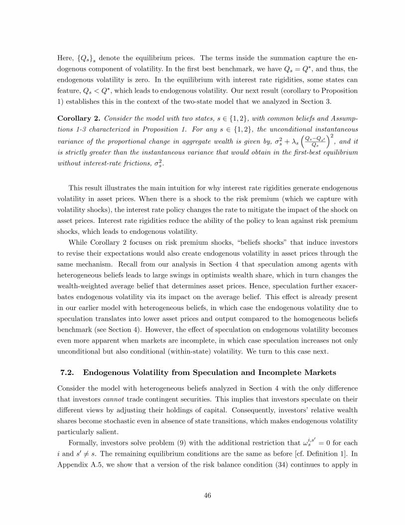
Here, {Qs}s denote the equilibrium prices. The terms inside the summation capture the en-

dogenous component of volatility. In the first best benchmark, we have Qs = Q∗, and thus, the

endogenous volatility is zero. In the equilibrium with interest rate rigidities, some states can

feature, Qs < Q∗, which leads to endogenous volatility. Our next result (corollary to Proposition

1) establishes this in the context of the two-state model that we analyzed in Section 3.

Corollary 2. Consider the model with two states, s ∈ {1, 2}, with common beliefs and Assump-tions 1-3 characterized in Proposition 1. For any s ∈ {1, 2}, the unconditional instantaneousvariance of the proportional change in aggregate wealth is given by, σ2

s + λs

(Qs−Qs′Qs

)2, and it

is strictly greater than the instantaneous variance that would obtain in the first-best equilibrium

without interest-rate frictions, σ2s.

This result illustrates the main intuition for why interest rate rigidities generate endogenous

volatility in asset prices. When there is a shock to the risk premium (which we capture with

volatility shocks), the interest rate policy changes the rate to mitigate the impact of the shock on

asset prices. Interest rate rigidities reduce the ability of the policy to lean against risk premium

shocks, which leads to endogenous volatility.

While Corollary 2 focuses on risk premium shocks, “beliefs shocks” that induce investors

to revise their expectations would also create endogenous volatility in asset prices through the

same mechanism. Recall from our analysis in Section 4 that speculation among agents with

heterogeneous beliefs leads to large swings in optimists wealth share, which in turn changes the

wealth-weighted average belief that determines asset prices. Hence, speculation further exacer-

bates endogenous volatility via its impact on the average belief. This effect is already present

in our earlier model with heterogeneous beliefs, in which case the endogenous volatility due to

speculation translates into lower asset prices and output compared to the homogeneous beliefs

benchmark (see Section 4). However, the effect of speculation on endogenous volatility becomes

even more apparent when markets are incomplete, in which case speculation increases not only

unconditional but also conditional (within-state) volatility. We turn to this case next.

7.2. Endogenous Volatility from Speculation and Incomplete Markets

Consider the model with heterogeneous beliefs analyzed in Section 4 with the only difference

that investors cannot trade contingent securities. This implies that investors speculate on their

different views by adjusting their holdings of capital. Consequently, investors’relative wealth

shares become stochastic even in absence of state transitions, which makes endogenous volatility

particularly salient.

Formally, investors solve problem (9) with the additional restriction that ωi,s′

s = 0 for each

i and s′ 6= s. The remaining equilibrium conditions are the same as before [cf. Definition 1]. In

Appendix A.5, we show that a version of the risk balance condition (34) continues to apply in

46

this case,

σs + σQt,s =1

σs + σQt,s

rkt,s − rft,s +∑s′ 6=s

λis,s′

({ωk,it,2

}i

) Qt,s′ −Qt,sQt,s′

, (62)

where λs,s′({ωk,it,2

}i

)=

∑i

αit,sχ(ωk,it,s

)λis,s′ and χ

(ωk,it,s

)=

Qt,s′

Qt,s + ωk,it,s(Qt,s′ −Qt,s

) .As before, capital is priced according to an appropriately weighted average belief. The weights

incorporate the fact that investors might have different marginal utilities after a jump since

they place different portfolio weights on capital, that is, ωk,it,s is not necessarily equal to one. In

particular, investors’portfolio weights are characterized by jointly solving the following system

of equations (over i ∈ I),

(ωk,it,s − 1

)(σs + σQt,s

)=

1

σs + σQt,s

∑s′ 6=s

(λis,s′χ

(ωk,it,s

)− λ2

({ωk,it,2

}i

))(Qt,s′ −Qt,sQt,s′

). (63)

Note that the investor holds more capital (ωk,it,s > 1), if she is optimistic about the expected

capital gains relative to the weighted average belief. Unlike in Section 4, investors speculate

on their different beliefs about transition probabilities by adjusting their portfolio weights on

capital. Note also that, since capital is the only available risky investment, ωk,it,s provides a

measure of the investor’s leverage ratio: the value of her risky assets divided by the value of her

wealth.

To characterize the equilibrium further, consider the two-state special case. As before, we

conjecture an equilibrium in which the prices and interest rates satisfy, qt,1 = q∗, rft,1 > 0 and

qt,2 < q∗, rft,2 = 0. Moreover, the price in state 2 can be written as a function of optimists’

wealth share, qt,2 = q2 (αt,2) for some function q2 : [0, 1]→ [qp2 , qo2]. Likewise, the interest-rate in

state 1 can be written as a function of optimists’wealth share, r1 (αt,1). We next characterize

the equilibrium in state s = 2. The equilibrium in state s = 1 is characterized by similar steps.

Appendix A.5 shows that applying Eq. (63) in this case implies ωk,ot,2 > 1 > ωk,pt,2 : that

is, optimists’leverage ratio exceeds one. Intuitively, optimists make a leveraged investment in

capital since they assign a greater probability to transition into state s = 1 (that features higher

asset prices). In view of their leveraged exposure to capital, optimists’wealth share fluctuates

even without any state transition. In Appendix A.5, we show that within a state optimists’

wealth share evolves according to,

dαt,2αt,2

=(ωk,ot,2 − 1

)(rkt,2 −

(σ2 + σQt,2

)2)dt+

(ωk,ot,2 − 1

)(σ2 + σQt,2

)dZt, (64)

where rkt,2 is given by Eq. (24) as before. Note that (since ωk,ot,2 > 1) a negative shock to the

Brownian motion, dZt < 0, decreases optimists’wealth share. Since the asset price is a function

47

0 0.2 0.4 0.6 0.8 1

0.85

0.9

0.95

1

1.05

1.1

1.15

1.2

1.25

1.3

0 0.2 0.4 0.6 0.8 10.315

0.32

0.325

0.33

0.335

0.34

0.345

0.35

0.355

0.36

0 0.2 0.4 0.6 0.8 1­18

­16

­14

­12

­10

­8

­6

­4

­2

0

2 10 ­3

0 0.2 0.4 0.6 0.8 11

1.1

1.2

1.3

1.4

1.5

1.6

1.7

1.8

1.9

Incomplete markets Complete markets

Figure 12: The solid lines (resp. the dashed) lines illustrate the equilibrium in state 2 withincomplete markets (resp. complete markets).

of optimists’wealth share, qt,2 = q2 (αt,2), these changes also translate into fluctuations in the

asset price. In particular, the endogenous volatility term, σQt,2, is no longer zero and it is solved

as part of the equilibrium.

Formally, our analysis in Appendix A.5 shows that Eq. (64) describes the drift and the

volatility of asset prices, µQt,2 and σQt,2, in terms of the price function as well as its derivatives,

q2 (α) , q′2 (α) , q′′2 (α). Combining these expressions with the risk balance condition (62) for state

s = 2 provides a second order ordinary differential equation for the price function, q2 (α). The

equilibrium is the solution to this differential equation together with the boundary conditions,

q2 (0) = qp2 and q2 (1) = qo2, as well as q′2 (0) (that we characterize in the appendix).

Figure 3 illustrates the equilibrium for the particular parameterization we analyzed in Section

4. The solid lines plot the equilibrium variables with incomplete markets, and the dashed lines

48

plot the corresponding variables with complete markets. The top left panel shows that, as

before, the price function is increasing in optimists’wealth share. Less obviously, the figure also

illustrates that the price is greater than in the complete markets case. The bottom left panel

shows that this outcome obtains because the complete markets case features a more negative

price drift. Intuitively, completing the market (by adding the contingent securities) increases

the scope for speculation, which implies that optimists’wealth share declines by more when the

high-volatility state persists longer. This effect is related to the results in Simsek (2013b), which

illustrate that financial innovation (that expands the set of traded financial assets) can increase

investors’portfolio risks in view of greater speculation. In our model, greater portfolio risks

translate into greater (unconditional) endogenous volatility, which in turn reduces asset prices

and output during a demand recession.

The top right panel shows that, although the price level is higher, within-state volatility of

capital is also higher in this case in view of the endogenous price volatility, σQt,2. The bottom

right panel shows that this outcome obtains because optimists’leverage ratio exceeds one. The

figure also illustrates that optimists’leverage ratio is greater when their wealth share is lower, as

this leads to lower asset prices and greater capital gains from a transition into state s = 1, which

optimists find more likely. Note also that σQt,2 obtains its highest level for an intermediate level

of optimists’wealth share, αt,2. This result can be understood from Eq. (64), which illustrates

that the magnitude of the fluctuations in αt,2 (that determines the price level, q2 (αt,2)) is

determined by the product of optimists’ leverage ratio and the current level of their wealth

share,(ωk,ot,2 − 1

)αt,2. Intuitively, speculation is stronger, and leads to greater endogenous

volatility, when both types of investors have a sizeable wealth share.

8. Final Remarks

We provide a macroeconomic framework where risk- and output—gaps are joint phenomena that

feed into each other. The key tension in this framework is that asset prices have the dual role of

equilibrating risk markets and supporting aggregate demand. When the dual role is inconsistent,

the risk market equilibrium prevails. Interest rate policy works by taking over the role of

equilibrating risk markets, which then leaves asset prices free to balance the goods markets.

However, once interest rates reach a lower bound, the dual role problem reemerges and asset

prices are driven primarily by risk markets equilibrium considerations. This reduces aggregate

demand and triggers a recession, which then feeds back negatively into asset prices. The role

of macroprudential regulation is to reduce the gap between the asset prices that equilibrate the

risk and goods markets when interest rate policy is no longer available.

Interest rate cuts work in our model by improving the market’s Sharpe ratio. From this

perspective, any policy that reduces market volatility should have similar effects, which renders

support to the many such policies implemented during the aftermath of the subprime and

European crises. And it is also reasonable to expect that, over time and should the high risk-

49

awareness environment persist, the private sector may migrate to safer technologies and sectors,

at the cost of lower growth. We are exploring these implications in concurrent work.

In the model we take the interest rate friction to be a stark zero lower bound constraint,

which can be motivated with standard cash-substitutability arguments. In practice, this con-

straint is neither as tight nor as narrowly motivated: Central banks do have some space to bring

rates into negative territory, especially when macroeconomic uncertainty is rampant, but there

are also many other frictions besides cash substitutability that can motivate downward rigidity

in rates once these are already low (see, e.g., Brunnermeier and Koby (2016) for a discussion of

the “reversal rate”, understood as a level of rates below which the financial system becomes im-

paired). The broader points of the dual role of asset prices and their interactions with aggregate

demand constraints during recessions would survive many generalizations of the interest rate

friction. Similarly, and as we hinted in the Forward Guidance section of the paper, one could

also imagine situations that motivate ceilings on interest rates, in which case asset prices would

overshoot and the productive capacity would become stretched.

We also chose to narrate the interactions between speculation and aggregate demand in terms

of the economy’s degree of optimism. Naturally, there is an entirely symmetric discussion in

terms of the economy’s degree of pessimism, in which case our paper connects with the literature

that ascribes the depth of risk-based crises to Knightian uncertainty (see, e.g., Caballero and

Krishnamurthy (2008); Caballero and Simsek (2013)). However, absent any direct mechanism

to alleviate Knightian behavior during severe recessions, the key macroprudential point that

optimists may need to be regulated during the boom survives this alternative motivation.

We deliberately kept our analysis of heterogeneity in asset valuation at an abstract level.

With this ingredient our goal was to highlight the negative effect of (ex-ante) speculation on

(ex-post) aggregate demand and growth. During booms, speculation boosts valuations and

aggregate demand, but these effects can be offset by higher rates. In contrast, during severe

recessions, speculation depresses valuations and aggregate demand, but these effects cannot be

offset by interest rates cuts as these are constrained. In practice, this insight implies that (from

a macroeconomic point of view) it doesn’t matter whether banks are the optimists or pessimists:

If the former, then their leverage during the boom (selling puts) is costly during recessions as

they become impaired; if the latter, then their (fully collateralized) easy lending during booms

(buying puts) implies that their optimistic borrowers will suffer losses during recessions.

As we noted earlier, our modeling approach belongs to the literature spurred by Brunnermeier

and Sannikov (2014), although unlike that literature most of our analysis does not feature

financial frictions. However, if we were to introduce these realistic frictions in our setting, many

of the themes in that literature would reemerge and become exacerbated by aggregate demand

feedbacks. For instance, as we show in Section 7.2 in an incomplete markets setting, optimists

take leveraged positions on capital, and by doing so they induce endogenous volatility in asset

prices and the possibility of tail events following a sequence of negative diffusion shocks that

make the economy deeply pessimistic.

50

The model omits many realistic self-healing shocks that were arguably relevant for the Great

Recession (as well as other deep recessions). For example, a financial crisis driven by a reduction

in banks’net worth is typically mitigated over time as banks earn high returns and accumulate

net worth (see Gertler et al. (2010); Brunnermeier and Sannikov (2014)). Likewise, household or

firm deleveraging eventually loses its potency as debt is paid back (see Eggertsson and Krugman

(2012); Guerrieri and Lorenzoni (2017)). Investment hangovers gradually dissipate as the excess

capital is depleted (see Rognlie et al. (2017)). While these self-healing shocks are useful to

understand the depth of the Great Recession, they raise the natural question of why the interest

rates seem unusually low and the recovery (especially in investment) appears incomplete almost

ten years after the start of the recession. Our paper illustrates how (objective and subjective)

risk factors can drag the economy’s recovery.

Conversely, the model also omits many sources of inertia that stem from financial markets.

Throughout we have assumed that risk-markets clear instantly while goods markets are sluggish.

In practice, risk-market have their own sources of inertia as financial institutions avoid or delay

mark-to-market losses, liquidity evaporates, policy noise rises, and so on.

Finally, one feature of the aftermath of the subprime crisis is the present high valuation of

risk-assets, that could appear to contradict the higher required equity risk premium observed

in the data (see Figure 1). The model offers a natural interpretation for such a combination:

While we focused exclusively on changes in the required risk-premium, there is also evidence

that during this period both ρ and ψ have declined due to a variety of factors such as a worsening

of the income distribution and an increase in monopoly rents (see, e.g., Gutiérrez and Philippon

(2016)). Equation (22) shows that such declines require a higher valuation for any given level

of output gap η, which is achieved via a drop in “rstar.”In the interest rate constrained region

the latter translates into a deeper recession, while once the economy has recovered the decline

in“rstar”manifests in lower riskless interest rates and higher valuations. It may well be that

this new high valuation full-employment equilibrium will bring about higher instability in the

future by exacerbating speculation, which is a theme we intend to explore in future work.

References

Adrian, T., Boyarchenko, N., 2012. Intermediary leverage cycles and financial stability.

Angeletos, G.-M., Lian, C., 2016. Forward guidance without common knowledge. Tech. rep., National

Bureau of Economic Research.

Bacchetta, P., Benhima, K., Kalantzis, Y., 2016. Money and capital in a persistent liquidity trap.

Basak, S., 2000. A model of dynamic equilibrium asset pricing with heterogeneous beliefs and extraneous

risk. Journal of Economic Dynamics and Control 24 (1), 63—95.

Basak, S., 2005. Asset pricing with heterogeneous beliefs. Journal of Banking & Finance 29 (11), 2849—

2881.

51

Basak, S., Cuoco, D., 1998. An equilibrium model with restricted stock market participation. Review of

Financial Studies 11 (2), 309—341.

Bernanke, B. S., Gertler, M., Gilchrist, S., 1999. The financial accelerator in a quantitative business cycle

framework. Handbook of macroeconomics 1, 1341—1393.

Bianchi, J., Mendoza, E. G., 2013. Optimal time-consistent macroprudential policy. Tech. rep., National

Bureau of Economic Research.

Bloom, N., 2009. The impact of uncertainty shocks. econometrica 77 (3), 623—685.

Brunnermeier, M. K., Koby, Y., 2016. The reversal interest rate: An effective lower bound on monetary

policy. Preparation). Print.

Brunnermeier, M. K., Sannikov, Y., 2014. A macroeconomic model with a financial sector. The American

Economic Review 104 (2), 379—421.

Brunnermeier, M. K., Sannikov, Y., 2016a. The i theory of money. Tech. rep., National Bureau of Eco-

nomic Research.

Brunnermeier, M. K., Sannikov, Y., 2016b. Macro, money, and finance: A continuous-time approach.

Handbook of Macroeconomics 2, 1497—1545.

Brunnermeier, M. K., Simsek, A., Xiong, W., 2014. A welfare criterion for models with distorted beliefs.

The Quarterly Journal of Economics 129 (4), 1753—1797.

Caballero, R. J., Farhi, E., 2017. The safety trap. Review of Economic Studies forthcoming.

Caballero, R. J., Farhi, E., Gourinchas, P.-O., 2017a. Rents, technical change, and risk premia accounting

for secular trends in interest rates, returns on capital, earning yields, and factor shares. American

Economic Review 107 (5), 614—620.

Caballero, R. J., Farhi, E., Gourinchas, P.-O., 2017b. The safe asset shortage conundrum. The Journal

of Economic Perspectives 31 (3).

Caballero, R. J., Krishnamurthy, A., 2003. Excessive dollar debt: Financial development and underin-

surance. The Journal of Finance 58 (2), 867—894.

Caballero, R. J., Krishnamurthy, A., 2008. Collective risk management in a flight to quality episode. The

Journal of Finance 63 (5), 2195—2230.

Caballero, R. J., Simsek, A., 2013. Fire sales in a model of complexity. The Journal of Finance 68 (6),

2549—2587.

Chen, J., Hong, H., Stein, J. C., 2002. Breadth of ownership and stock returns. Journal of financial

Economics 66 (2), 171—205.

Christiano, L. J., Eichenbaum, M. S., Trabandt, M., 2015. Understanding the great recession. American

Economic Journal: Macroeconomics 7 (1), 110—167.

52

Christiano, L. J., Motto, R., Rostagno, M., 2014. Risk shocks. The American Economic Review 104 (1),

27—65.

Curdia, V., Woodford, M., 2010. Credit spreads and monetary policy. Journal of Money, Credit and

Banking 42 (s1), 3—35.

Davila, E., Korinek, A., 2016. Pecuniary externalities in economies with financial frictions. The Review

of Economic Studies.

Del Negro, M., Giannone, D., Giannoni, M. P., Tambalotti, A., Wu, J. C., 2017. Safety, liquidity, and

the natural rate of interest.

Del Negro, M., Giannoni, M. P., Patterson, C., 2012. The forward guidance puzzle.

Detemple, J., Murthy, S., 1994. Intertemporal asset pricing with heterogeneous beliefs. Journal of Eco-

nomic Theory 62 (2), 294—320.

Di Tella, S., 2012. Uncertainty shocks and balance sheet recessions. Job Market Paper.

Eggertsson, G. B., Krugman, P., 2012. Debt, deleveraging, and the liquidity trap: A fisher-minsky-koo

approach. The Quarterly Journal of Economics 127 (3), 1469—1513.

Eggertsson, G. B., Mehrotra, N. R., Robbins, J. A., January 2017. A model of secular stagnation: Theory

and quantitative evaluation. Working Paper 23093, National Bureau of Economic Research.

URL http://www.nber.org/papers/w23093

Eggertsson, G. B., Woodford, M., September 2006. Optimal Monetary and Fiscal Policy in a Liquidity

Trap. The MIT Press, pp. 75—144.

URL http://www.nber.org/chapters/c0076

Farhi, E., Werning, I., 2016a. The power of forward guidance with bounded rationality and incomplete

markets.

Farhi, E., Werning, I., 2016b. A theory of macroprudential policies in the presence of nominal rigidities.

Econometrica 84 (5), 1645—1704.

Farhi, E., Werning, I., 2017. Fiscal unions. American Economic Review forthcoming.

Fostel, A., Geanakoplos, J., 2008. Leverage cycles and the anxious economy. The American Economic

Review 98 (4), 1211—1244.

Gabaix, X., 2017. A behavioral new keynesian model. Tech. rep., National Bureau of Economic Research.

Geanakoplos, J., 2010. The leverage cycle. NBER macroeconomics annual 24 (1), 1—66.

Gertler, M., Karadi, P., 2011. A model of unconventional monetary policy. Journal of monetary Economics

58 (1), 17—34.

Gertler, M., Kiyotaki, N., et al., 2010. Financial intermediation and credit policy in business cycle analysis.

Handbook of monetary economics 3 (3), 547—599.

53

Gilchrist, S., Zakrajšek, E., 2012. Credit spreads and business cycle fluctuations. The American Economic

Review 102 (4), 1692—1720.

Guerrieri, V., Lorenzoni, G., 2017. Credit crises, precautionary savings, and the liquidity trap. Quarterly

Journal of Economics forthcoming.

Gutiérrez, G., Philippon, T., 2016. Investment-less growth: An empirical investigation. Tech. rep., Na-

tional Bureau of Economic Research.

Hall, R. E., 2011. The long slump. The American Economic Review 101 (2), 431—469.

Harris, M., Raviv, A., 1993. Differences of opinion make a horse race. Review of Financial studies 6 (3),

473—506.

Harrison, J. M., Kreps, D. M., 1978. Speculative investor behavior in a stock market with heterogeneous

expectations. The Quarterly Journal of Economics 92 (2), 323—336.

He, Z., Krishnamurthy, A., 2012. A model of capital and crises. The Review of Economic Studies 79 (2),

735—777.

He, Z., Krishnamurthy, A., 2013. Intermediary asset pricing. The American Economic Review 103 (2),

732—770.

Jeanne, O., Korinek, A., 2010. Managing credit booms and busts: A pigouvian taxation approach. Tech.

rep., National Bureau of Economic Research.

Korinek, A., Nowak, M., 2016. Risk-taking dynamics and financial stability.

Korinek, A., Simsek, A., 2016. Liquidity trap and excessive leverage. American Economic Review 106 (3),

699—738.

Krugman, P., 1998. It’s baaack: Japan’s slump and the return of the liquidity trap. Brookings Papers on

Economic Activity 1998 (2), 137—205.

Kubler, F., Schmedders, K., 2012. Financial innovation and asset price volatility. The American Economic

Review 102 (3), 147—151.

Lintner, J., 1969. The aggregation of investor’s diverse judgments and preferences in purely competitive

security markets. Journal of financial and quantitative analysis 4 (04), 347—400.

Lorenzoni, G., 2008. Ineffi cient credit booms. The Review of Economic Studies 75 (3), 809—833.

McKay, A., Nakamura, E., Steinsson, J., 2016. The power of forward guidance revisited. The American

Economic Review 106 (10), 3133—3158.

Midrigan, V., Philippon, T., Jones, C., et al., 2016. Beyond the liquidity trap: the secular stagnation of

investment. In: 2016 Meeting Papers. No. 1429. Society for Economic Dynamics.

Miller, E. M., 1977. Risk, uncertainty, and divergence of opinion. The Journal of finance 32 (4), 1151—1168.

54

Moreira, A., Savov, A., 2017. The macroeconomics of shadow banking. The Journal of Finance forthcom-

ing.

URL http://dx.doi.org/10.1111/jofi.12540

Rognlie, M., Shleifer, A., Simsek, A., 2017. Investment hangover and the great recession. American

Economic Journal: Macroeconomics forthcoming.

Scheinkman, J. A., Xiong, W., 2003. Overconfidence and speculative bubbles. Journal of political Econ-

omy 111 (6), 1183—1220.

Silva, D. H., 2016. The risk channel of unconventional monetary policy.

Simsek, A., 2013a. Belief disagreements and collateral constraints. Econometrica 81 (1), 1—53.

Simsek, A., 2013b. Speculation and risk sharing with new financial assets. The Quarterly journal of

economics 128 (3), 1365—1396.

Tobin, J., 1975. Keynesian models of recession and depression. The American Economic Review 65 (2),

195—202.

Varian, H. R., 1989. Differences of opinion in financial markets. In: financial Risk: Theory, Evidence and

implications. Springer, pp. 3—37.

Werning, I., 2012. Managing a liquidity trap: Monetary and fiscal policy. Tech. rep., National Bureau of

Economic Research.

Werning, I., 2015. Incomplete markets and aggregate demand. Tech. rep., National Bureau of Economic

Research.

Xiong, W., Yan, H., 2010. Heterogeneous expectations and bond markets. Review of Financial Studies

23 (4), 1433—1466.

Zapatero, F., 1998. Effects of financial innovations on market volatility when beliefs are heterogeneous.

Journal of Economic Dynamics and Control 22 (4), 597—626.

55

A. Appendix: Omitted Derivations

This appendix presents the derivations omitted from the main text. The next appendix presents the

proofs.

A.1. Omitted derivations in Section 2

A.1.1. Recursive formulation of the portfolio problem

Note that the HJB equation corresponding to the portfolio problem (9) is given by,

ρV it,s(ait,s)

= maxωk,{ωs′}

s′ 6=s,c

log c+∂V it,s∂a

ait,srft,s + ωk

(rkt,s − r

ft,s

)−∑s′ 6=s

ωs′

− c (A.1)

+1

2

∂2V it,s∂a2

(ωkait,sσ

kt,s

)2+∂Vt,s (at,s)

∂t

+∑s′ 6=s

λis,s′

(V it,s′

(ait,s

(1 + ωk

Qt,s′ −Qt,sQt,s

+ωs′

ps′t,s

))− V it,s (at)

)

In view of the log utility, the solution has the form in (11). This implies, in particular, that

∂V it,s∂a

=1

ρat,sand

∂2V it,s∂a2

=−1

ρ (at,s)2 .

The first order condition for c then implies Eq. (12). The first order condition for ωk implies,

∂V it,s∂a

at,s

(rkt,s − r

ft,s

)+∑s′ 6=s

λs,s′∂V it,s′ (at,s′)

∂aat,s

Qt,s′ −Qt,sQt,s

= −∂2V it,s∂a2

ωkt,s(ait,sσ

kt,s

)2.

After substituting for∂V it,s∂a ,

∂V it,s′

∂a

∂2V it,s∂a2 and rearranging terms, this also implies Eq. (13). Finally, the

first order condition for ωs′implies,

ps′

t,s

λis,s′=

∂V it,s′(at,s′)∂a

∂V it,s(at,s)

∂a

=ait,sait,s′

,

which is Eq. (14). This completes the characterization of the optimality conditions.

A.1.2. Description of the New Keynesian production firms

The supply side of our model features nominal rigidities similar to the standard New Keynesian setting.

There is a continuum of measure one of production firms denoted by ν. These firms rent capital from

the investment firms, kt,s (ν), and produce differentiated goods, yt,s (ν), subject to the technology,

yt,s (ν) = Aηt,s (ν) kt,s (ν) . (A.2)

Here, ηt,s (ν) ∈ [0, 1] denotes the firm’s choice of capital utilization. In most of our analysis (except for

Section 6) we assume utilization is free up to ηt,s (ν) = 1 and infinitely costly afterwards. The production

firms sell their output to a competitive sector that produces the final output according to the CES

56

technology, yt,s =(∫ 1

0yt,s (ν)

ε−1ε dν

)ε/(ε−1)

, for some ε > 1. Thus, the demand for the firms’goods is

given by,

yt,s (ν) = pt,s (ν)−εyt,s, where pt,s (ν) = Pt,s (ν) /P . (A.3)

Here, pt,s (ν) denotes the firm’s relative price, which depends on its nominal price, Pt,s (ν), as well as the

ideal nominal price index, Pt,s =(∫

Pt,s (ν)1−ε

dν)1/(1−ε)

.

We also assume there are subsidies designed the correct the ineffi ciencies that stem from the firm’s

monopoly power and markups. In particular, the government taxes the firm’s profits lump sum, and

redistributes these profits to the firms in the form of a linear subsidy to capital. Formally, we let Πt,s (ν)

denote the equilibrium pre-tax profits of firm ν (that will be characterized below). We assume each firm

is subject to the lump-sum tax determined by the average profit of all firms,

Tt,s =

∫ν

Πt,s (ν) dν. (A.4)

We also let Rt,s− τ t,s denote the after-subsidy cost of renting capital, where Rt,s denotes the equilibriumrental rate paid to investment firms, and τ t,s denotes a linear subsidy paid by the government. We assume

the magnitude of the subsidy is determined by the government’s break-even condition,

τ t,s

∫ν

kt,s (ν) dν = Tt,s. (A.5)

Without price rigidities, the firm chooses pt,s (ν) , kt,s (ν) , ηt,s (ν) ∈ [0, 1] , yt,s (ν) , to maximize its

(pre-tax) profits,

Πt,s (ν) ≡ pt,s (ν) yt,s (ν)− (Rt,s − τ t,s) kt,s (ν) , (A.6)

subject to the supply constraint in (A.2) and the demand constraint in (A.3). The optimality conditions

imply,

pt,s (ν) =ε

ε− 1

Rt,s − τ t,sA

and ηt,s (ν) = 1.

That is, the firm charges a markup over its marginal costs, and utilizes its capital at full capacity. In a

symmetric-price equilibrium, we further have, pt,s (ν) = 1. Using Eqs. (A.2−A.5), this further implies,

yt,s (ν) = yt,s = Akt,s and Rt,s =ε− 1

εA+ τ t,s = A. (A.7)

That is, output is equal to potential output, and capital earns its marginal contribution to potential

output (in view of the linear subsidies).

We focus on the alternative setting in which the firms have a preset nominal price that is equal to

one another, Pt,s (ν) = P . In particular, the relative price of a firm is fixed and equal to one, pt,s (ν) = 1.

The firm chooses the remaining variables, kt,s (ν) , ηt,s (ν) ∈ [0, 1] , yt,s (ν), to maximize its (pre-tax)

profits, Πt,s (ν). We conjecture a symmetric equilibrium in which all firms choose the same allocation,

kt,s, ηt,s, yt,s, output is determined by aggregate demand,

yt,s = ηt,sAkt,s =

∫I

cit,sdi+ kt,sιt,s, for ηt,s ∈ [0, 1] , (A.8)

and the rental rate of capital is given by,

Rt,s = Aηt,s. (A.9)

57

To verify that the conjectured allocation is an equilibrium, first consider the case in which aggregate

demand is below potential output, so that yt,s < Akt,s and ηt,s < 1. In this case, the firms can reduce

their capital input, kt,s (ν), and increase their factor utilization, ηt,s (ν), to obtain the same level of

production. Since factor utilization is free (up to ηt,s (ν) = 1), the after tax cost of capital must be zero,

Rt,s − τ t,s = 0. Since its marginal cost is zero, and its relative price is one, it is optimal for each firm to

produce according to the aggregate demand, which verifies Eq. (A.8). Using Eqs. (A.4) and (A.5), we

further obtain, τ t,s = Aηt,s. Combining this with the requirement that Rt,s− τ t,s = 0 verifies Eq. (A.9).

Next consider the case in which aggregate demand is equal to potential output, so that yt,s = Akt,s

and ηt,s = 1. In this case, a similar analysis implies there is a range of equilibria with Rt,s−τt,sA ≤ 1 and

Rt,s = A. Here, the first equation ensures it is optimal for the firm to meet the aggregate demand. The

second equation follows from the subsidy and the tax scheme. In particular, the frictionless benchmark

allocation (A.7), that features Rt,s−τt,sA = ε−1ε and Rt,s = A, is also an equilibrium with nominal rigidities

as long as the aggregate demand is equal to potential output.

A.2. Omitted derivations in Section 5.1 on equilibrium values

This subsection derives the HJB equation that describes the normalized value function in equilibrium. It

then characterizes this equation further for various cases analyzed in Section 5.1.

Characterizing the normalized value function in equilibrium. Consider the recursive

version of the portfolio problem in (A.1). Recall that the value function has the functional form,

V it,s(ait,s)

=log(ait,s/Qt,s

)ρ

+ vit,s.

Our goal is to characterize the value function per unit of capital, vit,s (corresponding to ait,s = Qt,s). To

facilitate the analysis, we define,

ξit,s = vit,s −logQt,s

ρ. (A.10)

Note that ξit,s is the value function per unit wealth (corresponding to ait,s = 1), and that the value

function also satisfies

V it,s(ait,s)

=log(ait,s)

ρ+ ξit,s.

We first characterize ξit,s. We then combine this with Eq. (A.10) to characterize our main object of

interest, vit,s.

After substituting the optimal consumption rule in (12) and Eq. (14) (as well as ait,s = 1), we obtain

the following version of the HJB equation in (A.1),

ρξit,s = log ρ+1

ρ

rft,s + ωk,it,s

(rkt,s − r

ft,s

)− 1

2

(ωk,it,s

)2 (σkt,s)2 − ρ−∑

s′ 6=sωs′,it,s

+∂ξit,s∂t

+∑s′ 6=s

λis,s′

log

(λis,s′

ps′t,s

)ρ

+ ξit,s′ − ξit,s

.As we describe in Section 4, the market clearing conditions imply the optimal investment in capital and

58

contingent securities satisfies, ωk = 1 and ωs′,it,s = λis,s′ −λt,s,s′ for each s′, and the price of the contingent

security is given by, ps′

t,s = λt,s,s′Qt,sQt,s′

. Here, λt,s,s′ denotes the weighted average belief defined in (37).

Using these conditions, the HJB equation becomes,

ρξit,s = log ρ+1

ρ

rkt,s − ρ− 12

(σkt,s)2

+∑s′ 6=s

(−(λis,s′ − λt,s,s′

)+ λis,s′ log

(λis,s′

λt,s,s′

)) (A.11)

+∂ξit,s∂t

+∑s′ 6=s

λis,s′

(1

ρlog

(Qt,s′

Qt,s

)+ ξit,s′ − ξit,s

).

After substituting the return to capital from (24), and observing that σQt,s = 0 and σkt,s = σs in equilib-

rium, the HJB equation can be further simplified as,

ρξit,s =

log ρ+ 1ρ

ψ log (Qt,s)− δ + µQt,s − 12σ

2s

+∑s′ 6=s

(−(λis,s′ − λt,s,s′

)+ λis,s′ log

(λis,s′

λt,s,s′

)) +∂ξit,s∂t +

∑s′ 6=s λ

is,s′

(1ρ log

(Qt,s′

Qt,s

)+ ξit,s′ − ξit,s

) .

Here, the term inside the summation on the second line,∑s′ 6=s−

(λis,s′ − λt,s,s′

)+ λis,s′ log

(λis,s′

λt,s,s′

), is

zero when there are no disagreements, and it is strictly positive when there are disagreements. It captures

the intuition that speculation increases the expected value for optimists as well as pessimists.

We finally substitute vit,s = ξit,s +logQt,s

ρ (cf. (A.10)) into the HJB equation to obtain the differential

equation,

ρvit,s =

log ρ+ log (Qt,s) + 1ρ

ψ log (Qt,s)− δ − 12σ

2s

+∑s′ 6=s

(−(λis,s′ − λt,s,s′

)+ λis,s′ log

(λis,s′

λt,s,s′

)) +∂vit,s∂t +

∑s′ 6=s λ

is,s′ (vt,s′ − vt,s)

. (A.12)

Here, we have canceled terms by using the observation that∂ξit,s∂t =

∂vit,s∂t −

1ρ∂ logQt,s

∂t =∂vit,s∂t −

1ρµ

Qt,s. In

the two-states special case, the HJB equation can be further simplified to Eq. (43) in the main text.

Solving for the value function in the common beliefs benchmark. Next consider the

benchmark with common beliefs. In this case, the HJB equation (43) implies the value functions are

stationary, vt,s = vs, with values that satisfy,

ρvs = log ρ+ qs +1

ρ

(ψqs − δ −

1

2σ2s

)+ λs (vs′ − vs) . (A.13)

Consider the same equation for s′ 6= s. Multiplying that equation with λs and the above equation with

(ρ+ λs′), and adding up, we obtain,

ρvs = log ρ+ βs

(qs +

1

ρ

(ψqs − δ −

1

2σ2s

))+ (1− βs)

(qs′ +

1

ρ

(ψqs′ − δ −

1

2σ2s′

)),

where βs = ρ+λsρ+λs+λs′

. After rearranging the terms, we obtain Eq. (46) in the main text.

59

Next note that {v∗s}s is defined as the solution to the same equation system with qs = q∗ for each s.

Subtracting the corresponding equations, the gap value, ws = vs − v∗s , satisfies,

ρws =

(1 +

ψ

ρ

)(βs (qs − q∗) + (1− βs) (qs′ − q∗)) =

(1 +

ψ

ρ

)qs,

which gives Eq. (47) in the main text.

Note also that we have q1 − q∗ = 0 and q2 − q∗ < 0. Since βs ∈ (0, 1), this implies ws < 0 for each

s ∈ {1, 2}. Finally, using the inequality,

β2 =ρ+ λ2

ρ+ λ2 + λ1> 1− β1 =

λ2

ρ+ λ2 + λ1,

we further obtain the inequality, w2 < w1 < 0.

Solving the value function in the two-state model with belief heterogeneity. Next

consider the case with two states and two belief types that we analyzed in Section 4. In this case, the

value function and its components,{vit,s, v

i,∗t,s , wt,s

}s,i, can be written as functions of optimists’wealth

share,{vis (α) , vi,∗s (α) , ws (α)

}s,i, that solve appropriate ordinary differential equations.

Recall that the price level in each state can be written as a function of optimists’wealth shares,

qt,s = qs (α) (where we also have, q1 (α) = q∗). Plugging in these price functions, and using the evolution

of αt,s from Eq. (38), the HJB equation (43) can be written as,

ρvis (α) =

log ρ+ qs (α) + 1ρ

(ψqs (α)− δ − 1

2σ2s

−(λis − (λps + α∆λs)

)+ λis log

(λis

λps+α∆λs

) )−∂v

is

∂α ∆λsα (1− α) + λis

(vis′(α

λosλps+α∆λs

)− vis (α)

) .

For each i ∈ {o, p}, the value functions,(vis (α)

)s∈{1,2}, are found by solving this system of ODEs. For

i = 0, the boundary conditions are that the values, {vos (1)}s, are the same as the values in the commonbelief benchmark characterized in Section 3 when all investors have the optimistic beliefs. For i = p,

the boundary conditions are that the values, {vps (0)}s, are the same as the values in the common beliefbenchmark when all investors have the pessimistic beliefs.

Likewise, the first-best value functions,(vi,∗s (α)

)s∈{1,2}, are found by solving the analogous system

after replacing qs (α) with q∗ (and changing the boundary conditions appropriately). Finally, after sub-

stituting the price functions into Eq. (45), the gap-value functions,(wis (α)

)s,i, are found by solving the

following system (with appropriate boundary conditions),

ρwis (α) =

(1 +

ψ

ρ

)(qs (α)− q∗)− ∂wis (α)

∂α∆λsα (1− α) + λis

(ws′

(α

λosλps + α∆λs

)− ws (α)

).

Figure 6 in the main text plots the solution to these differential equations for a particular parameteriza-

tion.

A.3. Omitted derivations in Section 5.2 on macroprudential policy

Recall that macroprudential policy induces optimists to choose allocations as if they have different beliefs

than their own. We next show that this allocation can be implemented with portfolio restrictions on

60

optimists. We also derive the equilibrium value functions that result form this policy.

We first consider the general case in which there might be more than two states and the planner-

induced beliefs might be time dependent. In this case, we let(λo,plt,s,s′

)t,s,s′

denote the planner-induced

beliefs for optimists. For notational consistency, we also use λi,plt,s,s′ = λis,s′ to denote the beliefs of other

investors i 6= o, and we use λpl

t,s,s′ =∑i α

it,sλ

i,plt,s,s′ to denote the planner-induced wealth-weighted average

belief. We will first establish some general results under the assumption that the planner can perfectly

control optimists’portfolio weights (see Eq. (A.14)). We will then restrict attention to the two-state

special case and show that, in this case, the portfolio constraints can be relaxed to inequality restrictions

(see Eq. (A.18)). Finally, we will restrict further attention to time-invariant policies, λo,pl =(λo,pl1 , λo,pl2

),

and derive the equilibrium value functions used in Section 5.2.

First consider the equilibrium that would obtain if optimists actually had the planner-induced beliefs,(λo,plt,s,s′

)t,s,s′

. Using our analysis in Section 4 (with a slight extension to possibly time-variant beliefs),

optimists’portfolios in this equilibrium would be given by,

ωk,o,plt,s = 1 and ωs′,o,plt,s = λo,plt,s,s′ − λ

pl

t,s,s′ for each t, s. (A.14)

For now, suppose the planner requires optimists to hold portfolio weights that are exactly equal to these

expressions. Note that macroprudential policy depends on the time and the state, (t, s), as well as

investors’wealth shares. (Note also that the policy does not depend on the wealth of an individual

optimists. Thus, optimists cannot act strategically to influence the policy.)

Formally, an optimist solves the HJB problem (A.1) with the additional constraint (A.14). In view of

log utility, we conjecture that the value function has the same functional form (11) with potentially dif-

ferent normalized values, ξot,s, vot,s, that reflect the constraints. Using this functional form, the optimality

condition for consumption remains unchanged, ct,s = ρaot,s [cf. Eq. (12)]. Plugging this equation and the

portfolio holdings in (A.14) into the objective function in (A.1) verifies that the value function has the

conjectured functional form. It also implies that the unit-wealth value function satisfies [cf. Eq. (A.10)],

ξot,s = log ρ+1

ρ

rft,s + ωk,o,plt,s

(rkt,s − r

ft,s

)− ρ−

∑s′ 6=s

ωs′,o,plt,s

(A.15)

− 1

2ρ

(ωk,o,plt,s σkt,s

)2

+∂ξot,s∂t

+∑s′ 6=s

λos,s′

(1

ρlog

(aot,s′

at,s

)+ ξot,s′ − ξot,s

),

whereaot,s′

at,s= 1 + ωk,o,plt,s

Qt,s′−Qt,sQt,s

+ωs′,o,plt,s

ps′t,s

in view of the budget constraints of problem (A.1).

Note also that since the remaining investors i 6= o are unconstrained, their optimality conditions

are unchanged. It follows that the equilibrium takes the form in Section 4 with the difference that

optimists’beliefs are replaced by their as-if beliefs, λo,plt,s,s′ . This verifies that the planner can implement

the equilibrium with as-if beliefs, λo,plt,s,s′ , using the portfolio restrictions in (A.14).

Next consider the calculation of optimists’value functions in equilibrium. Since the analysis in Section

4 applies with as-if beliefs, we have,

aot,s′

at,s=αot,s′

αot,s

Qt,s′

Qt,s=λo,plt,s,s′

λpl

t,s,s′

Qt,s′

Qt,s. (A.16)

61

Plugging this expression as well as Eq. (A.14) into Eq. (A.15), optimists’unit-wealth value function

satisfies,

ξot,s = log ρ+1

ρ

rkt,s − ρ− 12

(σkt,s)2∑

s′ 6=s−(λo,plt,s,s′ − λ

pl

t,s,s′

)+ λos,s′ log

(λo,plt,s,s′

λpl

t,s,s′

) +∂ξot,s∂t

+∑s′ 6=s

λos,s′

(1

ρlog

(Qt,s′

Qt,s

)+ ξot,s′ − ξot,s

),

Note that this is the same as Eq. (A.15) with the difference that the as-if beliefs,(λo,plt,s,s′

), are used

to calculate the costs and returns from financial positions, whereas the actual beliefs,(λos,s′

), are used

to calculate the transition probabilities. Using the steps after Eq. (A.15), we also obtain the following

generalization of Eq. (A.12),

ρvit,s =

log ρ+ log (Qt,s) + 1ρ

ψ log (Qt,s)− δ − 12σ

2s

+∑s′ 6=s

(−(λi,plt,s,s′ − λ

pl

t,s,s′

)+ λis,s′ log

(λi,plt,s,s′

λpl

t,s,s′

)) +∂vit,s∂t +

∑s′ 6=s λ

it,s,s′ (vt,s′ − vt,s)

. (A.17)

Two-states special case. Next consider the special case with two states, s ∈ {1, 2}, and two belieftypes, i ∈ {o, p}. In this case, we claim that the portfolio constraints in (A.14) can be relaxed to the

following inequality restrictions,

ωk,o,plt,s ≤ 1 for each s, (A.18)

ω2,o,plt,1 ≥ ω2,o

t,1 ≡ λo,plt,1 − λ

pl

t,1 and ω1,o,plt,2 ≤ ω1,o

t,2 ≡ λo,plt,2 − λ

pl

t,2.

In particular, we will establish that all inequality constraints bind, which implies that optimists optimally

choose the portfolio weights in Eq. (A.14). Thus, our earlier analysis continues to apply when optimists

are subject to the more relaxed constraints in (A.18).

The result follows from the assumption that the planner-induced beliefs are more pessimistic, λo,plt,1 ≥λo1 and λ

o,plt,2 ≤ λo2. To see this formally, note that the optimality condition for capital is given by the

following generalization of Eq. (13),

ωk,o,plt,s σkt,s ≤1

σkt,s

(rkt,s − r

ft,s + λos

aot,saot,s′

Qt,s′ −Qt,sQt,s

)and ωk,o,plt,s ≤ 1, (A.19)

with complementary slackness. Note also that,

λosaot,saot,s′

Qt,s′ −Qt,sQt,s

= λosλpl

t,s

λo,plt,s

Qt,s′ −Qt,sQt,s′

≥ λplt,sQt,s′ −Qt,s

Qt,s′for each s.

Here, the equality follows from Eq. (A.16) and the inequality follows by considering separately the two

cases, s ∈ {1, 2}. For s = 2, the inequality holds since Qt,s′ −Qt,s > 0 and the beliefs satisfy, λot,s ≥ λo,pls .

For s = 1, the inequality holds since Qt,s′ −Qt,s < 0 and the beliefs satisfy, λo,plt,s ≥ λos. Note also that in

62

equilibrium the return to capital satisfies the risk balance condition [cf. Eq. (34)],

σkt,s =1

σkt,s

(rkt,s − r

ft,s + λ

pl

t,s

(1− Qt,s

Qt,s′

)).

Combining these expressions implies, σkt,s ≤ 1σkt,s

(rkt,s − r

ft,s + λos

aot,saot,s′

Qt,s′−Qt,sQt,s

), which in turn implies

the optimality condition (A.19) is satisfied with ωk,o,plt,s = 1. A similar analysis shows that optimists also

choose the corner allocations in contingent securities, ω2,o,plt,1 = ω2,o

t,1 and ω1,o,plt,2 = ω1,o

t,2 , verifying that the

portfolio constraints (A.14) can be relaxed to the inequality constraints in (A.18).

Value functions with time-invariant policies. Next suppose the planner sets time-invariant

policies,(λo,pl1 , λo,pl2

), which is the assumption we work with in the main text. In this case, the HJB

equation (A.17) for the value function can be further simplified to,

ρvit,s −∂vit,s∂t

= log ρ+ qt,s +1

ρ

ψqt,s − δ − 12σ

2s

−(λi,pls − λplt,s

)+ λis log

(λi,pls

λplt,s

) + λis(vit,s′ − vit,s

). (A.20)

We also characterize the first-best and the gap value functions, vi,∗t,s and wit,s, that we use in the main text.

By definition, the first-best value function solves the same differential equation (A.20) after substituting

qt,s = q∗. It follows that the gap value function wit,s = vit,s − vi,∗t,s , solves,

ρwit,s −∂wit,s∂t

=

(1 +

ψ

ρ

)(qt,s − q∗) + λis

(wit,s′ − wit,s

),

which is the same as the differential equation (45) without macroprudential policy. The latter affects the

path of prices, qt,s, but it does not affect how these prices translate into gap values.

Note also that, as before, the value functions can be written as functions of optimists’wealth share,{vis (α) , vi,∗s (α) , ws (α)

}s,i. For completeness, we also characterize the differential equations that these

functions satisfy in equilibrium with macroprudential policy. Combining Eq. (A.20) with the evolution

of optimists’wealth share conditional on no transition, αt,s = −∆λpls αt,s (1− αt,s), the value functions,(vis (α)

)s,i, are found by solving,

ρvis (α) =

log ρ+ qs (α) + 1

ρ

ψqs (α)− δ − 12σ

2s

−(λi,pls − λplt,s

)+ λis log

(λi,pls

λplt,s

) −∂v

is

∂α ∆λpls α (1− α) + λis

(vis′

(αλo,pls

λplt,s

)− vis (α)

) ,

with appropriate boundary conditions. Likewise, the first-best value functions,(vi,∗s (α)

)s∈{1,2}, are

found by solving the analogous system after replacing qs (α) with q∗. Finally, combining Eq. (45) with

the evolution of optimists’wealth share, the gap-value functions,(wis (α)

)s,i, are found by solving Eq.

(52) in the main text.

63

A.4. Omitted derivations in Section 6 on forward guidance

A.4.1. Description of the New Keynesian production firms with overutilization

Consider the New Keynesian block described in Appendix A.1.2 in which the firms have preset prices that

are equal to one another, Pt,s (ν) = P . We now change the technology so that the capital utilization rate

can exceed one, ηt,s (ν) > 1, but this also increases the depreciation rate of capital as described in Section

6. As before, production firms choose capital utilization rate, but they are required to compensate the

investment firms for the cost of overutilization. Formally, the rental rate for a unit of capital that will be

utilized at rate ηt,s (ν) is now given by

Rt,s = Rt,s + δηQt,s max(0, ηt,s (ν)− 1

),

where Rt,s denotes the baseline rental rate and δηQt,s

(ηt,s (ν)− 1

)denotes the competitive price for

overutilization.

As before, the government collects the firms’profits in the form of lump-sum taxes, and redistributes

these taxes in the form of linear subsidies to capital. To obtain overutilization as an equilibrium outcome,

we assume the government also fully subsidizes the cost of overutilization. Formally, the lump-sum taxes

are given by Eq. (A.4) as before, and the capital subsidies are determined by,

τ t,s

∫ν

kt,s (ν) dν = Tt,s − δηQt,s∫ν

max(0, ηt,s (ν)− 1

)kt,s (ν) dν. (A.21)

This is a slightly modified version of (A.21), which incorporates the government’s cost from subsidizing

the overutilization of capital.

Since overutilization is fully subsidized, a production firm’s (pre-tax) profits are given by,

Πt,s (ν) ≡ yt,s (ν)−(Rt,s − τ t,s

)kt,s (ν) .

Here, we also used the observation that the firm’s relative price is fixed and equal to one, pt,s (ν) =

Pt,s (ν) /P = 1. The firm chooses kt,s (ν) , ηt,s (ν) , yt,s (ν) to maximize Πt,s (ν) subject to the supply

constraint in (A.2) and the demand constraint in (A.3). We conjecture a symmetric equilibrium in which

all firms choose the same allocation, kt,s, ηt,s, yt,s, output is determined by aggregate demand according

to Eq. (A.8), and the baseline and the full rental rates of capital are given by respectively,

Rt,s = Aηt,s − δηQt,s max(0, ηt,s − 1

)and Rt,s = Aηt,s. (A.22)

This is a slight generalization of Eq. (A.9) that also characterizes the baseline rental rate.

We next verify that the conjectured allocation is an equilibrium. The cases with ηt,s ≤ 1 are identical

to our analysis in Appendix A.1.2. Consider the case in which aggregate demand is suffi ciently large so

that Eq. (A.8) implies ηt,s > 1. As before, the firm can always reduce its capital input, kt,s (ν), and

increase its factor utilization, ηt,s (ν), to obtain the same level of production. Since factor utilization is

effectively free (due to the subsidies), the after tax cost of capital must be zero, Rt,s − τ t,s = 0. Since

its marginal cost is zero, and its relative price is one, it is optimal for each firm to produce according to

the aggregate demand, which verifies Eq. (A.8) for this case. Using Eqs. (A.4) and (A.21), we further

obtain Rt,s = τ t,s = Aηt,s − δηQt,s max(0, ηt,s − 1

), verifying Eq. (A.22).

64

A.4.2. Characterizing the equilibrium with forward guidance

Most of the analysis is provided in the main text. We next characterize the value function, ρv2, for the

general case with investment, ψ ≥ 0. We use this expression to illustrate that Assumption 5 ensures

forward guidance policy would not be utilized in the first-best benchmark. We then derive the value

function when ψ = 0 and characterize the optimal policy.

As in the main text, assume the planner follows condition (17) in state s = 2, and commits to

implement the stationary policy,(rf1 , η1

)(with η1 ≥ 1), in state s = 1. The HJB equation (A.13)

continues to hold in this setting after replacing the depreciation rate in state 1 with δ1 (η1) = δ +

δη (η1 − 1). Following the same steps as in Section 3, the value function in state 2 is given by,

ρv2 = log ρ+ β2

((ψ +

1

ρ

)q2 −

1

ρδ

)+ (1− β2)

((ψ +

1

ρ

)q1 (η1)− 1

ρδ1 (η1)

)− 1

ρσ2

2. (A.23)

Here, q1 (η1) = log(Aη1+ψρ+ψ

)(see Eq. (22)), and β2 and σ

22 are defined in Eq. (46).

In the first-best benchmark, we have q2 = q∗ and it does not depend on η1. Hence, we have

dv2

dη1

|η1≥1 = (1− β2)

((ψ +

1

ρ

)q′1 (η1)− 1

ρδη)

=1− β2

ρ

((ψρ+ 1)

ρ+ ψ

Aη1 + ψA− δη

)=

1− β2

ρ

((ψρ+ 1)A

exp (q∗)− δη

)

Here, the last line uses exp (q∗) = log(A+ψρ+ψ

), which follows from substituting η1 = 1 into Eq. (22). In

view of Assumption 5, we have dv2dη1|η1≥1 < 0. This proves that the planner would not utilize the forward

guidance policy in the first-best benchmark.

Next consider the case ψ = 0. In this case, Eq. (A.23) implies Eq. (59) in the main text. Combining

this expression with the constraints derived in the main text, the planner’s problem can be written as,

maxη1≥1

f (η1) ≡ β2 (q2 − δ) + (1− β2) (q1 (η1)− δ1 (η1))

s.t. rf1 = rf,b1 − δη (η1 − 1) ,

and q2 = q (η1) + qb2 − qb1,and q2 ≤ q∗ and rf,b1 ≥ 0.

The objective function is concave and the constraint sets are linear and nonempty (in view of Assumptions

1-3). Thus, the first order optimality conditions are necessary and suffi cient for optimality.

Next note that we have,

df (η1)

dη1

= β2

dq2

dη1

+ (1− β2)

(dq1

dη1

− dδ1

dη1

)=

ρ

η1

− (1− β2) δη.

Here, the second equality uses the observation that q2 − q1 is constant, and q1 (η1) = log(Aη1ρ

). This

establishes that the forward guidance is used, η1 > 1, if and only if ∆q ≡ log(ρδη

11−β2

)> 0 [see Eq.

(60)].

65

Next note that, when the solution is interior (no constraint binds), the optimal level of forward

guidance is determined by, df(η1)dη1

= 0, which implies η1 = ρδη

11−β2

> 1. The resulting capital price level

satisfies,

q1 = log

(A

ρ

)+ log (η1) = q∗ + ∆q.

This further implies q2 = qb2 + ∆q. Using the constraints, we also obtain, rf1 = rf,b1 − δη (exp (∆q)− 1).

Consider the threshold,

∆q = min(q∗ − qb2, log

(1 + rf,b1 /δη

))> 0.

When ∆q ∈(0,∆q

), the price and the interest-rate levels implied by the optimal policy satisfy, q2 < q∗

and rf1 > 0. Thus, all inequality constraints are slack and there is an interior solution as described above.

Otherwise, we have q2 = q∗ or rf1 = 0. This completes the derivations omitted from Section 6.

A.5. Omitted derivations in Section 7.2 on incomplete markets

We first derive Eqs. (62) and (63). When the investor cannot trade contingent securities, the optimality

condition for consumption and capital are still given by respectively Eq. (12) and (13). Note also that

Eq. (10) implies,ait,s′

ait,s= 1 + ωk,it,s

Qt,s′ −Qt,sQt,s

.

Substituting this into Eq. (13), the optimality condition for capital can be written as,

ωk,it,sσkt,s =

1

σkt,s

rkt,s − rft,s +∑s′ 6=s

λis,s′χ(ωk,it,s

) Qt,s′ −Qt,sQt,s′

, (A.24)

where χ(ωk,it,s

)=

Qt,s′

Qt,s + ωk,it,s (Qt,s′ −Qt,s)

Combining Eq. (A.24) with the market clearing condition,∑i α

it,2ω

k,it,s = 1, we obtain Eq. (62). Sub-

tracting this expression from Eq. (A.24), we obtain Eq. (63).

Next consider the equilibrium in state s = 2. Let q2 (α) denote the price function given optimists’

wealth share. Let σQ2 (α) and µQ2 (α) denote functions that describe the volatility and the drift of prices

given optimists’wealth share. Applying Eq. (62) for state s = 2, and substituting for rft,2 = 0 and rkt,2from Eq. (24), we obtain,(

σ2 + σQ2 (α))2

= ρ+ ψq2 (α)− δ + µQ2 (α) + σ2σQ2 (α) + λ2

({ωk,it,2

}i

)(1− exp (q2 (α)− q∗)) . (A.25)

This equation characterizes the price function given the endogenous volatility and drift of the price level.

Applying Eqs. (63) for state s = 2, we further obtain,(ωk,ot,2 − 1

)(σ2 + σQ2 (α)

)=

1− ασ2 + σQ2 (α)

∆λ2

(ωk,ot,2

)(1− exp (q2 (α)− q∗)) , (A.26)

where ∆λ2

(ωk,ot,2

)= χ

(ωk,ot,2

)λo2 − χ

(ωk,pt,2

)λp2 with ω

k,pt,2 =

1− αωk,ot,2 (α)

1− α .

This equation implicitly characterizes the portfolio weights, ωk,ot,2 , ωk,pt,2 given α, q2 (α) , σQ2 (α). Note that

66

∆λ2

(ωk,ot,2

)is a decreasing function of ωk,ot,2 , with ∆λ2 (1) = λo2−λ

p2 > 0 and limωk,ot,2→ω

k,ot,2

∆λ2

(ωk,ot,2

)< 0

for some upper bound, ωk,ot,2 (which is defined as the level that implies χ(ωk,pt,2

)= ∞). Hence, given

α, q2 (α) , σQ2 (α), Eq. (A.26) has a unique solution that satisfies, ωk,ot,2 > 1 > ωk,pt,2 , verifying the claim in

the main text.

We next derive the dynamics of optimists’wealth share in state s = 2. Conditional on no transition,

the optimists’and the aggregate wealth respectively evolve according to,

daot,2aot,2

=(rft,2 + ωk,ot,2

(rkt,2 − r

ft,2

)− ρ)dt+ ωot,2

(σ2 + σQt,2

)dZt,

d (Qt,2kt,2)

Qt,2kt,2=(rft,2 +

(rkt,2 − r

ft,2

)− ρ)dt+

(σ2 + σQt,2

)dZt.

Here, the first equation follows from combining Eqs. (10) and (12), and the second equation follows

from combining (3) with (24). Applying Ito’s lemma for quotients implies Eq. (64) in the main text.

Combining this expression with Eq. (A.25), we further obtain,

dαt,2αt,2

=(ωot,2 − 1

) [−λ2

({ωk,it,2

}i

)(1− exp (q (αt,2)− q∗)) dt+

(σ2 + σQt,2

)dZt

].

It follows that the volatility and the drift of optimists’ wealth share (defined as the coeffi cients in,dαt,2αt,2

= µα2 (αt,2) dt+ σα2 (αt,2) dZt) satisfy,

σα2 (α) =(ωot,2 − 1

) (σ2 + σQ2 (α)

), (A.27)

µα2 (α) = −(ωot,2 − 1

)λ2

({ωk,it,2

}i

)(1− exp (q2 (α)− q∗)) .

Here, we have also written the volatility and the drift as a function of the state variable, α.

It remains to characterize the volatility and the drift of the price level. Next note that Qt,2 =

exp (q2 (αt,2)). Using the dynamics of αt,2 together with Ito’s Lemma, we obtain,

dQt,2Qt,2

=

(q′2 (αt,2)αt,2µ

αt,2 +

1

2

(q′′

2 (αt,2) + (q′2 (αt,2))2) (αt,2σ

αt,2

)2)dt+ q′2 (αt,2)αt,2σ

αt,2dZt.

In particular, we have,

σQ2 (α) = q′2 (α)ασα2 (α) , (A.28)

µQ2 (α) = q′2 (α)αµα2 (α) +1

2

(q′′

2 (α) + (q′2 (α))2)α2σα2 (α)

2 .

Eqs. (A.27) and (A.28) jointly characterize the volatility and drift terms,

σQ2 (α) , µQ2 (α) , σα2 (α) , µα2 (α). To make further progress, note also that the expressions for the

volatility imply,σQ2 (α)

σ2 + σQ2 (α)= q′2 (α)α

(ωot,2 − 1

).

Since ωot,2 is an implicit function of α, q2 (α) , σQ2 (α), this equation characterizes σQ2 (α) as an implicit

function of α, q2 (α) , q′2 (α). The two equations in (A.27) then characterize σα2 (α) , µα2 (α), as implicit

functions of α, q2 (α) , q′2 (α).

67

Finally, we substitute the expression for µQ2 (α) into Eq. (A.25), and rearrange terms, to obtain,

q′′

2 (α) =2

α2σα2 (α)2

(σ2 + σQ2 (α)

)2

−(

ρ+ ψq2 (α)− δ + σ2σQ2 (α)

+λ2

({ωk,it,2

}i

)(1− exp (q2 (α)− q∗))

)− q′2 (α)αµα2 (α)

− 12 (q′2 (α))

2α2σα2 (α)

2

.(A.29)

Since the terms on the right hand side are implicit functions of α, q2 (α) , q′2 (α), this expression provides a

second order nonlinear ordinary differential equation in α. Below, we illustrate how the initial condition,

q′2 (0), can be calculated from this expression. The differential equation can then be solved forward by

using the initial conditions, q2 (0) = qp2 and q′2 (0) (as well as q2 (1) = qo2).

It remains to characterize the initial condition, q′2 (0). To this end, we apply L’Hospital’s Rule to Eq.(A.29) to obtain q′′2 (0) =

limα→0

ddα

{(σ2 + σQ2 (α)

)2

−(

ρ+ ψq2 (α)− δ + σ2σQ2 (α)

+λ2

({ωk,it,2

}i

)(1− exp (q2 (α)− q∗))

)− q′2 (α)αµα2 (α)

}−O (α)

O (α).

Here, O (α) denotes terms that satisfy limα→0O (α) = 0. For a stable solution, we require q′′2 (0) to be

finite. This is the case only if the derivative of the set-bracketed term is zero, that is,

d

dα

{(σ2 + σQ2 (α)

)2

−(

ρ+ ψq2 (α)− δ + σ2σQ2 (α)

+λ2

({ωk,it,2

}i

)(1− exp (q2 (α)− q∗))

)− q′2 (α)αµα2 (α)

}|α=0

= σ2dσQ2 (0)

dα−(ψq′2 (0) + dλ2

dα |α=0 (1− exp (q2 (0)− q∗))−λ2|α=0q

′2 (0) exp (q2 (0)− q∗)

)− q′2 (0)µα2 (0) = 0. (A.30)

Here, we used the observation that σQ2 (0) = 0 (cf. Eq. (A.28)). The initial condition, q′2 (0), is the

unique level of the derivative that ensures Eq. (A.30) hold.

To characterize further, observe that Eqs. (A.28) and (A.27) imply,

dσQ2 (0)

dα= q′2 (0)σα2 (0) = q′2 (0)

(ωot,2|α=0 − 1

)σ2,

and µα2 (0) = −(ωot,2|α=0 − 1

)λ2|α=0 (1− exp (q2 (0)− q∗)) .

Observe also that our earlier characterization of the portfolio weights implies,

ωk,ot,2 |α=0 > 1 and ωk,pt,2 |α=0 = 1

λ2|α=0 = λp2 and ∆λ2|α=0 = χ(ωk,ot,2 |α=0

)λo2 − λ

p2

dλ2

dα|α=0 = ∆λ2|α=0 − λp2

dωk,pt,2dα|α=0 (1− exp (q2 (0)− q∗))

anddωk,pt,2dα|α=0 = −∆λ2|α=0

σ22

(1− exp (q2 (0)− q∗)) .

Here, the first line follows directly by Eq. (A.26), the second line follows by the definitions of

λ2 and ∆λ2|α=0 (and χ (1) = 1), the third line follows by differentiating λ2 and observing that

68

χ′ (1) = − (1− exp (q2 (0)− q∗)) (see Eq. (62) for definitions of λ2

({ωk,it,2

}i

)and χ

(ωk,it,2

)), and the

last line follows by applying (63) for pessimists (i = p) and evaluating the derivative. Combining these

observations with Eq. (A.30) enables us to solve for q′2 (0) in terms of the parameters and completes the

characterization.

Numerical solution to the ODE in (A.29). Solving the ODE numerically poses numerical

challenges due to the singularity at α = 0 (as well as α = 1). We need to start with α = ε, for

some small ε > 0, which introduces numerical error since q2 (ε) , q′2 (ε) are not exactly the same as

q2 (0) , q′2 (0). Moreover, the differential equation is such that small changes in the initial values around

α ' 0 introduce large deviations from the actual solution for larger levels of α. Therefore, finding the

solution via the standard ODE solvers requires an exhaustive search for the initial values, q2 (ε) , q′2 (ε) (in

the neighborhood of q2 (0) , q′2 (0)). While this approach eventually works, it is computationally costly.

We therefore adopt an alternative “global” approach in which we approximate the price function

with a polynomial, q2 (α) =∑nn=0Bnα

n, where n is a large integer and {B0, .., Bn} are coeffi cients to bedetermined. We pick n−2 points on the interval, α ∈ (0, 1), at which we require the differential equation

to be exactly satisfied (with our polynomial approximation). Adding the three end-value conditions for

q2 (0) , q′2 (0) and q2 (1) gives us n + 1 equations in n + 1 unknowns, {B0, .., Bn}. Solving this system is

computationally feasible, and it provides an approximate solution, which is close to the solution obtained

with the computationally intensive approach.

B. Appendix: Proofs

Proof of Proposition 1. Most of the proof is provided in the main text. It remains to show that

Assumptions 1-3 ensure there exist a unique solution, q2 < q∗ and rf1 > 0, to Eqs. (28) and (29).

Eq. (24) illustrates that R (q2, q∗, λs) is concave in the current price, q2. Taking the first order

condition, it follows that R (q2, q∗, λs) is maximized at,

qmax2 = q∗ + log (ψ/λ2) .

Moreover, the maximum value is given by

R (qmax2 , q∗, λ2) = ρ− δ + ψ (q∗ + log (ψ/λ2)) + λ2 (1− exp (log (ψ/λ2)))

= ρ− δ + ψq∗ + ψ log (ψ/λ2) + λ2 − ψ.

Assumption 2 implies that qmax2 ≤ q∗, and that R (qmax

2 , q∗, λ2) ≥ σ22. Assumption 1 implies that

R (q∗, q∗, λ2) < σ22. It follows that Eq. (28) has a unique solution that satisfies q2 ∈ [qmax

2 , q∗).

Next note that R (q∗, q2, λ1) is increasing in q2. Thus,

R (q∗, q2, λ1) > R (q∗, qmax2 , λ1) = ρ− δ + ψq∗ + λ1 (1− exp (− log (ψ/λ2))) ,

= ρ− δ + ψq∗ + λ1 − λ1λ2

ψ.

Assumption 3 implies that R (q∗, qmax2 , λ1) > σ2

1. This in turn implies that Eq. (29) has a solution that

satisfies rf1 > 0, completing the proof.

69

Figure 13: The phase diagram that describes the equilibrium with heterogeneous beliefs.

Proof of Corollary 1. Most of the proof is provided in the main text. We only note that combining Eqs.

(31) and (32) implies

∣∣∣∣ dq2d(σ22)

∣∣∣∣ = 1λ2 exp(q2−q∗)−ψ . This in turn implies

ddλ2

∣∣∣∣ dq2d(σ22)

∣∣∣∣ < 0 and d

d(σ22)

∣∣∣∣ dq2d(σ22)

∣∣∣∣ >0.

Proof of Proposition 2. We analyze the solution to the system in (40) using the phase diagram

over the range α ∈ [0, 1] and q ∈ [qp2 , qo2]. First note that the system has two steady states given by,

(αt,2 = 0, qt,2 = qp2), and (αt,2 = 1, qt,2 = qo2). Next note that the system satisfies the Lipschitz condition

over the relevant range. Thus, the vector flows that describe the law of motion do not cross. Note

also that the locus, q2 = 0, is given by a strictly increasing function, q2 = qh2 (α), where qh2 (α) denotes

the equilibrium in the homogeneous belief benchmark when all investors share the belief, λp2 + α∆λ2.

Moreover, since the return is decreasing in q2, q2 < qh2 (α) implies q2 < 0 and q2 > qh2 (α) implies q2 > 0.

Finally, note that α < 0 for each α ∈ (0, 1).

Combining these observations, the phase diagram has the shape in Figure 13. In particular, the

system is saddle path stable. Given any αt,2 ∈ [0, 1), there exists a unique solution, qt,2, which ensures

that limt→∞ qt,2 = qp2 . We define the price function (the saddle path) as q2 (α). Note that the price

function satisfies q2 (α) < qh2 (α) for each α ∈ (0, 1), since the saddle path cannot cross the locus, q2 = 0.

Note also that q2 (1) = qo2, since the saddle path crosses the other steady-state, (αt,2 = 1, qt,2 = qo2).

Next note that Eq. (40) implies the differential equation (41). Thus, the above analysis shows

there exists a solution to the differential equation with q2 (0) = qp2 and q2 (1) = qo2. Note also that

this solution is unique since the saddle path is unique. Hence, the price function is equivalently charac-

terized as the unique solution to the differential equation (41). Note also that q2 (α) < qh2 (α) implies

R (q2 (α) , q∗, λp2 + α∆λ2)−σ22 > 0. Combining this with the differential equation (41), we further obtain,

dq2(α)dα > 0 for each α ∈ (0, 1).

Next consider Eq. (42) which characterizes the interest rate function, rf1 (α). Note that drf1 (α)dα > 0

sincedq2(α′)dα > 0 (recall that α′ = αλo1/ (λp1 + α∆λ1)). Note also that rf1 (α) > rf1 (0) > 0, where the

latter inequality follows since Assumptions 1-3 holds for the pessimistic belief. Thus, the interest rate in

70

state 1 is always positive, which verifies our conjecture and completes the proof.

Proof of Proposition 3. For this proof, we find it useful to work with the transformed state variable,

bt,s = log

(αt,s

1− αt,s

), which implies αt,s =

1

1 + exp (−bt,s). (B.1)

The variable, bt,s, varies between (−∞,∞) and provides a different measure of optimism, which we refer

to as “bullishness.”Note that there is a one-to-one relation between optimists’wealth share, αt,s ∈ (0, 1),

and the bullishness, bt,s ∈ R = (−∞,+∞). Optimists’wealth dynamics in (38) become particularly

simple when expressed in terms of the bullishness,{bt,s = −∆λs, if there is no state change,

bt,s′ = bt,s + log λos − log λps , if there is a state change.(B.2)

With a slight abuse of notation, we also let qs (b) and wis (b) denote respectively the price function and

the gap value function in terms of the bullishness.

Note also that, since dbdα = 1

α(1−α) , we have the identities,

∂q2 (b)

∂b= α (1− α)

∂q2 (α)

∂band

∂wis (b)

∂b= α (1− α)

∂wis (α)

∂α. (B.3)

Using this observation, the differential equation for the price function, Eq. (41), can be written in terms

of bullishness as,

∂q2 (b)

∂b∆λpl2 = R

(q2 (b) , q∗, λp2 + α∆λpl2

)− σ2

2. (B.4)

Likewise, the differential equation for the gap value function, Eq. (52) can be written as bullishness,

ρwis (b) =

(1 +

ψ

ρ

)(qs (b)− q∗)−∆λpls

∂wis (b)

∂b+ λis

(wis′ (b

′)− wis (b)). (B.5)

We next turn to the proof. To establish the comparative statics of the gap value function, we first

describe it as a fixed point of a contraction mapping. Recall that, in the time domain, the gap value

function solves the HJB equation (45). Integrating this equation forward, we obtain,

wis (b0,s) =

∫ ∞0

e−(ρ+λis)t((

1 +ψ

ρ

)(qs (bt,s)− q∗) + λisw

is′ (bt,s′)

)dt, (B.6)

for each s ∈ {1, 2} and b0,s ∈ R. Here, bt,s denotes the bullishness conditional on there not being atransition before time t, whereas bt,s′ denotes the bullishness if there is a transition at time t. Solving

Eq. (B.2) (given as-if beliefs, λi,pl) we further obtain,

bt,s = b0,s − t∆λpls and bt,s′ = b0,s − t∆λpls + log λo,pls − log λps . (B.7)

Hence, Eq. (B.6) describes the value function as a solution to an integral equation given the closed form

solution for bullishness in (B.7).

Let B(R2)denote the set of bounded value functions over R2. Given some continuation value

71

function,(wis (b)

)s∈ B

(R2), we define the function,

(Twis (b)

)s∈ B

(R2), so that

Twis (b0,s) =

∫ ∞0

e−(ρ+λis)t((

1 +ψ

ρ

)(qs (bt,s)− q∗) + λisw

is′ (bt,s′)

)dt, (B.8)

for each s and b0,s ∈ R. Note that the resulting value function is bounded since the price function,qs (bt,s), is bounded (in particular, it lies between qp and q∗). It can be checked that operator T is a

contraction mapping with respect to the sup norm. In particular, it has a fixed point, which corresponds

to the gap value function,(wis (b)

)s.

We next show that the value function has strictly positive derivative with respect to bullishness or

optimism. To this end, we first note that the value function is differentiable since it solves the differential

equation (52). Next, we implicitly differentiate the integral equation (B.6) with respect to b0,s, and use

Eq. (B.7), to obtain,

∂wis (b0,s)

∂b=

∫ ∞0

e−(ρ+λis)t((

1 +ψ

ρ

)∂qs (bt,s)

∂b+ λis

∂wis′ (bt,s′)

∂b

)dt. (B.9)

Note from Eq. (B.4) that the derivative of the price function, ∂qs(b)∂b , is bounded. Thus, Eq. (B.9)

describes the derivative of the value function, ∂wis(b0,s)∂b , as a fixed point of a corresponding operator T ∂b

over bounded functions (which is related to but different than the earlier operator, T ). This operator is

also a contraction mapping with respect to the sup norm. Since ∂qs(bt,s)∂b > 0 for each b, and λis > 0 for

each s, it can further be seen that the fixed point satisfies, ∂wis(b0,s)∂b > 0 for each b and s ∈ {1, 2}. Using

Eq. (B.3), we also obtain ∂wis(α)∂α > 0 for each α ∈ (0, 1) and s ∈ {1, 2}.

Next consider the comparative statics of the fixed point with respect to macroprudential policy. We

implicitly differentiate the integral equation (B.6) with respect to λo,pl1 , and use Eq. (B.7), to obtain,

∂wi1 (b0,1)

∂λo,pl1

=

∫ ∞0

e−(ρ+λi1)tλi1

(∂wi2 (bt,2)

∂λo,pl1

+∂wi2 (bt,2)

∂b

dbt,2

dλo,pl1

)dt,

∂wi2 (b0,2)

∂λo,pl1

=

∫ ∞0

e−(ρ+λi1)tλi2∂wi1 (bt,1)

∂λo,pl1

dt.

Note also that, using Eq. (B.7) implies, dbt,2

dλo,pl1

= −t+ 1

λo,pl1

. Plugging this into the previous system, and

evaluating the partial derivatives at λo,pl1 = λ1, we obtain,

∂wi1 (b0,1)

∂λo,pl1

= h (b0,1) +

∫ ∞0

e−(ρ+λi1)tλi1∂wi2 (bt,2)

∂λo,pl1

dt, (B.10)

∂wi2 (b0,2)

∂λo,pl1

=

∫ ∞0

e−(ρ+λi1)tλi2∂wi1 (bt,1)

∂λo,pl1

dt,

where h (b0,1) =

∫ ∞0

e−(ρ+λi1)tλi1∂wi2 (bt,2)

∂b

(−t+

1

λo1

)dt.

Note that the function, h (b), is bounded since the derivative function, ∂wi2(b)∂b , is bounded (see (B.9)).

Hence, Eq. (B.10) describes the partial derivative functions,(∂wis(b)

∂λo,pl1

|λo,pl1 =λo1

)s, as a fixed point of a

corresponding operator T ∂λ over bounded functions (which is related to but different than the earlier

72

operator, T ). Since h (b) is bounded, it can be checked that the operator T ∂λ is also a contraction

mapping with respect to the sup norm. In particular, it has a fixed point, which corresponds to the

partial derivative functions.

The analysis so far applies generally. We next consider the special case, ∆λ1 = 0, and show that it

implies the partial derivatives are strictly positive. In this case, λi1 = λ1 for each i ∈ {o, p}. In addition,Eq. (B.7) implies bt,2 = b0,2. Using these observations, for each b0,1, we have,

h (b0,1) =∂wi2 (b0,2)

∂b

∫ ∞0

e−(ρ+λ1)tλ1

(−t+

1

λ1

)dt

=∂wi2 (b0,2)

∂b

(− λ1

ρ+ λ1

1

ρ+ λ1+

1

ρ+ λ1

)> 0.

Here, the inequality follows from our earlier result that ∂wi2(b0,2)∂b > 0. Since h (b) > 0 for each b, and

λis > 0, it can further be seen that the fixed point that solves (B.10) satisfies ∂wis(b)

∂λo,pls> 0 for each b and

s ∈ {1, 2}. Using Eq. (B.3), we also obtain∂wis(α)

∂λo,pl1

> 0 for each α ∈ (0, 1) and s ∈ {1, 2}.

Proof of Proposition 4. A similar analysis as in the proof of Proposition 3 implies that the partial

derivative function, ∂wis(b)

∂(−λo,pl2 ), is characterized as the fixed point of a contraction mapping over bounded

functions (the analogue of Eq. (B.10) for state 2). In particular, the partial derivative exists and it

is bounded. Moreover, since the corresponding contraction mapping takes continuous functions into

continuous functions, the partial derivative is also continuous over b ∈ R. Using Eq. (B.3), we further

obtain that the partial derivative, ∂wis(α)

∂(−λo,pl2 ), is continuous over α ∈ (0, 1).

Next note that wis (1) ≡ limα→1 wis (α) exists and is equal to the value function according to type i

beliefs when all investors are optimistic. In particular, the asset prices are given by q1 = q∗ and q2 = qo,

and the transition probabilities are evaluated according to type i beliefs. Then, following the same steps

as in our analysis of value functions in Section 3, we obtain,

wis (1) =

(1 +

ψ

ρ

)(βisq

os +

(1− βis

)qos′ − q∗

),

where βis =ρ+ λis′

ρ+ λis′ + λis.

Here, βis denotes the expected amount of “discount time”the investor spends in state s according to type

i beliefs. We consider this equation for s = 2 and take the derivative with respect to(−λo,pl2

)to obtain,

∂wis (1)

∂(−λo,pl2

) =

(1 +

ψ

ρ

)β2s

dqos

d(−λo,pl2

) < 0.

Here, the inequality follows since reducing optimists’optimism reduces the price level in the common

belief benchmark (see Corollary 1).

Note that the inequality, ∂wis(1)

∂(−λo,pl2 )< 0, holds for each state s and each belief type i. Using

the continuity of the partial derivative function, ∂wis(α)

∂(−λo,pl2 ), we conclude that there exists α such that

∂wis(α)

∂(−λo,pl2 )

∣∣∣∣λo,pl=λo

< 0 for each i, s and α ∈ (α, 1), completing the proof.

73

Proof of Corollary 2. The corollary follows by combining Eq. (61) with Proposition 1. The remaining

step is to prove Eq. (61). To this end, let s′ ∈ {1, 0} (a random variable) that indicates the first state

after a state transition between t and t+ ∆t. If there is no state transition, then we use the convention

s′ = s. Using the law of total variance, we have,

V art,s

(∆kt,sQt,s/∆t

kt,sQt,s

)= Es

′[V art,s

(∆kt,sQt,s/∆t

kt,sQt,s|s′)]

+ V ars′(Et,s

[∆kt,sQt,s/∆t

kt,sQt,s|s′]). (B.11)

Here, Es′[·] and V ars′ [·] denote, respectively, the expectations and the variance operator over the random

variable, s′. We next calculate each component of variance.

For the first component, we have,

Es′[V art,s

(∆kt,sQt,skt,sQt,s

|s′)]

= e−∑s′ 6=s λs,s′∆tσ2

s∆t+(

1− e−∑s′ 6=s λs,s′∆t

)O (∆t) .

Here, the first term captures the variance conditional on there being no transition, s′ = s. The variance

in this case comes from the Brownian motion for kt,s (since σQ = 0). The second term captures the

average variance conditional on there being a transition, s′ 6= s. This term satisfies, lim∆t→0O (∆t) = 0.

Dividing by ∆t and evaluating the limit, we obtain,

lim∆t→0

Es′[V art,s

(∆kt,sQt,s/∆t

kt,sQt,s|s′)]

= σ2s. (B.12)

For the second component, we have,

V ars′(Et,s

[∆kt,sQt,skt,sQt,s

|s′])

= V ars′(Et,s

[∆Qt,sQt,s

|s′])

+O(

(∆t)2),

=∑s′

Pr (s′)

(Qt+∆t,s′ −Qt,s

Qt,s− Es′

[Qt+∆t,s′ −Qt,s

Qt,s

])+O

((∆t)

2)

=∑s′

Pr (s′)

(Qt+∆t,s′ − Es′ [Qt+∆t,s′ ]

Qt,s

)+O

((∆t)

2)

=

1−∑s′ 6=s

λs,s′∆t

(Qs −QQs

)2

+∑s′ 6=s

λs,s′∆t

(Qs′ −QQs

)2

+O(

(∆t)2),

where Q =

1−∑s′ 6=s

λs,s′∆t

Qs +∑s′ 6=s

λs,s′∆tQs′ .

Here, O(

(∆t)2)denotes terms that satisfy, lim∆t→0

O((∆t)2)∆t = 0. The first line uses the observation

that, conditional on a path of state transitions, the expected level of investment is constant. Thus (for

small ∆ /t) the state transitions change the return only through their impact on the price level. The

remaining lines calculate the variance of price changes by focusing on a single transition event (the events

that have two or more state transitions are appended to the term, O(

(∆t)2)). Dividing the last line by

∆t and evaluating the limit, we obtain,

lim∆t→0

V ars′(Et,s

[∆kt,sQt,s/∆t

kt,sQt,s|s′])

=∑s′ 6=s

λs,s′

(Qs′ −Qs

Qs

)2

. (B.13)

74

Plugging Eqs. (B.12) and (B.13) into Eq. (B.11), we obtain Eq. (61).

75