a , Ricardo A. M. Silveiraa* , Ígor J. M. Lemesb , Jéssica

ORIGINAL ARTICLE

Received: January 21, 2020. In Revised Form: February 04, 2020. Accepted: March 18, 2020. Available online: March 25, 2020. https://doi.org/10.1590/1679-78255941

Latin American Journal of Solids and Structures. ISSN 1679-7825. Copyright © 2020. This is an Open Access article distributed under the terms of the Creative Commons Attribution License, which permits unrestricted use, distribution, and reproduction in any medium, provided the original work is properly cited.

Latin American Journal of Solids and Structures, 2020, 17(3), e265 1/28

Second-order inelastic analysis of shallow and non-shallow steel arches

Lidiane R. R. M. de Deusa , Ricardo A. M. Silveiraa* , Ígor J. M. Lemesb , Jéssica L. Silvaa

aDepartamento de Engenharia Civil, Escola de Minas, Universidade Federal de Ouro Preto, Minas Gerais, Brasil. E-mails: [email protected], [email protected], [email protected] bDepartamento de Engenharia, Universidade Federal de Lavras, Minas Gerais, Brasil. E-mail: [email protected]

* Corresponding author

http://dx.doi.org/10.1590/1679-78255941

Abstract This work presents a second-order inelastic analysis of steel arches. The analysis of shallow and non-shallow arches with several cross sections and boundary and loads conditions are discussed. The computational platform used is the homemade CS-ASA, which performs advanced nonlinear static and dynamic analysis of structures. The nonlinear geometric effects are considered using a co-rotational finite element formulation; the material inelasticity is simulated by coupling the Refined Plastic Hinge Method (RPHM) with the Strain Compatibility Method (SCM), and the static nonlinear solution is based on an incremental-iterative strategy including continuation techniques. In the simulated nonlinear steel arch models, special attention is given to the equilibrium paths, the influence of rise-to-span ratio, support and loading conditions and full yield curves among other factors. The numerical results obtained show good agreement with those from literature and highlight that the arch rise-to-span ratio has great influence on the structure resistance and that the shallow arches can lose stability through the snap-through phenomenon.

Keywords Steel arches, Nonlinear analysis, Large displacements, Co-rotational formulation, Inelasticity, RPHM/SCM coupling

Graphical Abstract

https://creativecommons.org/licenses/by/4.0/



https://orcid.org/0000-0003-0825-813X

https://orcid.org/0000-0001-8955-0356

http://orcid.org/0000-0002-0458-0335

https://orcid.org/0000-0001-8525-3098

Second-order inelastic analysis of shallow and non-shallow steel arches Lidiane R. R. M. de Deus et al.


1 INTRODUCTION

The function of a structure can be interpreted as its capacity to receive loads, transmit them to the supports and then to the ground, constituting a stable set. Thus, the structure is understood as a system that receives external requests, absorbs them internally, and transmits them to the supports, finding the equilibrium (Sussekind, 1981; Nunes, 2009). In some structures, the use of curvature in elements introduces strength gains when compared to straight elements. Arches are structures that combine the resistance gain to the predominance of compressive forces and bending moments, becoming particularly advantageous structures from an engineering standpoint because they can overcome large spans without obstructing spaces with structural elements such as columns, for example, using lighter materials and new construction techniques (Turner, 1996).

Even with several structural and architectural advantages, the arches can exhibit strongly nonlinear behaviour. Among the sources of nonlinearity, there are some that should be highlighted: the geometric nonlinearity (large displacements and rotations, initial imperfection, eccentricity), the material nonlinearity (inelastic and elastoplastic behaviour, hardening) and boundary conditions (semi-rigid connection, asymmetric supports). Therefore, it is important that numerical formulations used in the modelling of arched structures consider these nonlinear effects. For this, the Advanced Structural Analysis, defined as the structural analysis that includes several nonlinear effects, comprising mainly geometric and material nonlinearities is used.

Most design codes used nowadays by engineers do not present specific methods for the arch design or, in many cases, use the equivalent of the classical buckling theory (linear beam-column interaction); this does not consider the pre-buckling effects. However, the arches, especially the shallow ones, are structures that exhibit strongly nonlinear behaviour. Thus, the pre-buckling deformations are important and must be considered in the formulations to assertively predict the structural behaviour (Pi and Trahair, 1999; Pi et al., 2002).

The elastic stability of arches has been extensively studied by several authors who used different geometric characteristics, loading and support conditions in their analyses. Pi et al. (2002) performed the nonlinear elastic analysis of circular shallow arches under uniform radial loading. Similar analyses were performed with parabolic arches (Bradford et al., 2015; Moon et al., 2007), crown-pinned arches (Pi and Bradford, 2015), arches with asymmetric support conditions, one pinned and the other fixed (Pi and Bradford, 2012a, 2013a), arches under concentrated loads (Bradford et al., 2002; Xu et al., 2014; Pi et al., 2016), vertical distributed loads (Bradford et al., 2015; Guo et al., 2016b), among many other features. In all cases, the geometric nonlinearity (GNL) was considered, and the results obtained through the analytical methods were compared to experimental or numerical analyses based on the Finite Element Method (FEM). In these works, the focus was to develop a specific formulation for the study of arches and obtain their equilibrium path.

Moreover, in the scope of elastic analysis of arches, the effects of GNL and initial imperfection have been extensively studied by several authors. Pi and Bradford (2014) verified the effects of GNL on the elastic analysis of crown-pinned steel arches under uniform radial load and developed an analytical solution based on the stationary potential energy principle to determine the equilibrium equations of the structural system. These authors verified that GNL significantly influences the arch behaviour and buckling. Additionally, in their nonlinear elastic analyses, they concluded that the effect of the bending moment on the crown-pinned arches under radial load reduced the load reserve from serviceability limit state.

Following their study mentioned in the previous paragraph, Bradford and Pi (2015) verified the effect of GNL in the elastic analysis of crown-pinned CFST (concrete-filled steel tubular) arches under concentrated load applied at the crown. Once again, they found that the inclusion of GNL in the analysis resulted in significant increases in axial forces and bending moments in the node at the crown of the arch.

Zhou et al. (2015) presented an analytical method for the evaluation of shallow arches’ elastic stability with asymmetric initial geometric imperfections. These authors verified the strong influence of the initial imperfection in the analyses performed.

Oliveira and Silva (2017) studied shallow and non-shallow arches under various boundary and loading conditions. A unified beam element that encompasses the Euler-Bernoulli and Thimoshenko theories allied with corrotational formulation was used in the modelling of arches. The equilibrium paths were obtained with the aid of the arch-length method through which it was found that the element used had the capacity to represent structures subject to large displacements and rotations.

In the context of the inelastic analysis of arches, Pi and Trahair (1996a) performed analysis using a computer program based on the FEM developed by the authors in 1994 (Pi and Trahair, 1994a, 1994b). Through this program, these researchers studied the inelastic buckling and critical load of circular steel arches with I-section, considering the effects of curvature, large deformations, initial geometric imperfection and residual stress of the arches. Several symmetric and



asymmetric loading conditions were applied: the radial load, the uniform distributed load and the concentrate load. They gave attention to the influence of the rise-to-span ratio of arches f/L (where f is the rise and L the span of the arch), and of residual stresses in obtaining the internal compression forces and bending moments.

Still considering the inelastic effects, Pi and Trahair (1999) studied the buckling of steel arches in uniform compression and developed interaction equations for the design of these structures, arriving at analytical solutions for the buckling loads of shallow and non-shallow arches for this loading condition. Additionally, they obtained a modified interaction equation that provides the lower limits of shallow and non-shallow arches’ resistance submitted to bending moments and axial compression force considering non-uniform distributions of bending moment and axial compression force along the arch and considering redistribution of the bending moment after the plastic hinge formation. The results obtained by Pi and Trahair (1996a, 1999) were used in the validation of the numerical analyses performed in this work.

Using the upper-bound theorem, lower-bound theorem and kinematic admissibility rules of plastic theory, Spoorenberg et al. (2012a) developed analytical solutions to obtain the critical load of circular steel arches subjected to vertical loading. As their analyses were based on first-order plastic theory, the nonlinear geometric effects of the structure were not investigated.

To validate their studies, Spoorenberg et al. (2012a) used examples of shallow and non-shallow arches and fixed and pinned arches under two loading conditions: vertical concentrated loading at the top of the arch and vertical distributed load along the entire horizontal projection of the arch. Previously, the studied arches were compared with models constructed with FEM through the software ANSYS (2008). In addition to obtaining equations that represent the behaviour of the arch, these researchers also developed a graphical method to obtain the plastic collapse load using these equations. Some inelastic analyses proposed by these authors were used in this work.

Dimopoulos and Gantes (2008) studied the inelastic behaviour of circular pinned and fixed arches under vertical loading distributed along the horizontal projection of the structure. Arches with hollow circular cross sections were considered according to the provisions of EN 1993-1-2 (2005), and it was also considered that the arches were under the combined effects of compression forces and bending moments. The insertion of modification factors in the EN 1993-1-2 (2005) interaction equations was proposed so that they fit the structural design of the arches in order to obtain good results for the lower limit of their resistance. The computational program used by the authors for numerical analysis was ADINA (2005), which uses the displacement-control method in combination with the full Newton-Raphson procedure to solve the nonlinear system of equations. In the same article, the authors verified that only the linear beam-column interaction equation proposed by EN 1993-1-2 (2005) was not really sufficient for the safe design of circular arches and that it was difficult to find modification factors for the EN 1993-1-2 (2005) equation that would reflect, generically, the behaviour of most of these structures (especially very shallow arches).

Finally, other works that bring the first- or second-order inelastic analyses of arches are highlighted: steel arches with asymmetric concentrated loads (Trahair et al., 1997); steel arches under uniformly distributed asymmetric loads (Pi et al., 2008b); fixed steel arches (Pi and Bradford, 2004; Guo et al., 2015); reinforced concrete arches and composite steel-concrete arches (Heidarpour et al., 2010a; Pi et al., 2012; Hamed et al., 2015).

The present work is included in the context of the second-order inelastic analysis (SOIA) of steel arches. Several structural systems are studied from very shallow arches to very non-shallow (deep) arches with I-sections. The boundary conditions considered are pinned or fixed and the loading conditions comprise the symmetric concentrated loads (mainly on top of the arch), asymmetric concentrated loads (loads applied to 1/4 of the horizontal projection of the arch), symmetric vertical distributed loads (load applied throughout the horizontal projection of the arch), asymmetric vertical distributed loads (applied in part of the horizontal projection of the arch) as well as radial loads. The arches’ SOIA were made by the homemade computational tool CS-ASA (Computational System for Advanced Structural Analysis; Silva, 2009; Lemes, 2018), which performs advanced nonlinear static and dynamic analysis of steel, reinforced concrete and composite structures. A co-rotational formulation (CR) was adopted to introduce the nonlinear geometric effects. The material inelastic behaviour was simulated by coupling the Refined Plastic Hinge Method (RPHM) with the Strain Compatibility Method (RPHM/SCM), and the static nonlinear solution was based on an incremental-iterative strategy (modified Newton-Raphson method and continuation techniques).

As a differential and good products of the whole homemade computational framework developed and used are: a complete sectional analysis, i.e., the knowledge of any type of arch cross-section bearing capacity (interaction diagrams); and a complete SOIA of steel arches, i.e., the obtaining of the displacements and internal forces variation with the loading increase (the entire nonlinear equilibrium path passing through critical points – limits and bifurcation points). Therefore, a complete numerical assessment of some steel arches is proposed, for which experimental and other computational responses are available in the literature.



The next section presents the SOIA formulation considered, detailing the nonlinear finite element employed and the nonlinear solution strategy adopted. Section 3 presents the nonlinear steel arches’ modelling. Finally, in Section 4, some important conclusions are established regarding the examples studied.

2 NUMERICAL FORMULATION

This section presents the numerical formulations and procedures developed and implemented in the CS-ASA that allow the advanced nonlinear analysis of structures: the nonlinear geometric formulation adopted which follows a CR formulation; the inelastic formulation implemented which couples the RPHM to the SCM; and the nonlinear solution strategy considered.

2.1 Co-rotational formulation (CR)

In case of relevant changes in the geometry of the structure throughout the loading process, it becomes important to consider the second-order effects. For this, in this study, the Co-rotational Referential (CR) is adapted to the Updated Lagrangian Reference (ULR) which allows the explicit separation between rigid body movements and deformational movements of the structure, considering only the second one in the calculation of the internal forces. This CR/ULR combination was implemented in CS-ASA by Silva (2016) using the formulations proposed by Battini (2002) and Tang et al. (2015) based on the Euler-Bernoulli theory and follows the assumptions below:

• The finite element used in the modelling is straight and prismatic;

• The cross section of the arch is compact and remains plane after deformation;

• The problem is considered two-dimensional (system locked out of plane);

• The shear strains effects are ignored; and

• Large displacements and rigid body rotations are allowed.

2.1.1 Global (ug) and local (ul) nodal displacement vectors

Figure 1 shows the movement of the element and the nomenclature adopted for displacements and nodal rotations in the global coordinate system. According to Chhang et al. (2017), the rigid body motion is described by the global nodal displacements of translation and rotation (uig, vig, and α – α0, respectively). The local coordinates system (x’, y’) is always situated on the initial node of the element and describes the deformational motions of the structure.

Figure 1 Displacements in global coordinate system.

The global nodal displacement vector is defined by the following:

θ θT

g ig ig ig jg jg jgu v u v u (1)



where u represents the horizontal translation, v the vertical translation and θ the rotation of nodes i and j. The local vector of natural nodal displacements is defined by the following:

δ θ θT

l i j u (2)

where δ, θi and θj can be obtained geometrically through Figure 1:

δ2 2 2 2

0 0i jg ig jg ig j i j iL L x u u y v v x x y y (3)

θ θ α θ 010

0

tan jg igi ig ig

jg ig

y v v

x u u

(4)

θ θ α θ 010

0

tan jg igj jg jg

jg ig

y v v

x u u

(5)

with L being the updated length of the element, Li is the initial length of the element, x0 and y0 are, respectively, the horizontal and vertical projections of the element in the global axes.

From the differentiation of Equations (3) to (5) in relation to degrees of freedom, local virtual displacements are obtained as a function of global virtual displacements, which in compact form correspond to the following:

l g u B u (6)

With Δul e Δug respectively being the incremental displacement vectors in the local and global systems. Matrix B is a displacement transformation matrix between the global and local systems.

2.1.2 Global (Kg) and local (Kl) stiffness matrices

The relation between global force vector fg and local force vector fl, obtained through the Virtual Work Principle (VWP) is given by the following:

Tg lf B f (7)

Differentiating the previous equation in relation to displacement vector Δug, the tangent global stiffness matrix Kg, is obtained (Chhang et al., 2017; Silva, 2016):

2

egeo

1Tg T T T

g l i jg

N M ML L

KK

f zzK B K B rz zr

u

(8)

in which Kl is the stiffness matrix of the element in the co-rotational local system, N, Mi and Mj are the internal forces associated with the local degrees of freedom, and the vectors r and z are defined as follows (Silva, 2016):

α α α αcos sen 0 cos sen 0T r (9)

α α α αsen cos 0 -sen cos 0T z (10)



The first term of Equation (8) represents the elastic stiffness matrix (Ke) and the second term represents the geometric stiffness matrix (Kgeo) in which second-order effects are considered. At each load increment, the internal forces of the element, the stiffness matrix and the transformation matrix B are updated.

To avoid spurious stiffness increases in nonlinear geometric analysis, Tang et al. (2015) proposed the use of force equilibrium equations to derive the displacement function and obtain the interpolation functions.

Considering the loads to be conservative and applied at nodal points, the potential energy Π of the system is written using the principle of stationary potential energy as follows:

0l ll

U f u

u (11)

where we conclude that the first derivative of the deformation energy U in relation to the local displacements vector ul results in the internal forces vector:

ll

U

f

u (12)

The second derivative of the deformation energy U in relation to the local displacements vector ul gives the tangent local stiffness matrix Kl:

2

2l

lll

U

fK

uu (13)

2.2 Inelastic formulation: coupling RPHM/SCM

The objective of the RPHM is to capture the advance of the plastification, specifically at the nodal points of the finite elements from the yield beginning until total plastification of the cross section with the formation of the plastic hinge. For this purpose, the formulation adopted is based on the Lemes (2018) proposal, where it is considered that the development of plasticity at the nodal points of the structural members is captured by generalised stiffness calculated through the SCM used to follow the degradation of the stiffness of the cross section at the nodal points of the element.

The finite element used in arch modelling is the beam-column element delimited by nodal points i and j as shown in Figure 2 in the local co-rotational system. In this local reference system, the force-displacement relation (Equation 13) of the element can be rewritten as follows:

δθθ

11 12 13

21 22 23

31 32 33 Compact form

Incremental form

i i l l l

j j

N k k k

M k k k

M k k k

f K u

(14)

where ΔN, ΔMi and ΔMj are increments of normal force and bending moments, and Δδ, Δθi and Δθj are increments of axial displacement and rotations, respectively. According to the inelastic formulation adopted, the terms of stiffness present in the matrix Kl are calculated through the SCM considering the tangent to moment-curvature relationship (M x Φ). Initially, the stiffness parameters are calculated on both nodes i and j of the element, and subsequently a linear variation of these parameters is established along the length of the element (Ziemian and McGuire, 2002):

, ,1 T i T jx x

EI x EI EIL L

(15)



in which L is the length of the element, and ,T iEI and ,T jEI are the generalised bending stiffness parameters

(Section 2.2.3).

Figure 2 Finite element in the co-rotational system.

The second derivative of the Hermite interpolation functions arrives at the reduced stiffness matrix k* with terms associated only to bending (McGuire et al., 2014):

*

0

LT

TEI x dx k N N (16)

with,

1 22 3 2 3

2 1x x

N NL L L L

N (17)

where N1 and N2 are interpolation functions related to degrees of freedom of rotation. Using Equations (15) and (17) in (16), and performing the integration, we arrive at the following:

, , , ,

*

, , , ,

3

3

T i T j T i T j

T i T j T i T j

EI EI EI EI

L LEI EI EI EI

L L

k (18)

Finally, considering that the axial stiffness in the element is given by the average of the stiffness at nodal points, the coefficients of the stiffness matrix of the element Kl (Equation 14) are defined:

*

* , , , ,111 22

* *, , , ,2 3

23 32 33

3;

2

3;

T i T j T i T j

T i T j T i T j

EA EA EI EIEIk EA k

L L

EI EI EI EIEI EIk k k

L L L L

(19)

where EAT,i, EAT,j, EIT,i and EIT,j are the generalised stiffness parameters (Section 2.2.3).

2.2.1 Strain compatibility method

When a structural element is subjected to external loading, it deforms, generating internal forces that balance the system. At the cross-sectional level, this deformation is contemplated in the SCM, which is a technique based on the Euler-Bernoulli theory for the evaluation of compact cross sections (AISC, 2016). The SCM allows the generalised use of constitutive models once the deformed cross section is known.

It is assumed that the strain field is continuous and that the section remains plane after deformation as shown in Figure 3.

At first, the discretisation of the fiber cross section (exemplified in Figure 3) is performed.



The purpose of the discretisation is to capture the axial deformation, ε, in the plastic centroid (PC) of each fiber and, through the constitutive relationship of materials, obtain the respective stresses and the tangent modulus of elasticity in each one. After the section discretisation, it is possible to conduct a nonlinear analysis of the cross section deformed condition and obtain the section-resistant capacity and stiffness parameters. The following sections present the constitutive relationship adopted, the moment-curvature relationship and the calculation of generalised stiffness parameters.

Figure 3 Strain field for a plane problem (Lemes, 2018).

2.2.2 Steel constitutive relationship at room temperature In this work, at room temperature, the steel trilinear constitutive model was adopted, whose section relative to the

first quadrant is shown in Figure 4, and can be defined through the following equations (Lemes et al., 2017; Lemes, 2018):

ε ε ε ε εε ε ε ε ε

σ ε ε ε εε ε ε ε εε ε ε ε ε

2 3 2 2

2 2

2 2

2 3 2 2

, se

, se

, se

, se

, se

a u

y a y y

a y y

y a y y

a u

f E

f E

E

f E

f E

(20)

where fy, f2, fu, εy, ε2 and εu are the stresses and strains that delimit the linear stretches of the constitutive relationship, and the parameters Ea, Ea2, and Ea3 are the modulus of elasticity corresponding to each stretch. The value of εy is determined by the relation between fy / Ea and the value of ε2 corresponds to 10εy.

Figure 4 Steel sections constitutive relationship: trilinear model (Lemes, 2018).

The residual stresses are applied directly on the profile and follow the EN 1993-1-2 (2005) model for I-sections, based on the ECCS (1983) proposal.

2.2.3 Moment-curvature relationship and generalised stiffnesses

The moment-curvature relationship (M x Φ) can be used to represent the behaviour of the cross section for a given axial force and allows the definition the region (elastic, elastoplastic, plastic) in which the section is found for different bending moments.



The Newton-Raphson method is used to obtain this relation. The incremental strategy used relates the moment as a function of curvature (Zubydan, 2013):

1j jM M EI (21)

in which j refers to the previous increment and j+1 refers to the current increment; Φ is a constant increment value for curvature and EI is the flexural stiffness of the cross section.

To satisfactorily describe the deformed cross section, section discretisation is performed as mentioned in Section 2.2.1. In order to capture the axial strains ε in the plastic neutral axis (PNA) of each fiber, two variables are necessary: the fibers’ area and their respective position in relation to the PNA section as in this way, both for the Newton-Raphson method and quasi-Newton methods, convergence problems are minimised (Caldas, 2004; Chen et al., 2001; Sfakianakis, 2002).

Figure 3 shows the deformed configuration of the I-section for a combination of axial forces and bending moment. From this, the axial strain in the i-th fiber εi is given by the following:

ε ε ε0i i riy (22)

where ε0 is the axial strain at the section PNA, Φ is the curvature, yi is the distance between the PNA of the analysed fiber and the PNA of the cross section, and εri is the residual strain at the i-th fiber.

In matrix form, with ε0 and Φ being positions of the strain vector X, it is the following:

ε0

T X (23)

Section equilibrium is obtained when

( ) 0ext F X f fint (24)

where the external forces vector is given by

ext

N

M

f (25)

where N is the axial force and M is the bending moment. The internal forces vector is given by classical integrals for axial force and bending moment, that is

σ ε ε

σ ε ε

0

0

, d

, dA

A

N A

M y A

f

int

intint

(26)

in which Nint corresponds to the axial force and Mint corresponds to the bending moment. Using the Taylor series expansion and assuming there is equilibrium at the point X + δX → F (X + δX) = 0, knowing

that δX = Xk+1 - Xk, and isolating the portion Xk+1, which is the deformed configuration of the cross section in the iteration k + 1 we have the following:

11 'k k k k X X F X F X (27)



where F’ is the cross section constitutive matrix (or Jacobian matrix) of the nonlinear problem (Equation 24). This matrix is defined as follows:

ε

ε

11 120

21 220

'

N Nf f

M Mf f

FF

X

int int

int int (28)

whose terms are

11 , 12 ,1 1

2 221 , 22 ,

1 1

E d E ; E d E

E d E ; E d E

fib fib

fib fib

n n

T T i i T T i i ii iA A

n n

T T i i i T T i i ii iA A

f A A f y A y A

f y A y A f y A y A

(29)

where ET is the result of the derivative of stress σ in relation to strain ε. At each increment of the deformation vector X, it is verified if the equilibrium of forces in the cross section

(Equation 24) was reached using a convergence criterion. Figure 5(a) provides the incremental-iterative process to be solved at the cross-sectional level. During the cross-section analysis, the PNA is initially fixed. As the internal forces are modified, the section deforms,

presents increasing axial strains and the PNA can change position as the section begins to plasticise. The flexural stiffness tangent to the curve M x Φ can be obtained from the updated position of the PNA.

On reaching the deformed configuration of the cross-section compatible with the pair N and M, i.e., when the convergence of the incremental-iterative process is obtained as described above and represented graphically in Figure 5(b), the components of the constitutive matrix F' should be used to obtain the axial generalised stiffness (EAT) and the flexural generalised stiffness (EIT) (Chiorean, 2013; Lemes, 2018). Their expressions are given by the following:

12 21 12 2111 22

22 11

; T T

f f f fEA f EI f

f f (30)

Figure 5. M x Φ relationship for the calculation of generalised stiffness.



2.2.4 Full yield curve (NM curve)

The numerical procedure previously described can be used in the assembly of the NM curve. This curve is composed of a set of ordered pairs, in which for each axial force N, there is a maximum bending moment M of the corresponding moment-curvature relationship.

Therefore, for a given N acting on the cross section, increments are given at the bending moment M until the ultimate bending moment is reached when the constitutive matrix (F’) determinant is equal to zero, indicating a horizontal tangent to the moment-curvature curve (M x Φ). This procedure is repeated for several values of N, arriving at several pairs of points NM that allow the definition with certain precision of the interaction NM curve.

The plastification start curve can also be defined through this numerical strategy. When the first section fiber exhibits axial strain ε greater than the steel yield strain beginning, the fiber in question starts the degradation process and consequently the section begins to lose resistance. At that moment, the moment-curvature relation begins to present nonlinear behaviour. The bending moment responsible for this fact is taken as the bending moment plastification starts.

2.3 Nonlinear static problem solution

In the nonlinear structural analysis, it is necessary that the stiffness matrix be constantly updated searching for an equilibrium state, considering the geometric and material nonlinearities of the problem. In order to perform this stiffness matrix update, it is necessary to use an incremental-iterative strategy in which two steps are identified in the nonlinear solution process for each load step.

The first one called the predicted step involves obtaining the incremental displacements from a given loading increment. In this step, the initial increment of the load parameter is determined by the Generalised Displacement Method (GDM; Yang and Kuo, 1994), and at the end of this step, the load parameter and the total nodal displacement vector are updated. In general, these vectors do not correspond to an equilibrium point of the structural system, and it is necessary to adjust them through corrections, which characterises the second stage of the solution of the nonlinear problem.

In the second stage called corrective step, the evaluation of internal forces occurs through Newton-Raphson's method (Silva, 2009). The iteration strategy idealised by this method is repeated until the residual forces vector is equal to zero, which indicates that the equilibrium of the system has been reached. In order to draw the entire equilibrium path beyond the structure critical points, it is necessary to allow the variation of the load parameter during the iterative cycle. In this work, the strategy based on the minimum residual displacement norm proposed by Chan (1988) is used to correct this load parameter.

After obtaining the corrective solution, the incremental and total variables are updated. The internal forces vector is then compared to the external forces vector, and the equilibrium is checked (residual forces vector). If the structure is in equilibrium, a new increase of the external load is made; if not, the corrective process is repeated until equilibrium is reached.

3 NUMERICAL ANALYSIS

In this section, the SOIA of steel arches are performed via CS-ASA (Computational System for Advanced Structural Analysis; Silva, 2009) using the numerical formulation presented in Section 2 and the results obtained are compared to the analytical and numerical solutions found in the literature. The MASTAN2 software (McGuire et al., 2014; www.mastan2.com) is also used to validate the numerical results obtained here through CS-ASA.

In all numerical simulations, the nonlinear problem solution is obtained through an incremental-iterative strategy. The convergence criterion is based on unbalanced forces, the tolerance adopted is 10-4 and the maximum iteration number is equal to 20.

3.1 Arches with I HEB-300 section

Figure 6 and Table 1 show, respectively, the geometric and material parameters of the shallow and non-shallow steel arches with I HEB-300 section (compact section, with λ = 10.71 < λp = 11.09 - NBR 8800, 2008) analysed in this section. The behaviour of the steel follows the trilinear constitutive model (Section 2.2.2). For the creation of different numerical models, the internal angle of the arch (2Θ) was changed according to the rise-to-span ratio of this (f/L) and the arch length (S) was kept constant.



Figure 6 Shallow and non-shallow arches.

The analyses are divided in five parts: study of the discretisation mesh (arch and cross section), equilibrium path, critical load, full yield curve and boundary conditions influence. The results obtained here are compared to those of Spoorenberg et al. (2012a) who used the software ANSYS (2008) and conducted first-order inelastic analyses. The residual stress model used in both numerical approaches is described in EN 1993-1-2 (2005).

Table 1 Steel properties.

Steel Properties

I HEB-300 section Modulus of Elasticity (E) 200 GPa Yield Stress (fy) 235 MPa

3.1.1 Mesh study

Spoorenberg et al. (2012a) adopted 4 different meshes in their analyses (Table 2) to study the behaviour of a pinned arch with internal angle 2Θ = 180° (very non-shallow) and length S = 12m subjected to a concentrated load at the top. Through this table, it is evident that as the number of elements of the mesh increases, the critical load (Fpl) decreases. These authors took as reference the value of Fpl = 608kN obtained with the Mesh 4 and verified that using Mesh 3 (mesh adopted), it was possible to reach a satisfactory result for the arch critical load, with only 2.35 % of difference.

Table 2 Mesh study (arch and cross section): Spoorenberg et al. (2012a)

Mesh Discretisation

Fpl (kN) Difference (%)1 Arch Cross section

1 24 6 685.55 12.8 2 48 12 633.75 4.24 3 96 24 622.20 2.35 4 192 48 608.00 -

1 Reference value: Fpl = 608kN (Mesh 4)

In the present work, several sets of meshes were studied for discretisation of the arch and its cross section; the results of five of them are presented in Table 3 and the same value of Fpl = 608kN is taken as reference. Note that the mesh that provided the critical load Fpl closest to the literature is Mesh 4 (Figure 7) in which there is a difference of only 0.2% with respect to the reference value. Spoorenberg et al. (2012a) required 96 elements (arch) and 24 divisions (cross section) to get close to the reference value, whereas in this work only eight elements (arch) and 15 divisions (cross section) were needed, highlighting the computational efficiency of the numerical formulation employed in this work.



Table 3 Mesh study (arch and cross section): present work.

Mesh Discretisation

Fpl (kN) Difference (%)1 Arch Cross section

1 4 9 576.986 -5.1 2 4 30 611.88 0.6 3 8 9 576.472 -5.2 4 8 15 609.166 0.2 5 8 30 614.002 1.0

2 Reference value: Fpl = 608kN of Mesh 4 (Table 2; Spoorenberg et al., 2012a)

Figure 7 Mesh 4 of the Table 3.

The division of the cross section is very important in the calibration of the computational model as can also be seen in Table 3 through the results presented for meshes 3, 4 and 5 which have the same discretisation for the arch and different divisions for the cross section.

It should be noted that in the case of arches, the mesh might also depend on other factors such as loading conditions, the rise-to-span ratio f/L, boundary conditions, geometric cross-sectional shape, etc. In Example 2 (Section 3.2), this subject is resumed, that is, the importance of the mesh (arch and cross section) in the problem modelling via CS-ASA.

3.1.2. Equilibrium path

Spoorenberg et al. (2012a) obtained the equilibrium path of shallow and non-shallow steel arches, pinned and fixed subjected to two loading conditions: vertical concentrated load on top of the arch and vertical uniformly distributed load applied along the entire arch. As mentioned previously, their analyses did not consider the effects of the second order.

Figure 8(a) shows the equilibrium path for the pinned shallow arch with 2Θ = 20° and S = 12m taken from the literature and obtained through CS-ASA and MASTAN2. The mesh used was the same as that observed in Figure 7. It was observed that the nonlinear equilibrium paths obtained through CS-ASA and MASTAN2 presented greater agreement once the nonlinear geometric effects were considered in both analyses, which does not happen in the numerical modelling of Spoorenberg et al. (2012a).

Figure 8(b) shows the equilibrium path of the fixed non-shallow arch with 2Θ = 120 ° and S = 12m. As in the previous analysis, there is a greater approximation between the results extracted from CS-ASA and MASTAN2. It is noted that in the centre of the arch where the section yielding occurs, the vertical displacement vc of Spoorenberg is more pronounced than that obtained in the CS-ASA for the same load level. In both models, for the pinned shallow arch and the fixed non-shallow arch, the stability lost per load limit point occurs.

3.1.3. Critical load

In this study, the objective is to evaluate the critical load for arches with length S = 12m and 2Θ varying from 10° to 180°, including shallow and non-shallow arches under concentrated vertical load and two boundary conditions (pinned and fixed). In the case of pinned arches, the uniformly distributed vertical load was also considered.

Table 4 shows that the shallower the arch, the lower its critical load, but the relationship between the internal angle 2Θ and the critical inelastic load is not linear. For the loading and boundary conditions considered, as the internal angle



increases, the critical load also increases but more slowly. As expected, for the same geometry, the fixed arch has the critical inelastic load higher than that of the pinned arch.

Figure 8 Equilibrium path of steel arches.

3.1.4. Full yield curve The full yield of the cross section of the arch is now evaluated through the axial force x bending moment interaction

(NM) curve, considering the bending around its major axis. The two arches analysed have length S = 12m, internal angle 2Θ = 20 ° (shallow arches) and load concentrated at the top with the first one being pinned and the second one being fixed. Figure 9 gives the full yield curve for the two systems, which is independent of the boundary conditions of the structure. In that same figure, the variation of NM in Sections 1, 2, 3 and 4 can be evaluated (see detail in Figure). Sections 1 and 2 are in the pinned arch, and Sections 3 and 4 are in the fixed arch. Note that in all these points, the total yield of the cross section occurs. In this figure, there is no significant disparity between the axial compression forces and bending moment acting on the predetermined sections.

Table 4 Plastic limit load to shallow and non-shallow arches

2Θ (°) Characteristics of the Arches

Concentrated load (kN) Distributed load (kN/m) Pinned Fixed Add. load3 Pinned

10 135 211 56 % 18 30 360 360 0 % 60 60 498 513 3 % 119 90 562 599 7 % 154

120 597 646 8 % 182 150 609 673 10 % 193 180 609 689 13 % 196

3 Increased resistant load of the fixed condition in relation to the pinned condition.



Figure 9 Full yield curve of I HEB-300 section and variation of NM for selected arch sections.

3.1.5. Influence of boundary conditions

The boundary conditions are factors that influence the behaviour of the arches. Figure 10 shows the nonlinear equilibrium paths that seek to highlight the influence of the boundary conditions on two sets of structures. The first set deals with very shallow arches with S = 12m e 2Θ = 10°; the second set deals with very non-shallow arches S = 12m e 2Θ = 150°. As expected, the fixed arches have a limit load higher than the limit load of the pinned arches with a greater influence on the very shallow arch (2Θ ≤ 10°) – the limit load of the fixed arch (211kN) was about 56% larger than the pinned one 136kN. In the case of other arch configurations (2Θ> 10°), the resistance increase of the pinned arch to the fixed arch is small, ranging from 3% to 13%.

Figure 10 Very shallow and very non-shallow arches with I HEB-300 section: influence of boundary conditions.

3.2. Arches with I 10UB29 section

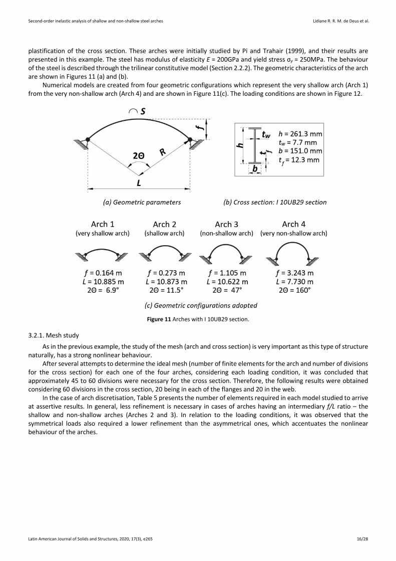
This section is intended to verify the influence of the loading conditions and the rise-to-span ratio f/L on arches with I 10UB29 section. It is an even more compact profile than the one presented in the previous example, with λ = 6.14 < λp = 10.75 (NBR 8800, 2008) and, therefore, local buckling is not considered since it does not occur before the



plastification of the cross section. These arches were initially studied by Pi and Trahair (1999), and their results are presented in this example. The steel has modulus of elasticity E = 200GPa and yield stress σy = 250MPa. The behaviour of the steel is described through the trilinear constitutive model (Section 2.2.2). The geometric characteristics of the arch are shown in Figures 11 (a) and (b).

Numerical models are created from four geometric configurations which represent the very shallow arch (Arch 1) from the very non-shallow arch (Arch 4) and are shown in Figure 11(c). The loading conditions are shown in Figure 12.

Figure 11 Arches with I 10UB29 section.

3.2.1. Mesh study

As in the previous example, the study of the mesh (arch and cross section) is very important as this type of structure naturally, has a strong nonlinear behaviour.

After several attempts to determine the ideal mesh (number of finite elements for the arch and number of divisions for the cross section) for each one of the four arches, considering each loading condition, it was concluded that approximately 45 to 60 divisions were necessary for the cross section. Therefore, the following results were obtained considering 60 divisions in the cross section, 20 being in each of the flanges and 20 in the web.

In the case of arch discretisation, Table 5 presents the number of elements required in each model studied to arrive at assertive results. In general, less refinement is necessary in cases of arches having an intermediary f/L ratio – the shallow and non-shallow arches (Arches 2 and 3). In relation to the loading conditions, it was observed that the symmetrical loads also required a lower refinement than the asymmetrical ones, which accentuates the nonlinear behaviour of the arches.



Figure 12 Adopted loading conditions.

3.2.2. Equilibrium path

In this section, the nonlinear equilibrium paths for the arches under loading conditions shown in Figure 12 are displayed through Figures 13–17: concentrated load applied at the top of the arch (Figure 13); concentrated load applied to 1/4 of the horizontal projection of the arch (Figure 14); vertical load distributed throughout the arch (Figure 15); partial vertical load distributed in half of the arch (Figure 16); and radial load (Figure 17). In the representation of the structure response, the vertical displacement, vc, at the top of the arch or vL/4 at the 1/4 of the arch span is considered a reference and dimensionless by the rise of the arch, f; the load, represented by Q or q, is parameterised through the second elastic buckling load of a column with equivalent length S (about its major axis, Pi and Trahair, 1999).

Table 5 Number of elements used in the discretisation of the arches.

Loading condition Arches

Arch 1 (2Θ = 6.9°)

Arch 2 (2Θ = 11.5°)

Arch 3 (2Θ = 47°)

Arch 4 (2Θ = 160°)

Radial load 16 8 8 36 Concentrated load (L/2) 16 8 8 60 Concentrated load (L/4) 60 36 60 200

Distributed load (EA) 8 36 16 60 Distributed load (HA) 200 100 100 200

Note: EA = load in the entire arch; HA = load in a half of the arch



Figure 13 Equilibrium path: arches under concentrated load at the top.

Figure 14 Equilibrium path: arches under concentrated load at L/4.



Figure 15 Equilibrium path: arches under vertical distributed load in entire arch.

Figure 16 Equilibrium path: arches under vertical distributed load in a half arch.



Figure 17 Equilibrium path: arches under radial load.

The results obtained via CS-ASA were compared to those of Pi and Trahair (1999) for the arches under concentrated load and radial load. The MASTAN2 software was used in the study of all the models and contributes with two different results, one adopting the tangent modulus of elasticity, Et, and the other adopting the modified tangent modulus of elasticity, Etm. The last one incorporates in its expression the influence of the bending moment (Gonçalves, 2013; Ziemian and McGuire, 2002).

As evident from these figures, the results found via CS-ASA are close to those of the literature and MAS-TAN2 in most cases. According to Pi and Trahair (1999), for concentrated loads and radial loads, the Arches 1 and 2 (very shallow and shallow, respectively) generally lose stability by snap-through. The Arches 3 and 4 (non-shallow and very non-shallow, respectively) usually lose stability by bifurcation.

3.2.3. Study of rise-to-span ratio and full yield curve

Keeping the arch length S = 10.89m constant and varying the value of the internal angle 2Θ from 5° to 220°, the equilibrium paths shown in Figures 18 and 19 were obtained for 12 arches with different f/L values.



Figure 18 Equilibrium path for different values of f/L.



Figure 19 Equilibrium path: symmetric x asymmetrical (5° < 2Θ < 220°).



Figure 18(a) shows the nonlinear paths for the arches subjected to a concentrated load at the top of the arch (symmetric case) and Figure 18(b) shows the results considering the load concentrated in L/4 (asymmetric case). The rise-to-span ratio f/L exerts a great influence on the behaviour of the arches as can be seen in these figures.

For both loading cases, as the f/L value increases, that is, as the arch becomes less non-shallow, the critical load becomes higher as already seen in the previous example. In the symmetric case (Fig. 18(a)), the resistance initially increases rapidly at each f/L increase then increases more slowly until it stabilises between 0.3501 < f/L < 0.5, and the sequence falls to values of f/L > 0.5. In the asymmetric case (Figure 18(b)), the resistance increases sharply for the first three f/L ratios of the arch and then the increase becomes more constant for each increase of f/L.

To verify more clearly how these two load cases affect the arch behaviour for different f/L ratios, Figure 19 was drawn. This figure shows the equilibrium paths of the structure with internal angle 2Θ ranging from 5° to 220°.

Note that for 2Θ = 5°, a higher limit load is reached for the asymmetric loading case; for 2Θ = 20° the situation reverses, i.e., the arch with symmetric loading case becomes stronger. This difference increases until 2Θ = 100°. From this point, this difference decreases until 2Θ = 180°. For 2Θ = 200° and 2Θ = 220°, the arch under asymmetric loading case has an upper limit load.

Therefore, for this study, in the asymmetric loading case, the very shallow (2Θ <20°) and the very non-shallow (2Θ> 200°) arches presented better structural performance. For values of 20 ≤ 2Θ ≤ 200°, the better structural performance corresponds to the arches with symmetrical loading case.

3.3. Shed-type frame with steel arch

A complete structural system formed by five shed frames with steel arches is shown in Figure 20(a). A typical standard frame of this system with the details from geometry, and dimensions of I-sections used in columns and arches are presented in Figure 20(b) and 20(c), respectively. The steel used is the Q345B. The purlins (load entry points) are located every meter and the loading condition is represented by nine loads concentrated in the arch spaced equally. Table 6 shows the properties of the Q345B steel.

Figure 20 Steel Structural systems with shed-type frames.



This section aims to discuss the realisation of the SOIA of this standard shed-type frame that has a steel arch as the primary structural element. The model adopted for the residual stresses follows the one described in EN 1993-1-2 (2005) (Section 2.2.2).

Figure 21 shows the equilibrium path and the evolution of the deformed shape of the frame whose arch has a rise-to-span ration f/L = 0.05 (shallow arch). The results obtained using CS-ASA using a mesh with 10 and 16 finite elements for the columns and the arch, respectively, are compared to those obtained through MASTAN2. There is similarity between the equilibrium points reached with these two programs as well as the values of the limit loads obtained: 53.2kN in the CS-ASA and 53.1kN in the MASTAN2.

Table 6 Steel properties.

Steel properties

Q345B Modulus of Elasticity (E) 220 GPa

Yield stress (fy) 360.3 MPa

Point A Point C

Point B

0 0.2 0.4 0.6 0.8 1

Displacement vc ( m )

0

20

40

60

80

Load

P (

kN )

CS-ASAMASTAN2

A

B

C

Figure 21 Equilibrium path and deformed shape evolution to the fixed shed-type frame with steel arch.

Figure 22 shows the internal forces diagrams (axial force and bending moment) for the equilibrium configurations in the sections A and B marked in the equilibrium path of the frame (Figure 21).

Figure 22 Internal forces diagrams for the steel shed-type frame (A and B sections can be seen in Figure 21).



Figure 23 provides the plastification index of the arch sections when the limit load is reached. The points located where plastic hinges occurs are marked in red and the percentage of plastification in some sections is shown inside the ellipses indicated in Figure. The first plastic hinges form at the arch-column connection, and in the sequence, the plastic hinge formation occurs at the top of the arch as shown in Figure 22. The sections located on the columns did not degrade because the stiffness of the column profile is much larger than the stiffness of the arch profile.

Figure 23 Plastification index of selected steel arch sections.

4 FINAL REMARKS

The numerical formulations adopted in this paper allowed, with good precision, the analysis of the second-order inelastic behaviour of arches ranging from very shallow to very non-shallow with different loading and boundary conditions. The coupling of the RPHM, which considers the gradual cross-section plastification, to the Stain Compatibility Method (SCM), which was used in the evaluation of the full yield curves and in obtaining generalised axial and flexural stiffness, contributed to the success of the arches’ SOIA. The results obtained through the CS-ASA (Silva, 2009) presented good agreement with those in the literature and with those of the MASTAN2 analyses (McGuire et al., 2014) using the modified tangent modulus of elasticity, Etm. However, some specific comments deserve attention as follows:

Influence of the structure discretisation and cross section divisions:

In all the models analysed, the structure response was sensitive to the discretisation adopted primarily in relation to the number of finite elements along the arch. In the comparison of arches with the same value of length S and different values of internal angle 2Θ, it was found that structures with the values of 2Θ very small (very shallow arches) or very large (very non-shallow arches) required a better discretisation of the section transversal in relation to the others with intermediary values of 2Θ. Similarly, arches under asymmetric loading condition also demanded mesh refinement as this loading accentuates their nonlinear behaviour. With respect to the number of divisions in the cross section, there was great variation among the examples used. In some cases, a minimal reduction of the number of elements used in each case implied numerical instabilities, preventing CS-ASA to map the post-critical equilibrium path of the structure. In the future, an in-depth study can be performed by varying the incremental-iterative strategy in order to trace the complete equilibrium path with the least number of cross section divisions as possible.

Influence of the loading conditions:

In the case of the vertical concentrated loads, the position of the load had significant influence on the resistance of the arches with different rise-to-span ratio f/L. Therefore, a thorough study involving the positioning of the load specific to each arch configuration is necessary in order to extract its best structural performance. It is a relevant analysis for the arches used as main structural elements in bridges and roofs, with specific points of positioning of the concentrated loads. In case of the vertical uniformly distributed loads applied, the arches studied in Sections 3.2 and 3.3 had more uniform distribution of internal forces. Under radial loading, pinned arches were analysed (Section 3.2) and only compression forces were observed.

Influence of the rise-to-span ratio (f/L):

The equilibrium paths obtained showed good agreement with the literature data or numerical analyses performed via MASTAN2. In most of the cases studied, the loss of stability occurred through snap-through, a condition in which dynamic jumps for other equilibrium configurations may occur from a small increase in load. However, in some cases of very shallow arches, there also occurred stability loss by bifurcation. The rise-to-span ratio f/L of the arch showed great



influence on the structure resistance. For an arch of the same length S, the greater the value of f/L, the more resistant the arch. In addition to this typical behaviour of the arches, the position of the load applied also influences the relation of f/L versus critical load as observed in Figure 18.

Acknowledgments

The authors are grateful for the financial support received by from Brazilian National Council for Scientific and Technological Development (CNPq), Coordinating Agency for Advanced Training of High-Level Personnel (CAPES), Minas Gerais State (FAPEMIG), Federal University of Ouro Preto/PROPP. Special thanks to PAPERTRUE for the editorial review of this text.

Author’s Contributions: Conceptualization, LRRM de Deus, JL Silva, IJM Lemes and RAM Silveira; Numerical Methodology, JL Silva and IJM Lemes; Numerical Investigation, LRRM de Deus, JL Silva and RAM Silveira; Writing - original draft, LRRM de Deus and JL Silva; Writing - review & editing, LRRM de Deus, JL Silva, IJM Lemes and RAM Silveira; Funding acquisition, RAM Silveira; Supervision, RAM Silveira.

Editor: Pablo Andrés Muñoz Rojas.

References

ADINA, 2005. ADINA R & D, Inc. / K.J. Bathe.

AISC, 2016. Specification for structural steel buildings. American Institute of Steel Construction, Chicago, Illinois, USA.

ANSYS, 2008. Product Launcher Release 11.0.

BATTINI, J. M., 2002. Co-rotational beam elements in instability problems. Ph.D Thesis. Royal Institute of Technology. Department of Mechanics, Stockholm, Sweden.

BRADFORD, M. A.; PI, Y.-L., 2015. Geometric Nonlinearity and Long-Term Behavior of Crown-Pinned CFST Arches. Journal of Structural Engineering, v. 141(8), p. 04014190/1–11.

BRADFORD, M. A.; PI, Y.-L.; YANG, G.; FAN, X.-C., 2015. Effects of approximations on nonlinear in-plane elastic buckling and postbuckling analyses of shallow parabolic arches. Engineering Structures, v. 101, p. 58–67.

BRADFORD, M. A.; UY, B.; PI, Y.-L., 2002. In-Plane Elastic Stability of Arches under a Central Concentrated Load. Journal of Engineering Mechanics, v. 128(7), p. 710–719.

CALDAS, R. B., 2004. Análise Numérica de Pilares Mistos Aço-Concreto. Dissertação de Mestrado. Programa de Pós-Graduação em Engenharia Civil, Universidade Federal de Ouro Preto, Ouro Preto, MG, Brasil.

CHAN, S. L., 1988. Geometric and material nonlinear analysis of beam-columns and frames using the minimum residual displacement method. International Journal for Numerical Methods in Engineering, v. 26, p. 2657–2669.

CHEN, S.; TENG, J. G.; CHAN, S. L., 2001. Design of biaxially loaded short composite columns of arbitrary section. Journal of Structural Engineering, v. 127(6), p. 678–685.

CHHANG, S.; BATTINI, J.-M.; HJIAJ, M., 2017. Energy-momentum method for co-rotational plane beams: A comparative study of shear exible formulations. Finite Elements in Analysis and Design, v. 134, p. 41–54.

CHIOREAN, C. G., 2013. A computer method for nonlinear inelastic analysis of 3D composite steel-concrete frame structures. Engineering Structures, v. 57, p. 125–152.

DIMOPOULOS, C. A.; GANTES, C. J., 2008. Design of circular steel arches with hollow circular cross-sections according to EC3. Journal of Constructional Steel Research, v. 64, p. 1077–1085.

ECCS, 1983. Ultimate limit state calculation of sway frames with rigid joints. European Convention for Constructional Steelwork, pub. n°. 33.



EN 1993-1-2 - European Committee for Standardization, 2005. Eurocode 3: Design of Steel Structures, Parte 1-2: General Rules, Structural Fire Design. Brussels.

GONÇALVES, G.A., 2013. Modelagem do comportamento inelástico de estruturas de aço: membros sob flexão em torno do eixo de menor inércia. Dissertação de Mestrado. Programa de Pós-Graduação em Engenharia Civil, Universidade Federal de Ouro Preto, Ouro Preto, MG, Brasil.

GUO, Y.-L.; ZHAO, S.-Y.; PI, Y.-L.; BRADFORD, M. A.; DOU, C., 2015. An experimental study on out-of-plane inelastic buckling strength of fixed steel arches. Engineering Structures, v. 98, p. 118–127.

GUO, Y.-L.; CHEN, H.; PI, Y.-L.; BRADFORD, M. A., 2016b. In-plane strength of steel arches with a sinusoidal corrugated web under a full-span uniform vertical load: Experimental and numerical investigations. Engineering Structures, v. 110, p. 105–115.

HAMED, E.; CHANG, Z.-T.; RABINOVITCH, O., 2015. Strengthening of Reinforced Concrete Arches with Externally Bonded Composite Materials: Testing and Analysis. Journal of Composites for Construction, v. 19(1), p. 04014031/1–15.

HEIDARPOUR, A.; PHAM, T. H.; BRADFORD, M. A., 2010a. Nonlinear thermoelastic analysis of composite steel–concrete arches including partial interaction and elevated temperature loading. Engineering Structures, v. 32(10), p. 3248–3257.

LEMES, Í. J. M.; SILVEIRA, R. A. M.; SILVA, A. R. D.; ROCHA, P. A. S., 2017. Nonlinear analysis of two-dimensional steel, reinforced concrete and composite steel-concrete structures via coupling SCM/RPHM. Engineering Structures, v. 147, p. 12–26.

LEMES, I. J. M., 2018. Estudo Numérico Avançado de Estruturas de Aço, Concreto e Mistas. Tese de Doutorado. Programa de Pós-Graduação em Engenharia Civil, Universidade Federal de Ouro Preto, Ouro Preto, MG, Brasil.

MCGUIRE, W.; GALLAGHER, R. H.; ZIEMIAN, R. D., 2014. Matrix structural analysis, 2nd Edition. Copyright by Ronald D. Ziemian.

MOON, J.; YOON, K.-Y.; LEE, T.-H.; LEE, H.-E., 2007. In-plane elastic buckling of pin-ended shallow parabolic arches. Engineering Structures, v. 29(10), p. 2611–2617.

NBR 8800, 2008. Projeto de estruturas de aço e de estruturas mistas de aço e concreto de edifícios. Associação Brasileira de Normas Técnicas.

NUNES, P. C. C., 2009. Teoria do arco de alvenaria: uma perspectiva histórica. Dissertação de Mestrado em Estruturas e Construção Civil. Departamento de Engenharia Civil e Ambiental, Universidade de Brasília, Brasília, DF, Brasil.

OLIVEIRA, G. C.; SILVA, W. T. M., 2017. Análise não-linear de arcos utilizando o elemento de viga unificado bernoulli-timoshenko e a formulação co-rotacional. REEC – Revista eletrônica de engenharia civil, v. 13(2), p. 1–16.

PI, Y.-L.; BRADFORD, M. A., 2004. In-plane strength and design of fixed steel I-section arches. Engineering Structures, v. 26(3), p. 291–301.

PI, Y.-L.; BRADFORD, M. A., 2012a. Non-linear in-plane analysis and buckling of pinned–fixed shallow arches subjected to a central concentrated load. International Journal of Non-Linear Mechanics, v. 47(4), p. 118–131.

PI, Y.-L.; BRADFORD, M. A., 2013a. Nonlinear elastic analysis and buckling of pinned–fixed arches. International Journal of Mechanical Sciences, v. 68, p. 212–223.

PI, Y.-L.; BRADFORD, M. A., 2014. Effects of nonlinearity and temperature field on in-plane behaviour and buckling of crown-pinned steel arches. Engineering Structures, v. 74, p. 1–12.

PI, Y.-L.; BRADFORD, M. A. 2015. In-Plane Analyses of Elastic Three-Pinned Steel Arches. Journal of Structural Engineering, v. 141(2), p. 06014009/1–4.

PI, Y.-L.; BRADFORD, M. A.; GUO, Y.-L., 2016. Revisiting Nonlinear In-Plane Elastic Buckling and Postbuckling Analysis of Shallow Circular Arches under a Central Concentrated Load. Journal of Engineering Mechanics, v. 142(8), p. 04016046/1–8.

PI, Y- L.; BRADFORD, M. A.; TIN-LOI, F., 2008b. In-plane strength of steel arches. Advanced Steel Construction, v. 4(4), p. 306–322.

PI, Y.-L.; BRADFORD, M. A.; UY, B., 2002. In-plane stability of arches. International Journal of Solids and Structures, v. 39(1), p. 105–125.

PI, Y.-L.; LIU, C.; BRADFORD, M. A.; ZHANG, S., 2012. In-plane strength of concrete-filled steel tubular circular arches. Journal of Constructional Steel Research, v. 69(1), p. 77–94.



PI, Y. L.; TRAHAIR, N. S., 1994a. Nonlinear Inelastic Analysis of Steel Beam-Columns. I: Theory. Journal of Structural Engineering, v. 120(7), p. 2041–2061.

PI, Y. L.; TRAHAIR, N. S., 1994b. Nonlinear Inelastic Analysis of Steel Beam-Columns. II: Applications. Journal of Structural Engineering, v. 120(7), p. 2062–2085.

PI, Y.-L.; TRAHAIR, N. S., 1996a. In-plane inelastic buckling and strengths of steel arches. Journal of Structural Engineering, v. 122, p. 734–747.

PI, Y.-L.; TRAHAIR, N. S., 1999. In-plane buckling and design of steel arches. Journal of Structural Engineering, v. 125, p. 1291–1298.

SFAKIANAKIS, M. G., 2002. Biaxial bending with axial force of reinforced, composite and repaired concrete section of arbitrary shape by fiber model and computer graphics. Advances in Engineering Software, v. 33, p. 227–242.

SILVA, A. R. D., 2009. Sistema computacional para análise avançada estática e dinâmica de estruturas metálicas. Tese de Doutorado. Programa de Pós-Graduação em Engenharia Civil, Universidade Federal de Ouro Preto, Ouro Preto, MG, Brasil.

SILVA, J. L., 2016. Formulações corrotacionais 2D para análise geometricamente não linear de estruturas reticuladas. Dissertação de Mestrado. Programa de Pós-Graduação em Engenharia Civil, Universidade Federal de Ouro Preto, Ouro Preto, MG, Brasil.

SPOORENBERG, R. C.; SNIJDER, H. H.; HOENDERKAMP, J. C. D., 2012a. A theoretical method for calculating the collapse load of steel circular arches. Engineering Structures, v. 38, p. 89–103.

SUSSEKIND, J.C., 1981. Curso de análise estrutural. Porto Alegre: Globo, v. 3, 6 edn.

TANG, Y. Q.; ZHOU, Z. H.; CHAN, S. L., 2015. Nonlinear beam-column element under consistente deformation. International Journal of Structural Stability and Dynamics, v. 15(5), p. 1450068/1–24.

TRAHAIR, N. S.; PI, Y.-L.; CLARKE, M. J.; PAPANGELIS, J. P., 1997. Plastic Design of Steel Arches. Advances in Structural Engineering, v. 1(1), p. 1–9.

TURNER, J., 1996. The dictionary of art. London: Macmillan.

XU, Y.J.; GUI, X.M.; ZHAO, B.; ZHOU, R.Q., 2014. In-Plane Elastic Stability of Arches under a Radial Concentrated Load. Engineering, v. 6, p. 572–583.

YANG, Y.; KUO, S., 1994. Theory & analysis of nonlinear framed structures. [S.l.]. New York: Prentice Hall.

ZIEMIAN, R. D.; MCGUIRE, W., 2002. Modified tangent modulus approach, a contribution to plastic hinge analysis. Journal of Structural Engineering, v. 128, p. 1301–1307.

ZHOU, Y.; CHANG, W.; STANCIULESCU, I., 2015. Nonlinear stability and remote unconnected equilibria of shallow arches with asymmetric geometric imperfections. International Journal of Non-Linear Mechanics.

ZUBYDAN, A. H., 2013. Inelastic large defletion analysis of space steel frames including H-shaped cross-section members. Engineering Structures, v. 48, p. 155–165.

Documents

a , Ricardo A. M. Silveiraa* , Ígor J. M. Lemesb , Jéssica