A REVIEW OF CRITERIA OF FIT FOR HYDROLOGICAL MODELS

International Research Journal of Engineering and Technology (IRJET) e-ISSN: 2395-0056

Volume: 04 Issue: 11 | Nov -2017 www.irjet.net p-ISSN: 2395-0072

© 2017, IRJET | Impact Factor value: 6.171 | ISO 9001:2008 Certified Journal | Page 1765

A REVIEW OF CRITERIA OF FIT FOR HYDROLOGICAL MODELS

M. Waseem1*, N. Mani2, G. Andiego3, M. Usman4

1PhD Scholar, Faculty of agriculture and environmental sciences, Universität Rostock, Germany

2Jounior Scientist, Sahasrara Earth services & Resources Ltd, Coimbatore, India 3Director, Water resources and environmental services department, Nairobi, Kenya

4PhD Scholar, Institute of water resources and water supply, TUHH Hamburg, Germany

---------------------------------------------------------------------***---------------------------------------------------------------------

Abstract - Hydrological model performance and its behavior is evaluated by comparison of observed and simulated variables. Mostly, the comparison is done between measured and simulated flows. Hydrologist use efficiency criteria to know the closeness of the observed and model- simulated values. Correlation-based methods have been used widely to evaluate the model performance. These measures are sensitive to peak flows but insensitive for low flow values, due to these limitations Nash-Sutcliffe efficiency (E) and coefficient of determination (R2) can give better agreement even for very poor models. So different modifications to these criteria are presented in this study. This paper also emphasizes on different efficiency criteria, their pros and cons, and suitable conditions for each of the different efficiency criteria. In this study goodness of fit has been tested for three different scenarios, and it is recommended that the use of correlation-based measures alone for model evaluation is not suitable, it should be a combination of different efficiency criteria. Key Words: Criteria of fit, correlation-based measures, NSE, R2

1. INTRODUCTION The river basin or catchment is a geographical scale generally used to manage the water resources. In a catchment, all the precipitation in the watershed will be added to the flow at a single outlet. At the outlet, water can be considered as a source of risk or damage in terms of flood, or can be considered as a source for satisfying the human needs in term of irrigation or drinking water. In both scenarios, it is essential to measure the water flowing into the stream in terms of its temporal distribution and volume (Krause, Boyle, and Base, 2005). Modelling involves empirical idealization and simplification of catchments. The operations of simplification and separation of precipitation introduce errors because of inadequate knowledge about the interactions of all the components within a watershed (Nash & Sutcliffe, 1970). Every hydrological model has some limitations, as it uses some simplification and empirical idealism, which results in an error between the observed and simulated discharge. So it is necessary to choose an appropriate model with a minimum error to simulate the rainfall-runoff relation near to the reality as much as possible (Krause, Boyle, and Base, 2005).

According to US EPA (2002), for acceptable results, models should be scientifically sound, robust and defensible. For such a model, it has to undergo the process of sensitivity analysis, model calibration, and validation. Sensitivity analysis is the determination of the response of the model output with respect to the input and in this process key model parameters are identified. In calibration, the identified parameters are determined by comparison of observed and predicted discharges. The last process of validation is a confirmation that the parameters and by extension the model produces sufficiently accurate predictions. However, a footnote should always be added about the uncertainties of the results (Moriasi et al, 2007). Because of the errors introduced by simplification of catchments during modeling, there usually are differences between the actual and simulated runoff. The evaluation of these differences forms the basis of model performance assessment. The purpose of the performance criteria is not only to find out the closeness of fit but also to use the findings to improve the models (Krause, Boyle, and Base, 2005). The model performance assessment is done either subjectively or objectively. In the subjective assessment, visual inspection of the closeness of fit between the actual and simulated discharges is done and the systematic (under-estimation/overestimation) or dynamic (periodic pattern) behavior of the model is noted. The objective assessment involves mathematical analysis of the closeness of fit of the two discharges and it is known as the efficiency criteria (Krause, Boyle, and Base, 2005). This means that the lower the error between observed and simulated runoff discharges, the higher the efficiency of the model and the more accurately it can be used to predict historical and future discharges. Most of the efficiency criteria are simply summations of the individual errors at each time step of a hydrograph which is then normalized by a measure of variability in the observations (Krause, Boyle, and Base, 2005). Most often the efficiency of a model is based solely on how well the predicted values fit the observed values, the assumption being that the observed data is error free while this is not necessarily always the case (Moriasi et al, 2007). There are numerous efficiency criteria, which have been put forward. According to Legates & McCabe (1999) and Moriasi et al. (2007), a good efficiency criterion should have at least three important components i.e. one dimensionless statistic,




one absolute error index statistic and one graphical technique. The objectives of this paper are i) Review a selection of efficiency criteria, show their

limits and recommend mitigation measures;

ii) Evaluate factors which affect model performance recommend mitigation measures;

Iii) Recommend guidelines on model evaluation for future reference.

Since in initial times of hydrological modeling, there was always a need to evaluate the model result and to know their flow prediction efficiency. Initial developments of conceptual models, Dawdy and O'Donnell (1965) and Linsley and Crawford (1960), measured the model residuals by plotting simulated and observed hydrographs or by knowing the difference in percentage between simulated and observed flows. Moreover, computation periods in early times were a major limitation and probably restricted the calculation of different evaluation criteria. While, the question of how to evaluate model performance, was often recognized as a vital issue. Nash and Sutcliffe (1970) propose an efficiency index for hydrological simulations evaluation. The aim was to offer an objective mean for giving a benchmark to a simulation. This proved to be a very worthy try as their index remains most extensively used in hydrological modeling regardless of its identified flaws (Gupta et al, 2009). Although after doing all these efforts, model evaluation remains a quite complex process and is related strongly to the modeling objectives.

2. METHODOLOGY 2.1 Study Area Data Basis To review the performance of the efficiency criteria, three papers Moriasi et al. (2007), Gupta et al. (2009) and Krause et al. (2005) have been used with different study area and data. The paper by Moriasi et al. (2007), was based on a previous modeling study by Arnold et al. (1998), where the SWAT2005 modeling tool was applied to the Leon River basin in Texas, USA. Average monthly observed discharged values were compared against simulated values. The paper by (Krause, Boyle, and Base, 2005) used daily discharge data from Wilde Gera catchment in Germany over the period November 1990 to April 1991. A proper model was not used to simulate the data but synthetic data was generated to act as simulated discharge emphasizing different types of errors (Krause and Flugel 2005). The paper by Gupta et al. (2009) used data from 49 Australian Basins between a period of September 1990 to August 2000. The daily data was used by a rainfall-runoff model to predict discharges from the basin.

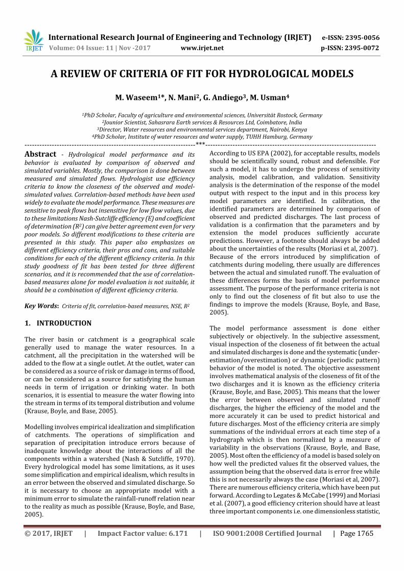
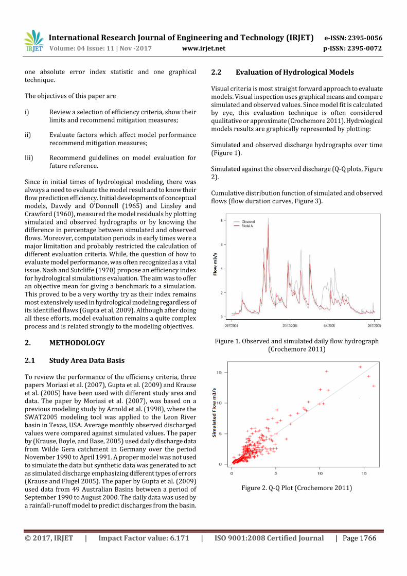
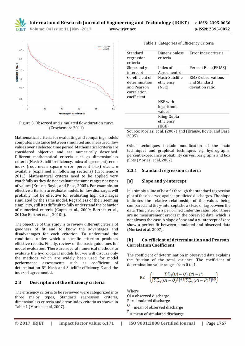
2.2 Evaluation of Hydrological Models Visual criteria is most straight forward approach to evaluate models. Visual inspection uses graphical means and compare simulated and observed values. Since model fit is calculated by eye, this evaluation technique is often considered qualitative or approximate (Crochemore 2011). Hydrological models results are graphically represented by plotting: Simulated and observed discharge hydrographs over time (Figure 1). Simulated against the observed discharge (Q-Q plots, Figure 2). Cumulative distribution function of simulated and observed flows (flow duration curves, Figure 3).

Figure 1. Observed and simulated daily flow hydrograph (Crochemore 2011)

Figure 2. Q-Q Plot (Crochemore 2011)




Figure 3. Observed and simulated flow duration curve (Crochemore 2011)

Mathematical criteria for evaluating and comparing models computes a distance between simulated and measured flow values over a selected time period. Mathematical criteria are considered objective and are numerically described. Different mathematical criteria such as dimensionless criteria (Nash-Sutcliffe efficiency, index of agreement), error index (root mean square error, percent bias) etc., are available (explained in following sections) (Crochemore 2011). Mathematical criteria need to be applied very watchfully as they do not evaluate the same ranges nor types of values (Krause, Boyle, and Base, 2005). For example, an effective criterion to evaluate models for low discharges will probably not be effective for evaluating high discharges simulated by the same model. Regardless of their seeming simplicity, still it is difficult to fully understand the behavior of numerical criteria (Gupta et al., 2009; Berthet et al., 2010a; Berthet et al., 2010b). The objective of this study is to review different criteria of goodness of fit and to know the advantages and disadvantages for each criterion. To understand the conditions under which a specific criterion produces effective results. Finally, review of the basic guidelines for model evaluation. There are several numerical methods to evaluate the hydrological models but we will discuss only the methods which are widely been used for model performance assessments such as coefficient of determination R2, Nash and Sutcliffe efficiency E and the index of agreement d.

2.3 Description of the efficiency criteria The efficiency criteria to be reviewed were categorized into three major types, Standard regression criteria, dimensionless criteria and error index criteria as shown in Table 1 (Moriasi et al, 2007).

Table 1: Categories of Efficiency Criteria Standard regression criteria

Dimensionless criteria

Error index criteria

Slope and y-intercept

Index of Agreement, d

Percent Bias (PBIAS)

Co-efficient of determination and Pearson correlation coefficient

Nash-Sutcliffe efficiency (NSE);

RMSE-observations and Standard deviation ratio

NSE with logarithmic values

Kling-Gupta efficiency (KGE)

Source: Moriasi et al. (2007) and (Krause, Boyle, and Base, 2005). Other techniques include modification of the main techniques and graphical techniques e.g. hydrographs, percent exceedance probability curves, bar graphs and box plots (Moriasi et al, 2007).

2.3.1 Standard regression criteria [a] Slope and y-intercept It is simply a line of best fit through the standard regression plot of the observed against predicted discharges. The slope indicates the relative relationship of the values being compared and the y-intercept shows lead or lag between the data. This criterion is performed under the assumption there are no measurement errors in the observed data, which is not always the case. A slope of one and a y-intercept of zero show a perfect fit between simulated and observed data (Moriasi et al, 2007).

[b] Co-efficient of determination and Pearson Correlation Coefficient The coefficient of determination in observed data explains the fraction of the total variance. The coefficient of determination value ranges from 0 to 1.

Where Oi = observed discharge Pi = simulated discharge

= mean of observed discharge

= mean of simulated discharge




The coefficient of Determination having a value of one indicates better agreement, while the value of zero reflect that there is no co-relation (predicted and observed values are equal) (Legates and McCabe, 1999). The coefficient of Determination has some limitations as it evaluates only the linear relationship between variables. It can be explained as if Pi = (AOi + B), where A = non zero value, B = any value. In this case coefficient of determination (R2) will be equal to one, this reflects that R2 is very exhaustive to additive and proportional differences between observed and model simulated values (Willmott, 1981). Hence higher values of coefficient of determination can be achieved even when observed and model simulated values vary significantly. The model would present a serious error in these situations. Moreover, co-relation based measures are sensitive to outliers instead of values which are near to the mean. Coefficient of determination (R2) value will greatly be affected by a single outlier, which will result in bias in model evaluation (Legates and McCabe, 1999). Adjustment factor was introduced to overcome the limitations in co-relation based methods (McCuen and Snyder, 1975).

Where Oi = observed discharge Pi = simulated discharge

= mean of observed discharge

= mean of simulated discharge Observed and predicted co-relation value is multiplied by an adjustment factor to account for the differences between predicted and observed standard deviations. But adjustment factor also has some limitations. In case of higher values of model predicted variance, use of adjustment factor will result in higher values of co-relation and can be more than one in extreme cases. So the use of adjustment factor is not always recommended (McCuen and Snyder, 1975).

2.3.2 Dimensionless Criteria [a] Index of Agreement, d It was introduced to overcome the insensitivities of NSE and coefficient of determination and is simply the ratio of the mean square error and the potential error. Its values range between 0 and 1, with 1 denoting a perfect fit while zero means no fit at all (Krause, Boyle, and Base, 2005). The index of agreement can detect proportional and additive differences in the observed and simulated means (Moriasi et al, 2007). It’s determined as follows;

Where; Oi – Observed discharge; Pi – Predicted discharge; Õ – Mean of observed discharge; As is apparent in the formula, the criterion is still insensitive to low flows and it also returns high efficiency values even in poorly performing models and this results in a narrow range for calibration (Krause, Boyle, and Base, 2005).

[b] Nash-Sutcliffe Efficiency (NSE) It is one of the most widely used despite its widely-reported inadequacies. It is basically the absolute difference between observed and predicted which is then normalized by the variance of the observed discharge to get rid of any bias. The range lies between 1 and -∞, with 1 being the perfect fit (Krause, Boyle, and Base, 2005).

Where; Oi – Observed discharge Pi – Predicted discharge Õ – Mean of observed discharge The numerator shows that smaller errors will become smaller while larger errors will become larger. This is the major disadvantage of the NSE criterion as it leads to overestimation or underestimation depending on the dominant error of the model under examination. Another disadvantage is that it uses the observed mean in calculating the variance for normalization (Numerator). This means that for catchments with highly variable discharges, it leads to overestimation of the efficiency. It is therefore advised that the observed seasonal mean be used instead (Krause, Boyle, and Base, 2005).

2.3.3 Error Index Criteria [a] Percent Bias (PBIAS) It measures the average negative deviation of the predicted data from the observed data with an optimum value of 0% meaning no deviation. It is calculated as follows (Moriasi et al, 2007).




Where; Oi – Observed discharge; Pi – Predicted discharge; RMSE-observations and Standard deviation ratio This criterion normalizes the RMSE with the standard deviation of the observed values. It is calculated as follows; (Moriasi et al, 2007)

Where; Oi – Observed discharge; Pi – Predicted discharge; Õ – Mean of observed discharge;

2.3.4 Modified Criteria [a] Modified forms of d and NSE To increase the sensitivity of both criteria, apart from using the logarithmic values of observed and predicted flows, further modifications can be done as follows

Where;

J

Oi – Observed discharge; Pi – Predicted discharge; Õ – Mean of observed discharge; This would reduce the insensitivity to low discharges especially if j=1. It is also open to manipulation depending on the objective. For example, if the interest is flooded discharges, j can be higher values (Krause, Boyle, and Base, 2005).

[b] Kling-Gupta Efficiency (KGE) It is formulated by decomposition of the NSE into the various components and correcting the bias factors. It is calculated as follows; (Gupta et al, 2009)

And

Where;

Where; ED – Euclidian distance from the ideal point; EDs – Euclidian distance from the ideal point in the scaled space;

α = , a measure of relative variability of the predicted

and observed runoff σs and σo – Standard deviation of predicted and observed runoff r – Linear correlation coefficient between simulated and observed data

ß – Bias factor; where µ is the mean of observed

and simulated flows s – Scaling factors for the components.

3 RESULTS AND ANALYSIS 3.1 Model Calibration, Validation and

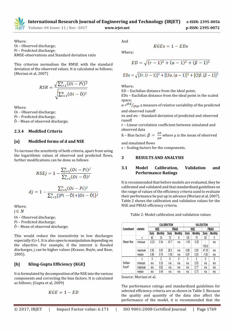
Performance Ratings It is recommended that before models are evaluated, they be calibrated and validated and that standardized guidelines on the range of values of the efficiency criteria used to evaluate their performance be put up in advance (Moriasi et al, 2007). Table 2 shows the calibration and validation values for the NSE and PBIAS efficiency criteria.

Table 2: Model calibration and validation values

Source: Moriasi et al. The performance ratings and standardized guidelines for selected efficiency criteria are as shown in Table 3. Because the quality and quantity of the data also affect the performance of the model, it is recommended that the




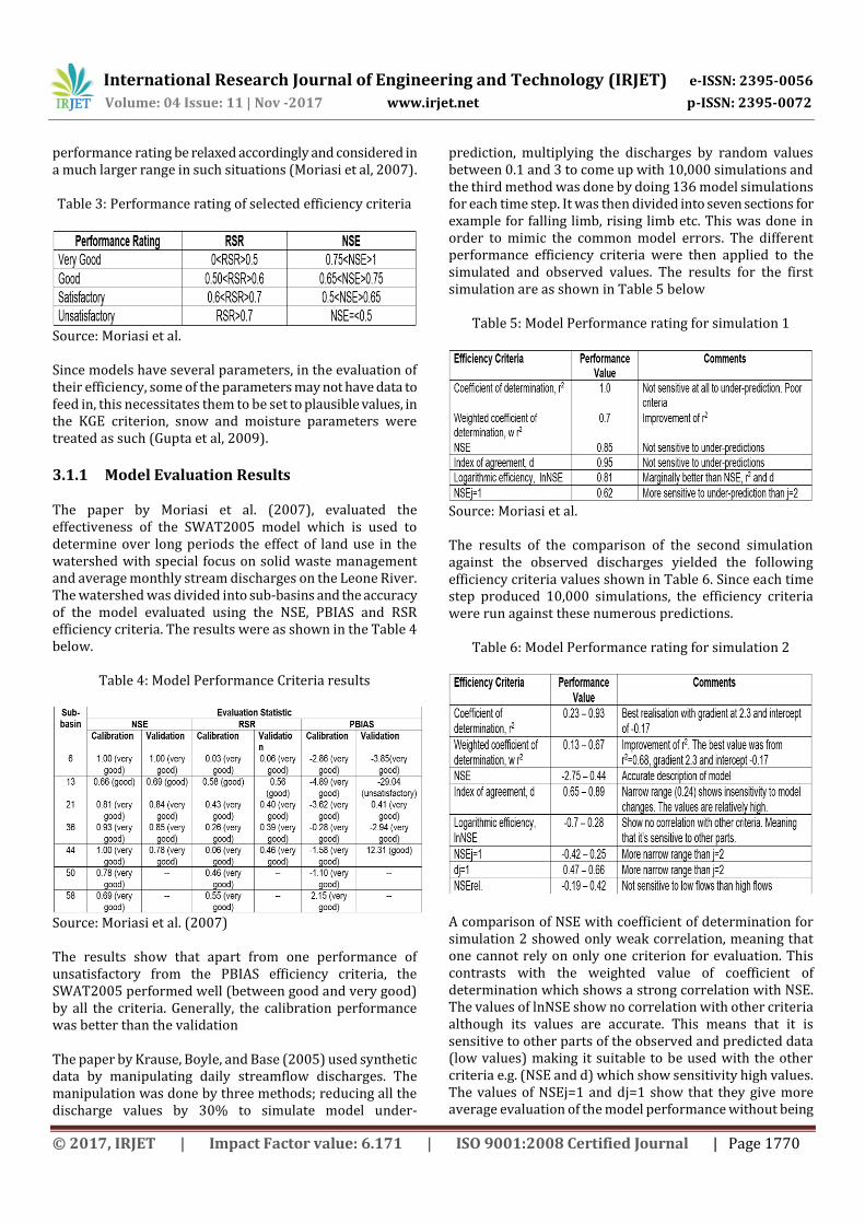
performance rating be relaxed accordingly and considered in a much larger range in such situations (Moriasi et al, 2007). Table 3: Performance rating of selected efficiency criteria

Source: Moriasi et al. Since models have several parameters, in the evaluation of their efficiency, some of the parameters may not have data to feed in, this necessitates them to be set to plausible values, in the KGE criterion, snow and moisture parameters were treated as such (Gupta et al, 2009).

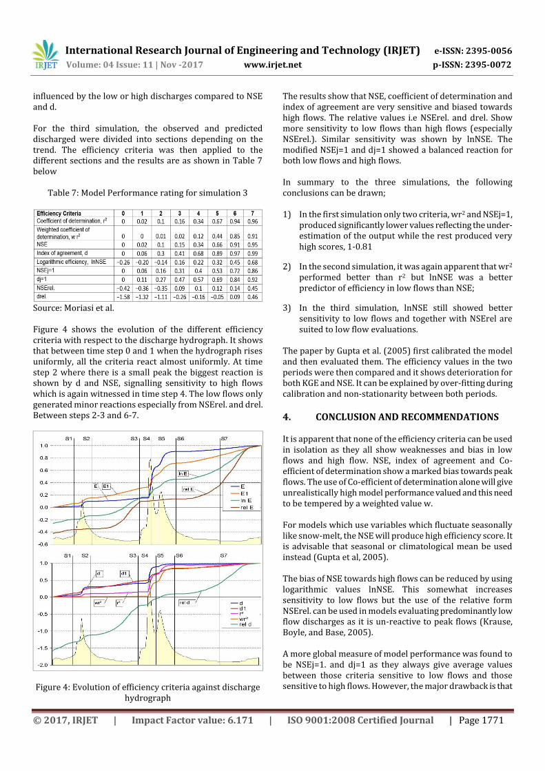
3.1.1 Model Evaluation Results The paper by Moriasi et al. (2007), evaluated the effectiveness of the SWAT2005 model which is used to determine over long periods the effect of land use in the watershed with special focus on solid waste management and average monthly stream discharges on the Leone River. The watershed was divided into sub-basins and the accuracy of the model evaluated using the NSE, PBIAS and RSR efficiency criteria. The results were as shown in the Table 4 below.

Table 4: Model Performance Criteria results

Source: Moriasi et al. (2007) The results show that apart from one performance of unsatisfactory from the PBIAS efficiency criteria, the SWAT2005 performed well (between good and very good) by all the criteria. Generally, the calibration performance was better than the validation The paper by Krause, Boyle, and Base (2005) used synthetic data by manipulating daily streamflow discharges. The manipulation was done by three methods; reducing all the discharge values by 30% to simulate model under-

prediction, multiplying the discharges by random values between 0.1 and 3 to come up with 10,000 simulations and the third method was done by doing 136 model simulations for each time step. It was then divided into seven sections for example for falling limb, rising limb etc. This was done in order to mimic the common model errors. The different performance efficiency criteria were then applied to the simulated and observed values. The results for the first simulation are as shown in Table 5 below

Table 5: Model Performance rating for simulation 1

Source: Moriasi et al. The results of the comparison of the second simulation against the observed discharges yielded the following efficiency criteria values shown in Table 6. Since each time step produced 10,000 simulations, the efficiency criteria were run against these numerous predictions.


A comparison of NSE with coefficient of determination for simulation 2 showed only weak correlation, meaning that one cannot rely on only one criterion for evaluation. This contrasts with the weighted value of coefficient of determination which shows a strong correlation with NSE. The values of lnNSE show no correlation with other criteria although its values are accurate. This means that it is sensitive to other parts of the observed and predicted data (low values) making it suitable to be used with the other criteria e.g. (NSE and d) which show sensitivity high values. The values of NSEj=1 and dj=1 show that they give more average evaluation of the model performance without being




influenced by the low or high discharges compared to NSE and d. For the third simulation, the observed and predicted discharged were divided into sections depending on the trend. The efficiency criteria was then applied to the different sections and the results are as shown in Table 7 below


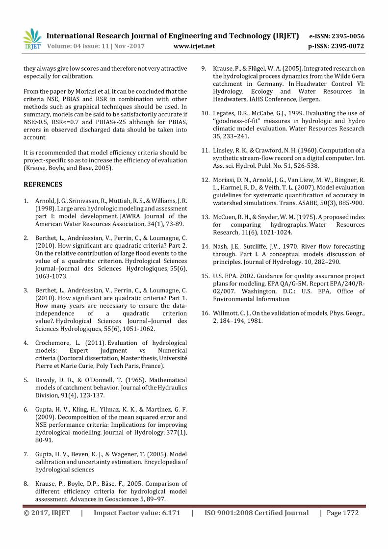
Source: Moriasi et al. Figure 4 shows the evolution of the different efficiency criteria with respect to the discharge hydrograph. It shows that between time step 0 and 1 when the hydrograph rises uniformly, all the criteria react almost uniformly. At time step 2 where there is a small peak the biggest reaction is shown by d and NSE, signalling sensitivity to high flows which is again witnessed in time step 4. The low flows only generated minor reactions especially from NSErel. and drel. Between steps 2-3 and 6-7.

Figure 4: Evolution of efficiency criteria against discharge hydrograph

The results show that NSE, coefficient of determination and index of agreement are very sensitive and biased towards high flows. The relative values i.e NSErel. and drel. Show more sensitivity to low flows than high flows (especially NSErel.). Similar sensitivity was shown by lnNSE. The modified NSEj=1 and dj=1 showed a balanced reaction for both low flows and high flows. In summary to the three simulations, the following conclusions can be drawn; 1) In the first simulation only two criteria, wr2 and NSEj=1,

produced significantly lower values reflecting the under-estimation of the output while the rest produced very high scores, 1-0.81

2) In the second simulation, it was again apparent that wr2

performed better than r2 but lnNSE was a better predictor of efficiency in low flows than NSE;

3) In the third simulation, lnNSE still showed better sensitivity to low flows and together with NSErel are suited to low flow evaluations.

The paper by Gupta et al. (2005) first calibrated the model and then evaluated them. The efficiency values in the two periods were then compared and it shows deterioration for both KGE and NSE. It can be explained by over-fitting during calibration and non-stationarity between both periods.

4. CONCLUSION AND RECOMMENDATIONS It is apparent that none of the efficiency criteria can be used in isolation as they all show weaknesses and bias in low flows and high flow. NSE, index of agreement and Co-efficient of determination show a marked bias towards peak flows. The use of Co-efficient of determination alone will give unrealistically high model performance valued and this need to be tempered by a weighted value w. For models which use variables which fluctuate seasonally like snow-melt, the NSE will produce high efficiency score. It is advisable that seasonal or climatological mean be used instead (Gupta et al, 2005). The bias of NSE towards high flows can be reduced by using logarithmic values lnNSE. This somewhat increases sensitivity to low flows but the use of the relative form NSErel. can be used in models evaluating predominantly low flow discharges as it is un-reactive to peak flows (Krause, Boyle, and Base, 2005). A more global measure of model performance was found to be NSEj=1. and dj=1 as they always give average values between those criteria sensitive to low flows and those sensitive to high flows. However, the major drawback is that




they always give low scores and therefore not very attractive especially for calibration. From the paper by Moriasi et al, it can be concluded that the criteria NSE, PBIAS and RSR in combination with other methods such as graphical techniques should be used. In summary, models can be said to be satisfactorily accurate if NSE>0.5, RSR<=0.7 and PBIAS+-25 although for PBIAS, errors in observed discharged data should be taken into account. It is recommended that model efficiency criteria should be project-specific so as to increase the efficiency of evaluation (Krause, Boyle, and Base, 2005).

REFRENCES 1. Arnold, J. G., Srinivasan, R., Muttiah, R. S., & Williams, J. R.

(1998). Large area hydrologic modeling and assessment part I: model development. JAWRA Journal of the American Water Resources Association, 34(1), 73-89.

2. Berthet, L., Andréassian, V., Perrin, C., & Loumagne, C. (2010). How significant are quadratic criteria? Part 2. On the relative contribution of large flood events to the value of a quadratic criterion. Hydrological Sciences Journal–Journal des Sciences Hydrologiques, 55(6), 1063-1073.

3. Berthet, L., Andréassian, V., Perrin, C., & Loumagne, C. (2010). How significant are quadratic criteria? Part 1. How many years are necessary to ensure the data-independence of a quadratic criterion value?. Hydrological Sciences Journal–Journal des Sciences Hydrologiques, 55(6), 1051-1062.

4. Crochemore, L. (2011). Evaluation of hydrological models: Expert judgment vs Numerical criteria (Doctoral dissertation, Master thesis, Université Pierre et Marie Curie, Poly Tech Paris, France).

5. Dawdy, D. R., & O'Donnell, T. (1965). Mathematical models of catchment behavior. Journal of the Hydraulics Division, 91(4), 123-137.

6. Gupta, H. V., Kling, H., Yilmaz, K. K., & Martinez, G. F. (2009). Decomposition of the mean squared error and NSE performance criteria: Implications for improving hydrological modelling. Journal of Hydrology, 377(1), 80-91.

7. Gupta, H. V., Beven, K. J., & Wagener, T. (2005). Model calibration and uncertainty estimation. Encyclopedia of hydrological sciences

8. Krause, P., Boyle, D.P., Bäse, F., 2005. Comparison of different efficiency criteria for hydrological model assessment. Advances in Geosciences 5, 89–97.

9. Krause, P., & Flügel, W. A. (2005). Integrated research on the hydrological process dynamics from the Wilde Gera catchment in Germany. In Headwater Control VI: Hydrology, Ecology and Water Resources in Headwaters, IAHS Conference, Bergen.

10. Legates, D.R., McCabe, G.J., 1999. Evaluating the use of ‘‘goodness-of-fit” measures in hydrologic and hydro climatic model evaluation. Water Resources Research 35, 233–241.

11. Linsley, R. K., & Crawford, N. H. (1960). Computation of a synthetic stream-flow record on a digital computer. Int. Ass. sci. Hydrol. Publ. No. 51, 526-538.

12. Moriasi, D. N., Arnold, J. G., Van Liew, M. W., Bingner, R. L., Harmel, R. D., & Veith, T. L. (2007). Model evaluation guidelines for systematic quantification of accuracy in watershed simulations. Trans. ASABE, 50(3), 885-900.

13. McCuen, R. H., & Snyder, W. M. (1975). A proposed index for comparing hydrographs. Water Resources Research, 11(6), 1021-1024.

14. Nash, J.E., Sutcliffe, J.V., 1970. River flow forecasting through. Part I. A conceptual models discussion of principles. Journal of Hydrology. 10, 282–290.

15. U.S. EPA. 2002. Guidance for quality assurance project plans for modeling. EPA QA/G-5M. Report EPA/240/R-02/007. Washington, D.C.: U.S. EPA, Office of Environmental Information

16. Willmott, C. J., On the validation of models, Phys. Geogr., 2, 184–194, 1981.

Documents

A REVIEW OF CRITERIA OF FIT FOR HYDROLOGICAL MODELS