Int. J. Heavy Vehicle Systems, Vol. x, No. x, xxxx 1

Copyright © 200x Inderscience Enterprises Ltd.

A response spectral decomposition approach for the control of nonlinear mechanical systems

Corina Sandu* Associate Professor, Mechanical Engineering Department, Center for Vehicle Systems and Safety, Virginia Polytechnic Institute and State University, 104 Randolph Hall, Blacksburg, VA 24061 Fax: (540) 231-9100

Director, Advanced Vehicle Dynamics Laboratory, Center for Vehicle Systems and Safety, Virginia Polytechnic Institute and State University, 3103 Commerce Street, Blacksburg, VA 24061 Fax: (540) 231-0730 E-mail: csandu@vt.edu *Corresponding author

Adrian Sandu Associate Professor, Computer Science Department, Center for Vehicle Systems and Safety, Virginia Polytechnic Institute and State University, 2224 Knowledgeworks 2, 2200 Kraft Dr., Blacksburg, VA 24061 Fax: (540) 231-9218 E-mail: sandu@cs.vt.edu

Brendan J. Chan Mechanical Engineering Department, Advanced Vehicle Dynamics Laboratory, Center for Vehicle Systems and Safety, Virginia Polytechnic Institute and State University, 9A Randolph Hall, Blacksburg, VA 24061 Fax: (540) 231-9100 E-mail: bjchan@vt.edu

Mehdi Ahmadian Professor, Mechanical Engineering Department, Virginia Polytechnic Institute and State University, 123 Randolph Hall, Blacksburg, VA 24061 Fax: (540) 231-9100

Director, Center for Vehicle Systems and Safety, Director, Railway Technology Laboratory, 3103 Commerce Street, Blacksburg, VA 24061 Fax: (540) 231-0730 E-mail: ahmadian@vt.edu

Author: Please clarify which affiliation has to be included for first and last author.

2 C. Sandu et al.

Abstract: This study investigates a control methodology for dynamic systems based on representing all possible system responses under all possible values of the control variables. The underlying idea is to extend the system along the ‘control dimension’ and explicitly account for the dependence of the system state on control variables. A spectral discretisation along the ‘control dimension’ is employed. The optimal control values are chosen to obtain the desired parameterised system response. This approach has the advantage of allowing an inexpensive search for the optimal control values at each time increment without having to run the full nonlinear dynamic model. Numerical studies for the control of linear and nonlinear quarter-car models riding on various terrain profiles show promising results.

Keywords: control of mechanical systems; orthogonal polynomials; spectral decomposition.

Reference to this paper should be made as follows: Sandu, C., Sandu, A., Chan, B.J. and Ahmadian, M. (xxxx) ‘A response spectral decomposition approach for the control of nonlinear mechanical systems’, Int. J. Heavy Vehicle Systems, Vol. x, No. x, pp.xxx–xxx.

Biographical notes: Corina Sandu is an Assistant Professor of Mechanical Engineering at Virginia Tech. She received her Engineering Diploma in 1991 from the Bucharest Polytechnic Institute, her MS in 1995 and her PhD in 2000 in Mechanical Engineering from The University of Iowa. She worked at Michigan Tech as a Visiting and Research Faculty for three years. Since Sept. 2004 she has been the Director of the Advanced Vehicle Dynamics Laboratory. Her research concerns modelling and simulation of multibody dynamics under uncertainty, soil and terrain modelling, vehicle dynamics, tire and track modelling, and terramechanics. She received the Professional Engineers Publishing Award in 2003, and the SAE Ralph R. Teeor Educational Award in 2007. She is an active member of ASME, SAE, and ISTVS, a member of ASEE, a member on the editorial board of the International Journal of Vehicle Systems Modelling and Testing, and an associate editor of the Journal of Terramechanics. She authored and co-authored 12 journal papers, 32 peer-reviewed conference technical publications, more than 45 other conference papers, reports and presentations.

Adrian Sandu is an Associate Professor of Computer Science at Virginia Tech. His research interests are numerical methods and high performance computing. He has received his Diploma in Electrical Engineering in 1990 from the Bucharest Polytechnic Institute and both his MS in Computer Science and his PhD in Applied Mathematical and Computational Sciences in 1997 from the University of Iowa. He had a Howard Hughes post-doc at the Courant Institute at New York University. Between 1998 and 2003 he was an Assistant Professor in the Computer Science Department at Michigan Tech. He is the recipient of the NSF CAREER award in 2001, and the Professional Engineers Publishing Award in 2003. He is an active member of SIAM, and a member of ASME, ISTVS and SAE. He has authored and co-authored over 40 journal articles and numerous conference publications.

Brendan J. Chan is currently a PhD candidate affiliated with the Advanced Vehicle Dynamics Laboratory (part of the Center for Vehicle Systems and Safety) at Virginia Tech under the supervision of Dr. Corina Sandu. He received his Bachelor of Science Degree in Electrical Engineering in 2003 from Michigan Tech., specialising in electronic applications and control systems, and continued to pursue his graduate Degree in Mechanical Engineering at Virginia Tech His main area of research is modelling

Author: Please reduce career history of no more than 100 words for all author.

A response spectral decomposition approach 3

tire-ground vehicle interaction and vehicle dynamics. His supplementary area of research includes development of control algorithms for vehicle subsystems and multibody dynamics modelling. He is an active member of ASME and SAE. He received the Virginia Tech Graduate School Graduate Research and Development Project Grant in 2006 and the 2007 Virginia Tech Citizen Scholar Award for serving as the Chair of the College of Engineering Graduate Student Committee. He has co-authored three journal papers (one published two under review) and ten refereed conference publications.

Mehdi Ahmadian is a Professor of Mechanical Engineering at Virginia Tech, where he also holds the position of Director of Center for Vehicle Systems and Safety (CVeSS), and the Railway Technologies Laboratory (RTL). He is the founding director of CVeSS, RTL, Virginia Institute for Performance Engineering and Research (VIPER), and the Advanced Vehicle Dynamics Laboratory (AVDL). Dr. Ahmadian has authored more than 200 technical publications, and has made more than 100 technical presentations in topics related to advanced technologies for ground vehicles. He holds seven US and international patents, and has edited three technical volumes. He is currently Associate Editor of AIAA Journal and the journal of Shock Vibration, and has served as Associate Editor for ASME Journal of Vibration and Acoustics (1989–1996). He is a Fellow of American Society of Mechanical Engineers (ASME), a Senior Member of the American Institute for Aeronautics and Astronautics (AIAA), and a member of the Society for Automotive Engineers (SAE).

1 Introduction

In this paper we develop a method for the control of nonlinear systems based on representing all possible system responses under all possible values of the control variables. We are interested in mechanical systems, specifically in automotive applications. However, the approach is general and can be applied to any dynamical system.

The proposed approach constructs a response surface-like surrogate model of the dynamic system that maps the entire space of possible control variable values to the entire space of possible system responses. The synthesis of the control variable is then carried out using the surrogate model rather than the original full dynamic model. This approach has the advantage of allowing an inexpensive search for the optimal control values at each time increment. The method is computationally attractive when the dynamic system is highly nonlinear and expensive to simulate and when the number of control variables is relatively small. For this kind of systems the surrogate model can be easily constructed to approximate well the system behaviour and is very inexpensive to run.

The dynamical system is extended along the ‘control dimension’. This allows to explicitly accounting for the dependence of the system state on control variables. Specifically, the state is represented by its spectral decomposition along the control dimension. Numerically, the system response is parameterised by the set of spectral coefficients. The control problem is formulated as an optimisation problem with the cost function depending on the system state. The response parameterisation allows to easily formulating the explicit dependence of the cost function on the controls. The values of

4 C. Sandu et al.

the control variables are then chosen to obtain the desired system response using a polynomial function minimisation.

This paper is organised as follows. A short background on the formulations of the dynamics of mechanical systems is given. Next, we present our control approach, including the computational formulation and basis functions used in this study. The computational formulation is motivated by the applications of parameterised response to uncertainty quantification (Ghanem and Spanos, 1991a, 1991b; Xiu and Karniadakis, 2002). The optimisation procedure is described next. Several numerical results are included to illustrate the performance of the proposed control methodology. The new approach is compared with traditional methods (PI, PID and skyhook control). In the end, a summary of conclusions drawn from this study is given. We also included an appendix with orthogonal polynomial basis functions.

2 Background

The dynamics of a mechanical system is described by a system of second order Ordinary Differential Equations (ODE). If the system is constrained, then the formulation becomes a system of Differential Algebraic Equations (DAE). In this paper we consider the dynamics of the mechanical system described by a set of simultaneous fist order ODEs (Dorf and Bishop, 2001):

0 0 0, ( , , ; ), ( ) , .= = = ≤ ≤ Fy v v F t y v y t y t t tξ (1)

Here y ∈ ℜd are the generalised positions, , ∈ℜdv v the generalised velocities and accelerations respectively, and ξ ∈ Ω ⊂ ℜn the control variables. The dot notation represents differentiation with respect to time. The set Ω is the domain of all admissible values of the control variables.

The control problem on t ∈ [0, T] is formulated as an n-dimensional optimisation problem, where one minimises the value of a cost function at the final time T,

find that minimizes ( ( , ), ( , ), )J y T v Tξ ξ ξ ξ∈ Ω (2)

or a cost function defined by a time integral over the time horizon of interest,

0find that minimizes ( ( , ), ( , ), )d .

TJ y t v t tξ ξ ξ ξ∈Ω ∫ (3)

In Section 3.4 we will discuss the case of time dependent control variables ξ(t).

3 The control approach

The proposed approach is to extend the multi-body dynamic model along the parameterised control dimension. This allows a representation of the state of the system which explicitly accounts for the effect of controls. More exactly, the additional dimension allows characterising all possible system responses to all possible values of the control variables. The controls that lead to an optimal system response are then selected.

A response spectral decomposition approach 5

3.1 Spectral representation of the system response

At any moment in time, the state of the system equation (1) is a finite energy function of the control variables ξ = (ξ1 ≡ ξn) ∈ Ω, i.e.,

2 2( ) ( ), ( ) ( ), 1 .k ky t L v t L k d∈ Ω ∈ Ω ≤ ≤ (4)

Indeed, assuming that the domain Ω of all admissible controls is bounded, and that the position and velocity take finite values at each time moment we have:

2 2(| ( , ) | | ( , ) | )d .y t v tξ ξ ξΩ

+ < ∞∫ (5)

We construct a finite-dimensional approximation of the system response (as a function of the controls) by projecting it onto finite dimensional subspaces of L2(Ω). The subspaces are defined in terms of orthogonal polynomial basis functions. The resulting spectral approximation allows high order representations of the system response,

1 1

( ) ( ) ( ), ( ) ( ) ( ), 1 .S S

j j j jk k k k

j j

y t y t v t v t k dφ ξ φ ξ= =

= = ≤ ≤∑ ∑ (6)

We use subscripts to denote the components along the system dimension (i.e., position or velocity indices), and superscripts to denote components along the controls dimension (i.e., the spectral coefficients). The superscript-only notation will be used to represent the vector of spectral coefficients,

1

for all 1 .

j

j

jd

yy j S

y

= ≤ ≤

(7)

Formally, the control variables can be written using a similar polynomial expansion:

1

( ), 1 .S

j jk k

j

k nξ ξ φ ξ=

= ≤ ≤∑ (8)

Clearly, only the coefficients of the first order polynomials will be nonzero in the formal expansion equation (8), since they represent the control variables. We will keep the formal summation of S terms for notation uniformity.

An orthogonal basis of polynomial functions is chosen for the Hilbert space L2(Ω). The inner product is defined with respect to a given weight function w(ξ). The orthogonality relation of basis functions reads:

, ( ) ( ) ( )d 0 for .i j i j w i jφ φ φ ξ φ ξ ξ ξΩ

= = ≠∫ (9)

Orthogonal polynomial basis functions need to be constructed for each choice of the weight function w(ξ). Note that the choice of the weight function impacts the properties of the polynomial approximation. For example, Chebyshev polynomials lead to a non-oscillatory approximation.

6 C. Sandu et al.

3.2 Basis functions

In this paper we consider the control variables to take values in the finite range –1 ≤ ξi ≤ 1 for 1 ≤ i ≤ n . We also consider weight functions of the form:

( ) (1 ) (1 ) , 1 1.a bw ξ ξ ξ ξ= − ⋅ − − ≤ ≤ (10)

The orthogonal polynomials with respect to this weight are the Jacobi polynomials: 1

1( ) ( )(1 ) (1 ) d 0 for .a b

i jP P i jξ ξ ξ ξ ξ−

− + − = ≠∫ (11)

Two particular cases are of special importance. For a = b = 0 the basis polynomials are Legendre polynomials, and for a = b = –1/2 the basis polynomials are Chebyshev polynomials. The Jacobi polynomials up to order ten for a = b = 1, as well as the Legendre and Chebyshev polynomials are given in Appendix A.

For multiple control variables ξ = (ξ1 … ξn) we consider weight functions of the form (1) (2) ( )

1 1 2( ) ( ) ( ) ( ).nn nw w w wξ ξ ξ ξ ξ=… … (12)

Denote the inner product in L2(Ω) by ⟨⋅,⋅⟩. The orthogonality of basis functions requires that:

1 1

1 1 1 11 1, ( ) ( ) ( )d d 0 for .i j i j

n n n nw i jφ φ φ ξ ξ φ ξ ξ ξ ξ ξ ξ− −

= = ≠∫ ∫… … … … … (13)

Let ( )0 ≥

ji iP be the family of one-dimensional polynomials orthogonal with respect to the

weight w(j). An orthogonal basis set is constructed using tensor products of such polynomials:

1 2

(1) (2) ( )1 1 1( ) ( ) ( ) ( ).

n

i nn i i i nP P Pφ ξ ξ ξ ξ ξ=… … (14)

Then, the n-dimensional scalar product equation (12) separates into n one-dimensional scalar products and the orthogonality condition is fulfilled:

1 1

1 1

1 1 1 11 11 1 (1) ( ) (1) ( ) (1) ( )

1 1 1 1 1 11 1

1 ( ) ( ) ( )

11

( ) ( ) ( )d d

( ) ( ) ( ) ( ) ( ) ( )d d

( ) ( ) ( )d 0 only if for all 1 .

n n

k k

i jn n n n

n n ni i j j n n

nk k k

i k j k k k k kk

w

P P P P w w

P P w i j k n

φ ξ ξ φ ξ ξ ξ ξ ξ ξ

ξ ξ ξ ξ ξ ξ ξ ξ

ξ ξ ξ ξ

− −

− −

−=

=

= ≠ ≠ ≤ ≤

∫ ∫∫ ∫∏∫

… … … … …

… … … … …

(15)

The set of tensor products of orthogonal polynomials forms an orthogonal basis for L2([–l, l]d) (Gottlieb and Orszag, 1987). In this paper, for simplicity, we consider that all weight functions are identical, i.e., w(1) ≡ w(2) ≡ = w(n), although the more general case with different weights can be treated similarly. Consequently, the basis functions are tensor products of polynomials from the same family.

We denote by S the dimension of the subspace (the total number of basis functions used to represent the ‘control dimension’ of the extended system). Two different approaches can be taken to define this subspace. If the subspace is spanned by multidimensional basis functions equation (14) of order up to P (Xiu and Karniadakis, 2002), then:

A response spectral decomposition approach 7

1( )!0 .

! !nn Pi i P Sn P

+≤ + + ≤ ⇒ =⋅

… (16)

If the subspace is spanned by tensor products of one-dimensional polynomials of order up to P then:

110 , ,0 .P

ni P i P S n +≤ ≤ ≤ ≤ ⇒ =… (17)

This setting is more natural for the collocation approach, as discussed below. The approximation equation (6) converges at spectral rate in L2(Ω). This means that,

if the system response y(t, ξ), v(t, ξ) is k times differentiable in ξ then:

2

1( ) ( ) d ( ).S i i k

iy y O Pξ φ ξ ξ −

=Ω− ∈∑∫ (18)

For systems responses that are smooth with respect to the controls (i.e., k is very large) the approximation equation (6) is potentially very accurate.

3.3 Computational formulation

We now construct a computationally feasible algorithm to track the time evolution of the solution spectral coefficients in the representation equation (6). Insert equation (6) into equation (1) to obtain:

1 1 1 1

, , , ; , for 1 , 1 .S S S S

j j j j m m m m m mk k k k

j m m m

y v v F t y v k d j Sφ φ φ ξ φ= = = =

= = ≤ ≤ ≤ ≤

∑ ∑ ∑ ∑ (19)

The differential equations that govern the evolution of the spectral coefficients can be formulated in either the Galerkin or the collocation approach as explained below.

3.3.1 Galerkin approach

In the Galerkin approach, equation (19) is projected onto spanφ1 … φn. Specifically, we take the inner product of equation (19) with each basis function φi. Considering the orthogonality relations, this procedure leads to the following (component-wise) model:

1 1 1

0 0

, , , ; ,

( ) ( ) , for 1 , 1 .

i ik k

S S Si i i m m m m m m ik k

m m m

i ik k

y v

v F t y v

y t y k d i S

φ φ φ φ ξ φ φ= = =

=

=

= ≤ ≤ ≤ ≤

∑ ∑ ∑ (20)

The model equation (20) describes the time evolution of the parametric representation coefficients. It is S times larger than the original model (1), with the S copies of equation (1) coupled through the nonlinear terms. The differential equations (20) for spectral coefficients can be solved (in principle) with traditional time stepping algorithms. The computational challenges stem from the dimensionality of the system and from the nonlinear coupling terms, which require the evaluation of multiple integral terms.

8 C. Sandu et al.

In the simulation of mechanical systems, two types of nonlinearities are typically encountered: polynomial and trigonometric. For power nonlinearities f(y) = ym, the spectral Galerkin formulation leads to integrals of the form

1 1

1 21 1 1 1

, , .m m

m

mS S S Si ii ii i j j

ni i i i

y y yφ φ φ φ φ= = = =

= ∑ ∑∑ ∑… … … (21)

The evaluation of equation (21) requires the evaluation of n-dimensional integrals of m + 1 products of basis functions. Since each basis function (14) is a tensor product of one-dimensional polynomials, the n-dimensional integration reduces to independently evaluating n one-dimensional integrals,

1

1

( )1 ( )

1

( ) ( ) ( )( ) ( ) ( )

1 1

( ) ( ) ,

( ) ( ), ( ) .

=

=

= ⇒

=

∏

∏

… …

…

k n

k

n

ni iir j

n i r r nrn

r r ri r r i r r j r r

r

P

P P P

φ ξ ξ ξ φ φ φ

ξ ξ ξ (22)

Each one-dimensional integral can be evaluated using a Gaussian numerical quadrature (Gauss-Jacobi, Gauss-Legendre, or Gauss-Chebyshev depending on the choice of the weight function). For a given system (20), these products can be pre-computed and re-used for each time step.

Trigonometric nonlinearities, however, do not allow n-dimensional inner products to be computed from one-dimensional integrals. For example, if f(y) = sin (y), the inner products that appear in the Galerkin formulation are of the form

1 1

1 1 11 11 1

sin , sin ( ) ( )d ds s

i i j i i jn n n

i iy yφ φ φ ξ ξ φ ξ ξ ξ ξ

− −= =

= ∑ ∑∫ ∫… … … … (23)

which requires a multi-dimensional quadrature formula.

3.3.2 Collocation approach

The collocation approach is motivated by the pseudo-spectral methods (Trefethen and Baw, 1998). In order to derive evolution equations for the spectral coefficients, we impose that equation (19) holds at a given set of control variable values (i.e., at a given set of collocation points):

1

, , 1

j

j j

jn

j Sµ

µ µµ

= ∈ Ω ≤ ≤

(24)

where S is the number of basis functions φi. Thus, equation (19) becomes:

1 1 1

, ( ) , ( ), ( ); , 1 .S S S

i i i i j m m j m m j j

i m m

y v v F t y v i Sφ µ φ µ φ µ µ= = =

= = ≤ ≤

∑ ∑ ∑ (25)

Equation (25) governs the time evolution of the spectral coefficients of the solution. Consider the matrix A of basis function values at the collocation points:

A response spectral decomposition approach 9

, ,( ), ( ), 1 , 1 .j ii j i jA A j S i Sφ µ= = ≤ ≤ ≤ ≤A (26)

The collocation points have to be chosen such that A is nonsingular. This implies that equation (25) is a system of ODEs of dimension S ⋅ d and can be solved by standard methods.

For multi-dimensional systems the basis functions are chosen as in equation (17), i.e., tensor products of one-dimensional polynomials of order up to P. A set of P + 1 collocation points γ1, …, γP+1 in the interval [–1, 1] are selected as the roots of the one-dimensional orthogonal polynomial of order P + 1 of the same type as the basis functions (Jacobi, Legendre or Chebyshev). The n-dimensional collocation vectors are then of the form:

11

for 1 .n

jj

jjn

j Sµ γ

µ γ

= ≤ ≤

(27)

For basis functions of the form (16) of multidimensional order up to P, the dimension of the spectral discretisation subspace is smaller than the number of possible collocation points, S < nP+1. One has to choose a subset of the vectors of form (27). For details on the selection of optimal choices please refer to Isukapalli et al. (1998) and Tatang et al. (1997).

Consider now the system (20) obtained by the Galerkin approach and evaluate all inner products using a numerical quadrature formula. It can be shown that, if the Gaussian quadrature is used, then the nodes are the collocation points, and the Galerkin system (20) becomes the system (25) obtained by the collocation approach. Consequently, collocation can be regarded as the Galerkin method, with the inner products evaluated with a specific choice of numerical quadrature. The use of numerical quadrature adds an error to the system. However, for smooth systems, this numerical error decreases rapidly for increasing S, and does not affect the convergence rate of the Galerkin solution.

The system (25) can be constructed from repeated calls to equation (1) with the control variable values set equal to the collocation points. As a practical consequence, the system (25) does not need to formulate (and code) another model for the time evolution of spectral coefficients. In contrast, the system (20) built by the Galerkin approach involves inner products of time derivative functions (1) with basis functions. The spectral coefficient evolution system (20) needs to be formulated separately, and may involve the evaluation of multidimensional integrals.

3.3.3 Relation between collocation and response surface methods

In the response surface approach (Isukapalli et al., 1998; Tatang et al., 1997), the state of the system at the final time is assumed to be in a finite dimensional subspace, and using the expansion (6) is represented as:

1 1

( , ) ( ), ( , ) ( ), 1 .S S

j j j jk k k k

j j

y T y v T v k dξ φ ξ ξ φ ξ= =

= = ≤ ≤∑ ∑ (28)

10 C. Sandu et al.

The system (1) is integrated from the initial to the final time with different values of the control variables from the set (24):

(0), (0) ( , ), ( , ) 1 .j j jy v y T v T j Sξ µ µ µ=→ ≤ ≤ (29)

The S final states equation (29) are used in equation (28) to determine the unknown expansion coefficients , .j jy v The accuracy of the surface response methodology is low for highly nonlinear systems, and polynomial approximations of very high order may be necessary.

3.4 Optimisation

The cost function that defines the optimal control criterion depends on the state, which is explicitly parameterised in terms of control variables. The cost function can be projected onto the S-dimensional subspace along the control dimension,

1

( ( , ), ( , ), ) ( ) ( )S

i i

i

J y t v t J tξ ξ ξ φ ξ=

= ∑ (30)

in which case, the optimisation problem must minimise a polynomial function. Any subroutine that performs minimisation with constraints can be employed to numerically solve this minimisation.

To treat cost functions defined by time integrals (3) we formally add the d + 1st variable to system (1):

1 1( , ), 0.d dy J y v v+ += = (31)

The time integration of this extended system from t = 0 to t = T leads to the desired value of the cost function:

1 0( , ) ( ( , ), ( , ))d .

T

dy T J y t v t tξ ξ ξ+ = ∫ (32)

Moreover, the dependency of the cost function value on control variables is explicitly available through the expansion (32) of yd+1.

We now discuss three control scenarios, as follows:

• with constant control parameters

• with parameterised time dependant control variables

• with time dependant piecewise constant control variable.

The first situation occurs when control parameters are time independent, for example they represent the gains of a PID controller. In this case, the explicit representation of the cost function in terms of these parameters allows the optimisation procedure to find a solution directly.

The second situation occurs when time dependent control signals are parameterised as a sum of fixed shape functions times the constant amplitudes,

1

( , ) ( ), 0 .n

i ii

u t g t t Tξ ξ=

= ⋅ ≤ ≤∑ (33)

A response spectral decomposition approach 11

Here, the optimisation procedure finds the best control signal of form (33) by optimising for the control parameters ξ = (ξ1 … ξn), i.e., for the amplitudes of the shape functions.

Finally, in order to derive time varying controls, we can divide the time interval into segments of length ∆t, and consider the controls to have constant values within subintervals (i.e., the control functions are piecewise constant in time). The optimal set of control values is successively computed on each time subinterval.

The algorithm proceeds as follows on each subinterval [tk, tk+1]:

• integrate the extended system from tk to tk+1 to obtain y(tk+1, ξ) and v(tk+1, ξ)

• find the control vector that minimises the cost function, 1 1arg min ( ( , ), ( , )) subject to .k k k kJ y t v tξ ξ ξ ξ+ += ∈ Ω (34)

• repeat the integration in the interval [tk, tk+1] with the optimal values of the controls, i.e., integrate the system

1, ( , , ; ), ( , ) ( ), ( , ) ( ), .k k k k k k ky v v F t y v y t y t v t v t t t tξ ξ ξ += = = = ≤ ≤ (35)

Clearly, this procedure requires the external excitations to be known ‘ahead of time’ on the interval [tk, tk+1]. Moreover, the control solution obtained is optimal on each subinterval. This is only an approximation of the global optimum solution.

Note that the explicit parameterisation of the solution with respect to control variables allows other approaches to control as well. For example, at each time moment, the eigenvalues of the Jacobian of the system can be expressed explicitly in terms of the control variables,

1

, ( , , ; )( , ) Eigenvalue , ( , ) ( ) ( ). ,

Si i

i

v F t y vt t ty v

ξλ ξ λ ξ λ φ ξ=

∂= = ∂ ∑ (36)

The optimisation problem is then formulated to place the eigenvalues in the region desired.

4 Numerical results

To simulate the behaviour of a vehicle as it performs various maneuvers, a multi-body system vehicle model and a soil/terrain model must be developed.

One critical area highly affected by uncertainties is the suspension sub-system. The suspension has a great influence on the vehicle’s ride quality, therefore fine-tuning of its stiffness and damping characteristics are quite important. Vibrations transmitted from the ground may affect not only adversely the occupants comfort, but also their health, fatigue, and alertness. Ongoing research studies in this area focus on developing and implementing new vehicle design technologies, such as the Magneto-Rheological (MR) damper, that will minimise the vibrations transmitted to the driver and passengers. Variations in suspension’s spring stiffness or damping characteristics are dependant on the materials properties and design characteristics of each suspension type. The MR damper has many applications, such as shock absorbers for automobile suspensions, control of building motions subjected to seismic input (Dyke et al., 1996), real-time control of military vehicle suspensions (Gordaninejad and Kelso, 2000), control of gun

12 C. Sandu et al.

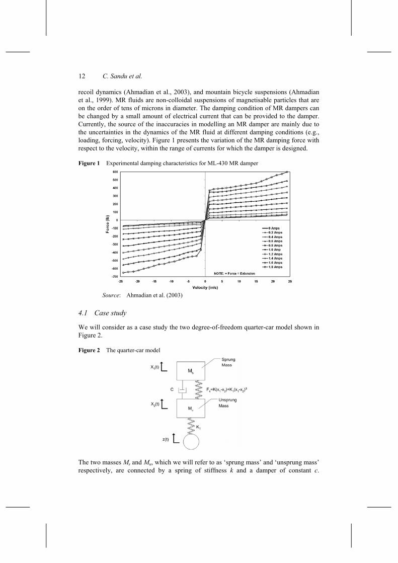
recoil dynamics (Ahmadian et al., 2003), and mountain bicycle suspensions (Ahmadian et al., 1999). MR fluids are non-colloidal suspensions of magnetisable particles that are on the order of tens of microns in diameter. The damping condition of MR dampers can be changed by a small amount of electrical current that can be provided to the damper. Currently, the source of the inaccuracies in modelling an MR damper are mainly due to the uncertainties in the dynamics of the MR fluid at different damping conditions (e.g., loading, forcing, velocity). Figure 1 presents the variation of the MR damping force with respect to the velocity, within the range of currents for which the damper is designed.

Figure 1 Experimental damping characteristics for ML-430 MR damper

Source: Ahmadian et al. (2003)

4.1 Case study

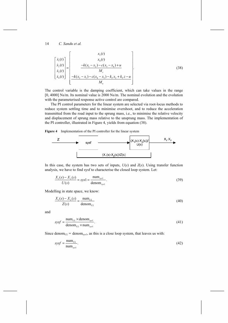
We will consider as a case study the two degree-of-freedom quarter-car model shown in Figure 2.

Figure 2 The quarter-car model

The two masses Ms and Mu, which we will refer to as ‘sprung mass’ and ‘unsprung mass’ respectively, are connected by a spring of stiffness k and a damper of constant c.

A response spectral decomposition approach 13

The forcing function is applied to Mu through the linear spring of stiffness kT, as z(t), where

( ) sin(2 ), 0.25 , 3 Hz.z t A ft A m fπ= = = (37)

The control variable was parameterised using Legendre polynomials of order up to 3. x1 and x2 are the sprung mass, and respectively the unsprung mass displacements. K1 is the stiffness of the suspension spring in the nonlinear (cubic) region.

We applied the control methodology proposed in this study on a linear test problem, and on a nonlinear test problem. In both cases the response of the system is analysed for various types of excitation input.

Figure 3 shows the response of the spring and of the damper for the linear and for the nonlinear test problems. For the nonlinear case, the spring has a cubic stiffness characteristic, and the response of the MR damper was modelled using a hyperbolic tangent function.

The response of the system controlled with traditional methods (PI, PID and Skyhook controllers) is compared in each case with the response of the system given by the parameterised response control.

Figure 3 Spring and damper response for linear and nonlinear test problems: (a) linear spring stiffness charact.; (b) cubic spring stiffness charact.; (c) linear damping coefficient charact. and (d) MR damping charact.

(a) (b)

(c) (d)

4.2 The linear test problem

First, we consider the quarter-car model with linear characteristics for the spring and for the damper that connect the sprung and the unsprung masses. The state-space representation of the system in this case is:

14 C. Sandu et al.

3

1 4

2 1 2 3 4

3

4 2 1 4 3 2

( )( ) ( )( ) ( ) ( )

.( )( ) ( ) ( )

s

T T

u

x tx t x tx t k x x c x x u

Mx tx t k x x c x x k x k z u

M

− − − − + = − − − − − + −

(38)

The control variable is the damping coefficient, which can take values in the range [0, 4000] Ns/m. Its nominal value is 2000 Ns/m. The nominal evolution and the evolution with the parameterised response active control are compared.

The PI control parameters for the linear system are selected via root-locus methods to reduce system settling time and to minimise overshoot, and to reduce the acceleration transmitted from the road input to the sprung mass, i.e., to minimise the relative velocity and displacement of sprung mass relative to the unsprung mass. The implementation of the PI controller, illustrated in Figure 4, yields from equation (38).

Figure 4 Implementation of the PI controller for the linear system

In this case, the system has two sets of inputs, U(s) and Z(s). Using transfer function analysis, we have to find sysf to characterise the closed loop system. Let:

11 2

1

num( ) ( ) 1 .( ) denom

sys

sys

X s X s sysU s

−= = (39)

Modelling in state space, we know:

1 2 num( ) ( )( ) denom

CL

CL

X s X sZ s

− = (40)

and

1

1

num denom.

denom numCL sys

CL sys

sysf×

=×

(41)

Since denomCL = denomsys1, as this is a close loop system, that leaves us with:

1

num .num

CL

sys

sysf = (42)

A response spectral decomposition approach 15

4.2.1 Sinusoidal excitation

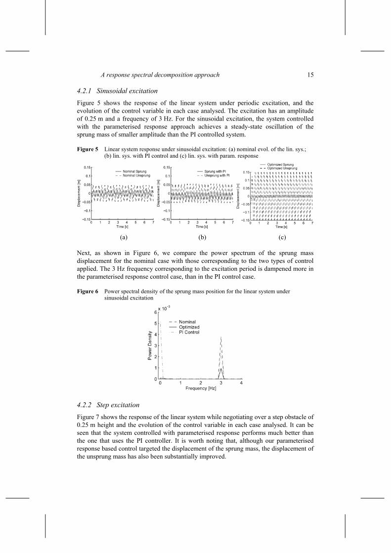
Figure 5 shows the response of the linear system under periodic excitation, and the evolution of the control variable in each case analysed. The excitation has an amplitude of 0.25 m and a frequency of 3 Hz. For the sinusoidal excitation, the system controlled with the parameterised response approach achieves a steady-state oscillation of the sprung mass of smaller amplitude than the PI controlled system.

Figure 5 Linear system response under sinusoidal excitation: (a) nominal evol. of the lin. sys.; (b) lin. sys. with PI control and (c) lin. sys. with param. response

(a) (b) (c)

Next, as shown in Figure 6, we compare the power spectrum of the sprung mass displacement for the nominal case with those corresponding to the two types of control applied. The 3 Hz frequency corresponding to the excitation period is dampened more in the parameterised response control case, than in the PI control case.

Figure 6 Power spectral density of the sprung mass position for the linear system under sinusoidal excitation

4.2.2 Step excitation

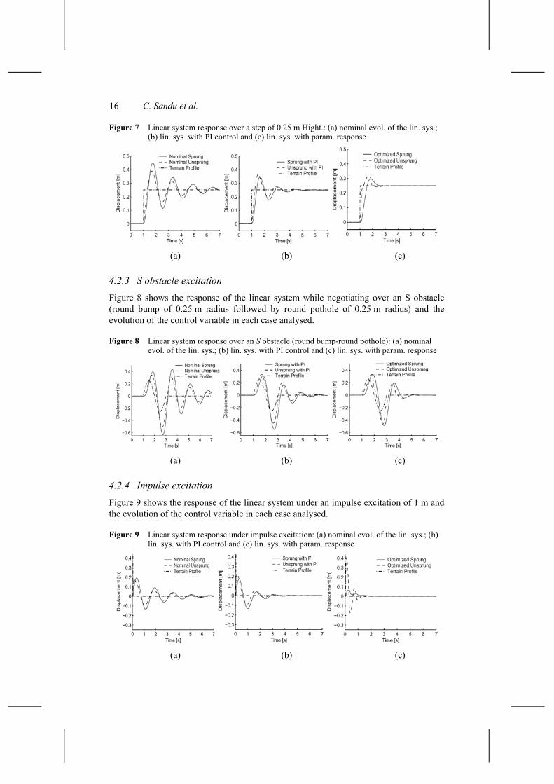
Figure 7 shows the response of the linear system while negotiating over a step obstacle of 0.25 m height and the evolution of the control variable in each case analysed. It can be seen that the system controlled with parameterised response performs much better than the one that uses the PI controller. It is worth noting that, although our parameterised response based control targeted the displacement of the sprung mass, the displacement of the unsprung mass has also been substantially improved.

16 C. Sandu et al.

Figure 7 Linear system response over a step of 0.25 m Hight.: (a) nominal evol. of the lin. sys.; (b) lin. sys. with PI control and (c) lin. sys. with param. response

(a) (b) (c)

4.2.3 S obstacle excitation

Figure 8 shows the response of the linear system while negotiating over an S obstacle (round bump of 0.25 m radius followed by round pothole of 0.25 m radius) and the evolution of the control variable in each case analysed.

Figure 8 Linear system response over an S obstacle (round bump-round pothole): (a) nominal evol. of the lin. sys.; (b) lin. sys. with PI control and (c) lin. sys. with param. response

(a) (b) (c)

4.2.4 Impulse excitation

Figure 9 shows the response of the linear system under an impulse excitation of 1 m and the evolution of the control variable in each case analysed.

Figure 9 Linear system response under impulse excitation: (a) nominal evol. of the lin. sys.; (b) lin. sys. with PI control and (c) lin. sys. with param. response

(a) (b) (c)

A response spectral decomposition approach 17

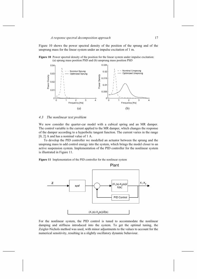
Figure 10 shows the power spectral density of the position of the sprung and of the unsprung mass for the linear system under an impulse excitation of 1 m.

Figure 10 Power spectral density of the position for the linear system under impulse excitation: (a) sprung mass position PSD and (b) unsprung mass position PSD

(a) (b)

4.3 The nonlinear test problem

We now consider the quarter-car model with a cubical spring and an MR damper. The control variable is the current applied to the MR damper, which changes the response of the damper according to a hyperbolic tangent function. The current varies in the range [0, 2] A and has a nominal value of 1 A.

To develop the PID controller we modelled an actuator between the sprung and the unsprung mass to add control energy into the system, which brings the model closer to an active suspension system. Implementation of the PID controller for the nonlinear system is illustrated in Figure 11.

Figure 11 Implementation of the PID controller for the nonlinear system

For the nonlinear system, the PID control is tuned to accommodate the nonlinear damping and stiffness introduced into the system. To get the optimal tuning, the Zeigler-Nichols method was used, with minor adjustments to the values to account for the numerical sensitivity, resulting in a slightly oscillatory dynamic behaviour.

18 C. Sandu et al.

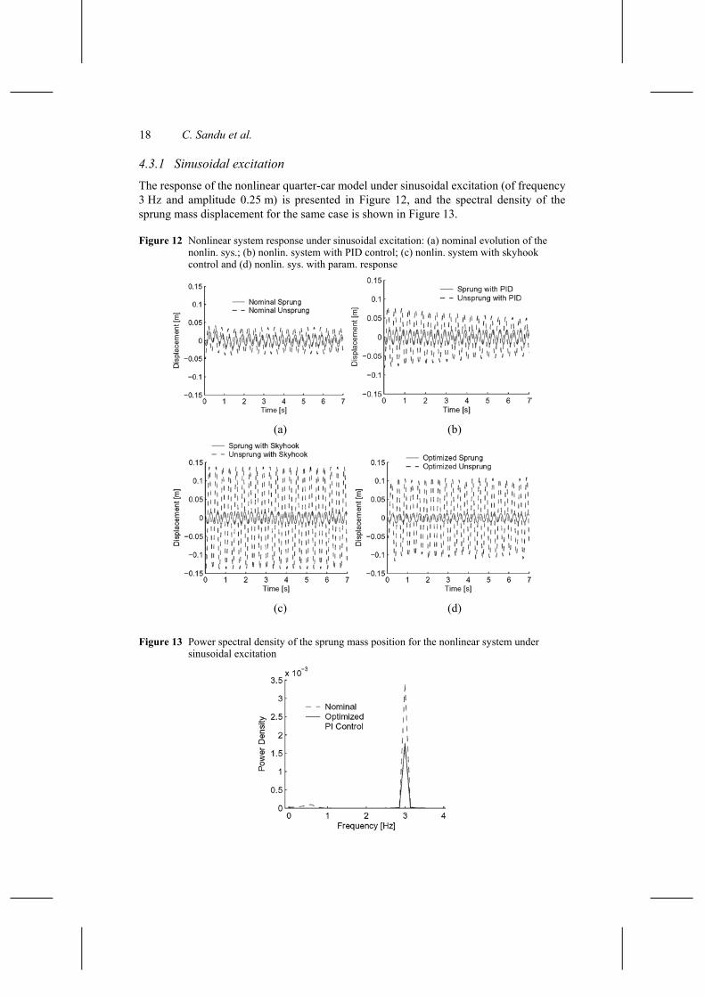
4.3.1 Sinusoidal excitation

The response of the nonlinear quarter-car model under sinusoidal excitation (of frequency 3 Hz and amplitude 0.25 m) is presented in Figure 12, and the spectral density of the sprung mass displacement for the same case is shown in Figure 13.

Figure 12 Nonlinear system response under sinusoidal excitation: (a) nominal evolution of the nonlin. sys.; (b) nonlin. system with PID control; (c) nonlin. system with skyhook control and (d) nonlin. sys. with param. response

(a) (b)

(c) (d)

Figure 13 Power spectral density of the sprung mass position for the nonlinear system under sinusoidal excitation

A response spectral decomposition approach 19

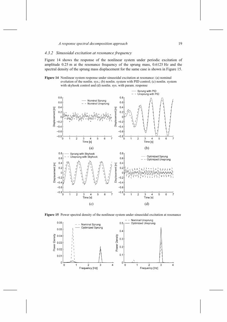
4.3.2 Sinusoidal excitation at resonance frequency

Figure 14 shows the response of the nonlinear system under periodic excitation of amplitude 0.25 m at the resonance frequency of the sprung mass, 0.6125 Hz and the spectral density of the sprung mass displacement for the same case is shown in Figure 15.

Figure 14 Nonlinear system response under sinusoidal excitation at resonance: (a) nominal evolution of the nonlin. sys.; (b) nonlin. system with PID control; (c) nonlin. system with skyhook control and (d) nonlin. sys. with param. response

(a) (b)

(c) (d)

Figure 15 Power spectral density of the nonlinear system under sinusoidal excitation at resonance

20 C. Sandu et al.

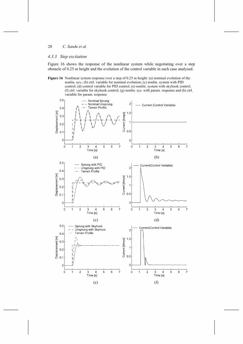
4.3.3 Step excitation

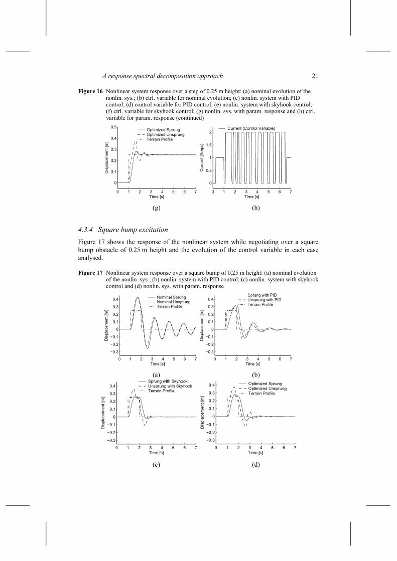
Figure 16 shows the response of the nonlinear system while negotiating over a step obstacle of 0.25 m height and the evolution of the control variable in each case analysed.

Figure 16 Nonlinear system response over a step of 0.25 m height: (a) nominal evolution of the nonlin. sys.; (b) ctrl. variable for nominal evolution; (c) nonlin. system with PID control; (d) control variable for PID control; (e) nonlin. system with skyhook control; (f) ctrl. variable for skyhook control; (g) nonlin. sys. with param. response and (h) ctrl. variable for param. response

(a) (b)

(c) (d)

(e) (f)

A response spectral decomposition approach 21

Figure 16 Nonlinear system response over a step of 0.25 m height: (a) nominal evolution of the nonlin. sys.; (b) ctrl. variable for nominal evolution; (c) nonlin. system with PID control; (d) control variable for PID control; (e) nonlin. system with skyhook control; (f) ctrl. variable for skyhook control; (g) nonlin. sys. with param. response and (h) ctrl. variable for param. response (continued)

(g) (h)

4.3.4 Square bump excitation

Figure 17 shows the response of the nonlinear system while negotiating over a square bump obstacle of 0.25 m height and the evolution of the control variable in each case analysed.

Figure 17 Nonlinear system response over a square bump of 0.25 m height: (a) nominal evolution of the nonlin. sys.; (b) nonlin. system with PID control; (c) nonlin. system with skyhook control and (d) nonlin. sys. with param. response

(a) (b)

(c) (d)

22 C. Sandu et al.

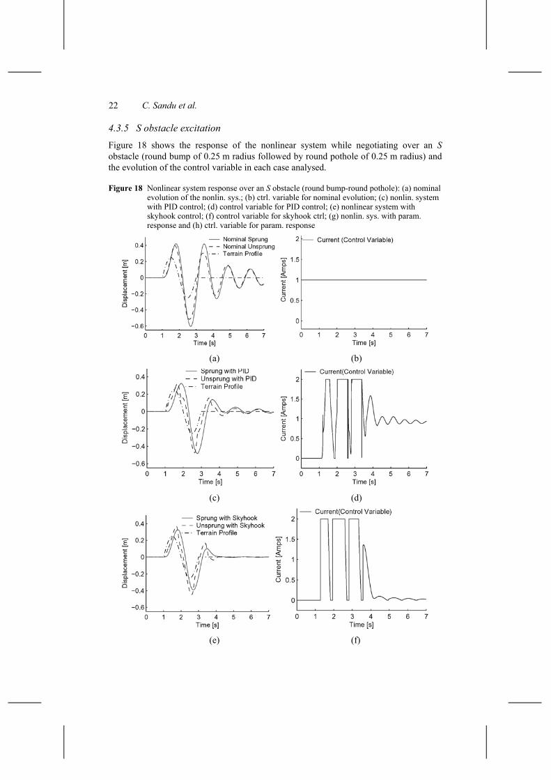
4.3.5 S obstacle excitation

Figure 18 shows the response of the nonlinear system while negotiating over an S obstacle (round bump of 0.25 m radius followed by round pothole of 0.25 m radius) and the evolution of the control variable in each case analysed.

Figure 18 Nonlinear system response over an S obstacle (round bump-round pothole): (a) nominal evolution of the nonlin. sys.; (b) ctrl. variable for nominal evolution; (c) nonlin. system with PID control; (d) control variable for PID control; (e) nonlinear system with skyhook control; (f) control variable for skyhook ctrl; (g) nonlin. sys. with param. response and (h) ctrl. variable for param. response

(a) (b)

(c) (d)

(e) (f)

A response spectral decomposition approach 23

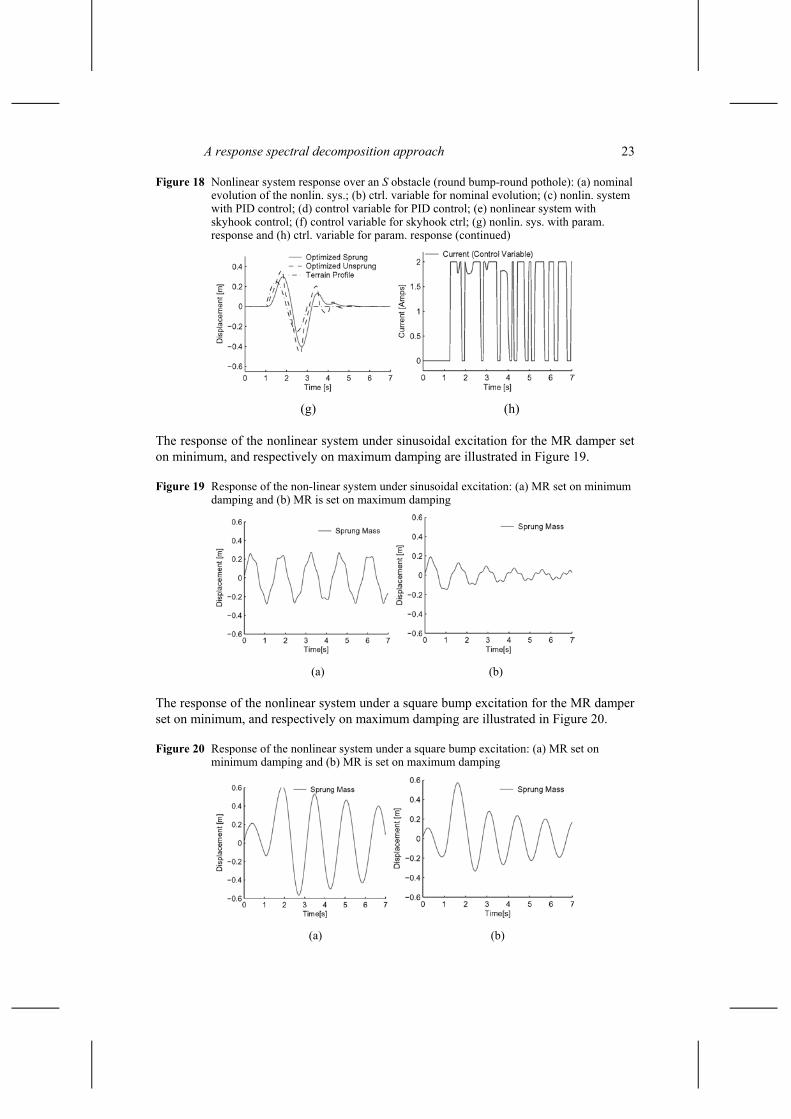
Figure 18 Nonlinear system response over an S obstacle (round bump-round pothole): (a) nominal evolution of the nonlin. sys.; (b) ctrl. variable for nominal evolution; (c) nonlin. system with PID control; (d) control variable for PID control; (e) nonlinear system with skyhook control; (f) control variable for skyhook ctrl; (g) nonlin. sys. with param. response and (h) ctrl. variable for param. response (continued)

(g) (h)

The response of the nonlinear system under sinusoidal excitation for the MR damper set on minimum, and respectively on maximum damping are illustrated in Figure 19.

Figure 19 Response of the non-linear system under sinusoidal excitation: (a) MR set on minimum damping and (b) MR is set on maximum damping

(a) (b)

The response of the nonlinear system under a square bump excitation for the MR damper set on minimum, and respectively on maximum damping are illustrated in Figure 20.

Figure 20 Response of the nonlinear system under a square bump excitation: (a) MR set on minimum damping and (b) MR is set on maximum damping

(a) (b)

24 C. Sandu et al.

5 Conclusions and future work

This paper discusses a control methodology for dynamic systems based on explicitly characterising all possible system responses to all possible values of the control variables.

The proposed approach is to extend the dynamic model along the parameterised control dimension. This allows a representation of the state of the system which explicitly depends on both time and control variables. The underlying idea is to extend the system along the ‘control dimension’ and explicitly account for the dependence of the system state on control variables. A spectral discretisation along the ‘control dimension’ is employed.

The construction of the evolution equations for the spectral coefficients is discussed in both the Galerkin and collocation frameworks. Multibody dynamic systems typically display two types of nonlinearities, polynomial and trigonometric. In the Galerkin approach the evaluation of multi-dimensional integrals is needed to compute inner products. It is shown that the tensor product nature of basis functions makes the evaluation of inner products computationally efficient for polynomial nonlinearities. However, for trigonometric nonlinearities multi-dimensional integration is required, and this can be accomplished using numerical quadrature rules. Spectral collocation only requires the evaluation of functions at different collocation points. It can be easily applied to any type of nonlinearities and does not require recoding of the original model of the system of interest.

The time interval of interest is divided in subintervals, on which the control variables are kept constant. The system response over each subinterval is obtained by integrating the extended system. The control values for the subinterval are the solutions of an optimisation problem. The cost function is formulated in terms of the parameterised system response.

We present numerical results for linear and nonlinear quarter-car models riding over different terrain profiles. The new control strategy is compared against well established control methods. The response of the system shows good performance and is comparable with the response of the system with the more traditional control methods. The results are promising, as the proposed approach is general and can be applied to any dynamical system.

Future research directions in this area include the study of systems with multiple control variables, and applications to MR dampers and realistic vehicle models. We will consider system response parameterisations in terms of Chebyshev polynomials. This representation will allow a better point-wise approximation (near mini-max approximation) of the system response.

References Ahmadian, M., Appleton, R. and Norris, J.A. (1999) ‘Design and development of

magneto-rheological dampers for bicycle suspensions’, ASME Int. Congress and Exposition, Nashville, TN.

Ahmadian, M., Appleton, R. and Norris, J.A. (2003) ‘Designing magneto-rheological recoil dampers in a fire-out-of battery recoil system’, IEEE Transactions on Magnetics, Vol. 39, No. 1, pp.480–485.

Dorf, R.C. and Bishop, R.H. (2001) Modern Control Systems, 9 ed., Prentice-Hall, NJ.

A response spectral decomposition approach 25

Dyke, S.J., Spencer Jr., B.F., Sain, M.K. and Carlson, J.D. (1996) ‘Seismic Response reduction using magnetorheological dampers’, IFAC World Congress, San Francisco, CA.

Ghanem, R. and Spanos, P. (1991a) Stochastic Finite Elements: A Spectral Approach, Springer-Verlag, Berlin and New York.

Ghanem, R. and Spanos, P. (1991b) A Spectral Stochastic Finite Element Formulation for Reliability Analysis. ASCE, Vol. 117, No. 10, pp.2351–2372.

Gordaninejad, F. and Kelso, S.P. (2000) ‘Magneto-rheological fluid shock absorbers for HMMWV’, in Tupper Hyde, T. (Ed.): Smart Structures and Materials 2000: Damping and Isolation, Proc. SPIE, Vol. 3989, pp.266–273.

Gottlieb, D. and Orszag, S.A. (1987) Numerical Analysis of Spectral Methods: Theory and Applications, SIAM.

Isukapalli, S.S., Roy, A. and Georgopoulos, P.G. (1998) ‘Stochastic response surface methods (SRSMs) for uncertainty propoagation: application to environmental and biological systems’, Risk Analysis, Vol. 18, No. 3, pp.351–363, doi:10.1111/j.1539-6924.1998.tb01301.x.

Tatang, M.A., Pan, W., Prinn, R.G. and McRae, G.J. (1997) ‘An efficient method for parametric uncertainty analysis of numerical geophysical models’, J. Geophy. Res., Vol. 102, pp.21925–21932.

Trefethen, L.N. and Baw, D. (1998) III Spectral Methods in MATLAB, SIAM. Xiu, D. and Karniadakis, G.E. (2002) ‘The Wiener-Askey polynomial chaos for stochastic

differential equations’, SIAM J. Sci. Comput., Vol. 24, No. 1, pp.619–644.

Appendix A: Basis functions

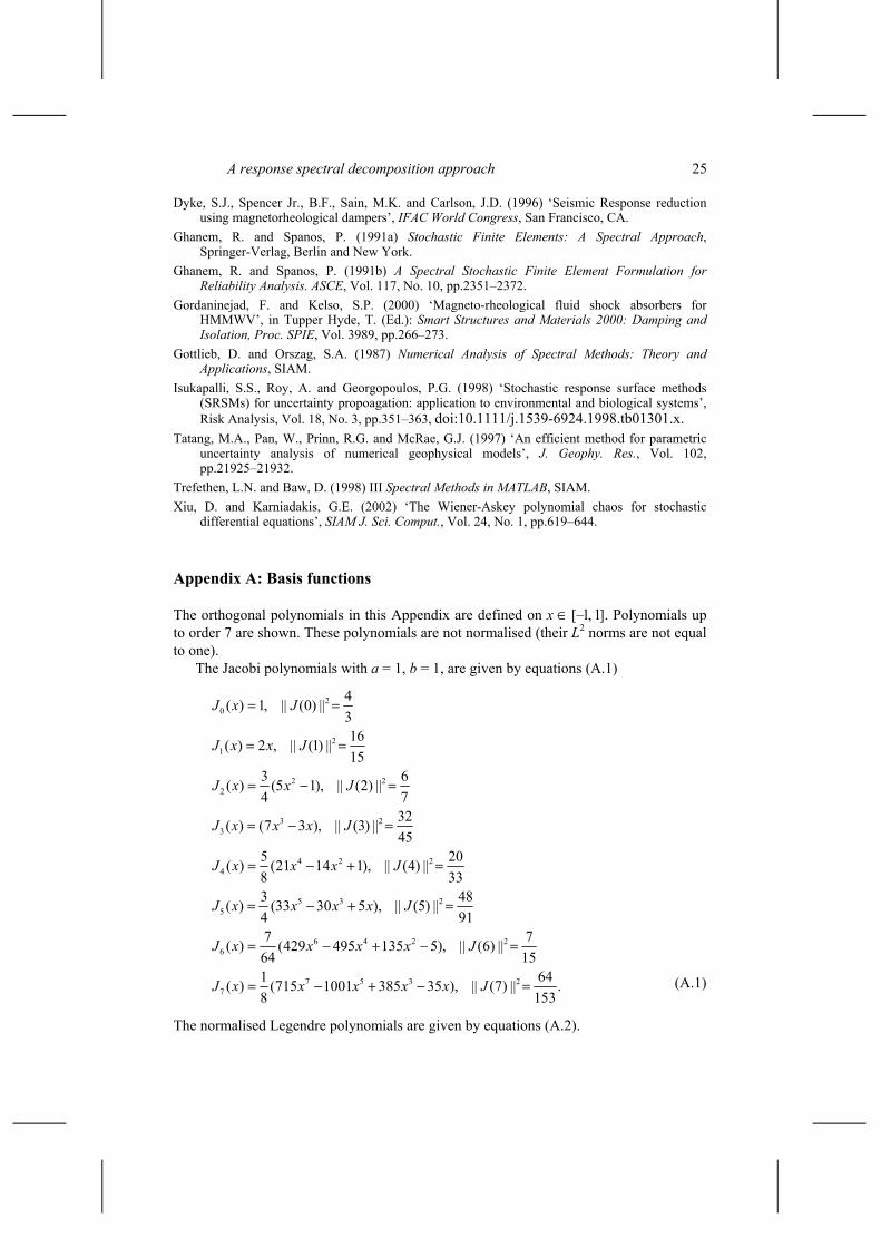
The orthogonal polynomials in this Appendix are defined on x ∈ [–l, l]. Polynomials up to order 7 are shown. These polynomials are not normalised (their L2 norms are not equal to one).

The Jacobi polynomials with a = 1, b = 1, are given by equations (A.1)

20

21

2 22

3 23

4 2 24

5 3 25

6 4 26

4( ) 1, || (0) ||316( ) 2 , || (1) ||15

3 6( ) (5 1), || (2) ||4 7

32( ) (7 3 ), || (3) ||45

5 20( ) (21 14 1), || (4) ||8 333 48( ) (33 30 5 ), || (5) ||4 917( ) (429 495 13564

J x J

J x x J

J x x J

J x x x J

J x x x J

J x x x x J

J x x x x

= =

= =

= − =

= − =

= − + =

= − + =

= − + 2

7 5 3 27

75), || (6) ||15

1 64( ) (715 1001 385 35 ), || (7) || .8 153

J

J x x x x x J

− =

= − + − = (A.1)

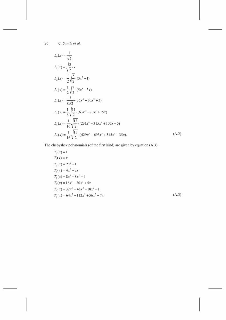
The normalised Legendre polynomials are given by equations (A.2).

26 C. Sandu et al.

0

1

22

33

4 24

5 35

6 46

7 5 37

1( )23( )2

1 5( ) (3 1)2 21 7( ) (5 3 )2 2

3( ) (35 30 3)8 21 11( ) (63 70 15 )8 21 13( ) (231 315 105 5)

16 21 15( ) (429 693 315 35 ).

16 2

L x

L x x

L x x

L x x x

L x x x

L x x x x

L x x x x

L x x x x x

=

= ⋅

= ⋅ −

= ⋅ −

= ⋅ − +

= ⋅ − +

= ⋅ − + −

= ⋅ − + − (A.2)

The chebyshev polynomials (of the first kind) are given by equation (A.3):

0

12

23

3

4 24

5 35

6 4 26

7 5 37

( ) 1( )

( ) 2 1( ) 4 3

( ) 8 8 1( ) 16 20 5

( ) 32 48 18 1

( ) 64 112 56 7 .

T xT x x

T x xT x x x

T x x xT x x x x

T x x x x

T x x x x x

==

= −

= −

= − +

= − +

= − + −

= − + − (A.3)