Embed Size (px)
Citation preview
Zeta: a Resolution Modeling System
P. Cignoni�, C. Montaniy, C. Rocchiniz, R. Scopignox
Istituto per l'Elaborazione dell'Informazione { Consiglio Nazionale delle Ricerche
Via S. Maria, 46 - 56126 Pisa ITALY
�Email: [email protected]
yEmail: [email protected]
zEmail: [email protected]
xEmail: [email protected]
May 20, 1998
Abstract
Very large graphics models are common in a number of applications, and many di�erent simpli�-
cation methods have been recently developed. Some of them support the construction of multireso-
lution representations of the input meshes. On the basis of these innovative techniques, we foresee a
modeling framework based on three separate stages (shape modeling, multiresolution encoding and
resolution modeling), and propose a new approach to the last stage, resolution modeling, which is
highly general, user-driven and not strictly tied to a particular simpli�cation method.
The approach proposed is based on a multiresolution representation scheme for triangulated, 2-
manifold meshes, the Hypertriangulation Model (HyT). This scheme allows to selectively \walk"
along the multiresolution surface, moving between adjacent faces e�ciently. A prototypal resolution
modeling system, Zeta, has been implemented to allow interactive modeling of surface details and
evaluated on several practical models. It supports: e�cient extraction of �xed resolution representa-
tions; uni�ed management of selective re�nement and selective simpli�cation; easy composition of the
selective re�nement/simpli�cation actions, with no cracks in the variable resolution mesh produced;
multiresolution editing; interactive response times.
CR Descriptors: I.3.5 [Computer Graphics]: Computational Geometry and Object Modeling
- Curve, surface, solid and object representation; I.3.6 [Computer Graphics]: Methodology and
Techniques.
Additional Keywords: surface modeling, mesh simpli�cation, multiresolution, selective re�ne-
ments, resolution modeling.
Contact person:
Roberto Scopigno, I.E.I.- C.N.R.,
Via S. Maria 46, 56126 PISA (Italy)
Phone: +39 50 593304 FAX: +39 50 904052
EMail: [email protected]
1
1 Introduction
Multiresolution representation is a very hot topic, due to the increasing complexity of virtual graphic
worlds. Huge models are produced in a number of applications, e.g. terrain modeling, volume visualiza-
tion, virtual reality, automatic modeling based on range scanners, free form surface modeling. Models
are usually speci�ed with [triangle-based] surface meshes, and nowadays a key issue is how to store,
access and visualize in real time hundreds of thousands of faces. Many methods for the simpli�cation of
geometrical information have appeared in the last few years. A direct consequence was the proposal of
the Level of Detail (LoD) paradigm { a conceptual model where an object is stored through a constant
number k of di�erent representations, each of them at a di�erent level of detail or approximation [5].
LoD are usually adopted to speedup visualization, because simpli�ed representations are su�cient for a
large percentage of possible views [14, 18].
But LoD is neither the only nor the most sophisticated way to manage multiresolution. At this point
we would like to use the term multiresolution (or continuous LOD) for only those data structures which
allow the compact representation of a number m of representations, at di�erent levels of detail, where m
is not constant but is a monotone function of the data size (e.g., of the number of faces in the represented
surface mesh). In other words, a multiresolution representation is not the simple collection of a [small]
number of prede�ned models, but a compact representation of shape details plus the algorithms which
allow an on-the- y reconstruction of each possible level of detail representation [19, 2, 1, 31].
Multiresolution has been adopted at �rst to increase graphic throughput [14, 3], but di�erent appli-
cations can be devised. Terrain visualization is one of the early �elds of application of multiresolution
modeling [7, 23, 4, 20, 10], e.g. to build dynamically variable resolution representations, which link
resolution to the importance in viewing space of each projected parcel (e.g. a single terrain patch).
In this paper we try to extend the domain of possible applications. Rather than simply taking into
account the viewing space \impact" of the represented data, a variable resolution representation of an
object can be conceived as a user-driven interpretation on the object itself, optimized to convey a given
amount of knowledge. For this reason we believe that resolution modeling has a strong similarity with
shape modeling, in the sense that it has to be ful�lled through a tight interaction with the user. While the
construction of the multiresolution representation is a process which can be simply made in an automatic
and unattended way, the resolution modeling phase generally involves an interpretation of the data which
cannot be ful�lled without human intervention.
Given this framework, the rationale of this paper is to propose a new data structure and algorithms
which allow the user to add/remove resolution to localised parts of a model. Standard CAD systems
provide tools to assist users in the design of \shapes", but none of them actually provide the tools needed
to manage what we would conceive as a second-stage modeling session: given a �rst stage in which the
\shape" is designed/scanned in full detail, then we want to allow the user to play with resolution to build
di�erent instances of the the input shape which are characterised by variable resolutions/details. Our
global modeling conceptual model is therefore characterised by three phases as follows:
1. shape modeling, the canonical three-dimensional shape modeling (via CAD design, range scan
acquisition or isosurface �tting);
2. multiresolutionmodel construction, recent surface simpli�cationmethods [2, 19] easily support
this phase;
2
3. resolution modeling, user-driven modeling of variable resolution representations of the given
shape.
Our goal is therefore to design an interactive tool which provides the user with selective and incremental
resolution modeling features. This tool, called Zeta, adopts a multiresolution representation for triangu-
lated, orientable, 2-manifold surfaces in 3D space, which allows compact storing and e�cient navigation
over a multiresolution mesh. We propose with Zeta a new methodology for the uni�ed management of
selective re�nements and selective simpli�cation (i.e., either increasing or reducing the mesh detail locally
on mesh subareas chosen by the user). This selective re�nement/simpli�cation operator has been im-
plemented via the e�cient navigation over the multiresolution representation, which allows partial mesh
updates and guarantees C0 continuity (i.e. no cracks) on each intermediate variable resolution mesh.
In the Zeta system framework, resolution modeling is achieved with the following steps:
LOAD a multiresolution representation of the mesh;
SELECT a representation at a �xed level of resolution;
LOOP
[ user: select the radius of the current region of interest ]
[ user: toggle between re�nement/simpli�cation; ]
[ user: modify the current Error propagation function; ]
user: pick the mesh to select the current action focus point;
Zeta: perform a selective re�nement/simpli�cation action on the
current variable resolution mesh;
UNTIL completion of variable resolution mesh modeling.
Resolution Modeling Applications
We believe that resolution modeling is a very general methodology. Consequently, the potential applica-
tion domain is broad, and in the following we only glance to some possible uses. We subdivide resolution
modeling applications into two broad classes: those where resolution modeling can be managed in an
unattended, computer{driven manner, and those which have to be operated under strict user control.
Computer-driven applications have been recently proposed, to construct variable resolution terrain mod-
els for ight simulators [7, 23, 20, 4], or to build dynamic LoD [31, 20]. Variable resolution meshes are
produced in this applications by taking into account the current view speci�cations.
Much less studied are the possible user-driven applications, such as:
� the editing of shapes acquired via range scanners or other automatic acquisition devices/algorithms.
Direct acquisition produces highly detailed shapes and the standard simpli�cation codes operate on
these meshes using the same criterion on the whole mesh, generally a user-de�ned approximation
threshold. But real applications may need to apply a variable threshold on the mesh. Let us
consider human body acquisition: high precision is generally required for the face or the hands of
the subject (perhaps in the range of one millimetre or less), while a much larger threshold may be
imposed on less important areas such as the legs or the torso;
� the design of characters in computer-based animation. Each single character may be speci�ed in
terms of n di�erent variable resolution representations, which are built to take care of di�erent
presentation contexts (e.g. a foreground character which is either half length or full length);
3
� the production of assembly instructions for 3D compound objects or systems. To produce illustra-
tions or animated sequences of an assembly, often the entire and highly complex description of each
subcomponent is not needed or even counterproductive. A variable resolution representation may
be adopted to convey a complete description of only the surface section that play a major role in
the current assembly action, therefore enhancing the cognitive importance of the most detailed part
and reducing both image cluttering and rendering times. An example of the use of two di�erent
rendering modes, to enhance the di�erent information given to the user, is presented in Figure 12;
the choice among the two rendering modes (shaded or edge only) is driven by surface resolution.
Paper organization. Section 2 brie y reviews the state of the art in surface simpli�cation and mul-
tiresolution representation. Section 3 describes how a multiresolution model, i.e. the Zeta input data,
can be constructed, starting from classical incremental simpli�cation or re�nement approaches. The in-
novative contributions of the paper are presented in Section 4: we introduce the compact and e�cient
multiresolution data representation scheme (Subsection 4.1), its initialization for multiresolution data
loading (Subsection 4.2), and the selective re�nement/simpli�cation algorithm (Subsection 4.3). Simple
features for editing the multiresolution mesh are sketched in Section 5. An evaluation of the proposed
methodology is presented in Section 6. Finally, conclusions are drawn in Section 7.
2 Previous work
Many approaches have been proposed to reduce the complexity of surface meshes [24]. They may be
classi�ed, at a high level of abstraction, into two main classes. Re�nement heuristics start from a model
(usually based on a simplicial complex) whose vertices are a very small subset of the input dataset S and
iteratively insert vertices in the mesh, until the model satis�es the required precision [13]. Simpli�cation
heuristics start from the input model and iteratively reduce complexity, by discarding as many elements
as possible, while maintaining the required precision. Many di�erent simpli�cation approaches have been
proposed, based onmesh decimation [28, 6, 25, 2],mesh optimization [21, 19], re{tiling [29],multiresolution
analysis [11], and vertex clustering [26, 16].
An LoD representation may be simply built by the iterative application of any of the simpli�ca-
tion/re�nement approaches above, while only few of them propose the construction of multiresolution
mesh representations [19, 2, 11]. The LoD paradigm has been incorporated in recent libraries or toolkits
for 3D graphics, e.g. OpenInventor and VRML, and in some solid modellers or scene editors. The inher-
ent limitations with the current implementations of the LoD paradigm are the limited number (generally
very few) of di�erent approximations which are stored, to reduce redundancy and space occupancy, and
the non dynamic nature of the representation itself. The represented levels are generally built in a pre{
processing step, to allow the fastest access to data in rendering. But the selection of the resolution would
ideally depend on dynamic parameters, e.g. to ensure data-independent constant frame rates. This is
obviously the case of digital terrains visualization; multiresolution digital terrain models have been re-
viewed in a recent paper by De Floriani and Puppo [8]. Methods for the construction of multiresolution
representations of generic surfaces in IR3 have been proposed by adopting classical face-based approaches
[31, 20, 2, 32] or wavelet{based approaches [11, 17, 1].
A seminal work on local re�nement and multiresolution modeling, which somehow anticipated what we
propose in this paper, was proposed by Forsey and Bartels [12]. They designed a system for locally
re�ning surfaces represented with hierarchical B-splines.
4
LoD or multiresolution representations have been adopted in many applications: to reduce rendering
time in visualization [14, 3, 30, 27, 7, 31, 4, 8, 23, 10]; to apply progressive transmission of 3D meshes
on low bandwidth lines [19, 1]; to implement selective re�nements or multiresolution editing on surfaces
[7, 19, 20, 32].
In particular, multiresolution data structure have been proposed to allow the dynamic extraction of
view-dependent variable resolution meshes. Xia and Varshney [31] proposed the merge tree structure
which encodes in a binary tree all of the allowed vertex collapse actions and the dependencies between
these actions. To extract a variable resolution mesh, the merge tree is visited recursively bottom-up to
�nd all of the vertices that have to be included in the output mesh (e.g. by evaluating a criterion based
on the size in view coordinates of the split edge). The set of triangles corresponding to these vertices
may be computed from scratch by starting from the high resolution mesh and progressively collapsing
edges, or by computing the current mesh Mi from the mesh Mi�1 taking into account frame{to{frame
coherence.
Whereas the merge tree representation is based on edge lengths and constrain the hierarchy to a set
of levels with non overlapping collapsing fragments, the Hoppe's progressive meshes approach [19, 20]
lets the hierarchy be formed by an unconstrained, geometrically optimized sequence of vertex splitting
transformations, and introduces as few dependencies as possible between these transformations, in order
to minimize the complexity of the extracted meshes. On this data structure, Hoppe de�nes a dynamic
re�nement function which determines whether each single vertex has to be re�ned, based on current
view parameters (a re�nement is applied only if the vertex to be split is in the view frustum, if adjacent
faces are not back-oriented, and if the associated screen-space geometric error is higher than a prede�ned
tolerance).
An interactive multiresolution mesh editing approach [32] was proposed with an objective somehow
similar to our: to increase usability and e�ciency of a modeling system by adopting a multiresolution
representation of the meshes. The user manipulates high resolution geometry as if working in a patch-
based system, with the additional bene�t of hierarchical editing semantics. Using sophisticated adaptive
subdivision techniques coupled with lazy evaluation, a scalable editing system has been de�ned. Through
the use of subdivision and smoothing techniques the system supports large scale smooth edits as well
as tweaking detail at the individual vertex level, while maintaining a concise internal representation
(based on a forest of triangle quadtrees). But because the representation is based on quartic triangle
re�nements, an inherent limitation of this approach is that the input mesh must possess subdivision
connectivity; otherwise it has to be re-meshed.
Unlikely previous multiresolution data structures [31, 20, 32], our multiresolution scheme is the only
one which explicitly stores topological information between the fragments that compose the multiresolu-
tion mesh, and which allows \walking" on the multiresolution surface, moving e�ciently between adjacent
faces (which may have the same or a \compatible" approximation error).
3 Construction of a multiresolution model
A surface mesh S may be simpli�ed by following either an incremental re�nement or simpli�cation
strategy. In both cases, a multiresolution output may be simply built if a global errormeasure is evaluated
after each local modi�cation action. In the following we take into account a simpli�cation heuristic based
on vertex decimation, but the same holds for other incremental simpli�cation or re�nement heuristic as
5

well.
Given a simpli�cation approach based on vertex removal, we call: S, the input mesh; Si, an intermediate
mesh obtained after i steps of the simpli�cation process; v the vertex candidate for removal on mesh Si;
Tv the patch of triangles in Si incident with v; and, �nally, T 0vthe new triangulation which will replace
Tv in Si+1 after the elimination of v.
At each step, we evaluate the global error of the current mesh Si, with respect to the original input
mesh S. Incremental simpli�cation approaches which adopt a global estimate of the error are available
[2, 22, 25, 16].
If we consider all surfaces built at intermediate simpli�cation steps, we have a whole sequence of triangu-
lations fS0; : : : ; Sng, where S0 is the input triangulation S, and 8i = 0; : : : ; n, the surface Si approximates
the full resolution mesh with an error "i. The only constrain imposed on the simpli�cation code is that
the sequence of error tolerances "i should increase monotonically: "0 = 0 < "1 < : : : < "n. Moreover, the
slower and smoother the growth of the approximation error is, the larger are the number and the quality
of the di�erent resolution meshes stored in the multiresolution model [2].
Let us consider the set T � of all the triangles that were generated during the entire decimation process,
including the triangles of the original mesh. Each facet t 2 T � is characterised by two errors: error at
creation time (or birth error, the error of the current mesh Si when t was generated as part of a new
patching sub-mesh) and error at elimination time (or death error, the error of the current mesh Si when
t was found as one of the triangles incident on a vertex being removed). Each facet t 2 T � is therefore
tagged by these two errors "b and "d, with "b < "d. The interval bounded by these two errors is called
life interval.
A straightforward multiresolution representation of the output produced by a simpli�cation algorithm is
therefore the list T �, with the "b and "d errors associated to each facet t 2 T �. This historical represen-
tation, called history for short, consists of two lists:
� vertex list { for each vertex vi, its [x,y,z] coordinates;
� face list { for each face fi: three indices to its vertices and its life interval d"b; "d].
The history avoids the replication of all the triangles which belong to more than one �xed resolution
mesh (or layer), and yelds an improvement in terms of memory space occupancy over the layered models
(e.g. LoD or other hierarchical layer-based structures). A prototypal decimator [2] which returns in
output a multiresolution mesh and uses the history data format is available on the web1.
The extraction from the history of a representation S" at a given precision " is straightforward: S" is
composed of all of the faces in the history such that their life interval contains the error threshold searched
for ("b � " < "d).
But the history representation is not su�cient when more sophisticated accesses to the multiresolution
data have to be managed. To support the e�cient implementation of a selective re�nement operator, a
more sophisticated multiresolution mesh representation is proposed in the following section.
4 Resolution Modeling
This section describes the data structures and the kernel functionalities of Zeta, our prototypal resolution
modeling system. The key functionality is to support selective re�nement or simpli�cation actions. Each
1See URL: http://miles.cnuce.cnr.it/cg/enhadecimation.html
6
Vertex Decimation
Patch Glueing
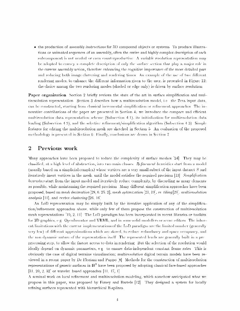
Figure 1: The Hypertriangulation (HyT) multiresolution scheme: the patches associated with a single
simpli�cation step (based on vertex decimation) are \glued" onto the common border.
action modi�es incrementally the current mesh by increasing/decreasing the resolution on a sub-area of
the mesh which is interactively selected by the user. It has to be performed in interactive time, and it
must guarantee C0 continuity on each intermediate result (the current output mesh).
Being the process user-driven, a complex dialog session has to be managed. The user has control over:
� the focus point pf on the current mesh;
� the current radius r, which identi�es the area size (to be re�ned/simpli�ed) surrounding pf on the
current mesh.
� the action (re�nement or simpli�cation) that has to be operated and the error function E which
determines, for each element of the mesh, the required increase/decrease of precision by taking into
account the distance of the element from pf .
According to user inputs, the system modi�es locally the current mesh, by decreasing or increasing the
mesh precision in the mesh subsection of radius r and centred in pf .
The interface of Zeta2 is presented in Figure 8. Six di�erent stages of a resolution modeling session
are presented in Figure 9, to highlight some of Zeta's capabilities. The mesh colors in the second, third
and fourth clips represent the error of each mesh face (using a color ramp from blue to red).
4.1 The Hypertriangulation scheme
This section introduces a multiresolution scheme for orientable, 2-manifold surfaces in IR3, called Hy-
pertriangulation (HyT) [4]. The scheme is general and can be adopted to store multiresolution output
produced either by simpli�cation or re�nement algorithms. For the sake of simplicity, hereafter we will
only consider simpli�cation algorithms.
We start from the history (see Section 3), and build a new representation to encode explicitly the
adjacencies between facets which share an edge, either in the same triangulation Si or in di�erent triangu-
2The �rst release of Zeta is available on the World Wide Web at address http://miles.cnuce.cnr.it/cg/zeta.html
7
v1
v2
f0
f1
f2
e1 e2
facet-edge f2e
1
facet-edge f1e
1
facet-edge f0e1
f4e2 f4
vert
f0
f1
f2
e1
packed-facet-edge e1
fother
enext[2]enext[1]enext[0]
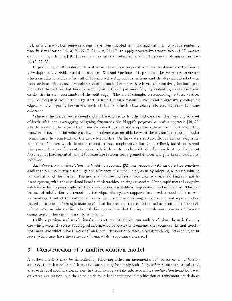
Figure 2: On the left, the original implementation of the HyT based on facet-edges, (one facet-edge record
for each face-edge pair); on the right, the new packed facet edge representation (a single record for all of
the facets on the same side of the oriented edge).
lations. Single triangulations (i.e. meshes at �xed approximation "i) are not explicitly and independently
stored in our structure, but we provide tools to reconstruct them e�ciently at run time.
Let us consider the re�nement region that is simpli�ed in passing from Si�1 to Si. The simpli�cation
action operated onto Si�1 de�nes two patches: the removed patch, i.e. the triangles in Si�1 incident on
the vertex to be removed; and the new patch, i.e. the triangles which re-triangulate the resulting hole. By
de�nition, the two sets of triangles share the edges that bound the current simpli�cation region. Hence,
instead of simply replacing the removed patch, we \glue" along such boundary edges the new patch over
the old one. In order to clarify the organization of the data, let us use a metaphor: we represent \visually"
the adjacency between patches by representing a new patch as a curved bubble which shares with the
removed one the chain of border edges (Figure 1). We can imagine that the resulting multiresolution data
structure is built by warping each new patch of a delta value su�cient to contain the removed patch, and
by welding it onto the old triangulation at the boundary of the old patch. The single simpli�cation step
is therefore visually represented as a new \bubble" glued onto the old patch.
The resulting structure can be topologically (but not geometrically) interpreted as a 3D subdivision of the
space (where a 3D cell corresponds to each bubble). This because geometry (i.e. vertices coordinates) is
not modi�ed at all.
The HyT multiresolution scheme follows the metaphors above. It maintains in a compact format both
the topological information, collected during the re�nement process, and the information on the error of
each triangle. The HyT scheme is encoded by adopting a packed facet-edge (pfe) representation. With
respect to its original design [4] (based on the facet-edge representation), the current HyT implementation
is more compact and more e�cient, because the lower redundancy allows faster implementation of critical
traversal functions.
The pfe has been designed as a modi�cation of the facet-edge, a data structure originally introduced for
the representation of 3D space subdivisions [9]. In the facet-edge scheme (see Figure 2.left), an atomic
entity is associated with each pair that is identi�ed by a face f and one of its edges e: the so-called
facet-edge. Each facet-edge denotes two rings: the edge-ring, composed by all the edges of the boundary
of f ; and the facet-ring, composed by all the faces incident at e. This structure is equipped with traversal
functions that enable the complex to be visited. These functions are used to move from a facet-edge to
an adjacent one, either by changing edge or by changing face (note that since our multiresolution model
8
is topologically equivalent to a 3D subdivision, more than two faces may be incident at each edge).
Instead of having a single facet{edge for each edge{face pair [4], the pfe representation encodes into
a single record all of the facet-edges incident on a given oriented edge from one of its sides (see Fig-
ure 2.right). Each pfe stores both geometrical and topological information related to the oriented edge
and to the faces sharing it. The data structures that implement the HyT scheme are therefore composed
of three entities: the Vertex, the Face and the PackedFacetEdge record.
The Vertex record holds the vertex coordinates plus two more �elds (the distance of the vertex from the
current focus point and a mark �eld), whose usage will be clari�ed in the following.
The Face record holds the life interval of the associated face ("b and "d values) and a mark �eld, which
is used as an incremental counter by the Selective Re�nement algorithm.
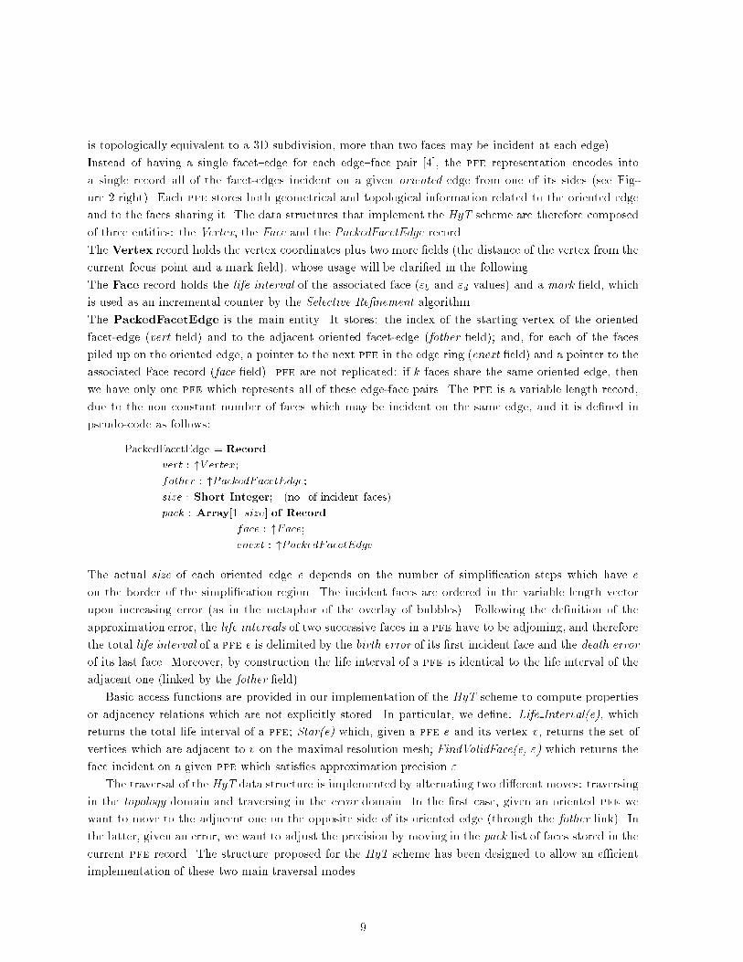
The PackedFacetEdge is the main entity. It stores: the index of the starting vertex of the oriented
facet-edge (vert �eld) and to the adjacent oriented facet-edge (fother �eld); and, for each of the faces
piled up on the oriented edge, a pointer to the next pfe in the edge ring (enext �eld) and a pointer to the
associated Face record (face �eld). pfe are not replicated: if k faces share the same oriented edge, then
we have only one pfe which represents all of these edge-face pairs. The pfe is a variable length record,
due to the non constant number of faces which may be incident on the same edge, and it is de�ned in
pseudo-code as follows:
PackedFacetEdge = Record
vert : "V ertex;
fother : "PackedFacetEdge;
size : Short Integer; (no. of incident faces)
pack : Array[1..size] of Record
face : "Face;
enext : "PackedFacetEdge
The actual size of each oriented edge e depends on the number of simpli�cation steps which have e
on the border of the simpli�cation region. The incident faces are ordered in the variable length vector
upon increasing error (as in the metaphor of the overlay of bubbles). Following the de�nition of the
approximation error, the life intervals of two successive faces in a pfe have to be adjoining, and therefore
the total life interval of a pfe e is delimited by the birth error of its �rst incident face and the death error
of its last face. Moreover, by construction the life interval of a pfe is identical to the life interval of the
adjacent one (linked by the fother �eld).
Basic access functions are provided in our implementation of the HyT scheme to compute properties
or adjacency relations which are not explicitly stored. In particular, we de�ne: Life Interval(e), which
returns the total life interval of a pfe; Star(e) which, given a pfe e and its vertex v, returns the set of
vertices which are adjacent to v on the maximal resolution mesh; FindValidFace(e, ") which returns the
face incident on a given pfe which satis�es approximation precision ".
The traversal of the HyT data structure is implemented by alternating two di�erent moves: traversing
in the topology domain and traversing in the error domain. In the �rst case, given an oriented pfe we
want to move to the adjacent one on the opposite side of its oriented edge (through the fother link). In
the latter, given an error, we want to adjust the precision by moving in the pack list of faces stored in the
current pfe record. The structure proposed for the HyT scheme has been designed to allow an e�cient
implementation of these two main traversal modes.
9
4.2 HyT model construction
The HyT representation may be built either during simpli�cation, or as a post processing phase by
converting the simpli�cation results (coded using the history representation) into a HyT model. We
will brie y describe here the second approach, because it allows us to convert the output of di�erent
simpli�cation approaches into the HyT representation.
The history to HyT conversion algorithm consists of the following steps.
Vertex and Face record lists initialization: storing of vertices coordinates and facets life intervals
into the V ertex and Face records; each face is oriented (counterclockwise).
Edges identi�cation: a temporary list of edges is built, with pointers (indices) to the incident faces
associated with each edge.
Ordered edges detection and PackedFacetEdge construction: for each edge, the list of incident
faces is processed: we split the list into two sets (each containing the faces on the same side of the edge);
each set is sorted taking into account face life intervals and then allocated into a PackedFacetEdge record;
all the topological links are then suitably initialized.
Optimization of the representation to reduce access time: it is very likely that facets with similar
life intervals will be accessed in close times. To reduce page/cache faults and swapping, we sort the
V ertex, Face and PackedFacetEdge vectors taking into account the lower bound of their life interval.
All records with similar life intervals will thus be allocated, with a su�ciently high probability, into
neighboring memory chunks. We proved empirically the validity of this simple criterion, and measured
signi�cant improvements in times.
4.3 Selective Re�nement/Simpli�cation on the HyT scheme
In this section we present the selective re�nement/simpli�cation algorithm. As outlined at the beginning
of Section 4, the user{machine interaction starts with the selection of a constant resolution representation
of the mesh (see Figure 9). Therefore, we introduce �rst the algorithm to extract a constant resolution
mesh out of the HyT scheme. Then, we describe the approach chosen to compute distances on the mesh,
which are needed to select the area onto which each selective re�nement action has to be operated. The
selective re�nement algorithm is speci�ed in the last subsection.
4.3.1 Extraction at constant approximation
The constant approximation extraction is similar to the one proposed for terrain multiresolution repre-
sentations [4]. Each intermediate triangulation Si can be retrieved by visiting the HyT, starting from a
pfe e 2 Si (e is by selection a pfe which contains the precision " in its life interval) and propagating
from e by means of the pfe adjacencies. To implement e�ciently the search of this initial pfe we build
o�-line a small, not optimal subset Seeds of pfe's such that the union of their life intervals should be
equal to the global error range of the HyT model. By construction, for each error " we will �nd, simply
by scanning the Seeds set, an initial pfe which satis�es the required precision. The Seeds set results in
a few tens of elements, as we evaluated empirically onto multiresolution meshes composed by 200K faces
and 10K di�erent error values.
Then, this �rst pfe is inserted into a stack together with the adjoining pfe (the one pointed by the fother
�eld), and the mainloop is started: we extract a pfe from the stack, choose from the incident faces the
10
SurfaceSurface
Focus Point
Selected Zone Selected Zone
Focus Point
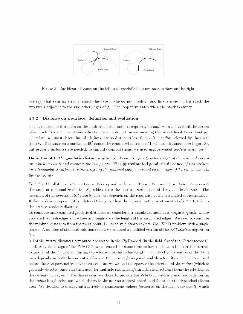
Figure 3: Euclidean distance on the left, and geodetic distance on a surface on the right.
one (fj) that satis�es error ", insert this face in the output mesh T , and �nally insert in the stack the
two pfe's adjacent to the two other edges of fj . The loop terminates when the stack is empty.
4.3.2 Distance on a surface: de�nition and evaluation
The evaluation of distances on the multiresolution mesh is required, because we want to limit the action
of each selective re�nement/simpli�cation to a mesh portion surrounding the user-de�ned focus point pf .
Therefore, we must determine which faces are at distances less than r (the radius selected by the user)
from pf . Distances on a surface in IR3 cannot be computed in terms of Euclidean distances (see Figure 3),
but geodetic distances are needed; to simplify computations, we used approximated geodetic distances:
De�nition 4.1 The geodetic distance of two points on a surface S is the length of the minimal curved
arc which lies on S and connects the two points. The approximated geodetic distance of two vertices
on a triangulated surface T is the length of the minimal path, composed by the edges of T , which connects
the two points.
To de�ne the distance between two vertices v1 and v2 in a multiresolution model, we take into account
the mesh at maximal resolution S0, which gives the best approximation of the geodetic distance. The
precision of the approximated geodetic distance depends on the regularity of the tessellated representation.
If the mesh is composed of equilateral triangles, then the approximation is at most 2=p3 �= 1:154 times
the precise geodetic distance.
To compute approximated geodetic distances we consider a triangulated mesh as a weighted graph, whose
arcs are the mesh edges and whose arc weights are the length of the associated edges. We need to compute
the minimal distances from the focus point, i.e. to solve a Shortest Path Tree (SPT) problem with a single
source. A number of standard solutions exist; we adopted a modi�ed version of the SPT S Heap algorithm
[15].
All of the vertex distances computed are stored in the HyT model (in the �eld dist of the Vertex records).
During the design of the Zeta GUI, we discussed for some time on how to show to the user the current
extension of the focus area, during the selection of the radius length. The e�ective extension of the focus
area depends on both the current radius and the current focus point, and therefore it can't be determined
before these to parameters have been set. But we wanted to separate the selection of the radius (which is
generally selected once and then used for multiple re�nement/simpli�cation actions) from the selection of
the current focus point. For this reason, we chose to provide the Zeta GUI with a visual feedback during
the radius length selection, which shows to the user an approximated (and focus-point independent) focus
area. We decided to display interactively a transparent sphere (centered on the last focus point), which
11
only shows the magnitude of the current radius and is not related to the actual geodetic distance.
4.3.3 The Selective Re�nement/Simpli�cation algorithm
The selective re�nement/simpli�cation algorithm locally modi�es the current mesh T , which can be either
a surface extracted at constant error from the HyT model, or the composition of n subsequent selective
re�nements.
Selective re�nement/simpli�cation parameters (set by the user) are:
� the current point of focus pf ;
� the radius r of the current selective update;
� the error function E : IR+ ! ["1; "2] which sets the error expected for each element fi of the mesh
in the focus region as a function of the distance between fi and the focus point pf ; it is de�ned in
the interval ["1; "2], with "1 the approximation error that must be veri�ed by faces at distance zero
from pf and "2 the one for faces at distance r.
A re�nement or a simpli�cation action is performed depending on the current selection for the error
function E domain: if "1 < "2 than the user requests a local re�nement (approximation must be higher in
the point of focus than in the focus region boundary), otherwise a local simpli�cation has to be executed.
Obviously, if the focus region is entirely at approximation " < "1, then no selective re�nement is applied.
In the current implementation, the user may interactively de�ne the current function E by editing its
graph in the Error Function section (bottom-right of the Zeta main window, see Figure 8).
Given a the current mesh T , the Selective Re�nement algorithm builds progressively a new mesh
subsection and updates T . Starting from the facet edge nearest to the focus point, it starts a topologic
expansion by following the adjacency links and choosing the next faces by taking into account the E
function and the distance from the focus point. The topological expansion is implemented by using a
priority queue, which encodes the facet-edges which have to be expanded, and it is limited by both the
radius set by the user and the need to maintain connectivity between the re�ned region and the mesh T
to be updated. At the end, the current variable resolution mesh is updated by removing the mesh section
which has been replaced by the re�ned one.
Speci�cally, the main steps of the Selective Re�nement algorithm are:
� select the pfe fe which is nearest to pf and satis�es the precision "1 required for the focus point
(FindFirstEdge function);
� initialize the priority queue by inserting in it both fe and its adjacent fe.fother;
� compute geodetic distances from pf (SPT S Heap function);
� initialize to null the overlapStack, i.e. the data structure that will hold all the facet-edges on the
border of the re�ned mesh section;
� main loop:
{ extract the next pfe fe from the priority queue;
12
b
fa
current topologicalexpansion border
fa
fb
f
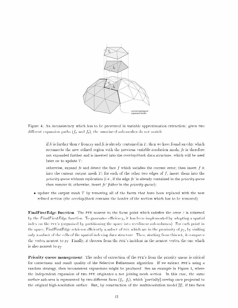
Figure 4: An inconsistency which has to be prevented in variable approximation extraction: given two
di�erent expansion paths (fa and fb), the associated sub-meshes do not match.
{ if fe is further than r from pf and fe is already contained in T , then we have found an edge which
reconnects the new re�ned region with the previous variable resolution mesh; fe is therefore
not expanded further and is inserted into the overlapStack data structure, which will be used
later on to update T ;
{ otherwise, expand fe and detect the face f which satis�es the current error; then insert f it
into the current output mesh T ; for each of the other two edges of f , insert them into the
priority queue without replication (i.e., if the edge fe' is already contained in the priority queue
then remove it; otherwise, insert fe'.fother in the priority queue);
� update the output mesh T by removing all of the facets that have been replaced with the new
re�ned section (the overlapStack contains the border of the section which has to be removed).
FindFirstEdge function. The pfe nearest to the focus point which satis�es the error " is returned
by the FindF irstEdge function. To guarantee e�ciency, it has been implemented by adopting a spatial
index on the pfe's (organised by partitioning the space into rectilinear sub-volumes). For each point in
the space, FindFirstEdge retrieves e�ciently a subset of pfe which are in the proximity of pf , by visiting
only a subset of the cells of the spatial indexing data structure. Then, starting from this set, it computes
the vertex nearest to pf . Finally, it chooses from the pfe's incident in the nearest vertex the one which
is also nearest to pf .
Priority queue management. The order of extraction of the pfe's from the priority queue is critical
for correctness and result quality of the Selective Re�nement algorithm. If we extract pfe's using a
random strategy, then inconsistent expansions might be produced. See an example in Figure 4, where
the independent expansion of two pfe originates a not joining mesh section. In this case, the same
surface sub-area is represented by two di�erent faces (fa, fb), which [partially] overlap once projected to
the original high-resolution surface. But, by construction of the multiresolution model [2], if two faces
13
represent (at least partially) the same original surface area, then their life intervals must be disjoint.
The case in Figure 4 can be prevented if we expand facet-edges by taking into account the global current
content of the priority queue. In particular, we impose the constraint that for all the facet-edges on the
priority queue the intersection of their life intervals has to be not empty. The inconsistency above is
therefore prevented, because as stated previously if two faces in the HyT model cover the same portion
of the original surface, then, by construction, their life intervals have to be disjoint. In other words,
facet-edge expansion and insertion on the priority queue have been designed so that in each instant an "
value exists such that " 2 LifeInterval(fei) for all facet-edges fe
iin the priority queue. This implies that
the expansion of each facet-edge is driven by the user-selected error function, but takes also into account
the status of the priority queue: a too much rapid decrease/increase of the error, such that the selected
error "i will be not contained in the current priority queue's life interval, is denied and clipped to the
nearest extreme of the current priority queue's life interval.
This condition imposes a limitation on the ability to reduce the error following the error function (let
us again assume we are executing a re�nement action). In the case of a facet-edge with several possible
adjacent faces, we may be limited in the choice of the next face by the current status of the priority
queue: the best �t face, according to the distance{based error function, may result in the choice of an
error value which is not contained in the current intersection of all life intervals currently stored in the
priority queue. Let us introduce some more terminology to clarify the approach: given a priority queue
Q and the set of life intervals of all the facet-edges ei stored in Q, the intersection of all the life intervals
is delimited by:
Q:"maxb
= maxe2Q
e:"b ; Q:"min
d= min
e2Q
e:"d :
Therefore, for each new expansion we need to test if the proper distance{based error is contained in the
priority queue current interval [Q:"maxb
; Q:"mind
). The priority queue has to be implemented at least as a
double heap, to hold e�ciently the ordering of both the extreme values of the life interval.
A crucial point of the algorithm is now how to select the next pfe to be popped from the priority
queue, and this choice has a strong impact on the quality of the variable resolution mesh extracted. As
stated above, to ensure the validity of the mesh extracted it is mandatory to search for a face at an error
included in the interval [Q:"maxb
; Q:"mind
). If we extract from Q adopting a naive selection criterion (e.g.
FIFO), then the [Q:"maxb
; Q:"mind
) interval may become very narrow (in many cases it is reduced to a
single value), thus preventing us from following the required error decrease/increase encoded by the E
function. To maintain this interval as wide as possible, we evaluated di�erent priority queue management
strategies:
� distance-based popping: we extract in order of distance (nearest �rst) from the focus point pf ; to
assure e�ciency, Q has to be implemented as a triple heap, to provide a further sorting based on
facet-edge distances;
� error-based popping: we extract the pfe whose error interval is origin of the bounds of the current
priority queue interval; a side-e�ect of extracting that pfe is to widen the current priority queue
life interval. If we are re�ning the mesh, i.e. extracting a sub-mesh with an error which increases as
we get far from pf , then we extract the facet-edge with "d = Q:"mind
; otherwise, if we are reducing
resolution we select and extract the facet-edge with "b = Q:"maxb
;
� composed distance-error based popping: we follow a distance-based approach until we can extract
facet-edges at the proper error; then, we use the error-based criterion until the current priority
14
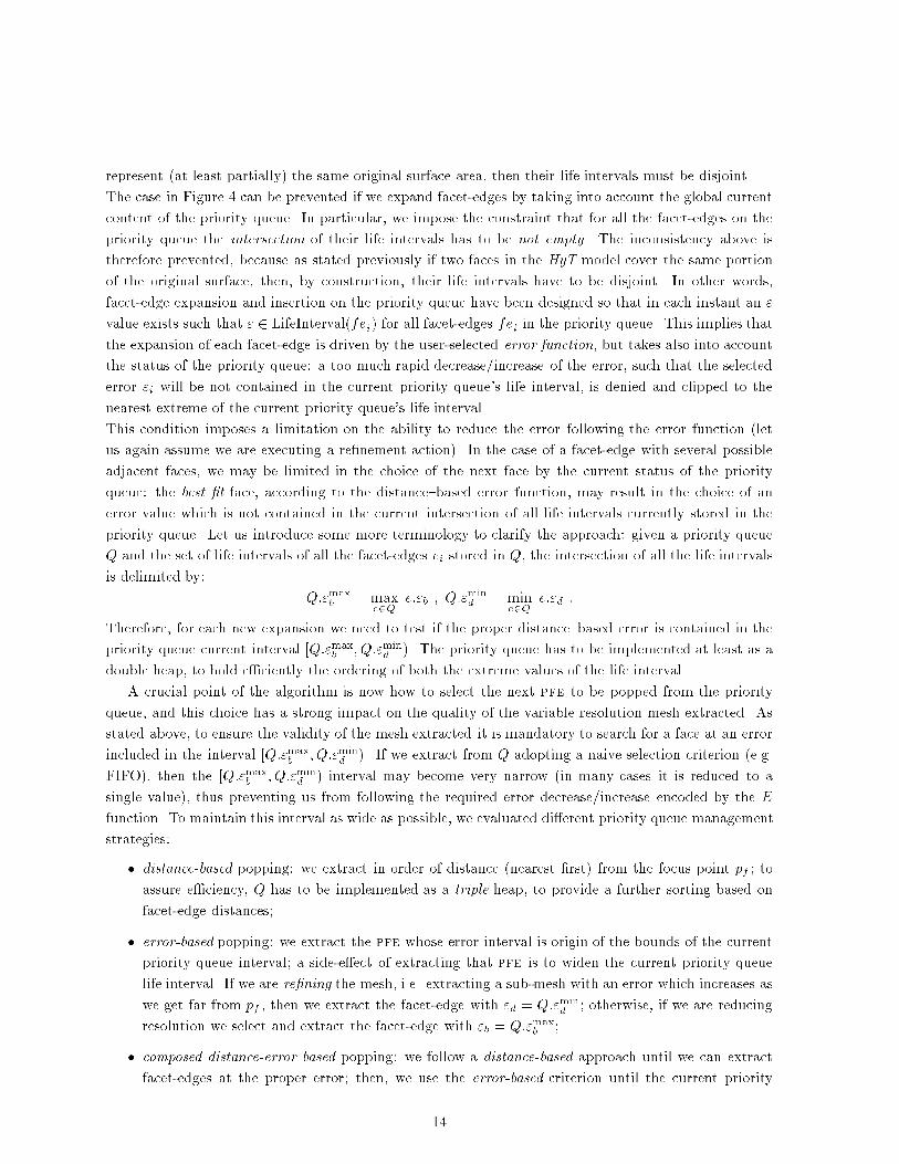
Procedure SelectiveRe�nement (HyT : MultiResScheme,
E: Function(d: Real ), radius: Real, fp: Point, Var T : Triangulation);
Var Q : TripleHeap;
overlapStack : Stack;
edge : PackedFacetEdge;
face : Face;
Begin
overlapStack := ;;
edge := FindFirstEdge(HyT , fp, E(0));
SPT S Heap Local(edge:vert, radius, HyT );
Q := fedgeg [ fedge:fotherg;
While Q 6= ; Do
PopEdge&ChooseFace(HyT , Q, T , radius, edge,
face, overlapStack);
If edge 6= ; AND face 6= ; Then
T := T [ ffaceg;
For i:=1 To 2 Do Begin
edge := edge.enext(face);
If edge 2 Q Then Q:= Q - fedgeg;
Else Q:= Q [ fedge:fotherg;
DeleteOverlap(overlapStack,T )
End;
Figure 5: Selective Re�nement pseudo code.
queue life interval has been su�ciently widened.
The previous strategies were evaluated on a number of datasets, and the composed distance-error
strategy gave the best performances, in terms of quality of the extracted mesh. The composed strategy
has been adopted in the Zeta prototype (see the pseudo code of Figure 6).
Facet-edge expansion and mesh update
For each facet-edge fe popped from the priority queue Q, if the distance of fe from pf is greater than the
radius r of the current selective update, and fe is already contained in the current mesh T , then we do not
proceed with the expansion of fe, and its adjacent facet-edge fe.fother is inserted into the overlapStack.
If, conversely, fe is farther than r but is not contained in T , we cannot stop the expansion (to prevent
cracks in the updated mesh T ), and thus proceed with the expansion of fe.
In canonical conditions, at the end of the topological expansions the boundary of the section of the
mesh T which has been re�ned is stored in the overlapStack. The DeleteOverlap() function removes
from T the redundant faces: it starts from the facet-edges contained in the overlapStack and removes
all of the faces which can be reached from these facet-edges and have a value of the �eld mark lower
than the current re�nement time (see Figure 7). The mark �eld of a Face record is a counter, whose
value is initialized with the \time" of the selective re�nement action that included such a face in mesh T .
15
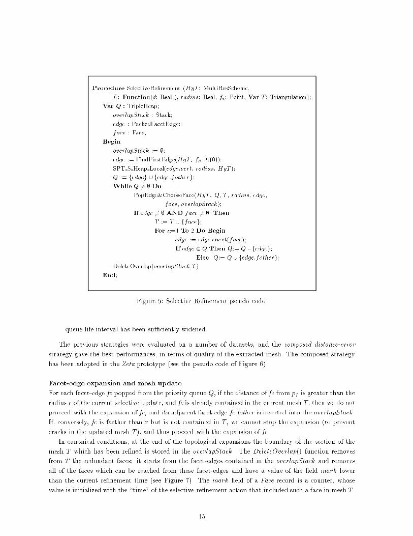
Procedure PopEdge&ChooseFace(HyT : MultiResScheme, Q: TripleHeap,
T : Triangulation, radius: Real, Var edge: PackedFacetEdge,
Var face: Face, Var overlapStack : Stack);
minErr;maxErr : Real;
Begin
edge := GetMinDistEdge(Q);
If edge 2 T And Dist(HyT ,edge) � radius
Then overlap := overlap [ fedge:fotherg;
edge := ;; face := ;;
Else � := E( Dist(HyT ,edge) );
minErr := GetMax"b(Q);
maxErr := GetMin"d(Q);
Case
� < minErr Then
edge := RemoveMinBirthEdge(Q);
face := FirstFace(edge)
� � maxErr Then
edge := RemoveMaxDeathEdge(Q);
face := LastFace(edge)
minErr � � < maxErr Then
edge := RemoveMinDistEdge(Q);
face := FindValidFace(edge,�)
End;
Figure 6: Selective Re�nement: selection and expansion of the next facet-edge from the priority queue.
Therefore, if a face f can be reached from the oriented boundary stored in overlapStack and it has been
inserted in T as part of a previous re�nement, then f is part of the replaced patch and can be removed
from T .
The di�erence between the focus area of the current selective re�nement/simpli�cation action and the
actual size of the updated mesh section is shown in Figure 11. The colored mesh section represents the
updated mesh region, and the color represents the geodetic distance from the current focus point. Faces
rendered in white are those which were produced with distance higher than the current radius (i.e. out
of the focus area), and which are needed to assure continuity of the variable resolution mesh.
5 Multiresolution Shape Editing
Simple shape editing features have been also included in the Zeta prototype, to show how mesh editing
might be performed in a consistent manner on the multiresolution model. The goal is obviously not to
support sophisticated functionalities (available in the shape editing framework), but to allow users to
perform small changes to the shape of the model, without requiring to traverse again the entire pipeline
(shape modeling, multiresolution construction, resolution modeling).
Shape editing actions are operated on the multiresolution scheme, and therefore shape changes are applied
to every resolution. A shape editing session is started by selecting the Edit Shape option of the Edit menu.
16
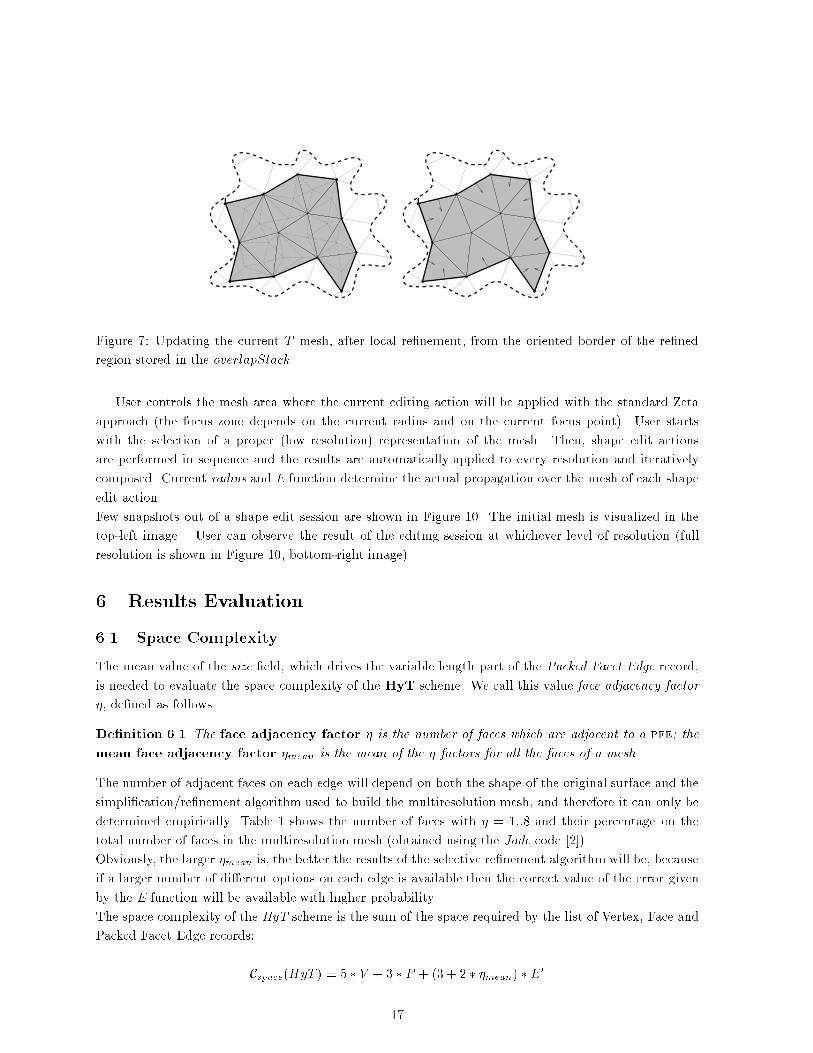
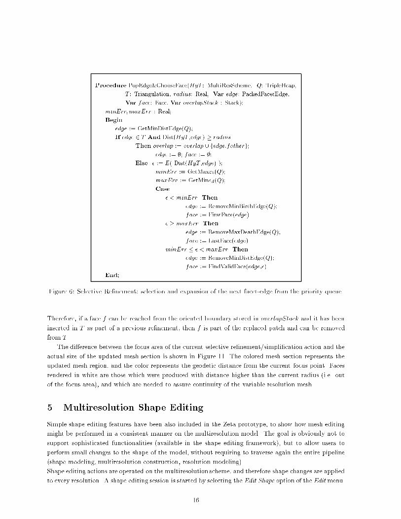
Figure 7: Updating the current T mesh, after local re�nement, from the oriented border of the re�ned
region stored in the overlapStack.
User controls the mesh area where the current editing action will be applied with the standard Zeta
approach (the focus zone depends on the current radius and on the current focus point). User starts
with the selection of a proper (low resolution) representation of the mesh. Then, shape edit actions
are performed in sequence and the results are automatically applied to every resolution and iteratively
composed. Current radius and E function determine the actual propagation over the mesh of each shape
edit action.
Few snapshots out of a shape edit session are shown in Figure 10. The initial mesh is visualized in the
top-left image. User can observe the result of the editing session at whichever level of resolution (full
resolution is shown in Figure 10, bottom-right image).
6 Results Evaluation
6.1 Space Complexity
The mean value of the size �eld, which drives the variable length part of the Packed Facet Edge record,
is needed to evaluate the space complexity of the HyT scheme. We call this value face adjacency factor
�, de�ned as follows.
De�nition 6.1 The face adjacency factor � is the number of faces which are adjacent to a pfe; the
mean face adjacency factor �mean is the mean of the � factors for all the faces of a mesh.
The number of adjacent faces on each edge will depend on both the shape of the original surface and the
simpli�cation/re�nement algorithm used to build the multiresolution mesh, and therefore it can only be
determined empirically. Table 1 shows the number of faces with � = 1::8 and their percentage on the
total number of faces in the multiresolution mesh (obtained using the Jade code [2]).
Obviously, the larger �mean is, the better the results of the selective re�nement algorithm will be, because
if a larger number of di�erent options on each edge is available then the correct value of the error given
by the E function will be available with higher probability.
The space complexity of the HyT scheme is the sum of the space required by the list of Vertex, Face and
Packed Facet Edge records:
Cspace(HyT ) = 5 � V + 3 � F + (3 + 2 � �mean) �E0
17
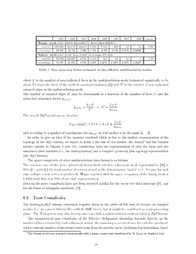
�=1 �=2 �=3 �=4 �=5 �=6 �=7 �=8 �mean
Bunny mesh (vert.:34,834 faces:189,351 facet-edges:568,053 )
number 241,066 99,139 28,821 7,529 1,821 401 67 14 1.54
percentage 63.6% 26.1% 7.6% 1.9% 0.4% 0.1% 0.01% 0.003%
Sphere mesh (vert.:6,322 faces:33,801 facet-edges:101,403)
number 43,788 18,427 4,744 1,114 322 63 11 1 1.48
percentage 63.9% 26.9% 6.9% 1.6% 0.47% 0.09% 0.01% 0.001%
Table 1: Face adjacency factor evaluated on two di�erent multiresolution meshes.
where F is the number of non replicated faces in the multiresolution mesh (estimated empirically to be
about 2.5 times the faces of the mesh at maximal resolution [2]) and E0 is the number of non replicated
oriented edges in the multiresolution mesh.
The number of oriented edges E0 may be determined as a function of the number of faces F and the
mean face adjacency factor �mean:
�mean =3 � FE0
! E0 =3 � F�mean
The overall HyT model size is therefore:
Cspace(HyT ) = 5 � V + 9 �F +9 � F�mean
and according to a number of experiments the �mean on real meshes is in the range [1 .. 2].
In order to give an idea of the memory overhead which is due to the explicit representation of the
topology in the HyT scheme, we report in Table 2 the size of two meshes, the Bunny3 and the Fandisk
meshes (shown in Figures 9 and 12), considering both the representation of only the faces and the
associated error intervals (i.e., the history format) and a complete geometry plus topology representation
(the HyT format).
The space complexity of other multiresolution data format is as follows.
The run-time size of the (non optimized) hierarchical selective re�nement mesh representation [20] is
224� jV̂ j, with jV̂ j the total number of vertices stored in the data structure (and V̂ > V , because for each
edge collapse a new vertex is produced). Hoppe reported that the space occupancy of the bunny mesh is
7.8MB (and thus it is 72% of our HyT representation).
Data on the space complexity have not been reported neither for the merge tree data structure [31], nor
for the forest of triangular quadtrees [32].
6.2 Time Complexity
The history to HyT scheme conversion requires times in the order of few tens of seconds on complex
meshes (i.e. to convert history �les with �= 100K faces), but it might be considered as a pre-processing
phase. The Zeta system may also directly save onto disk a multiresolution mesh encoded in HyT format.
The asymptotical time complexity of the Selective Re�nement algorithm depends directly on the
number of faces returned by each re�nement action: the main loop is executed once for each face produced,
with a constant number of insertions/extractions from the priority queue (performed in logarithmic time).
3The Bunny model was acquired automatically with a range scanner and distributed by M. Levoy at Stanford Univ.
18
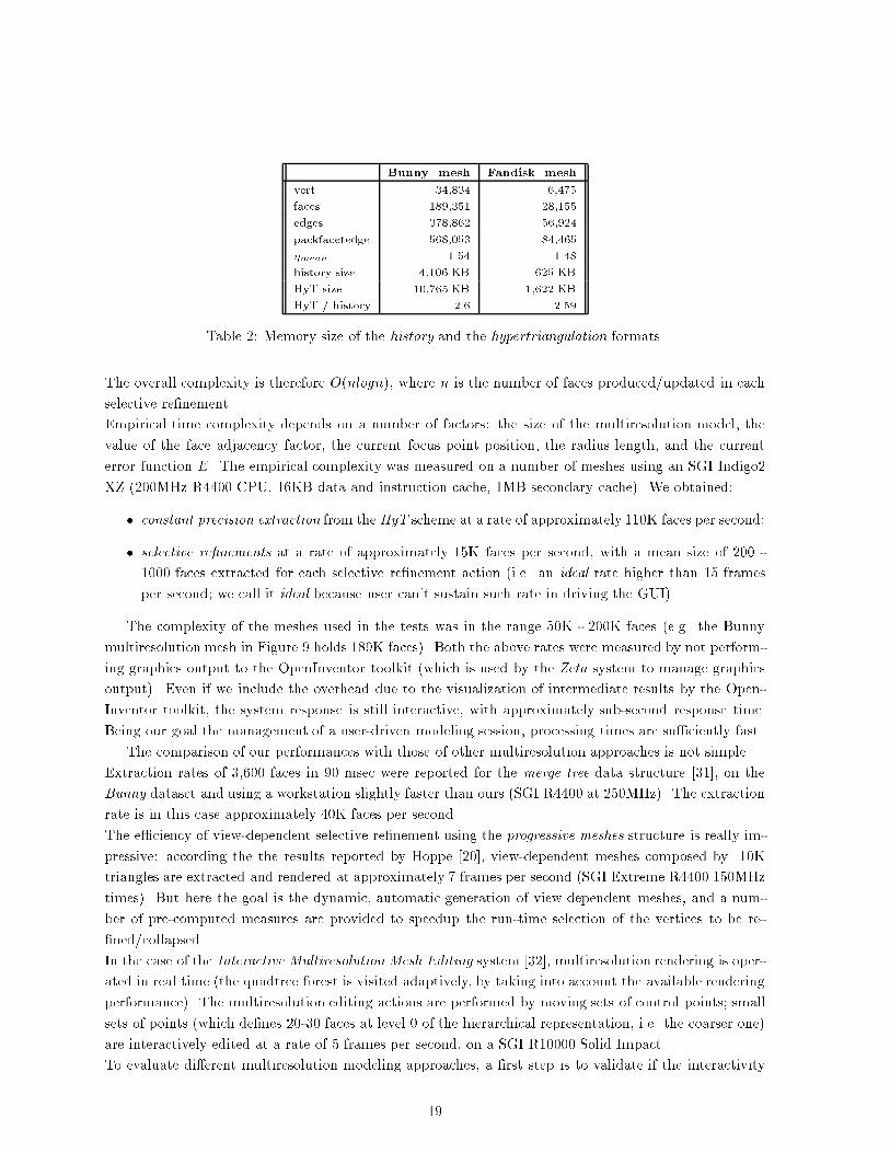
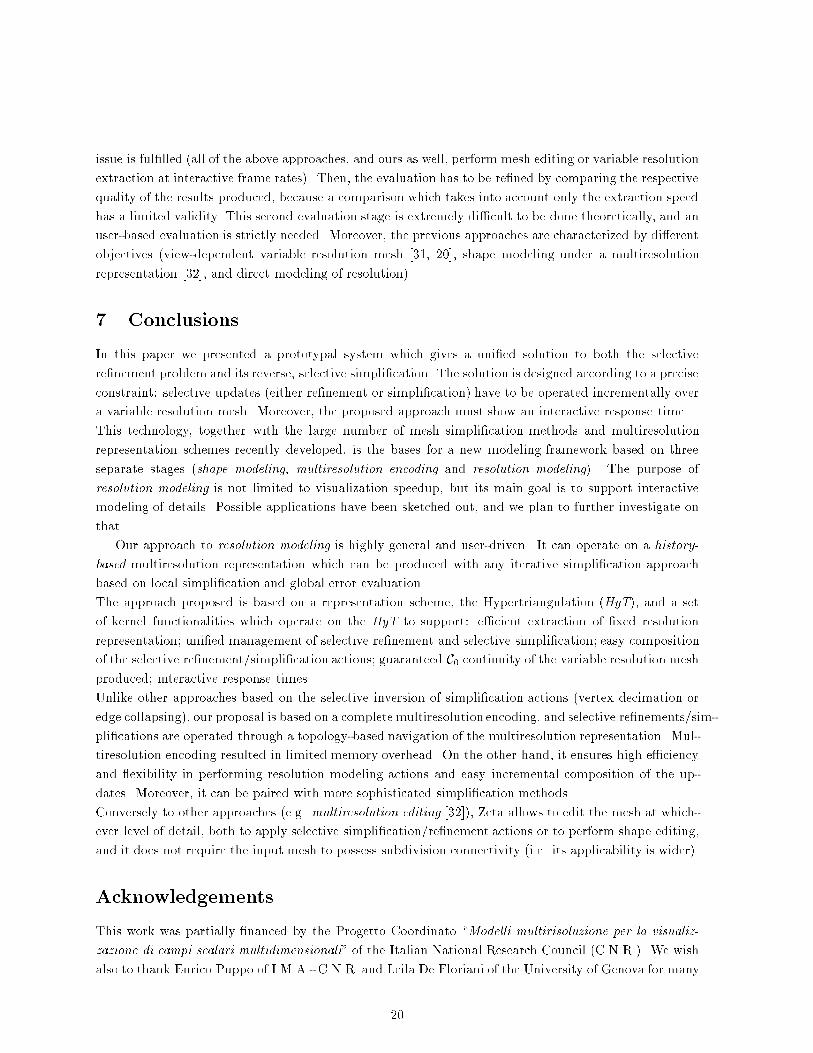
Bunny mesh Fandisk mesh
vert. 34,834 6,475
faces 189,351 28,155
edges 378,862 56,924
packfacetedge 568,053 84,465
�mean 1.54 1.48
history size 4,106 KB 625 KB
HyT size 10,765 KB 1,622 KB
HyT / history 2.6 2.59
Table 2: Memory size of the history and the hypertriangulation formats.
The overall complexity is therefore O(nlogn), where n is the number of faces produced/updated in each
selective re�nement.
Empirical time complexity depends on a number of factors: the size of the multiresolution model, the
value of the face adjacency factor, the current focus point position, the radius length, and the current
error function E. The empirical complexity was measured on a number of meshes using an SGI Indigo2
XZ (200MHz R4400 CPU, 16KB data and instruction cache, 1MB secondary cache). We obtained:
� constant precision extraction from the HyT scheme at a rate of approximately 110K faces per second;
� selective re�nements at a rate of approximately 15K faces per second, with a mean size of 200 -
1000 faces extracted for each selective re�nement action (i.e. an ideal rate higher than 15 frames
per second; we call it ideal because user can't sustain such rate in driving the GUI).
The complexity of the meshes used in the tests was in the range 50K - 200K faces (e.g. the Bunny
multiresolution mesh in Figure 9 holds 189K faces). Both the above rates were measured by not perform-
ing graphics output to the OpenInventor toolkit (which is used by the Zeta system to manage graphics
output). Even if we include the overhead due to the visualization of intermediate results by the Open-
Inventor toolkit, the system response is still interactive, with approximately sub-second response time.
Being our goal the management of a user-driven modeling session, processing times are su�ciently fast.
The comparison of our performances with those of other multiresolution approaches is not simple.
Extraction rates of 3,600 faces in 90 msec were reported for the merge tree data structure [31], on the
Bunny dataset and using a workstation slightly faster than ours (SGI R4400 at 250MHz). The extraction
rate is in this case approximately 40K faces per second.
The e�ciency of view-dependent selective re�nement using the progressive meshes structure is really im-
pressive: according the the results reported by Hoppe [20], view-dependent meshes composed by 10K
triangles are extracted and rendered at approximately 7 frames per second (SGI Extreme R4400 150MHz
times). But here the goal is the dynamic, automatic generation of view dependent meshes, and a num-
ber of pre-computed measures are provided to speedup the run-time selection of the vertices to be re-
�ned/collapsed.
In the case of the Interactive Multiresolution Mesh Editing system [32], multiresolution rendering is oper-
ated in real time (the quadtree forest is visited adaptively, by taking into account the available rendering
performance). The multiresolution editing actions are performed by moving sets of control points; small
sets of points (which de�nes 20-30 faces at level 0 of the hierarchical representation, i.e. the coarser one)
are interactively edited at a rate of 5 frames per second, on a SGI R10000 Solid Impact.
To evaluate di�erent multiresolution modeling approaches, a �rst step is to validate if the interactivity
19
issue is ful�lled (all of the above approaches, and ours as well, perform mesh editing or variable resolution
extraction at interactive frame rates). Then, the evaluation has to be re�ned by comparing the respective
quality of the results produced, because a comparison which takes into account only the extraction speed
has a limited validity. This second evaluation stage is extremely di�cult to be done theoretically, and an
user-based evaluation is strictly needed. Moreover, the previous approaches are characterized by di�erent
objectives (view-dependent variable resolution mesh [31, 20], shape modeling under a multiresolution
representation [32], and direct modeling of resolution).
7 Conclusions
In this paper we presented a prototypal system which gives a uni�ed solution to both the selective
re�nement problem and its reverse, selective simpli�cation. The solution is designed according to a precise
constraint: selective updates (either re�nement or simpli�cation) have to be operated incrementally over
a variable resolution mesh. Moreover, the proposed approach must show an interactive response time.
This technology, together with the large number of mesh simpli�cation methods and multiresolution
representation schemes recently developed, is the bases for a new modeling framework based on three
separate stages (shape modeling, multiresolution encoding and resolution modeling). The purpose of
resolution modeling is not limited to visualization speedup, but its main goal is to support interactive
modeling of details. Possible applications have been sketched out, and we plan to further investigate on
that.
Our approach to resolution modeling is highly general and user-driven. It can operate on a history-
based multiresolution representation which can be produced with any iterative simpli�cation approach
based on local simpli�cation and global error evaluation.
The approach proposed is based on a representation scheme, the Hypertriangulation (HyT), and a set
of kernel functionalities which operate on the HyT to support: e�cient extraction of �xed resolution
representation; uni�ed management of selective re�nement and selective simpli�cation; easy composition
of the selective re�nement/simpli�cation actions; guaranteed C0 continuity of the variable resolution mesh
produced; interactive response times.
Unlike other approaches based on the selective inversion of simpli�cation actions (vertex decimation or
edge collapsing), our proposal is based on a complete multiresolution encoding, and selective re�nements/sim-
pli�cations are operated through a topology-based navigation of the multiresolution representation. Mul-
tiresolution encoding resulted in limited memory overhead. On the other hand, it ensures high e�ciency
and exibility in performing resolution modeling actions and easy incremental composition of the up-
dates. Moreover, it can be paired with more sophisticated simpli�cation methods.
Conversely to other approaches (e.g. multiresolution editing [32]), Zeta allows to edit the mesh at which-
ever level of detail, both to apply selective simpli�cation/re�nement actions or to perform shape editing,
and it does not require the input mesh to possess subdivision connectivity (i.e. its applicability is wider).
Acknowledgements
This work was partially �nanced by the Progetto Coordinato \Modelli multirisoluzione per la visualiz-
zazione di campi scalari multidimensionali" of the Italian National Research Council (C.N.R.). We wish
also to thank Enrico Puppo of I.M.A.- C.N.R. and Leila De Floriani of the University of Genova for many
20
useful discussions and comments.
References
[1] A. Certain, J. Popovic, T. DeRose, T. Duchamp, D. Salesin, and W. Stuetzle. Interactive multires-
olution surface viewing. In Comp. Graph. Proc., Annual Conf. Series (Siggraph '96), ACM Press,
pages 91{98, Aug. 6-8 1996.
[2] A. Ciampalini, P. Cignoni, C. Montani, and R. Scopigno. Multiresolution decimation based on global
error. The Visual Computer, 13(5):228{246, June 1997.
[3] P. Cignoni, C. Montani, E. Puppo, and R. Scopigno. Multiresolution modeling and visualization of
volume data. IEEE Trans. on Visualization and Comp. Graph., 3(4):352{369, 1997.
[4] P. Cignoni, E. Puppo, and R. Scopigno. Representation and visualization of terrain surfaces at
variable resolution. The Visual Computer, 13(5):199{217, 1997.
[5] J. H. Clark. Hierarchical geometric models for visible surface algorithms. Comm. of the ACM,
19(10):547{554, Oct. 1976.
[6] J. Cohen, A. Varshney, D. Manocha, G. Turk, H. Weber, P. Agarwal, F. Brooks, and W. Wright.
Simpli�cation envelopes. In Computer Graphics Proc., Annual Conf. Series (Siggraph '96), ACM
Press, pages 119{128, Aug. 6-8 1996.
[7] M. de Berg and K. Dobrindt. On levels of detail in terrains. In Proceedings 11th ACM Symposium
on Computational Geometry, pages C26{C27, Vancouver (Canada), 1995. ACM Press.
[8] L. De Floriani, P. Marzano, and E. Puppo. Multiresolution models for topographic surface descrip-
tion. The Visual Computer, 12(7):317{345, 1996.
[9] D.P. Dobkin and M.J. Laszlo. Primitives for the manipulation of three{dimensional subdivisions.
Algorithmica, 4:3{32, 1989.
[10] M.A. Duchaineau, M. Wolinsky, D.E. Sigeti, M.C. Miller, C. Aldrich, and M.B. Mineev-Weinstein.
ROAMing terrain: Real-time optimally adapting meshes. In IEEE Visualization '97, October 1997.
[11] M. Eck, T. De Rose, T. Duchamp, H. Hoppe, M. Lounsbery, and W. Stuetzle. Multiresolution
analysis of arbitrary meshes. In Computer Graphics Proc., Annual Conf. Series (Siggraph '95),
ACM Press, pages 173{181, Aug. 6-12 1995.
[12] D.R. Forsey and R.H. Bartels. Hierarchical b-spline re�nement. Computer Graphics (SIGGRAPH
'88 Proceedings), 22(4):205{212, August 1988.
[13] R.J. Fowler and J.J. Little. Automatic extraction of irregular network digital terrain models. ACM
Computer Graphics (Siggraph '79 Proc.), 13(3):199{207, Aug. 1979.
[14] T.A. Funkhouser and C.H. Sequin. Adaptive display algorithm for interactive frame rates during vi-
sualization of complex environment. In Computer Graphics Proc., Annual Conf. Series (SIGGRAPH
93), pages 247{254. ACM Press, 1993.
21
[15] G. Gallo and S. Pallottino. Shortest path algorithms. Annals of Operations Research, 13:3{79, 1988.
[16] M. Garland and P.S. Heckbert. Surface simpli�cation using quadric error metrics. In Comp. Graph.
Proc., Annual Conf. Series (Siggraph '97), ACM Press, pages 209{216, 1997.
[17] M.H. Gross, O.G. Staadt, and R. Gatti. E�cient triangular surface approximations using wavelets
and quadtree data structures. IEEE Trans. on Visual. and Comp. Graph., 2(2):130{144, June 1996.
[18] P. Heckbert and M. Garland. Multiresolution Modeling for Fast Rendering. In Graphics Interface
'94 Proceedings, pages 43{50, 1994.
[19] H. Hoppe. Progressive meshes. In ACM Computer Graphics Proc., Annual Conference Series,
(Siggraph '96), pages 99{108, 1996.
[20] Hugues Hoppe. View-dependent re�nement of progressive meshes. In ACM Computer Graphics
Proc., Annual Conference Series, (Siggraph '97), 1997. 189-198.
[21] Hugues Hoppe, Tony DeRose, Tom Duchamp, John McDonald, and Werner Stuetzle. Mesh op-
timization. In ACM Computer Graphics Proc., Annual Conference Series, (Siggraph '93), pages
19{26, 1993.
[22] R. Klein, G. Liebich, and W. Stra�er. Mesh reduction with error control. In R. Yagel and G. Nielson,
editors, Proceedings of Visualization `96, pages 311{318, 1996.
[23] P. Lindstrom, D. Koller, W. Ribarsky, L.F. Hodges, N. Faust, and G.A. Turner. Real-time, continu-
ous level of detail rendering of height �elds. In Comp. Graph. Proc., Annual Conf. Series (Siggraph
'96), ACM Press, pages 109{118, New Orleans, LA, USA, Aug. 6-8 1996.
[24] E. Puppo and R. Scopigno. Simpli�cation, LOD, and Multiresolution - Principles and Applications.
In EUROGRAPHICS'97 Tutorial Notes (ISSN 1017-4656). Eurographics Association, Aire-la-Ville
(CH), 1997 (PS97 TN4).
[25] R. Ronfard and J. Rossignac. Full-range approximation of triangulated polyhedra. Computer Graph-
ics Forum (Eurographics'96 Proc.), 15(3):67{76, 1996.
[26] J. Rossignac and P. Borrel. Multi-resolution 3D approximation for rendering complex scenes. In
B. Falcidieno and T.L. Kunii, editors, Geometric Modeling in Computer Graphics, pages 455{465.
Springer Verlag, 1993.
[27] Lori Scarlatos and Theo Pavlidis. Hierarchical triangulation using cartographics coherence. CVGIP:
Graphical Models and Image Processing, 54(2):147{161, March 1992.
[28] William J. Schroeder, Jonathan A. Zarge, and William E. Lorensen. Decimation of triangle meshes.
In Edwin E. Catmull, editor, ACM Computer Graphics (SIGGRAPH '92 Proceedings), volume 26,
pages 65{70, July 1992.
[29] Greg Turk. Re-tiling polygonal surfaces. In Edwin E. Catmull, editor, ACM Computer Graphics
(SIGGRAPH '92 Proceedings), volume 26, pages 55{64, July 1992.
22

[30] J. Wilhelms and A. van Gelder. Multi-dimensional Trees for Controlled Volume Rendering and
Compression. In Proceedings of 1994 Symposium on Volume Visualization, pages 27{34. ACM Press,
October 17-18 1994.
[31] J.C. Xia, J. El-Sana, and A. Varshney. Adaptive real-time level-of-detail-based rendering for polyg-
onal models. IEEE Trans. on Visualization and Computer Graphics, 3(2):171{183, 1997.
[32] D. Zorin, P. Schr�oder, and W. Sweldens. Interactive multiresolution mesh editing. In Comp. Graph.
Proc., Annual Conf. Series (Siggraph '97), ACM Press, 1997. 259-268.
23
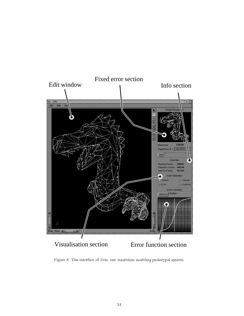
Edit windowFixed error section
Info section
Visualisation section Error function section
Figure 8: The interface of Zeta, our resolution modeling prototypal system.
24
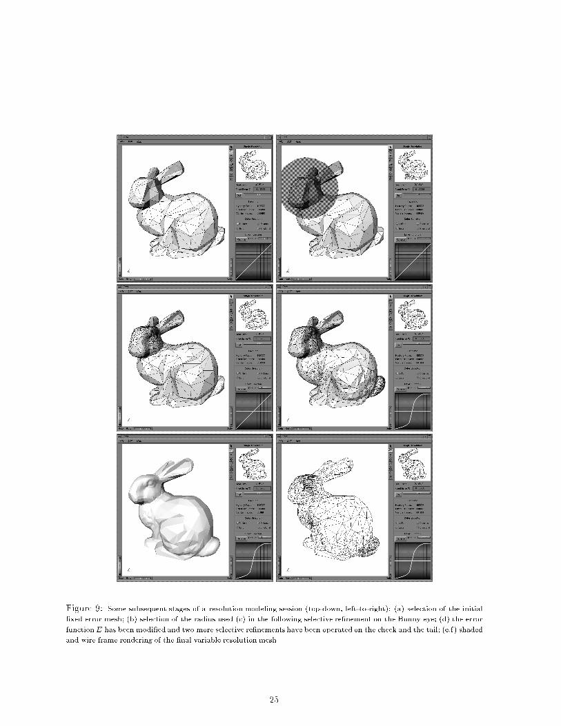
Figure 9: Some subsequent stages of a resolution modeling session (top-down, left-to-right): (a) selection of the initial
�xed error mesh; (b) selection of the radius used (c) in the following selective re�nement on the Bunny eye; (d) the error
function E has been modi�ed and two more selective re�nements have been operated on the cheek and the tail; (e,f) shaded
and wire frame rendering of the �nal variable resolution mesh.
25
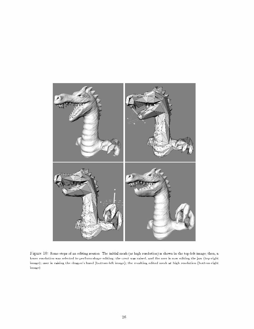
Figure 10: Some steps of an editing session. The initial mesh (at high resolution) is shown in the top-left image; then, a
lower resolution was selected to perform shape editing: the crest was raised, and the user is now editing the jaw (top-right
image); user is raising the dragon's hand (bottom-left image); the resulting edited mesh at high resolution (bottom-right
image).
26
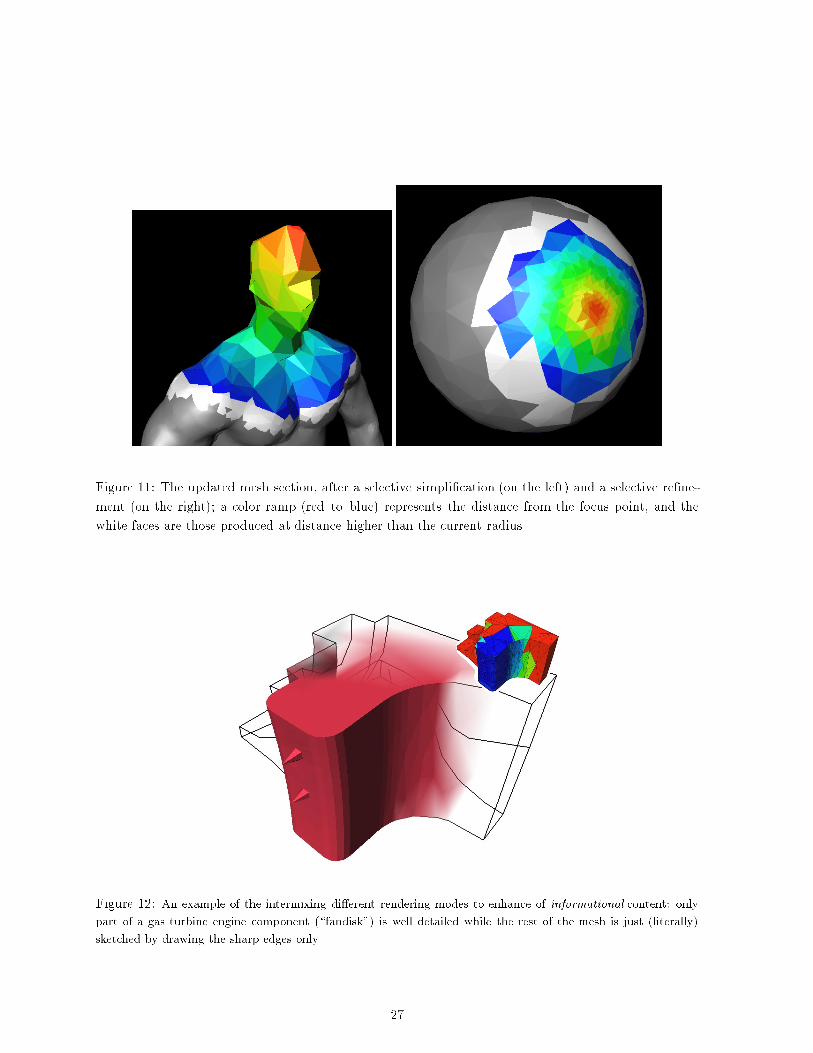
Figure 11: The updated mesh section, after a selective simpli�cation (on the left) and a selective re�ne-
ment (on the right); a color ramp (red{to{blue) represents the distance from the focus point, and the
white faces are those produced at distance higher than the current radius.
Figure 12: An example of the intermixing di�erent rendering modes to enhance of informational content: only
part of a gas turbine engine component (\fandisk") is well detailed while the rest of the mesh is just (literally)
sketched by drawing the sharp edges only.
27
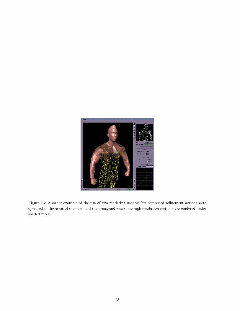
Figure 13: Another example of the use of two rendering modes; few composed re�nement actions were
operated in the areas of the head and the arms, and also these high resolution sections are rendered under
shaded mode.
28