Embed Size (px)
Citation preview

A RESISTANCE BASED
STRUCTURAL HEALTH MONITORING SYSTEM
FOR
COMPOSITE STRUCTURE APPLICATIONS
A Thesis
presented to
the Faculty of California Polytechnic State University,
San Luis Obispo, CA
In Partial Fulfillment
of the Requirements for the Degree of
Master of Science in Aerospace Engineering
By
Dennis N. Boettcher
August 2012

© 2012
Dennis N. Boettcher
All Rights Reserved

iii
COMMITTEE MEMBERSHIP
TITLE: A Resistance Based
Structural Health Monitoring System
for
Composite Structure Applications
AUTHOR: Dennis N. Boettcher
DATE
SUBMITTED: June 30, 2012
Committee Chair: Dr. Faysal A. Kolkailah, Ph.D., P.E.
Committee Member: Dr. Eltahry Elghandour, Ph. D.
Committee Member: Dr. Susan Opava, Ph. D.
Committee Member: Dr. Matthew Moelter, Ph. D.

iv
ABSTRACT
A Resistance Based Structural Health Monitoring System for Composite Structure Applications
by
Dennis N. Boettcher
This research effort explored the possibility of using interwoven conductive and
nonconductive fibers in a composite laminate for structural health monitoring (SHM).
Traditional SHM systems utilize fiber optics, piezoelectrics, or detect defects by nondestructive
test methods by use of sonar graphs or x-rays. However, these approaches are often expensive,
time consuming and complicated.
The primary objective of this research was to apply a resistance based method of
structural health monitoring to a composite structure to determine structural integrity and
presence of defects.
The conductive properties of fiber such as carbon, copper, or constantan - a copper-nickel
alloy - can be utilized as sensors within the structure. This allows the structure to provide
feedback via electrical signals to a user which are essential for evaluating the health of the
structure. In this research, the conductive fiber was made from constantan wire which was
embedded within a composite laminate; whereas prepreg fiberglass, a nonconductive material,
serves as the main structural element of the laminate. A composite laminate was constructed
from four layers of TenCate 7781 “E” fiberglass and BT250E-1 resin prepreg. Integrating the
constantan within the composite laminate provides a sensory element which supplies
measurements of structural behavior. Thus, with fiberglass, epoxy, and a constantan conductive
element, a three-part composite laminate is developed.
Test specimens used in this research were fabricated using a composite air press with the
recommended manufacturer cure cycle. A TenCate BT250E-1 Resin System and 7781 "E"
impregnated glass-fiber/epoxy weave was used. A constantan wire of 0.01” gauge diameter was

v
integrated into the composite structure. The composite laminate specimen with the integrated
SHM system was tested under tensile and flexural loads employing test standards specified by
ASTM D3039 and D7264, respectively. These test methods were modified to determine the
behavior of the laminate in the elastic range only. A tension and flexural delamination test case
was also developed to investigate the sensitivity of the SHM system to inherent defects.
Moreover, material characteristic tests were completed to validate manufacturer provided
material characteristics. The specimens were tested while varying the constantan configurations,
such as the sensor length and orientation. A variety of techniques to integrate the sensor were
also investigated. Two different measurement methods were used to determine strain. Strain
measurements were made with Instron Bluehill 2 software and correlated to strain obtained by
the structural health monitoring system with the use of a data acquisition code written to interact
with a micro-ohm-meter.
The experimental results showed good agreement between measurements made by the
two different methods of measurement. Observations discovered that varying the length of the
sensor element improved sensitivity, but resulted in different prediction models when compared
to cases with less sensor length. The predictions are based on the gauge factor, which was
determined for the each test case. This value provides the essential relationship between
resistance and strain. Experiments proved that the measured gauge factor depended greatly on
the sensor length and orientation. The correlation was of sufficient accuracy to predict strain
values in a composite laminate without the use of any added tools or equipment besides the ohm-
meter.
Analytical solutions to the loading cases were developed to validate results obtained
during experiments. The solutions were in good agreement with the experimental results.

vi
ACKNOWLEDGEMENTS Firstly, thank you to Dr. Faysal Kolkailah. His wisdom has been extremely helpful in
aspects related to this project as well as non-technical issues. His advice and inspiration have
helped guide me in many aspects related to engineering and life. I am sincerely grateful for the
faculty understanding, support and dedicated assistance to my project efforts, education and non-
scholastic development.
Secondly, I would like to thank Dr. Eltahry Elghandour who has been essential to the
success of this research effort. I am very grateful to have been provided with the opportunity to
work with him on this project and many more. His guidance in the lab provided insightful
solutions to the many questions posed during the project effort. Additionally his experience
proved immensely valuable during experimental validation by providing direction in efforts
which may otherwise have been time consuming to explore.
Thank you, Gabe Sanchez and Kodi Rider for being great research associates. The help I
received in the lab is not without gratitude. And thank you to all other students and SAMPE Club
members who have accompanied me on this journey. Jay Lopez, Cameron Chan, Albert Liu, Abe
Shabbar, and Vanessa Wood who made lab time much more enjoyable.
Also many thanks to Kendall Oblak of TenCate for donating necessary materials for this
project. Also to Dr. Moelter for making test equipment available and offering guidance on test
software. Thank you to Dr. Opava for taking the time to review the work.
I am also grateful for my family and friends. This opportunity would not be possible
without them. Thanks to my mother and father for always believing in and supporting me even
with opposed opinions. Thank you to my aunts, uncles and grandparents for ensuring I am well
fed and never without entertainment. Thank you to my roommates and peers this job would have
been difficult without the merriment and distractions.

vii
TABLE OF CONTENTS
LIST OF TABLES .......................................................................................................................... x
LIST OF FIGURES ....................................................................................................................... xi
LIST OF EQUATIONS ............................................................................................................... xiv
CHAPTER 1. INTRODUCTION ................................................................................................... 1
1.1 COMPOSITE MATERIALS ........................................................................................... 1
1.1.1 Different forms of composites ........................................................................................ 2
1.1.2 Composite material advantages and disadvantages ........................................................ 4
1.1.3 Fibrous Composite Weave Varieties .............................................................................. 5
1.1.4 Manufacturing processes ................................................................................................ 6
1.2 STRUCTURAL HEALTH MONITORING SYSTEMS ................................................. 9
1.2.1 Fiber Bragg ................................................................................................................... 10
1.2.2 Piezoelectric .................................................................................................................. 10
1.2.3 Resistance & Strain Based ............................................................................................ 11
1.3 ELECTROTEXTILES ................................................................................................... 11
1.4 NONDESTRUCTIVE TEST METHODS ..................................................................... 13
1.4.1 Liquid Penetrant ........................................................................................................... 14
1.4.2 Magnetic Particle .......................................................................................................... 14
1.4.3 Ultrasonic...................................................................................................................... 15
1.4.4 Radiography.................................................................................................................. 15
1.4.5 Thermography .............................................................................................................. 16
1.4.6 Nondestructive Test Methods Summary ...................................................................... 16
1.5 LITERATURE REVIEW ............................................................................................... 17
1.6 SCOPE OF WORK ........................................................................................................ 19
CHAPTER 2. THEORY OF SYSTEM ........................................................................................ 21
2.1 SYSTEM ARCHITECTURE ......................................................................................... 21
2.2 STRAIN GAUGE THEORY ......................................................................................... 22
2.3 EXPERIMENTAL TESTING METHODS ................................................................... 25
2.4 MEASUREMENT DEVICES ....................................................................................... 26

viii
2.5 SYSTEM DESIGN ........................................................................................................ 27
CHAPTER 3. MANUFACTURING PROCESS .......................................................................... 30
3.1 COMPOSITE LAMINATE PLATE PREPARATIONS ............................................... 30
3.1.1 Material Characteristics ................................................................................................ 30
3.1.2 Laminate Preparation Process ...................................................................................... 33
3.1.3 Delaminated Specimen Preparation Process ................................................................ 34
3.2 CONDUCTIVE SENSOR PREPARATION ................................................................. 35
3.2.1 Material Characteristics ................................................................................................ 35
3.2.2 Full Length Linear Sensor ............................................................................................ 36
3.2.3 Threaded Through Linear Sensor ................................................................................. 38
3.2.4 Threaded Through Delaminated Linear Sensor ............................................................ 40
3.2.5 Threaded Through Parabolic Sensor ............................................................................ 40
3.2.6 Threaded Angled Linear Sensor ................................................................................... 41
3.2.7 Linear Perpendicular Sensor ......................................................................................... 42
3.2.8 Full Length Carbon Tow Sensor .................................................................................. 43
3.2.9 Threaded Through Linear Sensor for Fracture ............................................................. 44
3.2.10 Threaded Linear Sensor for Flexural .......................................................................... 45
3.2.11 Delaminated Threaded Linear Sensor for Flexural .................................................... 47
3.3 SPECIMEN PREPARATION ....................................................................................... 48
3.3.1 Cure Process ................................................................................................................. 48
3.3.2 Specimen Refinement ................................................................................................... 48
CHAPTER 4. EXPERIMENTAL ANALYSIS ............................................................................ 50
4.1 DETERMINATION OF MATERIAL PROPERTIES .................................................. 50
4.1.1 Poisson’s Ratio ............................................................................................................. 50
4.1.2 Weight Fraction ............................................................................................................ 58
4.1.3 Elastic Modulus ............................................................................................................ 61
4.1.4 Gauge Factor................................................................................................................. 63
4.2 TEST DEVICES ............................................................................................................ 68
4.2.1 Strain -Stress Test and Measurement Device ............................................................... 68
4.2.2 Resistance Measurement Device .................................................................................. 69
4.3 TEST SETUP ................................................................................................................. 73

ix
4.3.1 Tensile Testing Standards ............................................................................................. 73
4.3.2 Flexural Testing Standards ........................................................................................... 74
4.4 EXPERIMENTAL RESULTS ....................................................................................... 75
4.4.1 Threaded Through Linear Sensor ................................................................................. 75
4.4.2 Threaded Through Delaminated Sensor ....................................................................... 79
4.4.3 Threaded Through Parabolic Sensor ............................................................................ 81
4.4.4 Threaded Angled Linear Sensor ................................................................................... 84
4.4.5 Linear Perpendicular Sensor ......................................................................................... 87
4.4.6 Full Length Carbon Tow Sensor .................................................................................. 89
4.4.7 Threaded Through Linear Sensor for Fracture ............................................................. 93
4.4.8 Linear Threaded Through Sensor for Flexural ............................................................. 95
4.4.9 Delaminated Linear Threaded Through Sensor for Flexural ...................................... 100
4.5 SUMMARY OF EXPERIMENTS............................................................................... 106
CHAPTER 5. THEORETICAL ANALYSIS ............................................................................. 109
5.1 STRAIN PREDICTION ............................................................................................... 109
5.2 RESISTANCE PREDICTION ..................................................................................... 111
CHAPTER 6. CONCLUSION AND RECOMMENDATIONS ................................................ 114
6.1 FUTURE WORK AND IMPROVEMENTS ............................................................... 115
REFERENCES ........................................................................................................................... 117
APPENDIX ................................................................................................................................. 120

x
LIST OF TABLES Table 1. Composite defects which can be detected by various NDT techniques ......................... 17
Table 2. Resin and Mechanical Fiber Properties .......................................................................... 31
Table 3. Constantan material properties ....................................................................................... 35
Table 4. T300 6k carbon tow material properties ......................................................................... 43
Table 5. Strain slopes for each specimen case .............................................................................. 57
Table 6. Summary of weight fraction data .................................................................................... 59
Table 7. Summary of tensile modulus .......................................................................................... 63
Table 8. Summary of tests and significant findings .................................................................... 107

xi
LIST OF FIGURES
Figure 1. A fibrous composite laminate consists of two macroscopically different materials,
fibers and resin. ................................................................................................................ 1
Figure 2. Different types of composites .......................................................................................... 3
Figure 3. Weave varieties ............................................................................................................... 6
Figure 4. A typical wet layup setup ................................................................................................ 7
Figure 5. Pultrusion composite part manufacturing machine ......................................................... 8
Figure 6. Fiber Bragg grating system ............................................................................................. 9
Figure 7. Piezoelectric patch transducers...................................................................................... 10
Figure 8. Spool of constantan wire, non-insulated. ...................................................................... 12
Figure 9. Electrotextile yarn made from polyester and Inox steel fiber ....................................... 12
Figure 10. Cracks are revealed by liquid penetration testing........................................................ 13
Figure 12. Magnetic flux is distorted by flaws ............................................................................. 14
Figure 11. Flaws reflect ultrasonic waves during Ultrasound NDT ............................................. 14
Figure 13. Thermographic image of delaminations in a fiber reinforced composite .................... 16
Figure 14. Strain gauge. (a) Strain sensor (b) Tension of strain gauge (c) Compression of strain
gauge ........................................................................................................................... 23
Figure 15. Bluehill 2 home screen interface ................................................................................. 26
Figure 16. Micro-ohm-meter with multiplexer (MUX) ................................................................ 26
Figure 17. Woven fabric showing warp and weft fibers ............................................................... 27
Figure 18. Tetrahedron Press ........................................................................................................ 31
Figure 19. BT250E-1 Cirrus Optimized Epoxy cure cycle ........................................................... 32
Figure 20. Prepared fiberglass lamina ......................................................................................... 33
Figure 21. BT250E-1 Resin with 7781 "E" Fiberglass Reinforcement pre-preg.......................... 33
Figure 22. (left) Threaded Through Linear Sensor (right) With Delamination ............................ 34
Figure 23. Full length linear sensor .............................................................................................. 37
Figure 24. Preparation of the threaded linear sensor .................................................................... 38
Figure 25. Cured threaded through linear sensor .......................................................................... 39
Figure 26. Delaminated specimen with threaded through linear sensor ....................................... 40
Figure 27. Threaded through parabolic sensor and schematic ...................................................... 40
Figure 28. Threaded angled linear sensor orientation within a single specimen .......................... 41
Figure 29. Linear perpendicular sensor oriented within a specimen ............................................ 42
Figure 30. Completed angled sensor ............................................................................................. 41
Figure 31. T300 6k carbon tow ..................................................................................................... 43
Figure 32. Full -length carbon sensor ........................................................................................... 44
Figure 33. Schematic of flexural specimen ................................................................................... 45
Figure 34. (left) Flexural specimen (right) Delaminated flexural specimen ................................ 46
Figure 35. RIDGID tile saw .......................................................................................................... 48
Figure 36. Five Vishay general purposes strain gauges used to determine Poisson's ratio .......... 50

xii
Figure 37. A neutralizing agent is applied to the specimen surface prior to strain gauges .......... 51
Figure 38. Bondable terminals are used to bridge leads to the strain gauges ............................... 51
Figure 39. Test specimens with installed strain gauges ................................................................ 52
Figure 40. Soldering iron used for strain gauge application ......................................................... 53
Figure 41. Strain gauge and terminal bridges applied to test specimen........................................ 53
Figure 42. Completed test specimen for Poisson's determination test .......................................... 53
Figure 43. Longitudinal strain obtained from Instron using Bluehill software ............................ 54
Figure 45. Transverse strain data obtained by Vishay strain gauges ............................................ 55
Figure 44. NI BNC-2111 .............................................................................................................. 55
Figure 46. Plot of Average strains versus Applied Force for Determination of Poisson’s Ratio.
(Figure 2 from ASTM E132-04) ................................................................................. 56
Figure 47. Plot of average longitudinal and transverse strains versus applied load ..................... 57
Figure 48. (left) Burned test sample compared to (right) unburned sample ................................. 60
Figure 50. Elastic range of stress-strain curve of the fiberglass ................................................... 62
Figure 49. Stress-strain curve of fiberglass material .................................................................... 62
Figure 52. Wire only tensile specimen ......................................................................................... 64
Figure 51. Determination of gauge factor using aluminum tabs .................................................. 64
Figure 53. Determination of gauge factor using fiberglass tabs ................................................... 66
Figure 54. Average of the gauge factor found when using fiberglass tabs ................................... 67
Figure 55. Instron 8801 ................................................................................................................. 68
Figure 56. Four-wire measurement method .................................................................................. 69
Figure 57. Agilent 34420A micro-ohm-meter .............................................................................. 69
Figure 58. Test setup schematic .................................................................................................... 71
Figure 59. Picture of Test Setup ................................................................................................... 72
Figure 60. Linear sensor test setup ............................................................................................... 75
Figure 61. Close-up of linear sensor test setup ............................................................................. 75
Figure 62. Threaded through linear sensor, strain as a function of elapsed time ......................... 76
Figure 63. Threaded through linear sensor, change of resistance vs. initial resistance ................ 77
Figure 64. Threaded through linear sensor, change in resistance vs. strain .................................. 78
Figure 65. Threaded through delaminated case, change in resistance vs. strain .......................... 79
Figure 66. Percent difference between delam and no-delam tensile cases ................................... 80
Figure 67. Parabolic sensor case, change in resistance vs. strain ................................................. 81
Figure 68. Parabolic sensor case average change in resistance vs. strain ..................................... 82
Figure 69. Parabolic vs. linear sensor change in resistance vs. strain .......................................... 83
Figure 70. Angled sensor, change in resistance vs. strain ............................................................ 85
Figure 71. Angled sensor, average of change in resistance vs. strain ........................................... 85
Figure 72. Comparison between angled and linear sensor cases .................................................. 86
Figure 73. Perpendicular sensor, change in resistance vs. strain .................................................. 88
Figure 74. Average of perpendicular sensor case ......................................................................... 89
Figure 75. Carbon sensor, change in resistance vs. strain ............................................................ 91

xiii
Figure 76. Carbon sensor, average change in resistance vs. strain ............................................... 92
Figure 77. Comparison between carbon, angled, linear and parabolic sensor .............................. 92
Figure 78. Linear sensor to fracture, change in resistance vs. # of samples ................................. 94
Figure 79. Flexural test setup ........................................................................................................ 97
Figure 80. Compression flexural test case, change in resistance vs. strain .................................. 97
Figure 81. Average of flexural bending test under compression .................................................. 98
Figure 82. Tensile flexural test case, change in resistance vs. strain ............................................ 99
Figure 83. Average of flexural bending test under tension ......................................................... 100
Figure 84. Delaminated flexural test case under compression ................................................... 101
Figure 85. Delaminated compression flexural test case, change in resistance vs. strain ............ 102
Figure 86. Average of delaminated flexural bending test under compression ........................... 103
Figure 87. Delaminated tension flexural test case, change in resistance vs. strain ..................... 103
Figure 88. Average of delaminated flexural bending test under tension .................................... 104
Figure 89. Comparison between delaminated and nondelaminated flexural cases under
compression .............................................................................................................. 105
Figure 90. Comparison between delaminated and nondelaminated flexural cases under
tension ....................................................................................................................... 106
Figure 91. Comparison between experimental and theoretical strain solutions for full
length linear sensor test case ..................................................................................... 110
Figure 92. Percent difference between experimental and theoretical strain solutions for full
length linear test case ................................................................................................ 110
Figure 93. Comparison between experimental and theoretical resistance solutions for full
length linear sensor test case ..................................................................................... 112
Figure 94. Percent error between experimental and theoretical resistance solutions for full
length linear test case ................................................................................................ 112

xiv
LIST OF EQUATIONS Equation 1: Strain ......................................................................................................................... 22
Equation 2: Resistance .................................................................................................................. 22
Equation 3: Gauge factor .............................................................................................................. 23
Equation 4: Linear gauge factor relationship ................................................................................ 23
Equation 5: Gauge factor from resistivity ..................................................................................... 24
Equation 6: Gauge factor variation due to temperature ................................................................ 24
Equation 7: Poisson’s ratio ........................................................................................................... 56
Equation 8: Weight fraction .......................................................................................................... 58
Equation 9: Weight fraction in terms of density ........................................................................... 58
Equation 10: Volume fraction ....................................................................................................... 59
Equation 11: Weight to volume fraction relation ......................................................................... 60
Equation 12: Hooke’s Law ......................................................................................................... 109

Page | 1
CHAPTER 1. INTRODUCTION
In this chapter, an introduction to composite materials, measurement devices, and
traditional structural health monitoring systems is presented, as well as composite materials,
manufacturing procedures, advantages and disadvantages. Additionally, the devices and methods
normally used to analyze composite laminates will be presented. The goal of this research was to
develop an inexpensive and simple system for structural health monitoring; thus familiarity with
traditional health monitoring systems will assist in understanding the goals of this research effort.
Within each section, the relevance to this research is discussed. Lastly, the purpose and
importance of this study will be discussed at the end of the chapter.
1.1 COMPOSITE MATERIALS
Materials come in a variety of different forms. Most of these forms are well known as
macroscopically isotropic homogenous materials, such as metals. These materials are made
solely of one material and the molecular structure is organized to be the same in all directions.
Composites differ in that they are often made out of two or more very different materials which
are combined on a macroscopic scale to form
a more useful material. A typical fibrous
composite is shown in Figure 1.[1]
These
attributes often allow the material properties
to vary depending on direction. Thus,
composite materials can be optimized
depending on how they will be used and which direction the material will experience applied
loads. Additionally, by using two unlike materials and uniting them, a composite material that
Figure 1. A fibrous composite laminate
consists of two macroscopically different
materials, fibers and resin.

Page | 2
exhibits the advantages of each component material can be created while simultaneously
reducing the disadvantages of the child materials.[1][2]
Composite material is a term that has been commonly used to describe modern structures
such as carbon fiber or fiberglass. However, composite materials have a long history of usage in
a wide variety of ways. The methods of creating composite materials date back to at least 1500
BC when early Egyptians, Israelites, and Mesopotamian settlers reinforced mud bricks with
straw. Other examples include the Mongol composite bow made from wood, bone, and animal
glue around 1200 AD, as well as concrete, which is made of aggregate, cement, and sand which
continue to be used today. [1]
1.1.1 Different forms of composites
There are three main forms of composite materials: fibrous composites which consist of
fibers in a matrix, laminated composites which consist of layers of different materials, and lastly
particulate composites which are composed of particles in a matrix. There are of course many
other variations of composite materials, as seen in Figure 2.[2]
Fibrous composites consist of long fibers bound together by a matrix. Materials often
exhibit more strength in fiber form than material form. This stems from the crystal orientation
along the fiber; moreover there are many more defects in a bulk material. Fibers are normally
characterized by strength and density. Additionally, fibers that are longer normally demonstrate
the highest strength values. However, many applications utilize shorter or chopped fibers which
are still very effective in composite structures. The fibers must be bound together with a matrix.
This can be any material that creates a structural element from the fibers; however, it is normally
a two-part epoxy. Metal matrices are often used depending on the application.

Page | 3
The matrix serves as support, protection and stress transfer; thus, its properties add many
attributes to the composite structure. [1][2]
Laminate composite is another type of composite material which consists of layers of two
or more different type of materials. Examples include bimetals, clad metals or laminated plastics
and glass. Bimetal materials are often used to utilize the thermal expansion properties of each
such as in a thermostat, where the temperature causes the two materials to expand at different
rates effectively creating a lever arm. Some high strength metals do not have good corrosion
Figure 2. Different types of composites: (a) particles in a polymer, (b) disk-loaded
composite, (c) spheres in a polymer, (d) diced composite, (e) rods in a polymer, (f)
sandwich composite, (g) glass-ceramic composite, (h) transverse reinforced composite, (i)
vertical honeycomb composite, (j) horizontal honeycomb composite, (k) single-side-
perforated composite, (l) two-side-perforated composite, (m) replamine composite, (n)
burps composite, (o) crisscross sandwich composite, and (p) ladder-structured composite.
Page | 4
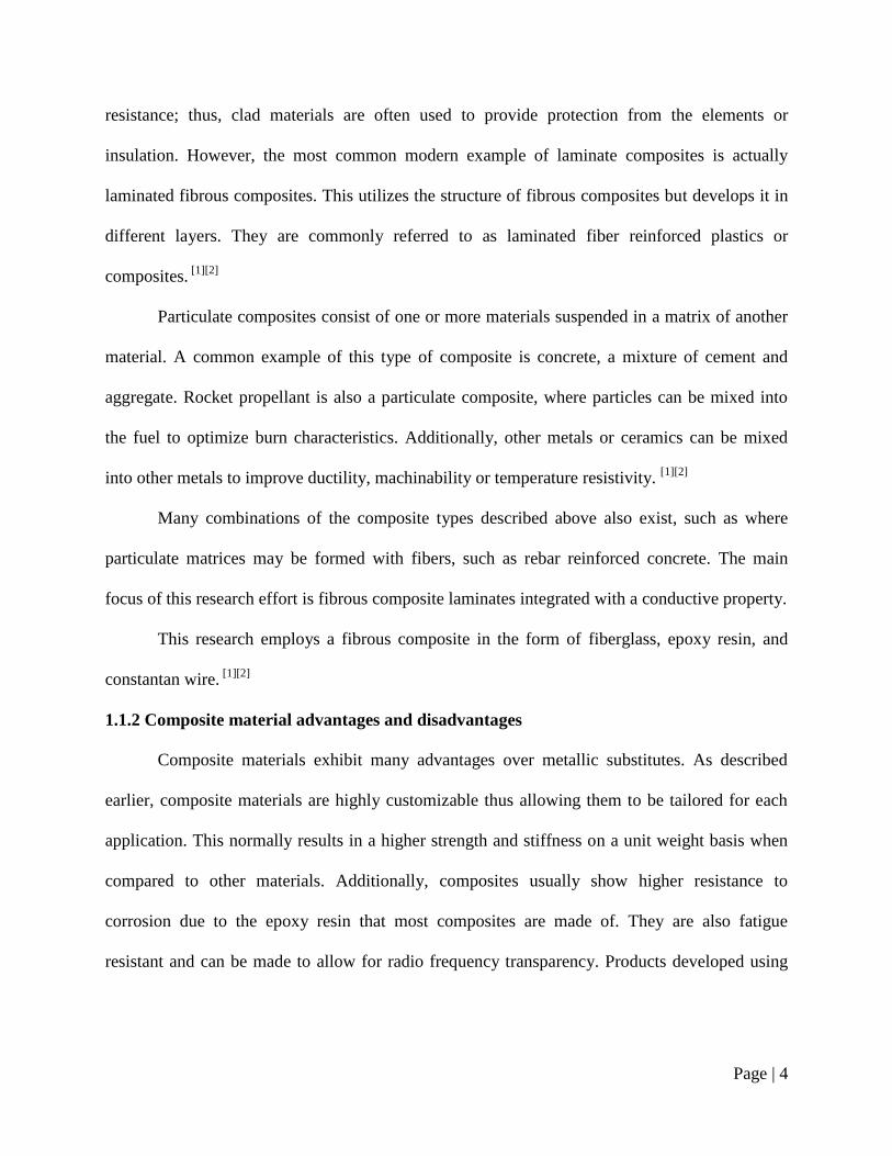
resistance; thus, clad materials are often used to provide protection from the elements or
insulation. However, the most common modern example of laminate composites is actually
laminated fibrous composites. This utilizes the structure of fibrous composites but develops it in
different layers. They are commonly referred to as laminated fiber reinforced plastics or
composites. [1][2]
Particulate composites consist of one or more materials suspended in a matrix of another
material. A common example of this type of composite is concrete, a mixture of cement and
aggregate. Rocket propellant is also a particulate composite, where particles can be mixed into
the fuel to optimize burn characteristics. Additionally, other metals or ceramics can be mixed
into other metals to improve ductility, machinability or temperature resistivity. [1][2]
Many combinations of the composite types described above also exist, such as where
particulate matrices may be formed with fibers, such as rebar reinforced concrete. The main
focus of this research effort is fibrous composite laminates integrated with a conductive property.
This research employs a fibrous composite in the form of fiberglass, epoxy resin, and
constantan wire. [1][2]
1.1.2 Composite material advantages and disadvantages
Composite materials exhibit many advantages over metallic substitutes. As described
earlier, composite materials are highly customizable thus allowing them to be tailored for each
application. This normally results in a higher strength and stiffness on a unit weight basis when
compared to other materials. Additionally, composites usually show higher resistance to
corrosion due to the epoxy resin that most composites are made of. They are also fatigue
resistant and can be made to allow for radio frequency transparency. Products developed using

Page | 5
composite layup techniques also have far fewer parts. There are no fasteners or labor associated
with joining parts. This can sometimes reduce cost depending on the application. [1][2]
However, composite material cost is normally more than aluminum or steel substitutes.
Additionally, the capital necessary to buy and make molds for composite layups can be more
expensive than machining metal parts. Thus, cost can be an advantage or disadvantage
depending on the application. Another significant disadvantage includes difficultly of repair.
Because fibrous composites lose strength if the fiber in the matrix is compromised, it is often
very difficult to repair and sometimes results in complete replacement of the part. Additionally,
damage is often non-visible and may occur within the layers of the laminates. Thus expensive
sonograph or x-ray tools are necessary to achieve any type of damage analysis. Lastly,
recyclability of composites is more complex than materials such as aluminum alloys which can
be melted and remade into new parts. Currently, there is still no effective and widely used way to
recycle modern composite parts.
With the evident difficultly of determining damage to composite structures, this research
effort attempts to simplify techniques by developing a nervous system for the structure during
the manufacturing process. Such a method can greatly improve the disadvantages of composite
materials associated with non-visible damage and structural health.
1.1.3 Fibrous Composite Weave Varieties
Weaving is a method of combining multiple fibers into a fabric or cloth by use of a loom.
This process dates back to ancient times using materials such as flax, wool or linen. Most
modern high tech woven fibers like carbon or glass are purchased in a plain or twill weave,
shown in Figure 3. The weaving pattern of a composite can play a very important role in the
strength and look of a structure. Additionally, the weave may serve as an essential method for

Page | 6
incorporating electrotextiles or sensors into a fabric for use of structural health monitoring.
Interweaving conductive elements as part of the fabric may serve as the sensory network of the
material. [3]
In this research constantan is used on a plain woven fiberglass; however, carbon is also
experimented with. Carbon is an already popular fiber due to strength but has significant
untapped conductive properties.
1.1.4 Manufacturing processes
Composite materials are fabricated in a variety of ways. One way to manufacture a
composite structure is by hand. The process, commonly known as hand lay-up, starts by creating
a mold to the like of the desired structure. A gel may be applied and rolled into the mold,
commonly made of tooling material like foam, to ensure good contact; the gel will provide a
good surface for the composite material to be applied to. Often times aluminum is used as a
mold. It provides excellent thermal transmission to assist in resin cure cycles. Additionally,
because the surface is already smooth after machining, a gel coat is usually not necessary but
normally a wave or release is applied. Hand lay-up materials require the use of dry fiber
materials, in the form of fiberglass, carbon fiber, or natural fiber. The resin is applied separately
by use of a roller or applicator similar to a spatula. The resins normally come in two parts and
Plain Twill Satin
Figure 3. Weave varieties

Page | 7
must be mixed in exact quantities to provide good curing. The dry fiber to resin content ratio is
also very important for developing a high strength and lightweight part. Parts made this way
normally require considerable consumable materials in the form of peel-plies, vacuum bags, and
breather cloths as well. A typical wet layup setup for vacuum bag pressure is shown in Figure 4.
[1][2]
Another technique of composite manufacturing is spray lay-up. A chopper head may be
used for quick fabrication. The chopper head sprays short fibers and resin simultaneously. This
results in a weaker product, but it is a much easier and faster fabrication process. Spray lay-up
requires the proper tools and the health hazards are even more evident due to the vaporous
component of the process.
Pultrusion is a process where the fiber reinforcements are drawn through a resin bath
where the material is coated and impregnated with resin. The reinforcements are then pulled
through a heated die to shape the fibers into the final shape of the part. This method is common
Figure 4. A typical wet layup setup

Page | 8
for creating composite rods or bars. A machine which accomplishes this is shown in Figure 5.
This process has a cost disadvantage, as the equipment used to manufacture by pultrusion is
normally relatively expensive. However, the process results in low cost for high quantity of parts
once the machine is purchased. [1][2]
Resin transfer molding or
RTM is a method where dry
fiber reinforcement is clamped
between two mold surfaces.
Resin is then injected under
pressure into the fiber
reinforcement. This method is
capable of using continuous,
chopped, or woven fibers. RTM
processing can quickly make parts, however, the molds require some investment. Thus high
production quantities are necessary to recover costs. Additionally, a mold may only make a
single part, so any alterations are extremely limited. [1][2]
There are numerous different techniques to developing composite structures; those
described above are just some common methods. This project utilized pre-preg fiberglass in a
heated press to create laminate plates and coupons. The pre-preg fabrication method utilizes
fibers already impregnated with the optimized amount of resin. Pre-preg sheets have a good ratio
of fibers to resin because they are created by reputable manufacturing companies that specialize
in optimizing the resin to fiber ratio. These types of sheets are often chilled in a refrigerator to
prevent the resin from curing at room temperatures.
Figure 5. Pultrusion composite part manufacturing
machine

Page | 9
Poor fabrication in either method may lead to voids. The voids will result in a weaker
structure. Some sources of voids are air bubbles, out-gassing and poor application of resin on
fibers. The operator should take extra time working out sources of voids to ensure a quality
product.
The structural health monitoring system in this research can be applied to nearly any
composite manufacturing process. Because it can be integrated, or woven directly into the
structural fiber weave it can be used either during a hand layup or prepreg applications. Curing
parts under severe temperature may result in melted or damaged sensors, depending on the
material.
1.2 STRUCTURAL HEALTH MONITORING SYSTEMS
The principal types of damage and failure that occur in composite structures are process
induced defects from porosity or delaminations. A second form is damage occurring during
assembly due to improper drilling of holes, forced fits and other inadequate processing. Thirdly,
damage can occur during the service of the structure. To reduce these types of risks, generally
parts go through extensive nondestructive testing methods prior to going in to service or repair.
However, these methods are often
time consuming and result in
downtime of composite vehicles.
Thus, a structural health
monitoring system is an ideal
method of addressing these issues.
Various traditional and popular
structural health monitoring
Figure 6. Fiber Bragg grating system

Page | 10
systems will be discussed.[4][5][6][7][8][9]
1.2.1 Fiber Bragg
Fiber Bragg grating (FBG) is a type of reflector used in waveguides such as optical
fibers. These types of reflectors are called Bragg reflectors. They utilize alternating materials
with a varying refractive index to induce partial reflection of an optical wave. Fiber Bragg
wavelengths are sensitive to strain and temperature, which makes them perfect for sensing
elements in optical fibers. As strain or temperature changes it causes a shift in Bragg wavelength,
allowing it to serve as a structural health monitoring device.[10][11][12][13][14][15]
Shown in Figure 6 is how a typical Fiber Bragg grating system would be used to measure
strain. As the fiber becomes strained the measured wavelength shifts due to changes in
reflections within the fiber; thus it is correlated with strain/stress.
1.2.2 Piezoelectric
Piezoelectricity is used in a variety of methods for structural health monitoring. It works
by analyzing the charge that is stored in certain materials. Piezoelectric sensors use the
piezoelectric effect, or the resulting charge or voltage from mechanical stress, in order to
measure pressure, strain, force or acceleration.
Piezoelectric sensors can be
coupled with lamb waves to measure
amplitude and phase changes in solids.
Lamb waves are popular in ultrasonic
testing to find flaws in objects. The
flaws are detected by reflections or
scattering that occurs from the
Figure 7. Piezoelectric patch transducers

Page | 11
imperfections, these scattered waves propagate back to the unit which measures the intensity.
Thus, a reading on the flaws can be determined.[16][17]
For example, vibrations in a piezoelectric transducer can be induced by a controller.
When connected to an array of other transducers, a signal pattern for damaged and undamaged
materials can be measured. A controller can then measure the system and collect information
regarding the condition of the material. Often times this type of system can be active, providing
electrical signals to dampen the vibrations.
1.2.3 Resistance & Strain Based
Many structural health monitoring methods involve the use of sensors. For example, strain
gauges use resistance measurements to correlate to strain. Similarly, embedded sensors can be
used to measure strain and temperature without applying a strain gauge. Additionally, if the
structure is not completely insulative, the entire part can be used to measure resistance. Of all the
structural health monitoring systems, resistance and strain based systems receive the least
attention. [18]
A goal of this research is to demonstrate the feasibility and usefulness of an interwoven
embedded system to provide structural health to a user at any given time, thus, further
developing the field of resistance based monitoring.
1.3 ELECTROTEXTILES
Embedded sensors are commonly made from metallic materials. However, there are also
many conductive textile products that could be used as sensors which may integrate better into a
fibrous composite than their metallic counterparts. Textile based composites have been heavily
used in recent years for their high strength, light weight, and electromagnetic properties.
Synthetic fibers like carbon fiber or fiberglass are commonly used, but there are many examples

Page | 12
of natural fiber composites as well. When additional electromagnetic protection or radio
frequency properties are desired an electrotexile may be used to alter the resistivity in the
composite. Commonly used naturally conductive materials are copper, aluminum, or ferrous
alloys; they are normally used as wires which is very similar to the size of a fiber tow. Carbon
fibers are also naturally conductive which presents the potential of using them as a conductive
element of the woven fabric. Even though
they are used for the excellent strength to
weight, they may also be used for electrical
properties; thus, allowing this research to be
applied to many already existing materials
and applications.
To develop a conductive fiber, a
nonconductive substance may be augmented
with small parts of conductive fiber as well.
This can be done during a spooling process
when the fiber is made, or the nonconductive
fiber can be dipped into a conductive coating.
For example, shown in Figure 9 is a
conductive yarn produced from 60%
polyester and 40% Inox steel fiber, a
conductive element.[19]
In this research, constantan is used as
an electrical element to simulate an
Figure 8. Spool of constantan wire, non-
insulated.
Figure 9. Electrotextile yarn made from
polyester and Inox steel fiber

Page | 13
electrotextile. Constantan is a copper nickel alloy consisting of 55% copper and 45% nickel. It
normally comes in a spool of wire, shown in Figure 8, very similar to how any fibrous textile tow
would be packaged. The similar shape allows the constantan wire to be easily incorporated into
the nonconductive structural elements of the composite. In this research, fiberglass serves as the
structural fiber element of the composite because of its insulating properties. However, utilizing
electrotextiles could be of great importance in future work. Thus, even though a more traditional
material was chosen for this study, the potential of other materials and their advantages should be
noted.
1.4 NONDESTRUCTIVE TEST METHODS
The only practical alternative to structural health monitoring is nondestructive testing
(NDT). This allows a user to investigate the structural integrity of a part without damaging it. If
the part is good it can return to service, otherwise it can be repaired or scrapped before any
catastrophic failures occur. Destructive testing is still one of the best ways to determine the
structural integrity of a part; however, when the testing is complete the part is destroyed so it is
not realistic to test parts this way. Nondestructive testing has both benefits and drawbacks when
compared to structural health monitoring. Normally the testing equipment is completely separate
from the part, so the part does not acquire any additional
weight or complexity during fabrication. However, it can
be extremely time consuming to investigate a large part
by a nondestructive testing method. Structural health
monitoring could provide a way to quickly test a large
part for structural integrity. Because nondestructive
testing and structural health monitoring are fairly closely
Figure 10. Cracks are revealed
by liquid penetration testing

Page | 14
related, an introduction to the many types of NDT is presented.[20][21][22]
1.4.1 Liquid Penetrant
Liquid penetrant is a very old technique normally used in aircraft maintenance. A
physical and chemical procedure is used to detect surface discontinuities in nonporous materials.
The process works by creating a contrast between a flaw and its background. Developer reveals
the evidence of cracks, porosity, or other discontinuities. It is fairly cheap, portable, and can be
automated. However, it only makes sense to test small parts and only works on the surface. Thus
interior delaminations would never be detected. An example of how liquid penetrant is used to
reveal a crack is shown in Figure 10.[20][21][22]
1.4.2 Magnetic Particle
Magnetic particle testing is another
method for detecting surface flaws and sub-
surface flaws in ferro-magnetic materials. The is
done by magnetizing the part, creating a
magnetic flux. Discontinuities result in a
distortion of magnetic flux which indicates a
flaw. Fluorescent or black oxide particles can
be used in conjunction with magnets to
uncover flaws. The method works well for
metals that can be magnetized. It is also simple
and can be applied to shafts, engines or hard to
reach areas. However, in a composite
application it does not work well because
Figure 11. Magnetic flux is distorted by
flaws
Figure 12. Flaws reflect ultrasonic waves
during Ultrasound NDT

Page | 15
composites are not ferro-materials.[20][21][22]
1.4.3 Ultrasonic
Sound above the limit of audibility is referred to as ultrasound, in the frequency range of
0.2 MHz to 800 MHz. Ultrasonic inspection provides a sensitive method of nondestructive
testing in nearly any material. It is capable of estimating the location and size of the defect via
only one accessible surface. The method operates on the principle of transmitted and reflected
sound waves. Sound has a constant velocity in a given substance, thus changes in the acoustic
impedance of the material results in a velocity change in the sound wave. The distance of the
flaw can be determined by the time taken for the sound wave to return. There are a variety of
different kinds of ultrasonic inspection such as pulse echo and transmission techniques.
Ultrasonic is a dependable method for obtaining accurate results of flaws. However, it requires
calibration standards and trained operators. A typical ultrasonic NDT test setup is shown in
Figure 12. [14][15][20][21][22]
1.4.4 Radiography
A radiograph is a photographic record produced by the passage of electromagnetic
radiation such as x-rays or gamma rays through an object onto a film, the same way x-rays are
taken in the medical field. These methods require equipment to produce x-rays or gamma rays. X
-rays require a source of electrons and means of propelling them at high speeds through the
object. Gamma rays on the other hand are generated by the disintegration of radioactive
substances such as Iridium-192 or Cobalt-60. Gamma ray equipment is normally simpler than x-
ray equipment. Radiography provides good penetration on a large variety of material types.
However, it also requires trained personnel. Additionally, radiation is a hazard and personnel
should not be in the area when it is being used.[20][21][22]

Page | 16
1.4.5 Thermography
Thermography is based on the principle
that heat flow in a material is altered by the
presence of anomalies. The changes in heat flow
cause localized temperature changes. Imaging the
thermal patterns reveals flaws in the material.
This is normally done with infrared waves. The
frequency and wavelength of the radiation can be correlated closely with the heat of a radiator.
This process requires significant equipment, a thermal imager, detector scanning system, and
more. It can be used to detect many different types of voids and is flexible enough to be used on
fluids as well. However it also requires trained personnel and significant capital for
equipment.[20][21][22]
1.4.6 Nondestructive Test Methods Summary
There are many more methods that have not been presented. However, it is evident that
some NDT methods work better for fiber reinforced composite materials than others. Defects in
fiber materials are often difficult to detect and may arise from the raw product, during the
fabrication process or while in service. A table from Nanyang Technological University in
Singapore has been recreated in Table 1 and summarizes the capabilities of each of the major
NDT techniques.[21]
Figure 13. Thermographic image of
delaminations in a fiber reinforced
composite

Page | 17
Table 1. Composite defects which can be detected by various NDT techniques
Defect Type Ultrasonics Radiography
Eddy
Current
Acoustic
Emission Thermography
Optical
Holography
Mechanical
Impedance
Voids, porosity Yes Yes
Some Some Some
Debonds Yes Some
Some Yes Yes Yes
Delaminations Yes Some
Some Yes Yes Yes
Impact damage Yes Yes Yes
Some Some Some
Resin
variations Yes Some
Broken fibers Yes Some Yes Yes
Fiber
misalignment Yes Yes Yes
Resin cracks Yes Some
Yes Yes Yes
Cure variations Yes
Inclusions Yes Yes
Moisture Yes
1.5 LITERATURE REVIEW
A variety of structural health monitoring studies were reviewed. The most popular and
available studies utilized Fiber Bragg grating, piezoelectric and Lamb waves. Very few were
resistance or strain based. However, a few relevant studies were completed and are described in
this section.
Structural Health Monitoring by Electrical Resistance Measurement by D.D.L Chung of
State University of New York in Buffalo[23]
, was one of the few studies available specifically
studying resistance based SHM. The author utilizes a theory of volume electrical resistivity to
detect structural changes in bulk materials. Resistance can be measured across the entire
component as long as the material is not completely insulative. This can be done real-time with
no sensors. In a graphite/epoxy laminate the fibers are conductive. Within a single lamina there
is a finite number of adjacent fiber contacts, this creates a specific path of resistance. Between
lamina within the laminate there are also a finite number of contacts in the through-thickness
direction. The summation of the resistance these contacts develop is the volume resistance. The

Page | 18
author uses the four-lead Kelvin resistance measurement technique to measure resistance
changes between fiber contacts within a lamina and between lamina within a laminate under
different types of mechanical degradation. Chung showed the effectiveness of using graphite
fibers as a conductive sensor element within a laminate. This is very similar to the goals of this
study; however, the author used a different approach.
Strain-based Structural Health Monitoring of Complex Composite Structures by Ajay
Kessavan, Sabu John, and Isreal Herszberg of RMIT University in Melbourne, Australia[18]
was
another paper that was reviewed. The authors developed a system in order to address the evident
composite material disadvantages of matrix cracking and delamination. Using traditional strain
sensors, they developed a neural network within a fiberglass T-joint structure. The sensors were
adhered over the component, not embedded. The system is based on the principle of load paths.
Change in load paths occur during delaminations or fractures, which results in a change of strain
measurements. The software the authors developed measures degraded strain values and
compares them to a healthy reading. With a significant number of sensors the system is capable
of predicting the sizes and locations of delaminations within the T-joint part. The authors showed
that using a large number of sensors, a neural network can be developed to determine size and
location of damages. This is a future goal of this study, albeit a different mode of sensing.
Structural Integrity of Composite Laminates with Embedded Micro-sensors authored by Yi
Huang and Sia Nemat-Nasser from UC San Diego[24]
, was also reviewed. The authors researched
the mechanical consequences of embedding micro-sensors within a composite structure. They
developed a finite element model to analyze a case of an embedded sensor. For sensors of
significant thickness, 1/7 scale of the length, load is distributed around the sensor. Their model
predicted premature failure due to stress concentrations created by the corners of a rectangular

Page | 19
sensor. However, they concluded that sensors that do not alter the through-thickness significantly
have neglible effects on the material integrity. The authors showed that embedding large micro-
sensors may compromise structural integrity. However, in this study, A Resistance Based
Structural Health Monitoring System for Composite Structure Applications, the through-
thickness is not affected and the sensors are round. Thus it can be concluded they do not have an
effect on the structural properties of the test specimens developed in this study.
1.6 SCOPE OF WORK
This research encompasses the use of a conductive fiber element integrated into a
nonconductive fiberglass composite structure for use in structural health monitoring. The main
objective of this study is to develop a simple method for measuring deviations from baseline
health and identifying potential catastrophic events of a composite laminate by utilizing an
integrated resistance based measuring system.
Chapter 1 provides background information and introduction to composites, structural
health monitoring and this research effort.
Chapter 2 describes the theory of the structural health monitoring system. It presents the
idea and design process that led to the development of the strain based structural health
monitoring system. Additionally, it describes the test equipment and software used to obtain data
for health monitoring.
Chapter 3 describes the manufacturing processes for the test specimens used in this
research. This research is to test the theory of utilizing an integrated conductive fiber element in
the form of a constantan wire into a composite laminate for structural health monitoring. The
integration of the sensor element involved specific manufacturing and process; thus, methods to

Page | 20
best integrate the sensor are developed. In addition, the length and orientation of constantan wire
was varied to determine a relationship to the sensitivity of the measurements.
Chapter 4 describes the results for each test case. Plots present the correlation between
strain and resistance. Discussion of the results is also provided.
Chapter 5 presents correlation with an analytical approach using equations and theory
from Chapter 2. These solutions are compared to experimental results presented in Chapter 4.
Chapter 6 provides a conclusion, importance of work, and suggestions for further
improvement of the system.

Page | 21
CHAPTER 2. THEORY OF SYSTEM
The structural health monitoring system developed in this research is presented in this
chapter. The methodology of the system is discussed from elementary strain gauge theory and
extended to the composite manufacturing process. The issues and processes for developing such
a system are also presented.
2.1 SYSTEM ARCHITECTURE
The structural health monitoring method described in this study utilizes a conductive
fiber interwoven with a nonconductive fiber and embedded in a matrix to develop a composite
laminate. The conductive fiber, a single continuous constantan wire, serves as a sensor in the
structure by measuring resistance changes in the wire under various loading cases. The
nonconductive fiber serves as a structural fiber element. This approach can be accomplished by
using other conductive fiber elements, such as carbon or copper; however, most of these
materials exhibit variations in temperature and resistance. Thus, to develop a straightforward
and viable study, the fiberglass was used in conjunction with the constantan wire. This idea can
be expanded to use solely carbon fiber as the conductive and nonconductive element in the
future.
To simplify the objective of testing this method as a viable option for structural health
monitoring, the constantan wire was embedded within the fiberglass plies rather than interwoven
with them. Weaving them into the fabric would require starting from a tow and utilizing a loom
to combine both elements. Currently, no weaves are readily available that consist of conductive
and nonconductive fibers interwoven.
A variety of manufacturing processes were developed. Each resulted in advantages and
disadvantages for using the strain sensor. Three main processes were used, full length wires

Page | 22
protruding from each end, a parabolic shaped sensor with leads protruding from one end, and a
threaded through specimen which resulted in leads out the side. Each of these is discussed in
more detail in Chapter 3. The lead wires are connected to an Agilent micro-ohm-meter and data
acquisition measurement device that measures the resistance values of the constantan wire. The
change in resistance values is small due to the length and cross sectional area of the wire. Thus a
measurement device with sufficient accuracy is required. The resistance values can be
transformed into strain and stress values by use of strain gauge theory explained in the following
section.
2.2 STRAIN GAUGE THEORY
The structural health monitoring method described in this study borrows many ideas from
the strain gauge, a widely used measurement device. Normal strain is defined as the amount of
deformation per unit length when a load is applied to an object. Thus, normal strain is calculated
by dividing the total deformation by the original length as shown in Equation 1.
Strain ≡ ε = ∆LL
Equation 1: Strain
Strain is normally very small and expressed in micro-strain. It is also unit-less, but is
often expressed as inch/inch. The strain may be negative or positive which denotes a
compressive or tensile load, as shown in Figure 14. Strain gauges work by converting
mechanical motion into electrical signals. When a wire in a strain gauge is under tension the wire
slightly lengthens and the diameter cross section is reduced. Shown in Equation 2 is the
commonly used equation for resistivity of uniform cross section materials, such as wires.
R = ρl
A
Equation 2: Resistance
Page | 23
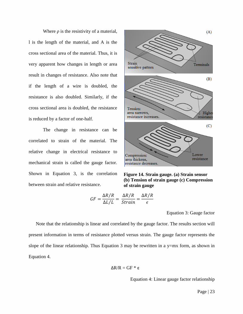
Where ρ is the resistivity of a material,
l is the length of the material, and A is the
cross sectional area of the material. Thus, it is
very apparent how changes in length or area
result in changes of resistance. Also note that
if the length of a wire is doubled, the
resistance is also doubled. Similarly, if the
cross sectional area is doubled, the resistance
is reduced by a factor of one-half.
The change in resistance can be
correlated to strain of the material. The
relative change in electrical resistance to
mechanical strain is called the gauge factor.
Shown in Equation 3, is the correlation
between strain and relative resistance.
𝐺𝐹 =∆𝑅 𝑅
∆𝐿 𝐿 =
∆𝑅 𝑅
𝑆𝑡𝑟𝑎𝑖𝑛=∆𝑅 𝑅
𝜖
Equation 3: Gauge factor
Note that the relationship is linear and correlated by the gauge factor. The results section will
present information in terms of resistance plotted versus strain. The gauge factor represents the
slope of the linear relationship. Thus Equation 3 may be rewritten in a y=mx form, as shown in
Equation 4.
ΔR/R = GF * ε
Equation 4: Linear gauge factor relationship
Figure 14. Strain gauge. (a) Strain sensor
(b) Tension of strain gauge (c) Compression
of strain gauge

Page | 24
The gauge factor can also be calculated from resistivity and Poisson’s ratio,𝜐, given in
Equation 6.
𝐺𝐹 =∆𝜌 𝜌
𝜖+ 1 + 2𝜐
Equation 5: Gauge factor from resistivity
Normally for most applications the resistivity can be assumed to be constant. In the case of
piezoresistive materials, the resistivity, ρ, of the material is not constant. Thus, Δρ/ρ represents
the piezoresistive term. However, a more exact solution for the gauge factor takes into account
temperature, such as presented in Equation 6.
𝐺𝐹 = (∆𝑅
𝑅− 𝛼𝜃)
1
𝜀
Equation 6: Gauge factor variation due to temperature
Where R is resistance, α is the temperature coefficient, ε is strain, and θ is temperature
change. Expanding or contracting of the material can lead to changes in resistance, which can be
the result of temperature change. However, that is not the only result of temperature change.
Activity of atoms within the material changes; thus, the material property of resistivity may also
change. In general, conductors tend to increase resistivity due to an increase in temperature.
These changes can result in inaccuracies of measurements for resistance, and consequently,
strain. By using constantan as the conductive fiber element to act as a strain sensor the
temperature issue is addressed. Constantan gets its name from maintaining a constant resistance
with varied temperatures. It is a material already commonly used in most strain gauges.[25]
Often strain sensors are attached directly to the surface of a structure using an adhesive,
which may be done poorly and result in inadequate readings. By embedding the strain sensor
within the composite laminate during manufacturing, the issue of bonding is easily addressed.

Page | 25
This process results in improved bonding over the alternative of adhesion over a surface affixed
strain device.
Commonly used strain gauges are made of metallic foils that are extremely small and
measure strain over a very small area. This is ideal for measuring strain accurately and precisely
at desired locations. However, for measuring average strain of a part over larger areas it is less
effective. An additional benefit of using a sensor that is interwoven with the composite laminate
is that it covers more area. Thus, even though it is not necessarily more accurate it can generalize
strain over a larger area.
2.3 EXPERIMENTAL TESTING METHODS
Testing standards are developed for international coherence and consensus of technical
information. The standards develop a medium which allows work to be compared with
significance. In the field of composites many standards are used. Many are developed by
companies such as Boeing or NASA. However, one of the most widely used is a public testing
standard, ASTM International
The American Society for Testing and Materials (ASTM) is a global leader in the
development of testing standards. The compilation of ASTM standards includes testing methods
for a wide variety of subjects, from chemistry related projects to imaging, construction or water
testing. Their database includes over 100 areas of interest and 12,000+ standards covering
metals, petroleum, construction and more. Under lamina and laminate test methods, ASTM
provides twenty relevant testing methods for tension, compression or flexural strength of a
sample.
For this experiment, D3039 Standard Test Method for Tensile Properties of Polymer Matrix
Composite Materials will be used[26]
. Any testing method could be used to test the effectiveness
Page | 26
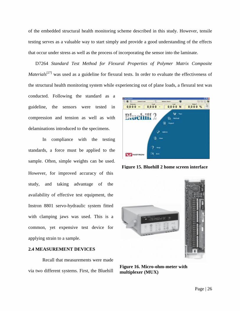
Figure 15. Bluehill 2 home screen interface
of the embedded structural health monitoring scheme described in this study. However, tensile
testing serves as a valuable way to start simply and provide a good understanding of the effects
that occur under stress as well as the process of incorporating the sensor into the laminate.
D7264 Standard Test Method for Flexural Properties of Polymer Matrix Composite
Materials[27]
was used as a guideline for flexural tests. In order to evaluate the effectiveness of
the structural health monitoring system while experiencing out of plane loads, a flexural test was
conducted. Following the standard as a
guideline, the sensors were tested in
compression and tension as well as with
delaminations introduced to the specimens.
In compliance with the testing
standards, a force must be applied to the
sample. Often, simple weights can be used.
However, for improved accuracy of this
study, and taking advantage of the
availability of effective test equipment, the
Instron 8801 servo-hydraulic system fitted
with clamping jaws was used. This is a
common, yet expensive test device for
applying strain to a sample.
2.4 MEASUREMENT DEVICES
Recall that measurements were made
via two different systems. First, the Bluehill
Figure 16. Micro-ohm-meter with
multiplexer (MUX)

Page | 27
2 software made by Instron for material testing applications was used to measure strain. This
study investigated the tensile and flexural effects on an embedded structural health monitoring
device utilizing a constantan wire element. The software provides an easy to use interface and
presents test data clearly. Secondly, An Agilent 34420a micro-ohm-meter was used to measure
resistance values and correlate them with strain. Thus, two independent systems were used. In
the field, measurements would be made via the ohm-meter only. The Agilent meter uses a four
wire Kelvin resistance measurement by use of four banana-alligator connectors. The alligator
connectors attach directly to the leads of the embedded wire. Software for the ohm meter was
written in Visual Basic through Excel.[28]
Other devices and software can be used for this experiment such as LabView or C. In a
real application, a multiplexer, a device that selects one of several available input signals, would
likely be wired directly to multiple leads in the structure to transmit a multitude of signals to the
monitor. This method would provide data over a greater area and for the overall structure; thus,
providing continuous data to a monitor where a user
can review structural health.
Details of the measurement devices and test
setup for experiments are discussed further in
Section 4.2.
2.5 SYSTEM DESIGN
The structural health monitoring system
discussed in this research provides the foundation
for future work. Because this study was analyzing
the fundamental aspects of the sensor and not the
Figure 17. Woven fabric showing
warp and weft fibers

Page | 28
entire system, there are many applications to investigate. Additionally there are numerous
different ways to employ the system developed during this research study. Some of these
different ways are discussed.
During this study, the sensor was embedded between two nonconductive woven layers.
However, in a truly interwoven specimen the conductive fibers will exist in the same layer. This
can easily be done on most looms which are already in widespread use to develop the weave
patterns purchased by manufacturers. By weaving plain fibers with a warp and main weft with
use of a loom and inserting the wire as a supplementary weft or warp at regular intervals a
completely interwoven layer can be developed. Thus, when developing a composite laminate, the
interwoven sensory layer can be used and separated by an insulation layer from other conductive
layers or elements. On the other side of an insulation layer a similar SHM layer can be placed at
a ninety degree orientation. This develops a grid that can measure resistance values in a 2-D
plane. The grid points would be spaced by as many leads as necessary for accuracy in the
structure. The leads can then be connected to a multiplexor. By using a DAQ measurement
device, strain can be continuously measured along the x-axis and y-axis simultaneously from
each lead. The leads that exhibit the highest strain on the x-axis can be associated with the
highest strain on the y-axis. This allows a user to develop a plane to pinpoint where stress is
occurring on the structure. Having a system that can approximate the location where damage is
on a structure can be extremely helpful, especially if the structure is very large.
Additionally, the system is capable of determining the type of stress. A negative value
may denote compression, whereas, high positive values could denote pressure forces from the
opposing side. Additionally, if the system is continually monitored, it can determine events such
as an impact or collision. If an open circuit is detected it may indicate a puncture in the structure

Page | 29
which has destroyed the continuity of the conductive elements. Thus, users can have real-time
structural health measurements that allow them to infer what issues may be occurring.
The system can also be used to measure deviations from baseline structural health values.
By measuring values using the integrated system prior to use, a user can determine if any
deviation of structural health occurs in the structure throughout its lifetime. When resistance or
strain values approach a limit that may indicate fracture, maintenance can replace the part before
any catastrophic damage occurs. This is very important for composite parts which are difficult to
analyze while in use. Many times perfectly good parts are removed prior to their end of life and
replaced, however, a system that can provide continuous health monitoring is capable of
determining when exactly the components should be replaced; thus, saving time and costs
associated with maintenance in many applications.
These ideas present some of the ways this research can be utilized to provide a better
understanding of composite materials while in the field. It serves as a way to maintain safety and
improve quality of composite parts while also reducing costs associated with maintenance. Many
other applications are likely to exist which can be based upon this type of embedded sensor.

Page | 30
CHAPTER 3. MANUFACTURING PROCESS
The specimen manufacturing process will be discussed in this chapter. A detailed step by
step on the fiber preparation, curing cycle, and test preparation is presented. The conductive fiber
sensor and embedding process is also presented.
3.1 COMPOSITE LAMINATE PLATE PREPARATIONS
To simulate a composite structure, laminates are prepared. Fiberglass/epoxy prepreg is used
as the main structural element of the composite laminate. Sensors are then embedded within the
laminates for structural health monitoring.
3.1.1 Material Characteristics
The material used for the structural component of the composite laminate should be
simple, easy to manufacturer and be insulating as not to interfere with the conductive properties
of the strain sensor. For this application, a pre-preg fiberglass was the ideal choice for the
structural component of the specimen. Thus, the BT250E-1 Resin System in conjunction with
7781 "E" Fiberglass Reinforcement by TenCate was used for this purpose.
The BT250E-1 resin system displays good toughness and strength in a standard epoxy
matrix. It resulted in a shiny surface finish with a heated press cure and is a good choice for
applications in a low to medium service temperature. It has a shelf life of 30 days at 25°C and 12
months at 0°C. This product is normally used in secondary aircraft structures, racing vehicles,
radomes, reflectors, sporting goods, medical items, and general purpose composites. The
BT250E-1 Cirrus Optimized Epoxy that was donated by TenCate is actually the same material
used for Cirrus aircraft construction. It is a unique type of the 7781 "E" fiberglass because the
woven fabric is impregnated with resin on only one side. Thus, one side of the pre-preg remains
dry until the cure cycle begins. This helps during the layup process because the layers are easy to

Page | 31
position when dry. It also helps orient the fibers during the embedding process, otherwise they
would continually stick to the prepreg sheets as they were integrated. The resin and mechanical
properties of the fiberglass were supplied by TenCate as part of a technical data sheet and are
presented in Table 2.[29]
Table 2. Resin and Mechanical Fiber Properties
Resin Properties 7781 "E" Fiberglass Reinforcement
Density........................... 1.17 gm/cc Tensile Strength.................... 63.0 ksi
Tg................................... 125°C Modulus................................ 3.8 Msi
Dielectric Constant........ 3.0 @10Ghz Compressive Strength........... 70.6 ksi
Loss Tangent................. 0.019 @10Ghz Modulus................................ 3.2 Msi
Moisture Absorption...... 2.0% after 24hr boil Flexural Strength.................. 84.8 ksi
Tensile Strength............. 10.9 ksi Modulus................................ 3.2 Msi
Tensile Modulus............ 0.44 Msi Short Beam Shear Strength... 7.9 ksi
Tensile Strain................. 2.5%
Compression Strength... 16.7 ksi
Compression Modulus... 0.40 Msi
Flexural Strength........... 22.6 ksi
Flexural Modulus.......... 0.50 Msi
Flexural Strain............... 5.5%
The Tetrahedron heat press, shown in
Figure 18 was used for manufacturing of the
laminates. The resin used on the selected
material utilized a Tencate specified Cirrus
Optimized Epoxy 90600 Rev C cure cycle
provided by the manufacturers, shown in
Figure 19. The press was set to a heat-up rate
of 4°F/min, 180°F soak for 45 minutes, 260°F
dwell for 100 minutes and naturally cooled at
ambient temperature. A pressure of 1000
Figure 18. Tetrahedron Press

Page | 32
pounds across the 12”x12” plate was applied during the cure cycle, resulting in approximately 7
psi. The Tetrahedron heat press is a pneumatic press engineered for precision lab research and
prototype testing. It is capable of pressuring up to 1000 lbf with an accuracy of ± 1%, and
applying temperatures of up to 850°F with a temperature uniformity of ± 4°F.
Figure 19. BT250E-1 Cirrus Optimized Epoxy cure cycle

Page | 33
3.1.2 Laminate Preparation Process
The pre-preg fiberglass was purchased as a 56" wide roll. Shown in Figure 21, is the roll
being prepared to be cut into lamina, or individual sheets. The Tetrahedron press only has space
for a maximum size of 12"x12" area layups. Thus, the lamina was cut into 12.5"x12.5" sheets.
This was slightly larger than the area of the press, however, the 0.5" extra length allows for some
tolerance during the fabrication process.
Even so, not even the full 12"x12"
press area produces parts of
useable quality. Thus, this method
allows for, at best, ten 1" wide test
specimens after all preparations
are completed.
Layers are cut using a
handheld roller cutter along a
straight edge. Working from the
roll shown in Figure 21, a
horizontal 12.5" cut was made,
Figure 21. BT250E-1 Resin with 7781 "E" Fiberglass Reinforcement pre-preg
Figure 20. Prepared fiberglass lamina

Page | 34
developing a 12.5"x56" long strip. The 56" allows sufficient material to cut four layers. Thus,
also using a straight edge and cutter, four 12.5"x12.5" layers are fabricated, shown in Figure 20.
In addition, non-stick Teflon sheets are used between the fiberglass sheets and mold
surface of the press. This prevents the sheets from sticking to the mold and allows them to be
removed after the cure process. The Teflon sheets must be cut slightly larger than the lamina
sheets to prevent the excess resin from dripping onto the machine. In some cases these sheets
were actually very useful during the manufacturing process, described further in Section 3.2.
Next, the fiberglass laminates are paired up and
combined. Utmost care must be made to align the fibers
and even though the intention was to have a completely
symmetric, 0° by 90° layup, in reality it is impossible.
The two pairs will consist of the top and bottom of the
laminate, where the structural health monitoring device
will be inserted into the middle surface. Placing it here
will result in a more symmetric layup. Additionally, it
will see the least amount of out of plane stresses if they
somehow occur.
3.1.3 Delaminated Specimen Preparation Process
One objective of this study was to determine the
sensor effectiveness of detecting delaminations. Thus a
delamination was introduced to the composite laminate
during the layup process. This was in the form of a 1”
wide strip created by inserting a non-stick, non-porous
Figure 22. (left) Threaded
Through Linear Sensor (right)
With Delamination

Page | 35
Teflon sheet into the middle surface. The sensor was laid up directly on top, also in the middle
surface. This prevents bonding between the lamina in this area and results in a delamination.
Delamination samples were made for two cases: the threaded through linear tensile and
flexural cases.
3.2 CONDUCTIVE SENSOR PREPARATION
Following preparation of the structural lamina elements, the conductive sensor can be
integrated in the laminate. A variety of different methods can be used to integrate the sensor into
the specimens and test them. Collectively, ten different cases were analyzed. Some embedding
methods were found to be more effective than others and are described in detail. Additionally,
predictions of test results are made for some cases.
3.2.1 Material Characteristics
As mentioned, the sensor in this study was made of constantan wire. Constantan is a
copper-nickel alloy which normally consists of 55% copper and 45% nickel. It is commonly used
because of its unique resistivity characteristics. Constantan gets its name because its resistivity
remains constant over a wide range of temperature. The resistivity for constantan is relatively
high when compared to other metals. Thus, this metal is ideal for measuring changes in
resistance due to strain rather
than temperature; making it a
great choice for studying
stress-strain effects on a
composite laminate.[30]
Constantan is the
most widely used material for
Table 3. Constantan material properties
Material Property
Resistivity (70°C) 0.0000489 ohm-cm
Temperature coefficient (20°C) 8 parts-per-million Kelvin
Density 8900 kg/m3
Melting point 1221 to 1300 °C
Specific heat capacity 19.5 W/(mK)
Thermal conductivity 14.9 x 10⁻⁶
per Kelvin
Tensile strength 455 to 860 MPa
Elongation at fracture <45%
Elastic modulus 162 GPa

Page | 36
strain gauges and thermocouples. In addition to having very high insensitivity to temperature, it
has a fairly high strain sensitivity or gauge factor. This allows for more accurate readings during
strain measurements. It also has very good elongation characteristics which will allow it to
deflect significantly within the composite without fracturing. The physical properties for
constantan are presented in Table 3.
The diameter of the sensors was 0.010”. During integration of the constantan wire sensor
in the composite laminates a length of 18 inches was used for all linear sensors and 36 inches for
all parabolic sensors. This was to investigate the sensitivity and effectiveness of the sensor as it
related to length of the wire.
3.2.2 Full Length Linear Sensor
The first and most forward approach to integrating the sensor into the laminate was to
create a straight length of wire and protrude it from each side. These are placed in the center of
1” wide sections measured on the laminate plates, leaving space for about 9 or 10 sensor
samples. Some space was left between each 1” section to allow space during the machining
process and for the kerf of the blade, or the width of material removed during cutting.
During pilot studies of this method it was noted that the wires would become curved
when in the heated press. This was a result of significant pressure and the flow of resins out to
the side of the plate. This flow would cause the wires to bend outwards and result in specimens
with non-aligned sensors. This approach was resolved by putting tension on the wires while it
was curing. This was done by taping the sensors to the Teflon sheets at distances that were
slightly shorter than the actual wire, causing the Teflon sheets to bow. However, when the Teflon
sheets were flattened, it would put pressure on the wire sensors. Thus, once the plate was
inserted into the heated press, methods were employed to flatten the Teflon sheet to apply a

Page | 37
tensile force. This was done by using a water bottle as weight on the Teflon sheet. The weight
could be varied by how much water was inside the bottle, but a completely full 16oz bottle
worked effectively.
Once the samples were
completely cured, they were machined
into 12” by 1” samples. The entire plate
before the machining process was shown
in Figure 23. However, one end of the
plate could not be machined because the
leads protruded out the end. Thus this end
was left un-refined. It must be noted that
during the cure process the resin was squeezed out of the prepreg laminate. This resin would
have a tendency to build up around the wire protrusions developing an area of significant resin.
Because this normally occurred at the edge of the heat press, the samples were not always flat,
but slightly curved around the mold. Additionally, this area was nearly impossible to clean up
because of the possibility of damaging the sensitive wire.
During testing of these samples the pneumatic clamping jaws of the Instron would crush
this area with significant force. Normally this would cause a portion of the wire to shear off from
the rest of the wire still embedded within the laminate. Therefore, it became a useless test
specimen. As a result, it is not recommended to recreate this experiment with this fabrication
process unless these issues can be addressed. Moreover, a parabolic sample that had wire leads
protruding from the end was not created. It would likely result in the same difficulties as the
linear sensor.
Figure 23. Full length linear sensor

Page | 38
3.2.3 Threaded Through Linear Sensor
Another approach was taken to integrate the sensor into the laminate. This approach was
driven by three main purposes: first, to determine if the clamping jaws of the Instron had any
effect on the resistance measurements of samples; second, to improve machinability and develop
clean cut edges on the samples; third, to be more representative of an application.
These samples were developed by using a needle. Similarly to all the other specimens
they were laid up in the middle surface of the laminate. However, constantan was threaded
through the eye of the needle, then through
a marked surface on the lamina sheet,
shown in Figure 24. This marked surface
indicates the center of the 1” wide strip.
The wire was also threaded through a
porous non-stick sheet and a non-porous
Teflon sheet. These sheets ensure the wire
will not become infused with the outer
surface of the laminate during the cure
processes. Thus, a linear length of wire was created on one side of the laminate and the wires
protrude from the other side. The side with the linear length was placed against the other half of
the laminate into the middle surface. The lead side was laid flat against the non-stick sheet
surface. On top of this, a sheet of thick cotton was added to allow the wires to be absorbed into
the cotton and prevent the wires from creating crevices in the samples. During the cure process,
tension can be applied much the same way as previously. Using a weight, tension was applied
during the cure cycle to ensure that the wires are straight.
Figure 24. Preparation of the threaded linear
sensor
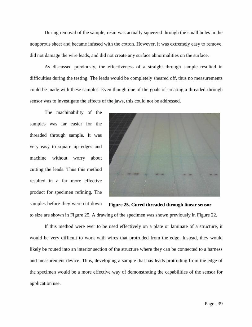
Page | 39
During removal of the sample, resin was actually squeezed through the small holes in the
nonporous sheet and became infused with the cotton. However, it was extremely easy to remove,
did not damage the wire leads, and did not create any surface abnormalities on the surface.
As discussed previously, the effectiveness of a straight through sample resulted in
difficulties during the testing. The leads would be completely sheared off, thus no measurements
could be made with these samples. Even though one of the goals of creating a threaded-through
sensor was to investigate the effects of the jaws, this could not be addressed.
The machinability of the
samples was far easier for the
threaded through sample. It was
very easy to square up edges and
machine without worry about
cutting the leads. Thus this method
resulted in a far more effective
product for specimen refining. The
samples before they were cut down
to size are shown in Figure 25. A drawing of the specimen was shown previously in Figure 22.
If this method were ever to be used effectively on a plate or laminate of a structure, it
would be very difficult to work with wires that protruded from the edge. Instead, they would
likely be routed into an interior section of the structure where they can be connected to a harness
and measurement device. Thus, developing a sample that has leads protruding from the edge of
the specimen would be a more effective way of demonstrating the capabilities of the sensor for
application use.
Figure 25. Cured threaded through linear sensor
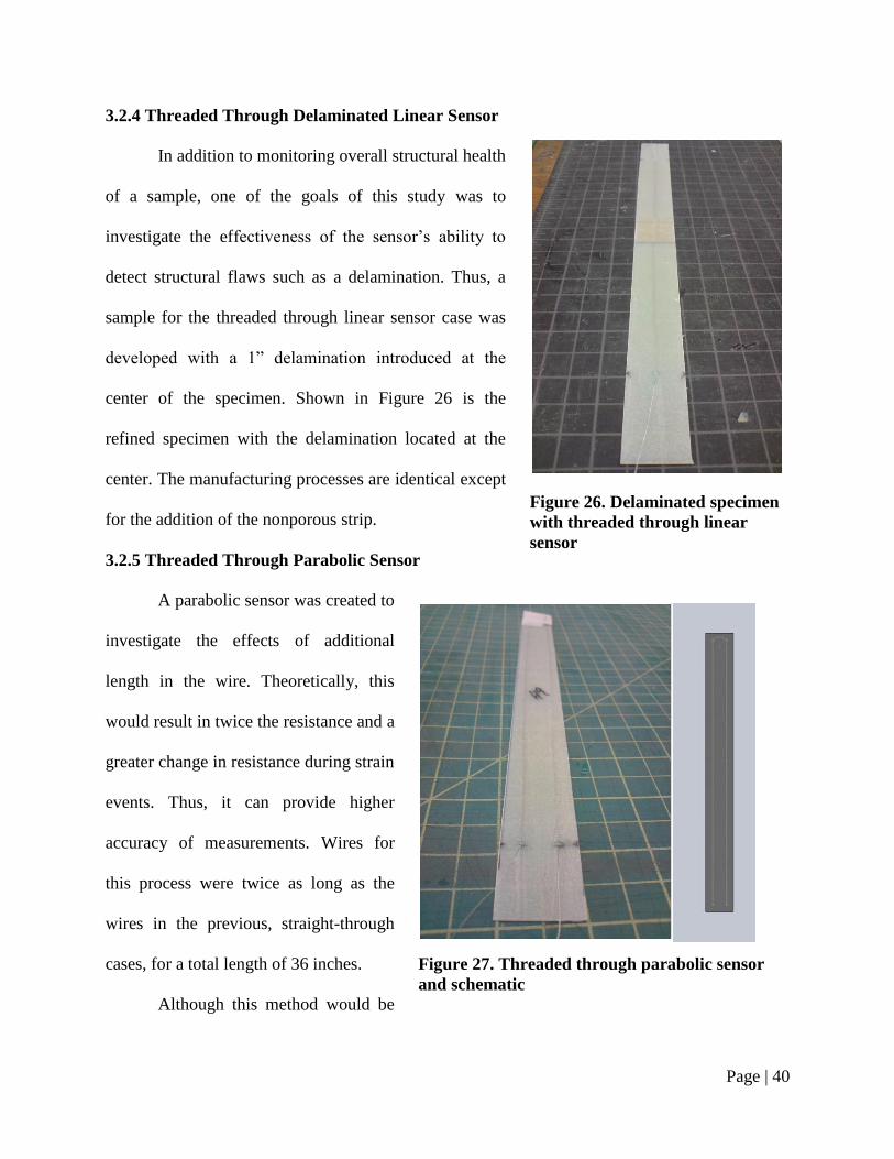
Page | 40
3.2.4 Threaded Through Delaminated Linear Sensor
In addition to monitoring overall structural health
of a sample, one of the goals of this study was to
investigate the effectiveness of the sensor’s ability to
detect structural flaws such as a delamination. Thus, a
sample for the threaded through linear sensor case was
developed with a 1” delamination introduced at the
center of the specimen. Shown in Figure 26 is the
refined specimen with the delamination located at the
center. The manufacturing processes are identical except
for the addition of the nonporous strip.
3.2.5 Threaded Through Parabolic Sensor
A parabolic sensor was created to
investigate the effects of additional
length in the wire. Theoretically, this
would result in twice the resistance and a
greater change in resistance during strain
events. Thus, it can provide higher
accuracy of measurements. Wires for
this process were twice as long as the
wires in the previous, straight-through
cases, for a total length of 36 inches.
Although this method would be
Figure 26. Delaminated specimen
with threaded through linear
sensor
Figure 27. Threaded through parabolic sensor
and schematic
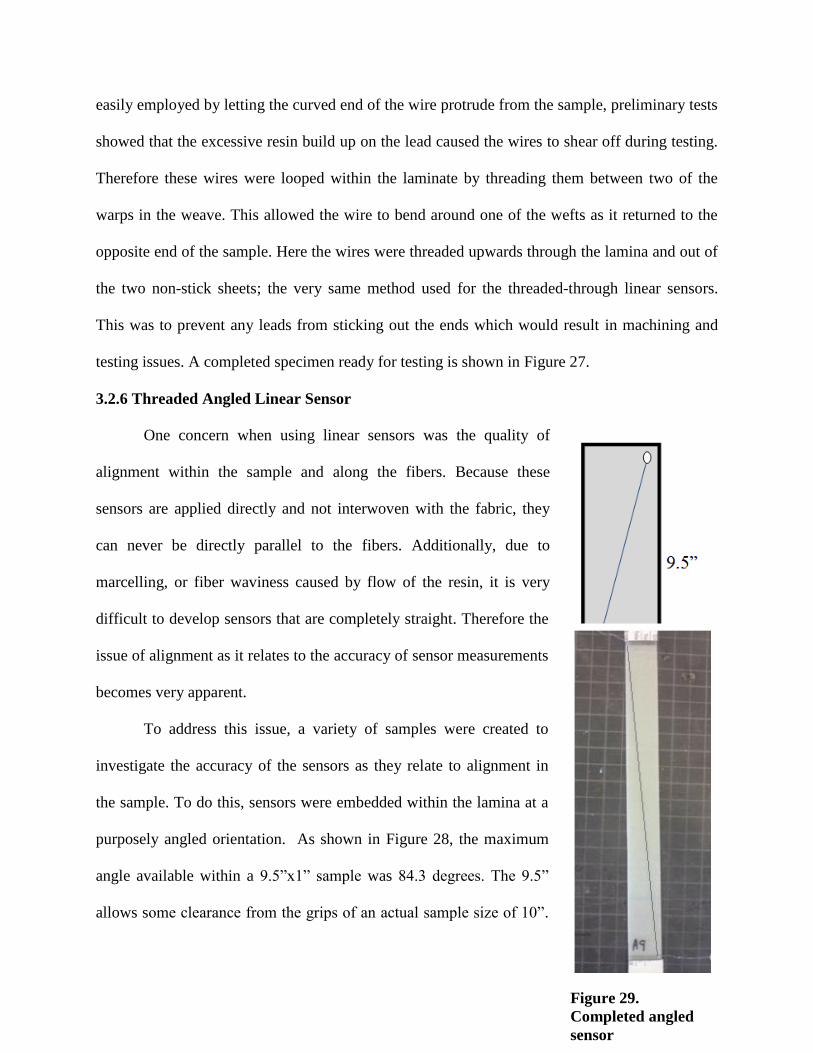
Page | 41
easily employed by letting the curved end of the wire protrude from the sample, preliminary tests
showed that the excessive resin build up on the lead caused the wires to shear off during testing.
Therefore these wires were looped within the laminate by threading them between two of the
warps in the weave. This allowed the wire to bend around one of the wefts as it returned to the
opposite end of the sample. Here the wires were threaded upwards through the lamina and out of
the two non-stick sheets; the very same method used for the threaded-through linear sensors.
This was to prevent any leads from sticking out the ends which would result in machining and
testing issues. A completed specimen ready for testing is shown in Figure 27.
3.2.6 Threaded Angled Linear Sensor
One concern when using linear sensors was the quality of
alignment within the sample and along the fibers. Because these
sensors are applied directly and not interwoven with the fabric, they
can never be directly parallel to the fibers. Additionally, due to
marcelling, or fiber waviness caused by flow of the resin, it is very
difficult to develop sensors that are completely straight. Therefore the
issue of alignment as it relates to the accuracy of sensor measurements
becomes very apparent.
To address this issue, a variety of samples were created to
investigate the accuracy of the sensors as they relate to alignment in
the sample. To do this, sensors were embedded within the lamina at a
purposely angled orientation. As shown in Figure 28, the maximum
angle available within a 9.5”x1” sample was 84.3 degrees. The 9.5”
allows some clearance from the grips of an actual sample size of 10”.
Figure 28.
Threaded angled
linear sensor
orientation within a
single specimen
Figure 29.
Completed angled
sensor

Page | 42
Therefore, the idea can be fabricated with an approximate angle of 84 degrees, or 6 degrees off
perfectly parallel. However, due to tolerances these samples were made with an approximate
angle of 4 degrees off perfectly parallel, measured by a conventional protractor. A completed
specimen is shown in Figure 30. The sensor was difficult to see, so it has been darkened using a
photo editor.
During tensile testing this would cause portions of the cross section to change due to
forces and not due to lengthening of the wire. Additionally, the wire was not perfectly parallel
thus the magnitude of change in length would be less. Therefore, Equation 2 predicts less change
in the measured resistance values. Consequently, the resistance
values from the ohm meter would predict smaller values of ΔR/R
and ΔL/L. The strain would actually be more than the predicted
values. However, investigation of this issue is further discussed in
the experiment sections.
3.2.7 Linear Perpendicular Sensor
To further address concerns of disorientation of the sensor,
an absolute worst case scenario was investigated. A sensor was
embedded in a specimen perpendicular to the direction of applied
force.
This orientation may also glean information on how to detect
strain in the direction perpendicular to any sensor. In this case, the
length was expected to shorten slightly and the cross section should slightly increase. This was
predicted to result in a reduction in resistance values, or a negative trend in the change of
resistance.
Figure 30. Linear
perpendicular sensor
oriented within a
specimen

Page | 43
To simplify fabrication of these samples, they were cleaned up during the layup process
to reduce any need for machining after the cure process. Therefore, each sample was made
individually. A total of five samples for this case were developed.
3.2.8 Full Length Carbon Tow Sensor
Another question to be answered by using this
type of structural health sensing device concerns the
use of constantan. Even though constantan is a widely
used testing material that results in high accuracy of
measurements, it is also fairly expensive and delicate.
Even when compared to carbon, an already fairly
expensive material, constantan is still more precious.
Therefore, it may not be viable for use on a large scale
due to affordability. An alternative is to use other
conductive elements such as Texalium, Celion or
Panex, all conductive yarns.
These substitutes are cheaper
than carbon and still have
conductive properties.
Normally they are made of
fiberglass that has been coated or spun with small bits of aluminum or other conductive metal.
Table 4. T300 6k carbon tow material properties
Material Property
Tensile Strength 545 ksi
Tensile Modulus 33.5 msi
Elongation (%) 1.60
Density 1.78 g/cm3
Resistivity of graphite ~7.837 μΩ-m
Figure 31. T300 6k carbon tow

Page | 44
To investigate the use of other materials and how they can be
employed in this structural health monitoring system, Thornel (owned
by Cytec) T300 6k carbon tow was embedded within the fiberglass
layers. The material properties of the tow are presented in Table 4. A
completed specimen is shown in Figure 32. It was observed that the
elongation for the carbon tow was extremely less than the constantan.
When embedded in the fiberglass it may result in very small changes
in resistance because the elongation was minimal. Additionally, an
average resistivity of carbon (graphite) is presented. This value is far
larger than the resistivity value presented for constantan. Recalling
Equation 2, the changes in length and cross sectional area are
multiplied by the resistivity. Because the resistivity of carbon is larger,
it is expected to experience larger changes in resistance values.
However, coupled with the stiffness and poor elongation of carbon,
this may not be the case. This case was analyzed more in the
experimental results section.
3.2.9 Threaded Through Linear Sensor for Fracture
The last tensile case investigated in support of this study was a fracture case using the
same samples created for studying the effects of the threaded-through linear sensor presented in
Section 3.2.3.
During fracture of the specimen a variety of things can occur. The sensor could fracture
within the fiberglass specimen. The fiberglass could fracture and leave the sensor still intact. Or
they could both fracture simultaneously. The first case was very difficult to measure, because the
Figure 32. Full -
length carbon sensor

Page | 45
Instron machine would not detect any change in structural integrity and would not stop the test.
Thus the only way of measuring the event would be by developing a unique test system or by
eye. More likely one of the two latter cases would occur.
If the sensor fractures the ohm-meter will begin measuring an open circuit and the
resistance will approach infinity. The ohm-meter actually reports a number around 10x1034
when
this happens. Thus, a fracture can be detected by the structural health monitoring device.
If the sensor does not fracture but the fiberglass does, the ohm-meter will not return open
circuit values, but it may exhibit a significant discontinuity in measurements. Thus, specimen
fracture may or may not be detected by the monitoring device.
3.2.10 Threaded Linear Sensor for Flexural
Another objective of this
study was to determine the
sensitivity and feasibility for the
sensor to detect damage within
the composite layers. One main
type of interlaminar damage is a
delamination. A delamination is
very difficult to test in a plane
stress case where load is applied
in only one dimension. The delamination would have no effect on the sample strength during a
tension test because there are no interlaminar forces being exhibited
Figure 33. Schematic of flexural specimen

Page | 46
To effectively investigate a delamination case, a flexural test was used. When a sample is
in bending it undergoes tension, compression, and vertical shear force simultaneously. Thus, a
delamination has a large effect on these out of plane forces.
The samples developed to support this test are in accordance with ASTM Standard
D7264 Standard Test Method for Flexural Properties of Polymer Matrix Composite Materials.
As such, the standard recommends a thickness of 0.16” and a 32:1 span-to-thickness ratio. The
fiberglass layers used in this study are approximately 0.00875” thick. Therefore with 18 layers a
thickness of 0.1575” was achieved and a span of 5.04” was calculated. This specimen width was
0.5”, as recommended by the standard. The recommended dimensions are represented in a
sketch, as shown in Figure 33. A completed specimen is shown in Figure 34.
The sample width was
significantly thin; therefore a linear sensor
was employed. A parabolic sensor could
be used to double the effective sensor
length within the specimen, however, it
was very difficult to manufacture within
the width of the specimens. Unlike the
tensile specimens, there was no
consequence from resin build up on the
leads because there are no clamping jaws
in a bending test. Therefore there was no
risk that the jaws would destroy the leads,
as in the case of the full length linear
Figure 34. (left) Flexural specimen (right)
Delaminated flexural specimen

Page | 47
sensors discussed in Section 3.2.2. Therefore these samples can be machined or cleaned up
during the specimen refining process.
These sensors are embedded between layer 1 and 2 of the 18 layer laminate. This extreme
outer edge will experience the greatest effects of bending due to a greater distance from the
neutral axis. Additionally, this case was tested with the sensors oriented on the upper most
surface of the specimen resulting in compression forces during a 3-point bend test. This was
repeated with the sensors oriented on the bottom most surface, resulting in tension forces. This
method can simultaneously determine the quality of the sensor in a bend test and its ability to
detect compression or tension forces during flexural loads.
3.2.11 Delaminated Threaded Linear Sensor for Flexural
A delaminated case of the threaded linear sensor for flexural testing was developed for
comparison against the previously mentioned non-delaminated case. A 1” delamination was
introduced across the width of the samples. Because the samples are only 5.04” long, this was a
significant delamination. The samples for this case are created in exactly the same way as those
in section 3.2.9. The delamination was introduced between layer 1 and 2 of the laminate; the
same layer that the sensor was embedded within.
Theoretical prediction would estimate that the change in resistance for the delaminated
case would be less than that for the bonded case. Because the sensor was not attached to the
specimen in the delaminated region, it will not experience significant change in length. Therefore
most of the strain in the wire will occur in the remaining 4” of wire length embedded within the
specimen. The 1” difference in strain length can result in variations in resistance measurements,
thus providing a method for detecting delaminations in layers adjacent to the sensor.

Page | 48
3.3 SPECIMEN PREPARATION
3.3.1 Cure Process
Once the fiberglass and sensors are integrated into the middle surface, the plates are
ready to go into the Tetrahedron press for curing. Recall Figure 19 in section 3.1.1, the cure
cycle for the given prepreg material. The cure process takes approximately 90 minutes for the
cure processes and another 30-60 minutes for the plate to cool to room temperature.
3.3.2 Specimen Refinement
Once the plates have been cured in the Tetrahedron press they must be cut down to
standard sizes. ASTM standard D3039 Standard Test Method for Tensile Properties of Polymer
Matrix Composite Materials recommends sample sizes of 10”x1” and 0.1” thick. However, it
must be noted that the actual requirements are more lenient. The standard calls out no required
width or thickness of the specimen. The minimum length must be the gripping length + 2x the
width + gauge length. The specimens made in this study were created from four layers of
fiberglass resulting in a total thickness of 0.035”, thus not the recommended value but still
meeting the requirements. The length used was 9.5” and the width was 1”.
Each case must be refined differently. Because some of the cases result in wire leads out
of the top or bottom of the sample, they could not be
cleaned up without completely cutting through the lead.
Thus, the specimens were cut length-wise only and left as
unrefined along the top and bottom. As mentioned
previously, excessive resin buildup in these areas resulted
in difficulties during testing. This often resulted in the
Figure 35. RIDGID tile saw

Page | 49
clamping jaws destroying the wire leads when put into the Instron machine.
Thus, many of the samples were fabricated in a manner to allow for specimen refinement
and cutting of clean edges. These samples normally had leads that extruded out of the surface of
the specimens, thus allowing the specimen to be cut and squared up.
Using a RIDGID brand tile saw shown in Figure 35, the samples were cut into the sizes
specified by the D3039 standard. The specimens are cut to ±1% of the specimen width in
compliance with the D3039 standard. This means that the specimens are within 0.01” of the 1”
specimen width, or between 0.990” to 1.010”.
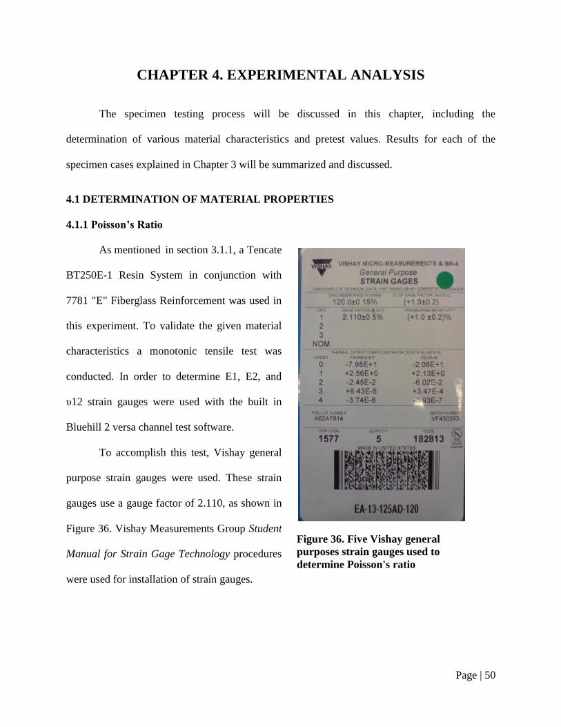
Page | 50
CHAPTER 4. EXPERIMENTAL ANALYSIS
The specimen testing process will be discussed in this chapter, including the
determination of various material characteristics and pretest values. Results for each of the
specimen cases explained in Chapter 3 will be summarized and discussed.
4.1 DETERMINATION OF MATERIAL PROPERTIES
4.1.1 Poisson’s Ratio
As mentioned in section 3.1.1, a Tencate
BT250E-1 Resin System in conjunction with
7781 "E" Fiberglass Reinforcement was used in
this experiment. To validate the given material
characteristics a monotonic tensile test was
conducted. In order to determine E1, E2, and
υ12 strain gauges were used with the built in
Bluehill 2 versa channel test software.
To accomplish this test, Vishay general
purpose strain gauges were used. These strain
gauges use a gauge factor of 2.110, as shown in
Figure 36. Vishay Measurements Group Student
Manual for Strain Gage Technology procedures
were used for installation of strain gauges.
Figure 36. Five Vishay general
purposes strain gauges used to
determine Poisson's ratio

Page | 51
Five specimens were tested in support of
determining material characteristics. The specimen
surface was prepared by surface abrading, degreasing,
applying layout lines, and neutralizing. First, the
specimen was cleaned using acetone. Next the surface
was lightly abraded using 150 grit emery cloth sand
paper. Next, layout lines perpendicular to the
longitudinal length of the specimen were drawn using
pencil. These lines will be used to align the strain
gauge in later steps. Next, using M-Prep Neutralizer,
shown in Figure 37, the surface was neutralized to
provide optimum alkalinity for
adhesives.
Once surface preparation has
been completed, the strain gauges can be
bonded to the specimen. The strain
gauges are extremely small and delicate,
thus should not be handled by hand. The
strain gauges were removed by the
acetate envelope packaging using
tweezers and placed on a clean surface.
Also used are solder terminals, shown in Figure 38, which are used with the strain gauge. These
are placed next to the strain gauge at a 1/6” distance.
Figure 37. A neutralizing agent is
applied to the specimen surface
prior to strain gauges
Figure 38. Bondable terminals are used to
bridge leads to the strain gauges

Page | 52
Using cellophane tape, also called Scotch tape, the strain gauge and terminals were taped
to the clean surface with the soldering surface side upwards, against the tape. Next, the tape was
removed with the strain gauge and terminals attached to the tape. It was then placed on the
specimen in the transverse direction. Using the small alignment triangles on the strain gauges,
the gauge was aligned with the pencil layout lines drawn earlier. Next, the tape was partially
removed allowing the underside to be exposed and looped backwards so that the bottom side of
the strain gauge was exposed. M-Bond 200 catalyst was lightly brushed onto the surface of the
strain gauge, still attached to the tape. M-Bond 200 adhesive was applied to the composite
specimen along the pencil layout line. Next, the tape was repositioned in the original orientation,
along the pencil layout line. Using a piece of thin cotton, the tape was firmly rolled into position,
allowing excess adhesive to move off the side of the specimen. Lastly, firm thumb pressure was
applied for 60 seconds. The tape was removed and the strain gauge was secured firmly in place,
along the layout line, which was along the transverse axis of the specimen. The five specimens
with installed strain gauges are shown in Figure 39. Further details can be found in Vishay
Measurements Group Student Manual for Strain Gage Technology[31]
, presented in the
Appendix.
The Vishay
manual also provides
soldering techniques,
however, these were not
strictly followed. No M-
Coat A was used as called
for in the manual. Solders
Figure 39. Test specimens with installed strain gauges

Page | 53
were made using a generic
soldering iron, shown in Figure
40. The best method found to
solder small terminals such as
those on the strain gauge was to
heat the surface using the
soldering iron and bring the solder
into the region. This quickly melts
the solder and allows it to pool on
the terminal. Once the soldering has melted sufficiently,
the iron can be removed. However, it was important to
be careful as some solder will stick to the iron.
Additionally, it was important to not overheat the
surface and cause the strain gauge to burn out.
Twenty-gauge non-insulated solid copper wires
were bridged between the strain gauge terminals and the
copper solder terminals, as shown in Figure 41.
The copper solder terminals are used to better
connect braided copper lead wire to the strain
gauge. In a similar method as used for soldering
previously, the lead wires were soldered to the
remaining half of the terminals. A completed test
specimen is shown in Figure 42.
Figure 40. Soldering iron used for strain gauge
application
Figure 41. Strain gauge and
terminal bridges applied to test
specimen
Figure 42. Completed test specimen for
Poisson's determination test

Page | 54
To determine Poisson's Ratio, the ASTM standard was used. E132-04 Standard Test
Method for Poisson's Ratio at Room Temperature[32]
outlines the procedure for evaluating data to
determine Poisson's ratio.
The Instron measures extension and true strain directly. Thus to obtain values for
longitudinal strain, no strain gauges were necessary. The longitudinal strain values provided by
the Instron Bluehill 2 software are presented in Figure 43.
Figure 43. Longitudinal strain obtained from Instron using Bluehill software
Values for transverse strain must be obtained by a strain gauge that was aligned with the
lateral direction of the specimen. These values are measured with the versa channel through a
National Instruments BNC-2111 data acquisition box, shown in Figure 44. Values obtained from
0
0.1
0.2
0.3
0.4
0.5
0.6
0.7
0.8
0.9
1
0 200 400 600 800 1000 1200
Str
ain
(%
)
Load (lbf)
Specimen 1
Specimen 2
Specimen 3
Specimen 4
Specimen 5

Page | 55
the strain gauges are presented in Figure 45. Note that the transverse strain is shown as positive
strain. The strain measured is actually negative strain, however, the absolute value has been
taken to represent the data similar to the ASTM standard.
Figure 45. Transverse strain data obtained by Vishay strain gauges
Pursuant to the ASTM standard, the average longitudinal strain
and average transverse strain should be plotted against applied force. It
was important to determine Poisson’s ratio prior to averaging values. Each
calculation was dependent on the sample. If averaging was done at the
strain level, the Poisson’s calculation will be distorted due to deviations
between samples. Thus, it was important to determine either Poisson’s or
-0.02
0
0.02
0.04
0.06
0.08
0.1
0.12
0 200 400 600 800 1000 1200
Str
ain
(%
)
Load (lbf)
Specimen 1
Specimen 2
Specimen 3
Specimen 4
Specimen 5
Figure 44. NI
BNC-2111

Page | 56
strain/load slopes for each case separately and then average them. The slopes of the lines
represent 𝑑𝜖𝑙/𝑑𝑃 and 𝑑𝜖𝑡/𝑑𝑃. The ASTM standard defines Poisson’s ratio as follows:
𝜐 =(𝑑𝜖𝑡/𝑑𝑃)
(𝑑𝜖𝑙/𝑑𝑃)
Equation 7: Poisson’s ratio
Each case is plotted in a manner shown by Figure 46 from ASTM E132-04. Additionally,
the 𝑑𝜖𝑙/𝑑𝑝 and 𝑑𝜖𝑡/𝑑𝑝 slopes for each test specimen are presented in Table 5. With these values
and information, Poisson’s value can be determined for each case. With data for strain in the
longitudinal and lateral directions, in addition to the applied load a plot can be developed per
section 9 of E132-04, presented as Figure 47 on the next page.
Figure 46. Plot of Average strains versus Applied Force for Determination of Poisson’s
Ratio. (Figure 2 from ASTM E132-04)

Page | 57
Table 5. Strain slopes for each specimen case
Sample 1 2 3 4 5 average std dev.
𝑑𝜖𝑙/𝑑𝑝 0.000900 0.000866 0.000923 0.000859 0.000930 0.000896 0.000032
𝑑𝜖𝑡/𝑑𝑝 0.000092 0.000093 0.000091 0.000099 0.000096 0.000094 0.000003
υ 0.102610 0.108364 0.099474 0.116379 0.103998 0.106165 0.006453
Figure 47. Plot of average longitudinal and transverse strains versus applied load
The slope of each line was determined by linear regression using Excel trend-line
function. The slope of the longitudinal strain and transverse strain was determined for each case.
Thus, Poisson’s for each specimen was determined. The average for these five specimens is
presented in Table 5. Therefore the average Poisson's ratio as determined by Equation 6 was
determined to be:
𝜐 = 0.1061 ± 0.008
This value was compared to TenCate test data. TenCate tested a total of five specimens
and determined an average Poisson’s ratio of 0.12. Thus a 12.29% difference was determined.
0
0.1
0.2
0.3
0.4
0.5
0.6
0.7
0.8
0.9
1
0 200 400 600 800 1000 1200
Str
ain
(%
)
Load (lbf)
Transverse Strain
Longitudinal Strain

Page | 58
Note percent difference was used and not percent error. This method is best when neither test
value can be assumed to be absolutely correct.
4.1.2 Weight Fraction
One of the most important factors determining the properties of composites is the
proportions of matrix to reinforcing materials. This is normally presented as a volume fraction,
but, can be also indirectly presented as a weight fraction. The volume and weight fractions are
used exclusively in theoretical analysis of composite materials. Thus it was important to
determine the fraction of the material used for this experiment.
Because volume fraction cannot be determined directly, the weight fraction and density
was measured instead. With these values the volume fraction can be calculated if needed. The
weight fraction is defined as follows:
𝑤𝑐 = 𝑤𝑓 + 𝑤𝑚
𝑊𝑓 =𝑤𝑓
𝑤𝑐 𝑊𝑚 =
𝑤𝑚
𝑤𝑐
Equation 8: Weight fraction
Where c represents composite, f represents fiber, and m represents matrix. A relationship
between volume fraction and weight fraction can be determined by the density of the composite
material. Replacing Equation 8 above using density, it can be rewritten as follows:
𝑊𝑓 =𝑤𝑓
𝑤𝑐=𝜌𝑓𝑣𝑓
𝜌𝑐𝑣𝑐=𝜌𝑓
𝜌𝑐𝑉𝑓
𝑊𝑚 =𝜌𝑓
𝜌𝑐𝑉𝑚
Equation 9: Weight fraction in terms of density
Where 𝑉𝑓 and 𝑉𝑚 are fiber and matrix volume fractions, respectively.

Page | 59
The volume of the fiber and matrix can be calculated by solving Equation 10. Thus the
relations of volume to weight fraction for a composite of two constituents is presented below.[1][2]
𝑉𝑓 =𝜌𝑐𝜌𝑓
𝑊𝑓
𝑉𝑚 =𝜌𝑐𝜌𝑚
𝑊𝑚
Equation 10: Volume fraction
The density of the resin was given by TenCate and presented previously in Section 3.1.1
as 1.17 g/cm3 or 19.17 g/in
3. The fiber density was not provided by TenCate. However, the
composite density can be determined by measuring the dimensions and weight of a sample. Five
samples were measured in support of determining this value. After volume and weight of
composite specimens were measured a burn test was conducted. This was done at approximately
1000°F and 25 minutes per sample until the resin in each specimen was completely burned out.
A summary of results for this test are shown in Table 6. A photo of the burned test specimen
compared to a non-burned test specimen is shown in Figure 48.
Table 6. Summary of weight fraction data
Pre-Burn Post-Burn
Specimen 𝑤𝑐 (g)
𝑉𝑐 (in
3)
Density, 𝜌𝑐
(g/in3)
𝑤𝑓
(g)
𝑤𝑚 (g)
𝑊𝑓 𝑊𝑚
1 2.4 0.076 31.6 1.4 1.0 0.58 0.42
2 2.4 0.077 31.2 1.5 0.9 0.62 0.38
3 2.2 0.075 30.1 1.3 0.9 0.59 0.41
4 2.3 0.073 29.3 1.3 1.0 0.57 0.43
5 2.7 0.087 31.0 1.7 1.0 0.63 0.37
avg 2.4 0.078 30.9 1.44 0.96 0.60 0.40
std dev 0.19 0.01 0.93 0.17 0.05 0.03 0.03

Page | 60
The average weight fraction of the fiber
was calculated to be 0.60. The average weight
fraction of the matrix was calculated to be 0.40.
These were compared to the supplied
manufacturer data of 60 to 70% and 30 to 40%,
fiber and matrix respectively. It can be seen
that the weight fractions are within the range of
specified manufacturer data.
Volume fraction of the fiber can be calculated using the given density of the matrix from
TenCate, measured volume and weight of the composite, and indirect measurement of the fiber
density. Using the average of the five specimens, the volume fraction calculation is shown below
with use of Equation 11.
𝑉𝑓 =
𝑊𝑓𝜌𝑓
𝑊𝑓
𝜌𝑓 + 𝑊𝑚
𝜌𝑚
=0.0325
0.0325 + 0.0286= 0.61
𝑉𝑚 = 1 − 𝑉𝑓 = 0.39
Equation 11: Weight to volume fraction relation
The density of the fiber was not provided directly from TenCate. However, assuming that
the volume does not change between pre- and post-burn, the fiber density can be calculated. This
was a fair assumption, as the composite was not deformed during the burning process. The
matrix was simply being removed, but the fibers retain the same shape.
The volume fraction for the entire composite should be equal to one. Thus the matrix
volume fraction was calculated as shown above. Most pre-pregs are optimized to have a
Figure 48. (left) Burned test sample
compared to (right) unburned sample

Page | 61
maximum volume of fiber and minimum volume of resin. Theoretically, fiber volume fractions
of 90% are predicted; however, actual fiber volume fractions are normally between 70 to 80%.
Comparatively, the experimentally determined volume fractions were 61 and 39%, fiber and
matrix respectively. The values in TenCate’s data sheet are for a fiber volume fraction of 0.60.
Thus, these values are within range by about 1%. The volume fraction plays an important role
for analytical solutions of the composite lamina which is presented in Chapter 5.
4.1.3 Elastic Modulus
In support of determining analytical solutions to validate experimental results, Young’s
modulus was needed. The manufacturer supplied a modulus and ultimate strength, but these were
assumed to be inaccurate. The material used for this project was donated and likely exceeded the
expiration date. Thus, the material properties given by the manufacturer may have changed.
Using ASTM D3039 Standard Test Method for Tensile Properties of Polymer Matrix
Composite Materials, the stress-strain curves were obtained. Specimens were created using the
recommended standards; however, no sensor was inserted into the specimen. Shown in Figure 50
is the stress-strain curve obtained from testing five specimens. Note that specimen number four
fractured significantly before the other specimens. This is acceptable, as only the linear portion
of the curve is needed for determining Young’s modulus. Additionally, the ultimate strength for
the material greatly differs from the manufacturer which was given as 63.0 ksi ultimate tensile
strength.
The first 10% of the data and the last 30% were removed in order to narrow down the
data to the elastic range only, as shown in Figure 49. The first 10% of the data, although in the
elastic range, is not always linear. To determine the slope it is important to obtain a linear
relationship. Additionally the last 30% approaches the plastic range of the material; thus, it is

Page | 62
Figure 50. Stress-strain curve of fiberglass material
-30
-20
-10
0
10
20
30
40
50
0 0.2 0.4 0.6 0.8 1 1.2 1.4 1.6
Str
ess
(ksi
)
Strain (%)
Specimen 1
Specimen 2
Specimen 3
Specimen 4
Specimen 5
Figure 49. Elastic range of stress-strain curve of the fiberglass
0
5
10
15
20
25
30
0 0.1 0.2 0.3 0.4 0.5 0.6 0.7 0.8 0.9 1
Str
ess
(ksi
)
Strain (%)
Specimen 1
Specimen 2
Specimen 3
Specimen 4
Specimen 5

Page | 63
ignored to maintain the linear elastic relationship. The slope of the
elastic range was determined for each case using Excel’s trend-line
function. They were then averaged to obtain the average tensile
modulus for the TenCate 7781 “E” fiberglass BT250E-1 Resin
System material.
Shown in Table 7 are the modulus values for each specimen. The
average Young’s modulus was determined to be 30.119 ksi.
Whereas the manufacturer-supplied modulus was 38.0 ksi. For analytical purposes, the modulus
determined experimentally will be used.
4.1.4 Gauge Factor
The gauge factor of a strain gauge is the ratio of change in electrical resistance to
mechanical strain, as defined in section 2.2. It is an important value that is dependent on the
mechanical properties of the material.
The widely accepted gauge factor for Constantan alloy thin-film strain gauges is
nominally 2. This is a very common value, as most gauge factors for strain gauges range from
about 2 to 2.1. However, the sensor in this study was not specifically a strain gauge; nor was it a
thin film. It will have a significantly different gauge factor. Thus, to investigate the gauge factor
for the material used in this study an experiment was conducted. This value will be determined
independently of values during specimen testing and may assist in predicting strains as they
relate to resistance during the case studies.
Recall Equation 3, the equation for gauge factor of a strain gauge, defined as:
𝐺𝐹 =∆𝑅 𝑅
∆𝐿 𝐿 =
∆𝑅 𝑅
𝜖
Table 7. Summary of
tensile modulus
# E (ksi)
Specimen 1 29.6
Specimen 2 29.191
Specimen 3 30.936
Specimen 4 30.688
Specimen 5 30.182
Average 30.119
std dev 0.729

Page | 64
Therefore, to determine the gauge factor for the wire sensors an experiment was
conducted to measure resistance, change in resistance, and strain. Eight specimens were
fabricated, shown in Figure 51, consisting of solely an 18”
length of wire which was 0.010” in diameter. 1”x1” aluminum
tabs are adhered to each of the wires using 2-part adhesive at a
distance of 9.5” centered about the middle of the constantan
wire. The majority of the laminate samples developed
previously consisted of approximately 9.5” of sensor length
within the specimen and a total length of 18”. Therefore these
lengths are used to mimic values in the case tests.
The sample tabs are placed in the Instron machine and
gripped within the clamping jaws. Knowing the tensile strength
Figure 52. Determination of gauge factor using aluminum tabs
0
0.01
0.02
0.03
0.04
0.05
0.06
0.07
-0.5 0 0.5 1 1.5 2 2.5 3 3.5 4
ΔR
/R
Strain( ΔL/L)
Specimen 1
Specimen 2
Specimen 3
Specimen 4
Figure 51. Wire only
tensile specimen

Page | 65
of constantan to be 455 to 860 MPa (65.992 to 124.723 ksi), as presented in Table 3, some
expectations of testing can be developed. With a wire of cross section 0.010”, the cross sectional
area was calculated to be 7.85x10⁻⁵
in2. Therefore, a tensile force of 5.18 to 9.79 pounds was
expected to result in fracture of the wire. However, the wire exhibits significant elongation.
Therefore the wire will never experience a force over 5 pounds. Instead, it will stretch to nearly
double its length before it fractures.
Knowing this, a test method for tensile testing was developed. The test was set to stop at
an extension of 0.3 inches. This was approximately four times greater than the strain that was
experienced in the specimen case studies. Initial resistance of the wire was measured at points
within the 9.5” length of the wire. Also note that the tabs are aluminum and therefore conductive.
However, they are assumed to experience no strain after the clamping jaws are applied and thus
contribute nothing to the resistance readings during the test. Four samples were tested. During
the test, strain and resistance was measured. Because this test duration was significantly long it
results in over 6000 measurement values. Consequently, a moving average of 50 measurement
samples was used to reduce noise in measurements. From these data, a plot was developed
between the strain and ΔR/R at each point in the test segment. The slope of this line represents
the gauge factor. A trend-line of the data from each test specimen case was developed using
Excel. The slope of the trend-line was recorded as the gauge factor. Various observations can be
made from the plot:
Firstly, Specimen 2 and Specimen 3 are plotted directly on top of each other; next, it is
evident that even though all cases show linear relationships, they do not have the same slope. In
determining the gauge factor, this slope is the most important factor. There are several
explanations for this result. Wires may have small kinks in the length that result in varying

Page | 66
values of strain. The Instron machine is purely metallic, if any wires or leads touch it, it can
interfere with measurements. Also the tabs used to grip the wires may not be ideal; they are
conductive and used adhesive which may not result in sufficient bonding.
Thus, it is apparent that some improvements to this test were necessary. Issues with the
conductive aluminum tabs are the most obvious error. Therefore, the test was recreated using
fiberglass tabs. The fiberglass used was identical to the fiberglass used in the other test cases,
four layers of BT250E-1 TenCate fiberglass.
The test using the fiberglass tabs was repeated using the methods described. The results
for four specimens are shown in Figure 53. Shown are results that are far more consistent. A fair
amount of noise is evident due to the sampling time of the Agilent micro-ohm-meter; however,
this is expected and does not have a large effect on the gauge factor after a linear trend line is
Figure 53. Determination of gauge factor using fiberglass tabs
-0.005000
0.000000
0.005000
0.010000
0.015000
0.020000
0.025000
0 0.1 0.2 0.3 0.4 0.5 0.6 0.7 0.8
ΔR
/ R
Strain (%)
Specimen 1
Specimen 2
Specimen 3
Specimen 4

Page | 67
developed. To develop a single value, the average of the four test specimens was used. The
trend-line slope of the averages is the gauge factor.
Shown in Figure 54 is the average with the linear trend-line. Also shown is the slope of the
line, 0.0296. This value is the gauge factor of the constantan wire.
The gauge factor can provide very good information about the interaction between resistance
and mechanical strain on the wire. However, it is important to note that this value changes when
integrated with other materials. Just like traditional fibrous composites, the fiber and matrix
exhibit individual properties of their own. However, when combined, these properties change
significantly. Thus new mechanical characteristics are needed. This is why many values for
composites are listed in terms of fiber, matrix, and total composite. Similarly for the constantan
wire, its properties change when it was integrated into the fiberglass laminate. It is important to
Figure 54. Average of the gauge factor found when using fiberglass tabs
y = 0.0296x - 0.0011
0.00
0.01
0.01
0.02
0.02
0.03
0.00 0.10 0.20 0.30 0.40 0.50 0.60 0.70 0.80
ΔR
/R
Strain (%)

Page | 68
note this change, as it affects the methods used to predict the strain on the system based on
resistance values.
4.2 TEST DEVICES
Recall Section 2.3 which introduces measurement devices. As mentioned, an Instron
8801 servo-hydraulic system and an Agilent 34420a micro-ohm-meter are used in this study.
Details of how these devices work and how they are used are discussed in this section.
4.2.1 Strain -Stress Test and Measurement Device
The Instron 8801 is an easy to use, precise and
versatile servo-hydraulic testing system. The machine
is shown in Figure 55 with installed 100kN hydraulic
wedge grips. This is the standard setup for most of the
cases in this study.
The software used in conjunction with this
instrument is called Bluehill 2. The data it presents
includes elapsed time, extension (of the lower jaw),
applied load, and strain. The extension is directly
applied to the machine; whereas the applied load is
measured by load cells.
Similarly much of the other information
presented by the interface was calculated indirectly.
The software requires the user to input the dimensions of each sample. This was mainly used to
calculate the stress and strain of the sample. It calculates stress by dividing the applied load at
each time step by the cross sectional area entered by the user. Thus the dimensional measurement
Figure 55. Instron 8801

Page | 69
accuracy of the sample is very important. In addition, the software calculates strain
measurements by dividing the change in extension between two moments in time by the length
entered by the user. Therefore, even though the software provides much data, the data are
actually dependent on one or two variables.
4.2.2 Resistance Measurement Device
The device used to measure
resistance values during this experiment
was an Agilent 34420A 7½ digit, high-
performance nanovolt, micro-ohm meter.
The model has a GPIB (IEEE-488)
interface for data acquisition at 250
samples per second. This device is shown
in Figure 57 along with the 4-wire red
and black terminal leads.
The micro-ohm
meter utilizes the 4-wire
resistance measurement
method to provide accurate
measurements of small
resistances. Test lead
resistance and contact
resistances are
automatically eliminated by
Figure 57. Agilent 34420A micro-ohm-meter
Figure 56. Four-wire measurement method

Page | 70
using this method, thus, the values measured are for the wire sensor alone. Shown in Figure 56 is
the typical configuration of a 4-wire measurement system. The device uses a known current
source and measures the voltage produced by the resistor, thus the resistance can be calculated
indirectly. The micro-ohm meter also comes standard with a GBIP connector which can be used
to record measurements on a computer. This connects directly to a CPU using a USB interface.
To interface with the measurement remotely, a variety of software can be used. The
Agilent hardware supports C++, LabView, and more. In this study, code was developed using
Visual Basic (VBA) through a macro written in Excel. This was the most straight-forward
approach. Often times LabView makes an excellent interface for complicated testing methods;
however, this test was fairly straight-forward and simply measures resistance continually. Thus
the code need only be capable of obtaining resistance values at a sufficient sampling rate.
Setting the sampling rate depends on multiple variables. The ohm-meter has multiple
functions built in and the defaults only allow for a sampling rate of about three measurements per
second. In this test, it was desired to have a sampling rate of approximately ten measurements
per second, as that was the rate the Instron measures. In order to accomplish this, a variety of
variables are changed and the default was not used.
First, the measurement device was set into remote configuration. Next, all commands are
cleared and the meter was reset. The display was then turned off. Using the display uses memory
and reduces the speed of sampling. Additionally, the display does not need to be used because it
does not provide anything valuable when all the measurements are being recorded into an Excel
data sheet. Next, a command was sent to the meter to put it into four-wire resistance
measurement mode. When the meter measures it integrates multiple measurements over a time
period. Increasing this value results in less noise between consecutive measurements and a

Page | 71
higher accuracy; however, it also increases the sampling period. Thus, to increase the sampling
rate the integration time must be reduced. Agilent refers to this integration time as Number of
Power Line Cycles (NPLC). This was set to 0.2, resulting in a maximum of digits shown of 6.5
(micro-ohms) and approximately 16 samples per second. Next, statistics are turned off. This was
more data that the meter was capable of completing, but all the data analysis was completed
separately. Leaving this on just reduces available memory. Lastly, the trigger was set to
immediate with a delay between triggers of zero. This tells the machine to take another
measurement immediately and not use any delay between consecutive measurements. This
completes the remote initialization of the micro-ohm meter; all of the commands can be entered
remotely from a computer. This process only needs to be completed once before each time the
machine was used. The complete VBA code used for this experiment is included in the
Appendix.[27]
Figure 58. Test setup schematic

Page | 72
A schematic of the test setup is presented in Figure 58. A photo of the complete test setup
showing the Instron machine, Agilent micro-ohm-meter, both computers used for data
acquisition and a tensile sample are shown in Figure 59.
Also shown are the four wire leads connected to a tensile specimen current being held in
place by the Instron clamping jaws.
Figure 59. Picture of Test Setup

Page | 73
4.3 TEST SETUP
4.3.1 Tensile Testing Standards
Recall, the tensile test carried out in this experiment was done per ASTM D3039
Standard Test Method for Tensile Properties of Polymer Matrix Composite Materials.[25]
D3039
calls out a few items of note which are important when conducting the experiment.
Material and specimen preparation remains an art rather than a science. The
recommendation provided by the standard states test coupons should be 10” long, 1.0”wide and
0.100” thick. However, the actual requirement states that the length only need be twice the width
+ grip length. Additionally, at least five samples per condition should be tested for statistically
significant data. In this experiment 9.5” was used for the length, 1.0” for width, and 0.035” for
thickness.
Use of tabs was not required. However, one of the standard recommendations is the use
of friction tabs. Friction tabs are essentially non-bonded tabs held in place by the pressure of the
grip often made of emery cloth (80 to 150 grit) or other light abrasive. The tabs used are cut to
1”x2” strips and wrapped completely around the edge of the specimen. They are held onto the
sample by masking tape and further secured by the pressure of the clamping jaws during testing.
Machining methods that are recommended are via the use of diamond tooling that was
water lubricated.
Grip/Tab failures may occur. Failure should not occur within one specimen width of the
tab or grip. Essentially, the failure should occur near the center of the sample and not near the
grips. Prior studies have shown high grip pressure may cause failures near the grips. Thus
reducing the grip pressure will result in acceptable fractures. In this study, only one case of
fracture was investigated.

Page | 74
The majority of the test samples are not tensioned until fracture. In these cases the test
method was set to stop at a 1000 lb. applied load.
4.3.2 Flexural Testing Standards
The flexural testing standards are completed to ASTM D7264 Standard Test Method for
Flexural Properties of Polymer Matrix Composite Materials.[26]
Specifically, this standard points
out recommended dimensions for a test specimen. It is presented in terms of ratios. The standard
span-to-thickness ratio is 32:1, the standard specimen thickness is 0.16 inches, and the standard
specimen width is 0.5 inches, where the length is 20% longer than the support span. Either three-
point or four-point bend can be utilized. For this experiment three-point bend was used because
the specimen was fairly small. It would be difficult to apply two loading points as in four-point
bend.
To accommodate these suggested dimensions, a specimen was made from 18 layers. This
results in a thickness of approximately 0.15 inches. The length of the specimen was 5.04 inches
and the width was 0.5 inches. The sensor was placed between the 1st and 2
nd layer of the
composite specimen.
The support span for testing was set to 3 inches. As the standard recommends a support
span-to-thickness ratio of 20:1, 0.15 inch thickness times twenty was 3 inches.
The load rate was set to 0.05 in/min, as specified by the speed of the testing standard.
Normally this standard is used to test the specimens until fracture. However, the end of test
criteria was a 0.15 inch extension. Thus the test ends before the specimens break. This was
sufficient deflection to obtain valuable data, and the specimen can be reused.

Page | 75
Using this method, the specimens were tested
with the sensor in compression, located on the top of
the beam. Then they were retested with the sensor in
tension, located on the bottom of the beam.
4.4 EXPERIMENTAL RESULTS
Results from the cases discussed in Section 3.2
are presented. Note: the full length linear sensor is not
presented due to the manufacturing difficulties
discussed in Section 3.2.2. Only summaries of the
cases are presented.
4.4.1 Threaded Through Linear Sensor
One of the most basic approaches to integrate
the sensor within the fiberglass laminate was by
making the sensor linear. The difficulty was in
threading the wire through the laminate in the through-
thickness direction. A total of eight specimens were
tested in pure tension and compared to a predicted case
using the gauge factor value determined in Section
4.1.2.
A view of a test specimen within the jaws is
shown in Figure 60. The leads from the four wire
micro-ohm-meter measurement device are connected.
Additionally, a close-up view is shown in Figure 61.
Figure 60. Linear sensor test setup
Figure 61. Close-up of linear
sensor test setup

Page | 76
True strain expressed as a percent was measured using the Bluehill 2 software in
conjunction with the Instron machine. Strain was measured as a function of elapsed time, as
shown in Figure 62. Observe that all the resulting curves are plotted directly on top of each other.
All specimens were made from the same material. Thus, it was expected that they all display the
same strain properties.
Figure 62. Threaded through linear sensor, strain as a function of elapsed time
Similarly, the change in resistance was measured as a function of elapsed time. This was
done independently of the Instron. This would be more representative of a structural health
monitoring system in the field, where it may not rely on interaction with other test equipment.
Shown in Figure 63 on the next page, is the change in resistance per initial resistance values.
-0.2
0
0.2
0.4
0.6
0.8
1
1.2
-20 0 20 40 60 80 100 120 140
Str
ain
(%
)
Elapsed Time (s)
Specimen 1
Specimen 2
Specimen 3
Specimen 4
Specimen 5
Specimen 6
Specimen 7
Specimen 8

Page | 77
Figure 63. Threaded through linear sensor, change of resistance vs. initial resistance
The values presented have been evaluated by a moving average of ten samples. Note that
there is notable noise within the curve. This was due to setting the Agilent micro-ohm-meter
configuration to sample very quickly. This reduces the integration time and does not allow the
machine to average values as it measures. However, this setting was necessary to have sufficient
sampling rates.
An average of the specimens for strain and change in resistance is developed. These
values are plotted against each other in Figure 64. Note that the wavy blue curve represents the
experimental values. The slope of this line represents the gauge factor of the constantan while
embedded within the composite. Recall that the gauge factor for the sensor within the composite
was expected to differ from the gauge factor of the wire on its own. Shown in Figure 64, a gauge
-0.002
0
0.002
0.004
0.006
0.008
0.01
0.012
0.014
0.00 20.00 40.00 60.00 80.00 100.00 120.00 140.00
ΔR
/ R
Elapsed Time (s)
Specimen 1
Specimen 2
Specimen 3
Specimen 4
Specimen 5
Specimen 6
Specimen 7
Specimen 8

Page | 78
factor for the composite system can be developed from the slope. For this case, the gauge factor
was determined to be 0.008445 using Excel’s trend-line fit. Recall that the gauge factor for the
constantan by itself was 0.0294, meaning, the change in resistance for the wire alone was
significantly more than when it was embedded in the composite. This was because the composite
reinforces the sensor and it does not elongate as much.
This value will be used to compare to future experimental cases. As different loading
cases are applied, the strain may become more difficult to predict accurately, as will be discussed
in later sections.
Most importantly, this plot exemplifies strain gauge theory. As strain was applied to the
system the resistance changed. In the case of uni-axial tension, the change was very apparent.
Recall Section 2.2 which introduces the theory of this system. One of the goals of this work was
to develop a system that translates physical strain into electrical measurements and embed the
Figure 64. Threaded through linear sensor, change in resistance vs. strain
y = 0.0084x + 5E-05
0
0.001
0.002
0.003
0.004
0.005
0.006
0.007
0.008
0.009
-0.2 0 0.2 0.4 0.6 0.8 1
ΔR
/ R
Strain (%)

Page | 79
system into a composite laminate. The results of this case prove this relationship to exist within
the developed laminate system. Next, the effectiveness of this relationship will be further
investigated.
4.4.2 Threaded Through Delaminated Sensor
Another goal of this study was to investigate the effectiveness of the structural health
monitoring device to detect delaminations within a composite laminate. One method of doing
this was to test the sensitivity of the sensor to a delamination purposely embedded in the
laminate during an in-plane tension test. Using the specimens fabricated in Section 3.1.2 and
3.2.4, the same test was carried out as described in Section 4.4.1. The data for the change in
resistance as a function of strain is shown in Figure 65. The equation obtained was 0.008504x +
0.000125, as shown on the plot for the delaminated case. A prediction model, obtained from the
gauge factor of the previous test is also plotted. This gauge factor is the gauge factor for the
sensor while in the composite.
Figure 65. Threaded through delaminated case, change in resistance vs. strain
y = 0.008504x + 0.000125
0
0.001
0.002
0.003
0.004
0.005
0.006
0.007
0.008
0.009
0 0.2 0.4 0.6 0.8 1
ΔR
/ R
Strain (%)
Measured (With Delam)
Predicted (Without Delam)

Page | 80
The results from the delam and no-delam cases were compared using percent difference.
Meaning the difference between predicted and measured is divided by the average of the two.
This method is best when neither solution can be assumed to be ideal. Shown in Figure 66, is the
percent difference plotted as a function of strain on the specimen. Note that the percent
difference is relatively high at very low strain values. This was due to the fact that the change in
resistance measurements is on the order of 10-7
. Thus, even an extremely small change in
resistance can have a fairly large effect. This effect could be improved by forcing the change in
resistance to be larger or having a measurement device with more accuracy. One way to make
the change in resistance larger is to use different materials or a material of different size. As there
is more material, there will be more length and thus greater change in overall resistance. The
total average percent difference was 7.06%.
Figure 66. Percent difference between delam and no-delam tensile cases
0
20
40
60
80
100
120
0 0.1 0.2 0.3 0.4 0.5 0.6 0.7 0.8 0.9 1
Per
cen
t D
iffe
ren
ce (
%)
Strain (%)
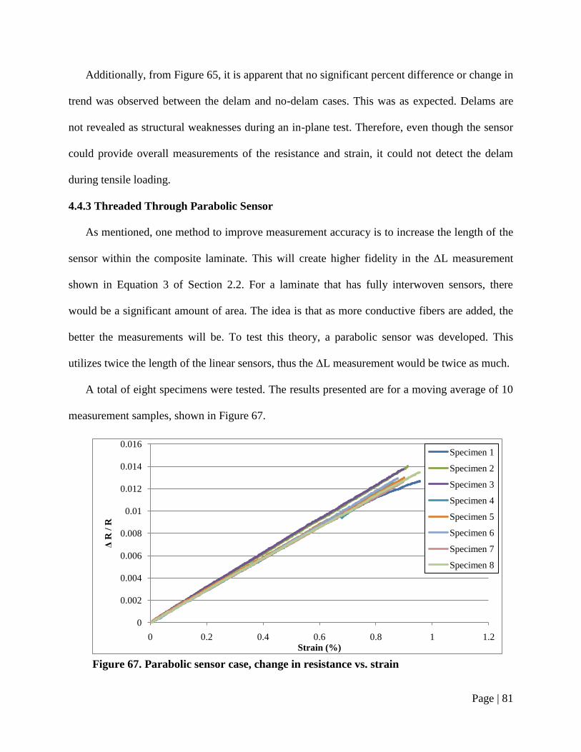
Page | 81
Additionally, from Figure 65, it is apparent that no significant percent difference or change in
trend was observed between the delam and no-delam cases. This was as expected. Delams are
not revealed as structural weaknesses during an in-plane test. Therefore, even though the sensor
could provide overall measurements of the resistance and strain, it could not detect the delam
during tensile loading.
4.4.3 Threaded Through Parabolic Sensor
As mentioned, one method to improve measurement accuracy is to increase the length of the
sensor within the composite laminate. This will create higher fidelity in the ΔL measurement
shown in Equation 3 of Section 2.2. For a laminate that has fully interwoven sensors, there
would be a significant amount of area. The idea is that as more conductive fibers are added, the
better the measurements will be. To test this theory, a parabolic sensor was developed. This
utilizes twice the length of the linear sensors, thus the ΔL measurement would be twice as much.
A total of eight specimens were tested. The results presented are for a moving average of 10
measurement samples, shown in Figure 67.
Figure 67. Parabolic sensor case, change in resistance vs. strain
0
0.002
0.004
0.006
0.008
0.01
0.012
0.014
0.016
0 0.2 0.4 0.6 0.8 1 1.2
ΔR
/ R
Strain (%)
Specimen 1
Specimen 2
Specimen 3
Specimen 4
Specimen 5
Specimen 6
Specimen 7
Specimen 8
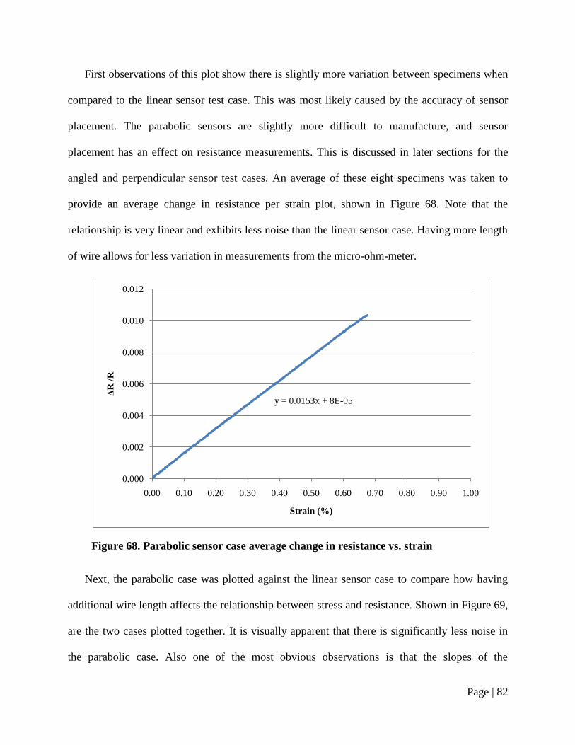
Page | 82
First observations of this plot show there is slightly more variation between specimens when
compared to the linear sensor test case. This was most likely caused by the accuracy of sensor
placement. The parabolic sensors are slightly more difficult to manufacture, and sensor
placement has an effect on resistance measurements. This is discussed in later sections for the
angled and perpendicular sensor test cases. An average of these eight specimens was taken to
provide an average change in resistance per strain plot, shown in Figure 68. Note that the
relationship is very linear and exhibits less noise than the linear sensor case. Having more length
of wire allows for less variation in measurements from the micro-ohm-meter.
Next, the parabolic case was plotted against the linear sensor case to compare how having
additional wire length affects the relationship between stress and resistance. Shown in Figure 69,
are the two cases plotted together. It is visually apparent that there is significantly less noise in
the parabolic case. Also one of the most obvious observations is that the slopes of the
Figure 68. Parabolic sensor case average change in resistance vs. strain
y = 0.0153x + 8E-05
0.000
0.002
0.004
0.006
0.008
0.010
0.012
0.00 0.10 0.20 0.30 0.40 0.50 0.60 0.70 0.80 0.90 1.00
ΔR
/R
Strain (%)

Page | 83
relationship are not the same. In fact, the slope of the parabolic sensor is more similar to the
gauge factor of the wire only test case, completed in Section 4.1.2.
The slope, or gauge factor value, obtained in the parabolic test case was determined to be
0.0153. This differs from the linear sensor value of 0.008445, but relates more closely to the
gauge factor test of 0.0294. Thus, as more sensor length was added the gauge factor of the
composite begins to appear more similar to the gauge factor of the wire.
In a case that has excessively more sensor length, the curve is expected to contain even less
noise. Additionally, the slope would be more consistent between test cases, as there would be a
larger change in resistance being measured. This would also allow for less accurate measurement
devices and thus less expensive equipment.
Figure 69. Parabolic vs. linear sensor change in resistance vs. strain
0.000
0.002
0.004
0.006
0.008
0.010
0.012
0.00 0.20 0.40 0.60 0.80 1.00
ΔR
/ R
Strain (%)
Parabolic
Linear

Page | 84
4.4.4 Threaded Angled Linear Sensor
To test the variation in measurements as it relates to the alignment of the sensor within the
composite laminate, an angled test case was developed. The angled sensor was tested following
the same testing procedures as those for the linear sensor. The only difference was that the
angled sensor has an approximately 6-degree angle within the width of the specimen.
As the sensors that are integrated in this manner cannot always be assumed to be perfectly
straight and along the fiber direction, this test case was done to examine what the consequences
of misalignment are. The test case was compared to the linear sensor case, which was assumed to
be aligned along the fiber direction and in complete tension.
In the angled case, the entire length of the wire was not being taken advantage of. Although
there was slightly more wire within the composite laminate because it was at an angle, the load
was not stretching the wire in the longitudinal direction. Thus some lateral expansion will occur
in the wire while simultaneously the change in length causes the lateral dimension to compress,
thereby having a canceling effect.
To investigate these outcomes, a plot was developed as shown in Figure 70. It represents the
change in resistance per strain for the eight specimens tested. The consistency between test cases
was less than that for the linear cases, which is evident in the plot. This was mostly attributed to
the fact that the angled sensors are more difficult to angle consistently. When the resin flows it
can alter the angle of the sensor somewhat. In case of the linear sensor, tension can be applied so
that the resin flow does not affect the alignment of the sensor. Additionally, the resistance
measurements exhibit far more noise. This was because the stretching that occurs in the
longitudinal direction of the wire, which was not the same as that of the composite, which was
consistently linear. It undergoes longitudinal and lateral tension at the same time.

Page | 85
Next, the average of these eight test specimens was developed and plotted in Figure 71.
Figure 71. Angled sensor, average of change in resistance vs. strain
y = 0.0196x + 0.0004
0
0.002
0.004
0.006
0.008
0.01
0.012
0.014
0.00 0.10 0.20 0.30 0.40 0.50 0.60 0.70
ΔR
/ R
Strain (%)
Figure 70. Angled sensor, change in resistance vs. strain
0
0.002
0.004
0.006
0.008
0.01
0.012
0.014
0.016
0.018
0.00 0.20 0.40 0.60 0.80 1.00
ΔR
/ R
Strain (%)
Specimen 1
Specimen 2
Specimen 3
Specimen 4
Specimen 5
Specimen 6
Specimen 7
Specimen 8
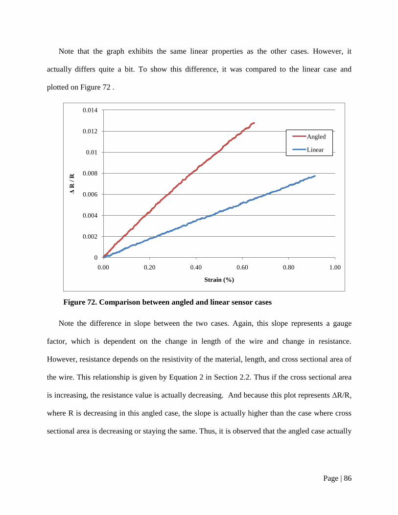
Page | 86
Note that the graph exhibits the same linear properties as the other cases. However, it
actually differs quite a bit. To show this difference, it was compared to the linear case and
plotted on Figure 72 .
Note the difference in slope between the two cases. Again, this slope represents a gauge
factor, which is dependent on the change in length of the wire and change in resistance.
However, resistance depends on the resistivity of the material, length, and cross sectional area of
the wire. This relationship is given by Equation 2 in Section 2.2. Thus if the cross sectional area
is increasing, the resistance value is actually decreasing. And because this plot represents ΔR/R,
where R is decreasing in this angled case, the slope is actually higher than the case where cross
sectional area is decreasing or staying the same. Thus, it is observed that the angled case actually
Figure 72. Comparison between angled and linear sensor cases
0
0.002
0.004
0.006
0.008
0.01
0.012
0.014
0.00 0.20 0.40 0.60 0.80 1.00
ΔR
/ R
Strain (%)
Angled
Linear

Page | 87
results in a steeper slope. The slope was determined via a trend-line to be 0.0196, nearly 2.3
times greater than the slope of the completely linear case.
The observation shows that if the angle of the sensor is off, it will underestimate the
strain on the system for any measured resistance value. This underestimation and error increases
as the strain on the system increases. However, if the angle is known, the gauge factor could be
adjusted to compensate for the underestimation.
Recalling, however, that the intention of this system was to detect changes from baseline
resistance or significant discontinuities in measurements, if a case exists where the sensor was
indeed angled poorly it would not affect a deviation measurement based on baseline
measurements. Because a measurement is always being compared to the initial measurements,
the system will still note a change in strain. However, what will become a problem is the
accuracy of the strain measured. Thus the system may detect an issue, but will not properly
assess the severity.
4.4.5 Linear Perpendicular Sensor
Consider the extreme case of the angled sensor being completely perpendicular to the
direction of loading. This would be an absolute worst case for sensor positioning. However, it
was important to discover how this type of loading may affect sensor measurements. In the case
of this system being used in a real application, there will likely be many times when loading will
not be as ideal as can be created in the lab. Five samples were created to test this scenario, shown
in Figure 73 is the change in resistance response for each case.
Note the extreme noise in the plot. This noise was exaggerated because of the very small
values of ΔR/R. In reality it was not much more than any of the other cases shown previously.
However, note that the trends are not linear. The measurements fluctuate around zero. Specimens

Page | 88
4 and 5 have a slight negative trend which may be due to a perfectly perpendicular sensor or
abnormalities in the deformation due to how the composite was laid up.
To glean a little more understanding of these effects, the average of all these cases was
plotted in Figure 74. Additionally, the total average of the cases was plotted as a red horizontal
line on the graph. This represents the value about which most of the readings are fluctuating. It is
0.00166 away from a change in resistance of zero. What is most evident about these results is
that no apparent trend is observed. Thus, sensors oriented perpendicular to the load direction of
the specimen provides no useful feedback. These readings are similar to what would occur if no
load was applied, as even static loads exhibit significant fluctuation. From this test it can be
deduced that sensors oriented in different directions will measure strain independently of each
Figure 73. Perpendicular sensor, change in resistance vs. strain
-0.012
-0.01
-0.008
-0.006
-0.004
-0.002
0
0.002
0.004
0.006
0 0.1 0.2 0.3 0.4 0.5 0.6 0.7 0.8 0.9
ΔR
/R
Strain (%)
Specimen 1
Specimen 2
Specimen 3
Specimen 4
Specimen 5

Page | 89
other. Thus, if multiple sensors are to be used in an application it can be easily determined in
which direction the part is being loaded.
This test case shows that when the specimen was loaded perpendicular to the sensor
orientation, there was little effect on the resistance measured by the micro-ohm-meter.
Additionally, it shows that very little information can be determined from measurements of this
type. If this were a measurement in an application study, it would be difficult to understand the
effects of loading directly from the resistance plots.
4.4.6 Full Length Carbon Tow Sensor
Although very good at providing accurate and consistent results, constantan wire was fairly
difficult to work with and was quite expensive. It is actually more expensive than carbon fiber
tow. However, constantan retains the benefits of low resistance, minor temperature dependence,
Figure 74. Average of perpendicular sensor case
-0.004
-0.0035
-0.003
-0.0025
-0.002
-0.0015
-0.001
-0.0005
0
0.0005
-0.1 0 0.1 0.2 0.3 0.4 0.5 0.6 0.7
ΔR
/R
Strain (%)

Page | 90
and high elongation, and thus it is very sensitive to measurements. However, many other
materials can be used that may improve ease of embedding the sensor in the laminate. The
system should be easy to use with little effort needed to perfect the sensors. Therefore, other
avenues were explored.
Carbon fiber is already widely used for its high stiffness properties. However, an under-
utilized property of carbon fiber is its conductive properties. Although very strong, it is very
capable of carrying a current. Additionally, when compared to constantan it is more readily
available, comes in many different forms and is less expensive. The disadvantages are that it will
likely not be very sensitive to measurements because of its high stiffness and low elongation
properties. To combat this, there are many other materials that could be used such as Texalium.
Texalium is one form of a fiberglass that has aluminum fibers intertwined with each fiber of the
glass, thus creating a fiberglass that is actually conductive. There are many more examples of
this which utilize other materials.
To study how carbon fiber might be used as a sensor, it was embedded within the fiberglass
laminate in a similar fashion as the constantan wire. However, unlike the other cases, it was not
threaded through the laminate in the through-thickness direction. Instead, it was fabricated by
allowing the end to protrude out of the end of the laminate. When constantan was constructed
this way it caused problems because the leads would break off. However, carbon is must stiffer
than the constantan and less prone to breaking.
Using these samples, the same test procedure for the linear sensor was carried out. The
results are shown in Figure 75.
Note that the linear trends that are representative of tension were similar for the previous
cases. However, also note the inaccuracy of measurements. This was because carbon was so stiff

Page | 91
that it does not begin to strain until higher loads are applied. Thus the fiberglass has already
begun to deform and the carbon had not been able to detect these strains. It was also not as
consistent under loading conditions because the sensor was now fibrous and not solid. However,
for an application case, theses strains may be sufficient. Even though the carbon sensors result in
inaccurate results, they may still be used to determine structural integrity; however, their use
should definitely be improved upon for reliability.
The average of the samples was taken and plotted in Figure 76. The plot is very similar to
that of previous averaged cases.
Figure 75. Carbon sensor, change in resistance vs. strain
0
0.002
0.004
0.006
0.008
0.01
0.012
0.014
0.016
0.018
0 0.2 0.4 0.6 0.8 1
ΔR
/R
Strain (%)
Specimen 1
Specimen 2
Specimen 3
Specimen 4
Specimen 5
Specimen 6
Specimen 7
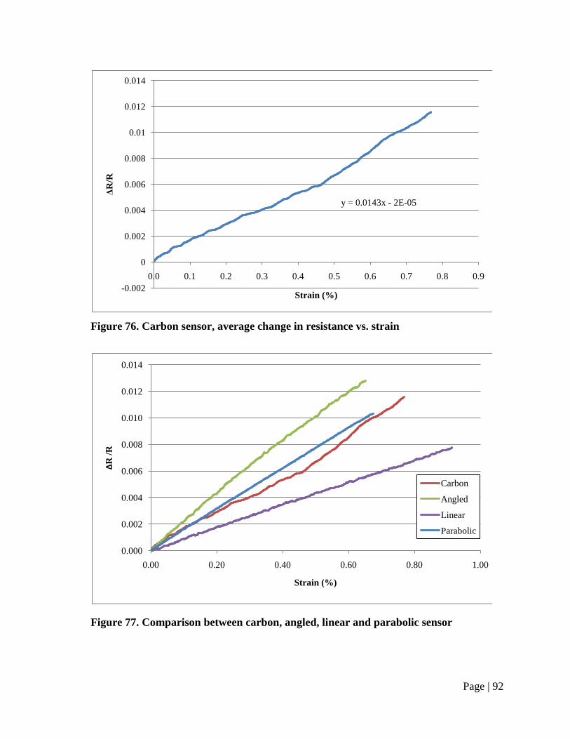
Page | 92
Figure 77. Comparison between carbon, angled, linear and parabolic sensor
0.000
0.002
0.004
0.006
0.008
0.010
0.012
0.014
0.00 0.20 0.40 0.60 0.80 1.00
ΔR
/R
Strain (%)
Carbon
Angled
Linear
Parabolic
Figure 76. Carbon sensor, average change in resistance vs. strain
y = 0.0143x - 2E-05
-0.002
0
0.002
0.004
0.006
0.008
0.01
0.012
0.014
0.0 0.1 0.2 0.3 0.4 0.5 0.6 0.7 0.8 0.9
ΔR
/R
Strain (%)

Page | 93
Additionally, the values were compared to the parabolic and linear sensor cases, shown in
Figure 77. A difference in slope was expected, as this was a sensor that was completely different
than the constantan. However, noting that the same trend was followed is important. Again,
because the system can be used to measure deviations from initial measurements, the carbon
sensor can be used in much the same way constantan can. However, because of its properties it
may have a different reaction to continued fatigue or thermal properties. In any case this test
shows that common carbon tows could be utilized as a sensor. Therefore many existing and
newly fabricated parts could integrate a sensor without changing the material being used to
fabricate it.
4.4.7 Threaded Through Linear Sensor for Fracture
Consider the scenario where the specimen is not simply experiencing strain then elastically
returned to its original shape, but where fracture actually occurs and the specimen breaks. In this
case there are a couple of possible outcomes for how the micro-ohm-meter might determine the
current health of the structure.
During a fracture the fiberglass specimen will break, however, the sensor within the
composite may or may not break. If it does completely fracture with the fiberglass the circuit will
become open and the resistance readings will approach infinity. In this case the ohm-meter
returns an extremely large resistance reading. Another possible outcome is that the fiberglass
snaps in an area that exposes the wire, but it remains intact. During the fracture the stress will be
relieved. Thus the strain will be as well, and the resistance measurements will return to a nominal
value around where the readings started. However, due to plasticity the values may not return to
exactly the same value. The last case was when the fracture was localized in an area that does not
cause the sensor to become exposed or damaged in any way. In the case where the wire was
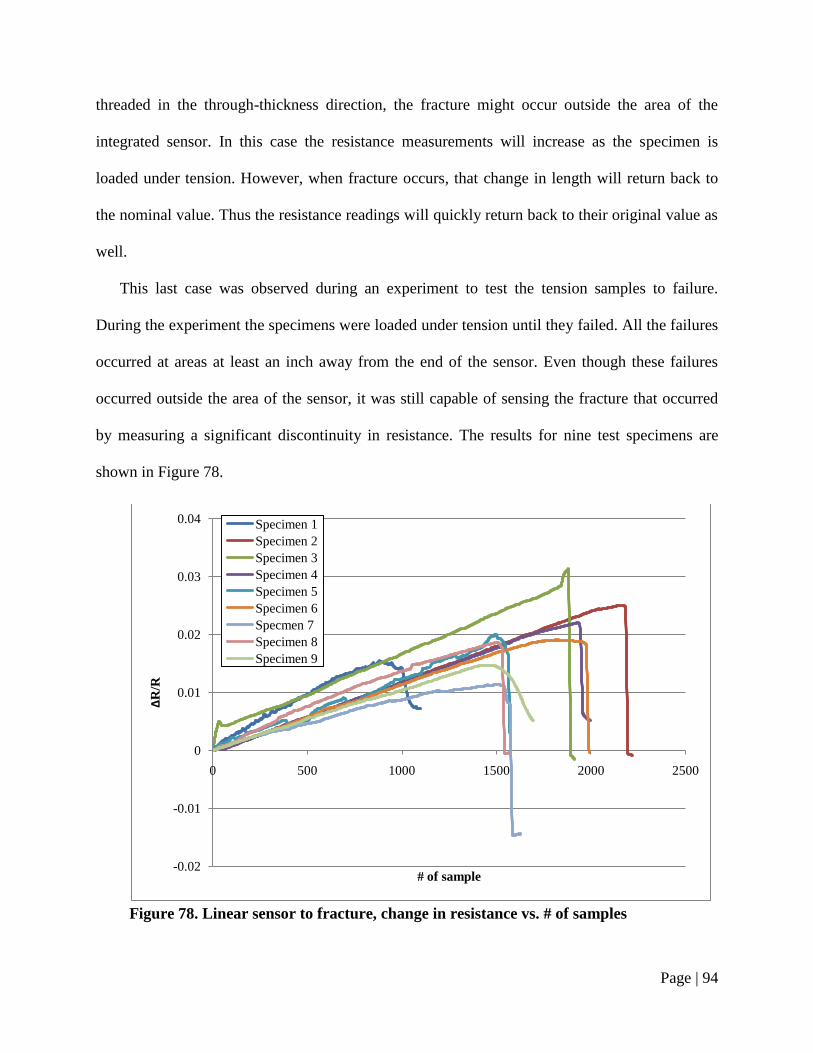
Page | 94
threaded in the through-thickness direction, the fracture might occur outside the area of the
integrated sensor. In this case the resistance measurements will increase as the specimen is
loaded under tension. However, when fracture occurs, that change in length will return back to
the nominal value. Thus the resistance readings will quickly return back to their original value as
well.
This last case was observed during an experiment to test the tension samples to failure.
During the experiment the specimens were loaded under tension until they failed. All the failures
occurred at areas at least an inch away from the end of the sensor. Even though these failures
occurred outside the area of the sensor, it was still capable of sensing the fracture that occurred
by measuring a significant discontinuity in resistance. The results for nine test specimens are
shown in Figure 78.
Figure 78. Linear sensor to fracture, change in resistance vs. # of samples
-0.02
-0.01
0
0.01
0.02
0.03
0.04
0 500 1000 1500 2000 2500
ΔR
/R
# of sample
Specimen 1
Specimen 2
Specimen 3
Specimen 4
Specimen 5
Specimen 6
Specmen 7
Specimen 8
Specimen 9
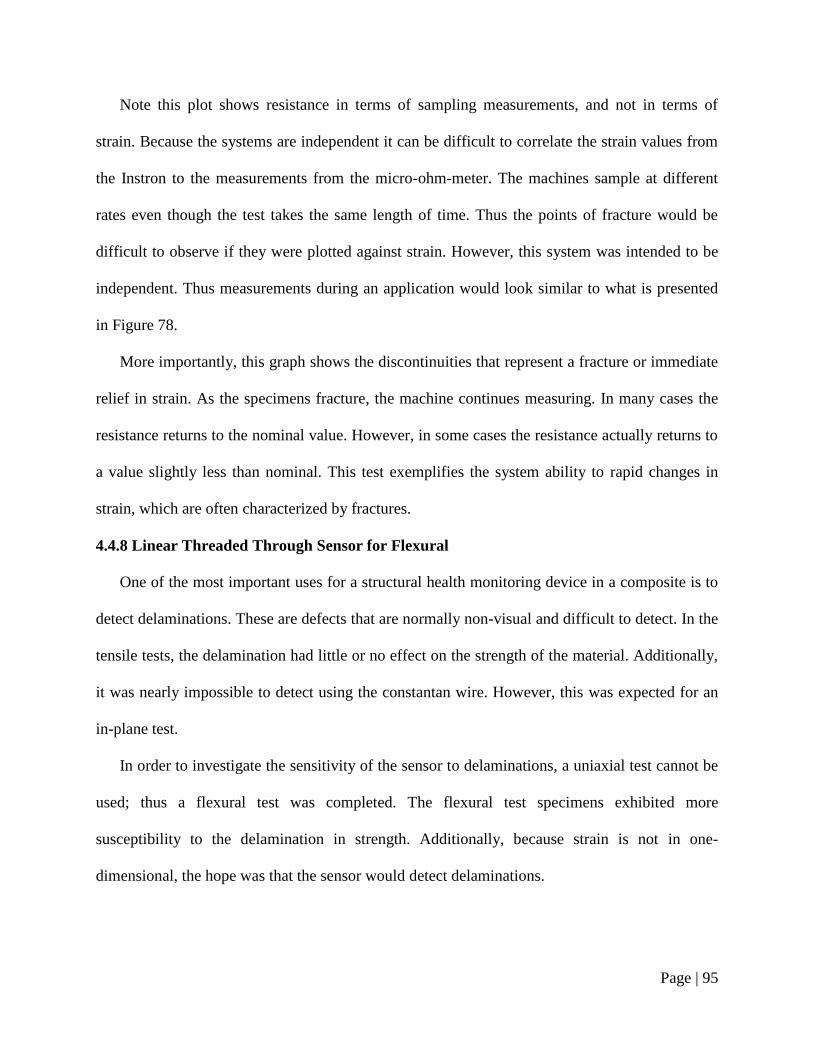
Page | 95
Note this plot shows resistance in terms of sampling measurements, and not in terms of
strain. Because the systems are independent it can be difficult to correlate the strain values from
the Instron to the measurements from the micro-ohm-meter. The machines sample at different
rates even though the test takes the same length of time. Thus the points of fracture would be
difficult to observe if they were plotted against strain. However, this system was intended to be
independent. Thus measurements during an application would look similar to what is presented
in Figure 78.
More importantly, this graph shows the discontinuities that represent a fracture or immediate
relief in strain. As the specimens fracture, the machine continues measuring. In many cases the
resistance returns to the nominal value. However, in some cases the resistance actually returns to
a value slightly less than nominal. This test exemplifies the system ability to rapid changes in
strain, which are often characterized by fractures.
4.4.8 Linear Threaded Through Sensor for Flexural
One of the most important uses for a structural health monitoring device in a composite is to
detect delaminations. These are defects that are normally non-visual and difficult to detect. In the
tensile tests, the delamination had little or no effect on the strength of the material. Additionally,
it was nearly impossible to detect using the constantan wire. However, this was expected for an
in-plane test.
In order to investigate the sensitivity of the sensor to delaminations, a uniaxial test cannot be
used; thus a flexural test was completed. The flexural test specimens exhibited more
susceptibility to the delamination in strength. Additionally, because strain is not in one-
dimensional, the hope was that the sensor would detect delaminations.

Page | 96
First a case with no delamination was completed. This will be used to compare to the
delaminated case in the next Section. Four cases were tested with the sensor along the top
surface, putting it into compression. The test was then repeated with the sensor along the bottom,
in tension.
The test specimen under load is shown in Figure 79. The ohm-meter leads are connected to
the sensor protruding from the ends of the beam.
The results from the compression case for all four specimens are presented in Figure 80.
Specimen 1 exhibited more noise in measurements than the other specimens. This was likely due
to electrical interference. All the test equipment was metallic and it was very difficult to insulate
the test. This noise was discovered in other trials where contacts with test equipment were made.
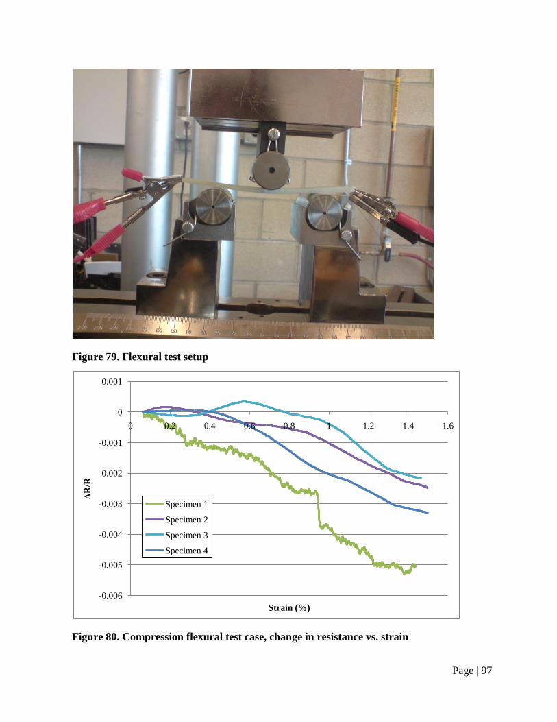
Page | 97
Figure 80. Compression flexural test case, change in resistance vs. strain
-0.006
-0.005
-0.004
-0.003
-0.002
-0.001
0
0.001
0 0.2 0.4 0.6 0.8 1 1.2 1.4 1.6
ΔR
/R
Strain (%)
Specimen 1
Specimen 2
Specimen 3
Specimen 4
Figure 79. Flexural test setup

Page | 98
As expected, the trend shown is negative for all cases. A negative change in resistance
correlates to a compression force on the upper surface of the bending specimen. The variation in
results was likely due to a difference in specimen dimensions. The heated press was not very
good at making consistent thicknesses when working with material 18-layers thick. This was
simply a limitation of the lab equipment. If the specimens were created under better tolerances,
the plot would likely have less variation. However, this would require better lab equipment.
The average of these measurements was taken at each strain value and shown in Figure 81.
Next, consider the case where the sensor was located along the bottom of the beam. Here the
sensor will experience tension.
Figure 81. Average of flexural bending test under compression
-0.0035
-0.003
-0.0025
-0.002
-0.0015
-0.001
-0.0005
0
0.0005
0 0.2 0.4 0.6 0.8 1 1.2 1.4 1.6
ΔR
/R
Strain (%)

Page | 99
Note the positive trend. This was evidence of the tensile forces that the bending specimens
are experiencing. Specimen 1 shows a slightly different trend, but still following a positive trend.
The samples are a little more consistent than in the compression test.
The average of these test cases is plotted in Figure 83. It shows a similar trend to that of the
compression case, but in the opposite direction.
Figure 82. Tensile flexural test case, change in resistance vs. strain
-0.001
0
0.001
0.002
0.003
0.004
0.005
0.006
0.007
0.008
0 0.2 0.4 0.6 0.8 1 1.2 1.4 1.6
ΔR
/R
Strain (%)
Specimen 1
Specimen 2
Specimen 3
Specimen 4

Page | 100
The test cases show that the sensor was capable of detecting strain on the specimen under
flexural loads. More importantly it was easy to determine the difference between tensile and
compression loads. The accuracy of the measurements was more difficult to determine. The
system provides a fair amount of noise between measurements at its current settings. However,
more important is the system’s ability to measure deviations from baseline measurements and to
determine deviations from ideal structural health. One deviation from ideal structural health
would be a delamination within the composite laminate. This case is discussed in the next
Section.
4.4.9 Delaminated Linear Threaded Through Sensor for Flexural
Detecting delaminations in the composite laminates is essential for determining the structural
health of the specimen. Normally, delaminations are nearly impossible to detect. With the aid of
non-destructive test equipment such as ultrasound or x-ray, they can sometimes be detected.
However, this requires considerable equipment, time and trained personnel.
Figure 83. Average of flexural bending test under tension
-0.001
0
0.001
0.002
0.003
0.004
0.005
0.006
0.007
0 0.2 0.4 0.6 0.8 1 1.2 1.4 1.6
ΔR
/R
Strain (%)

Page | 101
A structural health monitoring system's greatest advantage is that it can provide real time
structural health data to a user at any time with minimum equipment and personnel. Thus to
further validate the use of embedded sensors for the use of structural health monitoring in
composite laminates a flexural test was conducted. Unlike the delaminated case under tension,
the flexural test was greatly affected by the existence of a delamination.
The test setup is shown in Figure 84. Note that the delamination was clearly observable.
During compression, the area becomes significantly debonded from the rest of the beam.
The results for four test specimens are plotted in Figure 85
Figure 84. Delaminated flexural test case under compression

Page | 102
Recall Figure 80 for the nondelaminated case. The plots look similar with a overall negative
trend. A comparison will be done later to better understand the similarities and differences.
The average of these data is plotted in Figure 86.
Figure 85. Delaminated compression flexural test case, change in resistance vs.
strain
-0.006
-0.005
-0.004
-0.003
-0.002
-0.001
0
0.001
0.002
0 0.2 0.4 0.6 0.8 1 1.2 1.4 1.6
ΔR
/R
Flexural Strain (%)
Specimen 1
Specimen 2
Specimen 3
Specimen 4

Page | 103
Next, consider the case where the sensor was located along the bottom of the beam and
experiences tension. Shown in Figure 87 are the results for each test case.
Figure 87. Delaminated tension flexural test case, change in resistance vs.
strain
-0.001
0
0.001
0.002
0.003
0.004
0.005
0.006
0.007
0 0.2 0.4 0.6 0.8 1 1.2 1.4 1.6
ΔR
/R
Flexural Strain (%)
Specimen 1
Specimen 2
Specimen 3
Specimen 4
Figure 86. Average of delaminated flexural bending test under compression
-0.004
-0.0035
-0.003
-0.0025
-0.002
-0.0015
-0.001
-0.0005
0
0.0005
0.001
0 0.2 0.4 0.6 0.8 1 1.2 1.4 1.6
ΔR
/R
Flexural Strain (%)

Page | 104
The average of these four specimens was taken and plotted in Figure 88, shown below. Note
that it follows a similar trend as the non-delaminated case.
Again, as expected, a positive trend was observed. One note on the bending cases was that
the trends were not completely linear. This differed from the tensile cases.
Next, a comparison between the delaminated and nondelaminated cases was done. Both the
compression and tension cases were compared. This comparison showed the sensor’s sensitivity
to the delamination and, thus, its ability to detect a delamination while under load. Of course, if
no load was applied, this sensing method would most likely not detect the delamination. The
compression test cases for the delaminated and nondelaminated averages are shown in Figure 89.
Figure 88. Average of delaminated flexural bending test under tension
-0.001
0
0.001
0.002
0.003
0.004
0.005
0.006
0 0.2 0.4 0.6 0.8 1 1.2 1.4 1.6
ΔR
/R
Strain (%)

Page | 105
Observe that the delaminated case has overall a greater value of change of resistance. This
was because the sensor was not bonded within the composite laminate and not constrained to
compress with the composite. Instead, this area does not undergo compression. Therefore, less of
a compression effect was measured. There was a notable difference between the delaminated and
nondelaminated cases. Thus the sensor was capable of differentiating between a delaminated and
nondelaminated test case under certain conditions: the specimen needs to be under load and
needs to be within the layer of delamination.
Next, the tensile case was compared. Shown in Figure 90 are the delaminated and
nondelaminated test case averages.
Figure 89. Comparison between delaminated and nondelaminated flexural cases
under compression
-0.004
-0.0035
-0.003
-0.0025
-0.002
-0.0015
-0.001
-0.0005
0
0.0005
0.001
0 0.2 0.4 0.6 0.8 1 1.2 1.4 1.6
ΔR
/R
Strain (%)
Delamination
No Delamination

Page | 106
Under tension, the sensor in the delaminated case was not being loaded as much as in the
nondelaminated case. Thus, the change of resistance readings is less for all values of strain.
The compression and tension cases both exhibited differences between delaminated and
nondelaminated specimens. This shows that the sensor was capable of detecting structural health
defects in the composite laminate.
4.5 SUMMARY OF EXPERIMENTS
Each test conducted in support of this research has been in support of the development of
a resistance-based sensor to monitor the structural health of a composite laminate. Each test
provided a significant conclusion. These tests and conclusions are summarized in Table 8.
Figure 90. Comparison between delaminated and nondelaminated flexural cases
under tension
-0.001
0
0.001
0.002
0.003
0.004
0.005
0.006
0.007
0 0.2 0.4 0.6 0.8 1 1.2 1.4 1.6
ΔR
/R
Strain (%)
Delamination
No Delamination
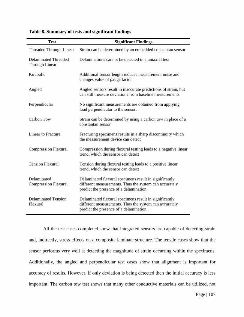
Page | 107
Table 8. Summary of tests and significant findings
Test Significant Findings
Threaded Through Linear Strain can be determined by an embedded constantan sensor
Delaminated Threaded
Through Linear
Delaminations cannot be detected in a uniaxial test
Parabolic Additional sensor length reduces measurement noise and
changes value of gauge factor
Angled Angled sensors result in inaccurate predictions of strain, but
can still measure deviations from baseline measurements
Perpendicular No significant measurements are obtained from applying
load perpendicular to the sensor.
Carbon Tow Strain can be determined by using a carbon tow in place of a
constantan sensor
Linear to Fracture Fracturing specimens results in a sharp discontinuity which
the measurement device can detect
Compression Flexural Compression during flexural testing leads to a negative linear
trend, which the sensor can detect
Tension Flexural Tension during flexural testing leads to a positive linear
trend, which the sensor can detect
Delaminated
Compression Flexural
Delaminated flexural specimens result in significantly
different measurements. Thus the system can accurately
predict the presence of a delamination.
Delaminated Tension
Flexural
Delaminated flexural specimens result in significantly
different measurements. Thus the system can accurately
predict the presence of a delamination.
All the test cases completed show that integrated sensors are capable of detecting strain
and, indirectly, stress effects on a composite laminate structure. The tensile cases show that the
sensor performs very well at detecting the magnitude of strain occurring within the specimens.
Additionally, the angled and perpendicular test cases show that alignment is important for
accuracy of results. However, if only deviation is being detected then the initial accuracy is less
important. The carbon tow test shows that many other conductive materials can be utilized, not

Page | 108
just constantan. In fact, carbon would make a great sensor because it is already widely used for a
large variety of parts. The discontinuities discovered under testing the fracture cases show that
the sensor is capable of detecting rapid changes in strain. Additionally, the bending cases show
that the sensor is capable of not only detecting flexural strain, but also differentiating between
delaminations for compressive and tensile loads. These tests provide a foundation for a better
integrated sensor. They prove that this method works, but inherent challenges are also present.
By developing a more careful integration process, having a greater length of sensor, or better
alignment and layup techniques this method can easily be implemented in the many new
structural parts with little cost. This would allow composite parts to be monitored at any given
time for their structural health; thus providing essential information to engineers and
maintenance to resolve issues before catastrophic damage is done.

Page | 109
CHAPTER 5. THEORETICAL ANALYSIS
Analytical solutions of select test cases are developed for comparison to experimental
values. The solutions are used to validate the experimental measurements and show the results
are as expected. Strain was predicted for comparison to the experimental values measured by the
Instron machine. Resistance was predicted for comparison to the experimental values measured
by the Agilent micro-ohm-meter.
5.1 STRAIN PREDICTION
For a composite laminate under load in a single direction, the stress-strain relationship in
the same direction is simplified to Hooke’s Law, shown in Equation 12.
𝜎 = 𝐸 ∗ 𝜖
Equation 12: Hooke’s Law
Young’s modulus was determined to be to be 30.119 ksi from Section 4.1.3. Also, the
relationship σ=F/A can be used. The normal force ranges from 0 to 1000 pounds, and the area of
each specimen was calculated from the width times thickness. Using the full length linear sensor
case as an example, an analytical solution can be developed. Strain was calculated for each
specimen for a range of forces. The average was then taken and plotted, as shown in Figure 91.
Also plotted is a comparison to the average of the experimental measurements for the full length
linear sensor. Good agreement is observed between the two cases. The experimental values show
deviation from the linear relationship; whereas the theoretical solution remains linear for all
loads.
The percent difference between the two cases was calculated and plotted as shown in
Figure 92. The difference is larger at low values of applied force because the values being
compared are extremely small. However, error converges to about 11% and higher loads.

Page | 110
Figure 92. Percent difference between experimental and theoretical strain solutions
for full length linear test case
0
2
4
6
8
10
12
14
16
18
0 200 400 600 800 1000 1200
Dif
feren
ce (
%)
Load (lbs)
Figure 91. Comparison between experimental and theoretical strain solutions for full
length linear sensor test case
0
0.2
0.4
0.6
0.8
1
1.2
0 200 400 600 800 1000 1200
Str
ain
(%
)
Load (lbs)
Experimental
Theoretical

Page | 111
The analytical solution shows that experimentally obtained values are in agreement with
expected values. Thus, the strains of the fiberglass specimens obtained by the Instron machine
are within approximately 11% of an ideal test case.
5.2 RESISTANCE PREDICTION
Another important validation was the resistance measurements made by the Agilent
micro-ohm-meter. These values can be obtained by directly correlating the strain to resistance by
the gauge factor. However, results show the gauge factor to differ significantly due to length and
orientation. Thus, resistance was validated using the material constant of resistivity. For
constantan the resistivity is 1.925x10⁻⁵
ohm-inch. Recall Equation 2 for determining resistance of
a wire based on resistivity.
R = ρl
A
Resistivity, ρ, is a known material property. Additionally the cross section area, A, is
known, as the diameter of the wire used was 0.010 inches. The initial length, l, is known. This
value changes as load is applied to the specimen. However, this change is dependent on the
extension of the Instron machine. Thus resistance can be measured at every point during testing
based on the change in length of the specimen.
Using these methods, a theoretical model can be developed. Shown in Figure 93, is the
theoretical model plotted against the measured experimental values. Similar to the prediction for
strain which over predicted strain values; the theoretical resistance model obtained larger values
of resistance. Also, the experimental values again stray from an ideal linear case.
The percent error between the theoretical and experimental cases is plotted in Figure 94.
Note, percent error is used for this analysis as the theoretical solution is assumed to be ideal.
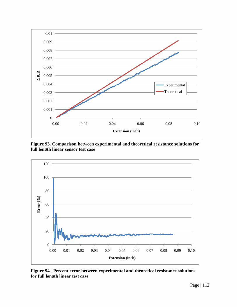
Page | 112
Figure 94. Percent error between experimental and theoretical resistance solutions
for full length linear test case
0
20
40
60
80
100
120
0.00 0.01 0.02 0.03 0.04 0.05 0.06 0.07 0.08 0.09 0.10
Err
or
(%)
Extension (inch)
Figure 93. Comparison between experimental and theoretical resistance solutions for
full length linear sensor test case
0
0.001
0.002
0.003
0.004
0.005
0.006
0.007
0.008
0.009
0.01
0.00 0.02 0.04 0.06 0.08 0.10
ΔR
/R
Extension (inch)
Experimental
Theoretical

Page | 113
However, the average percent error was approximately 14%, which relates more closely
to the error obtained during the theoretical and experimental strain comparison. The trend also
assumes that resistivity of the wire was the published value. Variations in alloy elements can
cause this value to change slightly, a better estimate can be obtained by measuring resistivity of
the material directly. Moreover, the analytical solution again shows fairly good agreement with
the experimentally obtained values. Additionally, the error was very similar to the error obtained
in the strain case. The trends are both very similar. Meaning the resistance follows a similar trend
to strain, which was expected.

Page | 114
CHAPTER 6. CONCLUSION AND RECOMMENDATIONS
The goal of this research was to develop a simple method for measuring deviations from
baseline health and identifying potential catastrophic structural failures in a composite laminate
by utilizing an integrated resistance-based monitoring system.
The strain in a fiberglass laminate was determined by using an embedded constantan wire as
a conductive element. With no other tools besides an ohm-meter, the system could predict the
strain and stress on the structure. A variety of orientations were tested to investigate the fidelity
in the measurement sensitivity and necessary placement of the sensor. The orientation had a
significant effect on accuracy of measurement values, but not on deviations from baseline
measurements. Additionally, using a sensor of greater length resulted in higher fidelity and less
noise of measurements.
In investigating other materials, the tests showed that carbon could also be used as a
conductive element. Therefore, further development could lead to a system that uses an already
widely used material as a structural health monitoring device.
During the bending test the sensor accurately predicted the existence of a delamination
within the flexural test specimen, thus, being able to predict structural defects in the same layer
as the sensor.
Using strain-based measurements to determine the structural integrity of a part is an effective
way of determining the health of the structure. However, using embedded sensors is a difficult
and time-consuming manufacturing process. In a real application, it would likely not be justified
by the benefits. Thus, to further build upon these findings, more work is needed as described in
the Future Work Section.

Page | 115
6.1 FUTURE WORK AND IMPROVEMENTS
The tests completed in support of this structural health monitoring approach show that it
was feasible, yet requires improvements to be made practical. First, embedding the sensors was a
time-consuming and difficult manufacturing process. No real application would utilize the
sensors due to this extensive effort. Instead, work should be done on obtaining the same valuable
data without having to embed the sensors. This means the woven fiber should be capable of
serving as the sensor already. There are many different types of conductive fibers that could be
utilized.
Additionally, to optimize the sensory capabilities of the fibers, weaving methods should
be analyzed. There are many different methods of weaving which could place the sensors in ideal
locations or orientations within the weave.
For example, weaving fibers at zero, ninety, or forty-five degrees can develop a strain
rosette. If the woven fabric is laid-up in this orientation it can provide significant information to
a user. This can also provide a means for determining the location of damage, as it essentially
creates a grid on the composite laminate. A multiplexor can then be used between the sensors
and an ohm-meter to measure differences between each sensor.
With the introduction of new materials to be used as sensors, an investigation of
differences in length, gauge diameter or elasticity of the material will be very useful. By
increasing the size of a sensor the change in resistance would be more noticeable. Thus, a less
expensive measuring device could be used to accomplish the same task.
Also, utilizing carbon would be an ideal material for this application as it is already
widely used for a large quantity of composite products. Users would not have to purchase new
material or change their processes to utilize structural health monitoring.

Page | 116
The leads between the actual integrated sensors and the measurement device should be
investigated. This area can often fracture, or not provide sufficient contact surface for good
readings. Having leads between each layer in the through-thickness direction can also help in
determining the effects of delaminations.
This research only investigated tension and flexural three-point bending. Other test
methods should be used, specifically, dynamic testing such as impact or vibration. This will
show that the system is capable of accurate continuous monitoring with respect to time.
Only a delamination case was investigated. Many other defects that pose significant
issues for composite laminates can be investigated, such as cracks or voids. Additionally, only
composite materials were used. Many bridges do not use composite laminates, but could benefit
from the same technology. Some isotropic or concrete type materials could be investigated.

Page | 117
REFERENCES [1]
Jones, Robert. Mechanics of Composite Materials. Scipta Book Company. 1975
[2]Agarwal, Bhagwan. Analysis and Performance of Fiber Composites. John Wiley & Sons, Inc.
2006
[3]Encyclopedia of Britannica. Plain, Twill, and Satin Waves. <http://media-
2.web.britannica.com/eb-media/86/1686-004-C4A0E3A1.gif>
[4]Seth S. Kessler, S. Mark Spearing, Mauro J. Atalla, Carlos E. S. Cesnik and Constantinos
Soutis. Structural Health Monitoring in Composite Materials Using Frequency Response
Methods. Department of Aeronautics and Astronautics, Massachusetts Institute of Technology,
Cambridge, MA 02139, USA. 2001
[5]Kalyan S. Nadella, Ken I. Salas and Carlos E. S. Cesnik. Characterization of Guided-wave
Propagation in Composite Plates. Department of Aerospace Engineering, University of
Michigan, Ann Arbor, MI 48109, USA. Health Monitoring of Structural and Biological Systems.
2010
[6]Tseng, Kevin. Impedance-Based Structural Health Monitoring for Composite Laminates at
Cryogenic Environments. Department of Civil and Environmental Engineering, Vanderbilt
University. 2002
[7]N. Takeda and S. Minakuchi. Recent Development of Structural Health Monitoring
Technologies for Aircraft Composite Structures in Japan. Department of Advanced Energy.
Graduate School of Frontier Sciences, The University of Tokyo, Kashinwanoha, Kashiwa-shi,
Chiba 277-8561, Japan. 2008
[8]Qiaojian Huang, Brad Regez and Sridhar Krishnaswamy. Structural Health Monitoring for
Life Management of Aircraft. Center for Quality Engineering and Failure Prevention,
Northwestern University, Evanston, IL 60208, USA. 2008
[9]Compositesworld. Structural Health Monitoring: Composites Get Smart. Gardner Publications.
< http://www.compositesworld.com/articles/structural-health-monitoring-composites-get-smart>
2011.
[10]Bang, Hyung-Joon, Shin Hyung-ki. Structural Health Monitoring of Wind Turbine Blade
Using Embedded Fiber Bragg Grating Sensors. Department of Wing Energy, Korea Instritute of
Energy Research, Korea. 2010
[11]Rodrigo A. Silva-Munoz and Roberto A. Lopez-Anido. Structural Health Monitoring of
Marine Composite Structural Joints Using Embedded Fiber Bragg Grating Strain Sensors.
Department of Civil and Environmental Engineering, University of Maine, 57711 Boardman
Hall, Orono, ME 04469-5711, USA. 2008

Page | 118
[12]Jinsong Leng and Anand Asundi. Structural Health Monitoring of Smart Composite Materials
by using EFPI and FBG sensors. School of Mechanical and Production Engineering, Nanyang
Technological University, Nanyang Avenue, Singapore 639798, Singapore. Center for
Composite Materials, Harbin Instritute of Technology, China. 2001
[13]Seth S. Kessler, S. Mark Spearing and Constantinos Soutis. Structural Health Monitoring in
Composite Materials Using Lamb Wave Methods. Department of Aeronautics and Astronautics,
Massachusetts Institute of Technology. 2001
[14]Cliff J. Lissenden and Joseph L. Rose. Structural Health Monitoring of Composite Laminates
Through Ultrasonic Guided Wave Beam Forming. Engineering Science and Mechanics, The
Pennsylvania State University. University Park, PA 16802, USA. 2008
[15]B.V. Soma Sekhar, Krishnan Balasurbramaniam and C.V. Krishnamurthy. Structural Health
Monitoring of Fiber-reinforced Composite Plates for Low-velocity Impact Damage Using
Ultrasonic Lamb Wave Tomography. Center for Non-Destructive Evaluation and Department of
Mechanical Engineering, Indian Institute of Technology, Madras, Chenmai, 600 036, India. 2006
[16]Victor Giurgiutiu and Giola Santoni-Bottai. Structural Health Monitoring of Composite
Structures with Piezoelectric-Wafer Active Sensors. University of South Carolina, Columbia,
South Carolina 29208. 2011
[17]G.M. Kamath, Ramesh Sundaram, Nitesh Gupta and M. Subba Rao. Damage Studies in
Composite Structures for Structural Health Monitoring using Strain Sensors. Advanced
Composites Division, National Aerospace Laboratories, Bangalore 560017, India. 2010
[18]Kesavan, Ajay, John Sabu, and Isreal Herszberg. Strain-based Structural Health Monitoring
of Complex Composite Structures. School of Aerospace, RMIT University, Melbourne, Victoria
3001, Australia. Sage Publications. 2008
[19]Safarova, Veronika, Gregr Jan. Electrical Conductivity Measurement of Fibers and Yarns.
Technical University of Liberec, Liberec, Czec Republic. 2010
[20]NDT Database & Journal of Nondestructive Testing. Non-destructive Testing Applications in
Commercial Aircraft Maintenance. <http://www.ndt.net/article/ecndt98/aero/031/031.htm> June
1999.
[21]Wong, Brian and Ming Ron, Chua, and Yoong, Ow Wing. Non-destructive Testing of Fiber
Reinforced Composites and Honeycomb Structures. Nanyang Technological University,
Nanyang Avenue, Singapore 639798, Singapore. Center for Composite Materials, Harbin
Instritute of Technology, China.
[22]NDT Resource Center. NDT Method Summary. <http://www.ndt-
ed.org/GeneralResources/MethodSummary/MethodSummary.htm>
[23]D.D.L. Chung. Structural Health Monitoring by Electrical Resistance Measurement.
Composite Materials Research Laboratory, Sate University of New York at Buffalo, Buffalo.
2001

Page | 119
[24]Yi Yuang, Sia Nemat Nasser. Structural Integrity of Composite Laminates with Embedded
Microsensors. Department of Mechanical and Aerospace Engineering, University of California,
San Diego, 9500 Gilman Drive, la Jolla, CA 92093-0416, USA. 2007 [25]
Omega. The Strain Gage.
<http://www.omega.com/literature/transactions/volume3/strain.html> 2011
[26]ASTM International. D3039 / D3039M-08 Standard Test Method for Tensile Properties of
Polymer Matrix Composite Materials. ASTM Subcommitee. 2011. 100 Barr Harbor Drive, PO
Box C700, West Conshohocken, PA, 19428 USA.
[27]ASTM International. D7264 / D7264M-07 Standard Test Method for Flexural Properties of
Polymer Matrix Composite Materials. ASTM Subcommitee. 2011. 100 Barr Harbor Drive, PO
Box C700, West Conshohocken, PA, 19428 USA.
[28]TenCate. BT250E-1 Resin System Technical Data. TenCate Advanced Composites. 18410
Butterfield Blvd. Morgan Hill, CA 95037 USA.
[29]Omega Engineering. SPCI-010 Fine Diameter Thermocouple Wire, Constantan.
Specifications. 1 Omega Drive. P.O. Box 4047. Stamford, Connecticut 06907.
[30]Vishay Measurements Group. Education Division. Student Manual for Strain Gage
Technology. Bulletin 309. Measurements Group, Inc., 1983. Raleigh, North Carolina.
[31]ASTM International. ASTM E0132-04(2010) Standard Test Method for Poisson’s Ratio at
Room Temperature. ASTM Subcommittee. 2010. 100 Barr Harbor Drive, PO Box C700, West
Conshohocken, PA, 19428 USA.

Page | 120
APPENDIX A.1 Agilent vBA code used for resistance data acquisition
Option Explicit
'' """"""""""""""""""""""""""""""""""""""""""""""""""""""""""""""""""""""""""""""'
'' Copyright (c) Agilent Technologies Inc. 2000-2002. All Rights Reserved. '
'' Agilent Sample edited by Dennis Boettcher 2012 '
'' Agilent Technologies provides programming samples for illustration '
'' purposes only. This sample program assumes that you are familiar '
'' with the programming language being demonstrated and the tools used '
'' to create and debug procedures. Agilent support engineers can help answer '
'' questions relating to the functionality of the software components '
'' provided by Agilent, but they will not modify these samples to provide added '
'' functionality or construct procedures to meet your specific needs. '
'' '
'' You have a royalty-free right to use, modify, reproduce, and distribute '
'' this sample program (and/or any modified version) in any way you find '
'' useful, provided that you agree that Agilent has no warranty, obligations, '
'' or liability for any sample programs. '
'' '
'' """"""""""""""""""""""""""""""""""""""""""""""""""""""""""""""""""""""""""""""'
' contains the time to run the subroutine Update with 'Application.onTime'
Global nextTime As Variant
Global continueMonitor As Boolean
Dim DMM As VisaComLib.FormattedIO488
Public Function TimeInMS() As String
TimeInMS = Strings.Format(Now, "dd-MMM-yyyy HH:nn:ss") & "." &
Strings.Right(Strings.Format(Timer, "#0.00"), 2)
End Function
Sub SetIO(ByRef ioAddress As String)
' set the I/O address to the text box in case the
' user changed it.
' bring up the input dialog and save any changes to the
' text box
Dim mgr As AgilentRMLib.SRMCls

Page | 121
On Error GoTo ioError
ioAddress = InputBox("Enter the IO address of the DMM", "Set IO address", ioAddress)
If Len(ioAddress) > 5 Then
Set mgr = New AgilentRMLib.SRMCls
Set DMM = New VisaComLib.FormattedIO488
Set DMM.IO = mgr.Open(ioAddress)
End If
With DMM
.WriteString "*RST"
delay 500
.WriteString "*CLS"
delay 500
.WriteString "DISPlay OFF"
delay 500
'.WriteString "*FUNCtion """
delay 500
.WriteString "CONFigure:FRESistance"
delay 500
.WriteString "SENse:FRESistance:NPLCycles 0.2"
delay 500
'.WriteString "ZERO:AUTO OFF"
delay 500
'.WriteString ":RANGe:10"
delay 500
.WriteString "CALCulate:STATe OFF"
delay 500
.WriteString "TRIGger:SOURce IMMediate"
delay 500
.WriteString "TRIGger:DELay 0"
delay 500
End With
Exit Sub
ioError:
MsgBox "Set IO error:" & vbCrLf & Err.Description

Page | 122
End Sub
Sub Update()
' Calling the recorded macro to get the measurement
' and place in cell 'A1'
If continueMonitor Then ' continue the monitor function
' set the time for the next reading, do before the reading
' for better accuracy between readings
nextTime = TimeInMS()
Measure
DoEvents
' Now set the timer for the next reading
Application.OnTime nextTime, "Update"
End If
End Sub
Sub Measure()
' Sends a command to the 34401A to measure dc volts
Dim reply As Double
With DMM
' Send the RS232 remote command, only for RS232
'.WriteString "Syst:Rem"
.WriteString "READ?"
' query the meter for a dc reading
' This delay may be required for RS232 on some PC's
reply = .ReadNumber
End With
Dim LastRow As Object
Set LastRow = Sheet1.Range("a65536").End(xlUp)
LastRow.Offset(1, 0).Value = nextTime
LastRow.Offset(1, 2).Value = reply
End Sub