EARTHQUAKE HAZARD ASSOCIATED WITH

DEEP WELL INJECTION

A REPORT TO THE

U.S. ENVIRONMENTAL PROTECTION AGENCY

PREPARED BY THE

U.S. GEOLOGICAL SURVEY

ROBERT L. WESSON AND CRAIG NICHOLSON

OPEN-FILE REPORT 87-331

This report is preliminary and has not been edited or reviewed for conformity with U.S. Geological Survey

publication standards and stratigraphic nomenclature. Any use of trade names and trademarks in this

publication is for descriptive purposes only and does not consitute endorsement by the U.S. Geological

Survey.

Reston, Virginia

June, 1987

TABLE OF CONTENTS

I. EXECUTIVE SUMMARY 1

II. INTRODUCTION 6

III. SUMMARY OF EARTHQUAKES INDUCED BY

DEEP WELL INJECTION 7

IV. CONDITIONS FOR EARTHQUAKE GENERATION 10

Mohr-Coulomb failure criterion 10

Description of the state of stress using Mohr circle 11

Conditions for induced seismicity 12

V. STATE OF STRESS IN THE EARTH'S CRUST IN

THE UNITED STATES 14

Determining the magnitude and orientation of the local state of stress 15

Stress orientation indicators 16

Earthquake focal mechanism solutions 16

Wellbore breakouts 16

Core-induced fractures 17

Fault offsets and other young geologic features 17

Hydraulic fracture stress measurements in wells 18

Types of pressure-time records 20

Comparison of fracture pressure and Mohr-Coulomb failure criterion 20

Summary of stress measurements to date 21

VI. HYDROLOGIC FACTORS IN EARTHQUAKE TRIGGERING 22

(with assistance from Evelyn Roeloffs)

Reservoir properties 24

Fluid pressure changes resulting from injection 25

Infinite reservoir model (radial now) 25

Infinite strip reservoir model 26

VII. UNRESOLVED ISSUES 27

The problem of eastern and central U.S. seismicity 27

Magnitudes of induced earthquakes 28

Potential for reactivation of old faults 29

Importance of small induced earthquakes 29

Spatial and temporal variability of tectonic stress 30

VIII. CONSIDERATIONS FOR FORMULATING REGULATIONS

AND OPERATIONAL PROCEDURES 30

Site selection 31

Reservoir with high transmissivity and storativity 31

Stress estimate 31

Absence of faults 32

Regional seismicity 32

Well drilling and completion 33

Transmissivity and storativity 33

Stress measurement in reservoir rock 33

Pore pressure measurement 34

Faulting parameters 35

Well operation and monitoring 35

Determination of maximum allowable injection pressure 35

Comparison of actual and predicted pressure-time records 36

Seismic monitoring 36

Consideration of small earthquakes near bottom of well 37

APPENDIX A EARTHQUAKES ASSOCIATED WITH

DEEP WELL INJECTION 39

Denver, Colorado 39

Rangely, Colorado 40

Attica-Dale, New York 41

Texas oil fields 42

Permian Basin, West Texas 42

Cogdell oil field, West Texas 42

Atascosa County, South Texas 43

The Geysers, California 44

ii

New Mexico 45

Nebraska 45

Southwestern Ontario, Canada 46

Matsushiro, Japan 46

Other less-well documented or possible cases 47

Western Alberta, Canada 47

Historical seismicity and solution mining in western New York 47

Historical seismicity and solution mining in northeastern Ohio 48

Recent seismicity and injection operations in northeastern Ohio 49

Los Angeles basin, California 50

Gulf Coast region: Louisiana and Mississippi 50

APPENDIX B SUMMARY OF RESERVOIR INDUCED SEISMICIY 52

ACKNOWLEDGEMENTS 54

REFERENCES 55

TABLES 66

FIGURE CAPTIONS 68

FIGURES 73

in

I. EXECUTIVE SUMMARY

Injection of fluid into deep wells has triggered earthquakes in documented instances

in Colorado, Texas, New York, New Mexico, Nebraska, Japan, Ontario, and possibly

Alberta, Mississippi, Louisiana, and Ohio. Investigations of these cases have led to some

understanding of the likely physical mechanism of the triggering, and criteria for predicting

whether earthquakes will be triggered depending on the local state of stress in the earth's

crust, the injection pressure, and the physical and hydrologic properties of the rocks into

which the fluid is being injected. The aim of this report is to summarize the current

state of understanding of this phenomenon, to describe the criteria for predicting whether

earthquakes will be triggered by deep well injection, to identify remaining unanswered

questions, and to indicate from a seismological point of view factors to be considered

in developing regulations and operating procedures for deep well injection.

Of the well-documented cases of earthquakes related to fluid injection, most are

associated with water-flooding operations for the purpose of secondary recovery of

hydrocarbons. This is because secondary recovery operations often entail large arrays of

wells injecting at high pressures into small, confined reservoirs with low permeabilities. In

contrast, waste disposal wells typically inject at lower pressures into large, porous aquifers

of high permeability. This explains in large part why, of the many hazardous and non-

hazardous waste disposal wells in the United States, only one has ever been conclusively

shown to be associated with triggering significant adjacent seismicity, and it is no longer in

operation. This case involved a well at the Rocky Mountain Arsenal near Denver, Colorado,

where fluid was injected into relatively impermeable, crystalline basement rock, causing the

largest-known injection-induced earthquakes to date. The largest of these induced events

was a magnitude 5.5, which caused an estimated $^ million worth of damage in 1967.

Although these earthquakes were by no means devastating, they did occasion extensive

attention and concern in the Denver area.

In each of the well-documented examples, convincing arguments that the earthquakes

were induced relied upon three principal characteristics of the earthquake activity. First,

there was a very close geographic association between the zone of fluid injection and the

locations of the earthquakes in the resulting sequence. Second, calculations based on

the measured or inferred state of stress in the earth's crust, and the measured injection

pressure, indicated that the theoretical threshold for frictional sliding along favorably

oriented, preexisting fractures, as indicated by the Mohr-Coulomb failure criterion,

was likely exceeded. And third, a clear disparity between the previous seismicity and

the subsequent earthquake activity was established, with the induced seismicity often

characterized by large numbers of small earthquakes that persisted for as long as elevated

pore pressures in the hypocentral region continued to exist.

Earthquakes are generated by slip on faults or fractures. A fault or fracture in close

proximity to a high-pressure injection well thus becomes a potential location for induced

earthquakes. The conditions for sliding on a fault are characterized by the Mohr-Coulomb

failure criterion, which relates the shear stress required for fault slip to the inherent

cohesion and coefficient of friction on the fault, the normal stress resolved across the

fault, and the fluid pore pressure. This relationship, which depends on the orientation

of the faults or fractures relative to that of the existing state of stress, as well as on the

effect of changes in pore pressure resulting from fluid injection, is easily visualized using

the Mohr circle description. As fluid pressure increases, the apparent strength of the fault

decreases, increasing the potential for induced earthquakes.

Because the conditions for failure strongly depend on the state of stress in the

earth's crust, measuring the in situ stress conditions is important to accurately assess

the potential for inducing earthquakes. Several approaches are possible, but the most

reliable method is the hydraulic fracture technique, in which the pressure required to create

small fractures in the wellbore is precisely measured. This method is a variation of the

standard hydrofracture technique to increase the transmissivity of a reservoir. Although

pressures are monitored during commercial hydrofracture operations, these measurements

generally do not constitute an adequate stress measurement. Sufficient measurements of

stress are now available across the United States that regional stress patterns are beginning

to emerge, and thus it is possible to predict the general orientation, and to some extent the

magnitude, of the principal stresses at a given site. Supplemental measurements would

be required, however, to provide accurate information relevant to the determination of

maximum levels of injection pressure at a specific site.

The hydrologic properties of the reservoir also have a strong effect on the potential

for inducing earthquakes by deep well injection. Transmissivity and storativity control the

rate of increase in pore pressure throughout the formation as a result of fluid injection.

For a given rate of injection, the higher the transmissivity and storativity, the lower the

injection pressure required to attain the desired injection rate, and consequently, the lower

the potential for triggering earthquakes. Transmissivity and storativity can be determined

from tests made during well completion and verified by actual pressure-time records

acquired during well operation. Estimates of pore pressure changes in the vicinity of a

well, as a result of fluid injection, can then be predicted by analysis of the pressure history

at the wellbore and by using variations of standard techniques from reservoir engineering

or ground water hydrology.

Unresolved issues relating to the hazard associated with earthquakes induced by deep

well injection include the generally poor understanding of the causes of natural earthquakes

in the central and eastern United States, difficulties of estimating the maximum size of

expected induced earthquakes, difficulties in assessing the potential for fault reactivation,

the importance of small induced earthquakes should they begin to occur near the bottom

of an injection well, and quantifying the spatial and temporal variations in tectonic stress.

An environmental concern, about which little is understood, is the potential for induced

earthquakes to breach the confining layer of a waste-disposal reservoir, permitting upward

migration of contaminated fluids. This possibility emphasizes the need for detailed seismic

monitoring once adjacent seismicity is detected, to accurately determine the relative

position of the earthquakes to the zone of fluid injection, and to assess the type and

extent of the faulting involved.

Based on the present understanding of the phenomena of injection-induced earth­

quakes, several factors are recommended for consideration in the development of regula­

tions and procedures for controlling deep well injection operations. These recommendations

are made from a seismological point of view alone, and are not intended to supersede or

replace alternative considerations made for other purposes. The recommended considera­

tions include:

Site selection

Reservoirs characterized by high transmissivity and storativity, and therefore

capable of receiving fluid at low injection pressures, are less likely to be the site of induced

earthquakes.

An estimate of the tectonic stress based on regional or surface measurements made

prior to drilling, could serve as an early warning of potential earthquake problems and

unanticipated low formation fracture pressures.

Since faults within the range of influence of an injection well are the potential loci

for induced earthquakes, the absence of significant faults reduces the possibility of triggered

seismicity. Geologic and geophysical surveys conducted to detect faults that may intersect

the reservoir would also help in evaluating the integrity of the confining layer.

The existence of regional seismicity in the vicinity of a proposed site should be

taken as evidence of sufficient levels of tectonic stress, and the existence of potential slip

surfaces (faults), required for both natural and induced earthquakes.

Well drilling and completion

Estimating the storativity and transmissivity of the reservoir based on measure­

ments made at the time of well completion would provide an important means of predicting

the build-up of injection pressure required to maintain a given injection rate.

If it can be accomplished without threatening the confining zone, a stress

measurement by the hydrofracture technique in or below the reservoir rock is the key

environmental measurement in predicting the potential for induced earthquakes, and the

possibility of low formation fracture pressure.

Careful measurement of the initial formation pore pressure at the time of well

completion, prior to injection, provides important information on the proximity to failure

conditions in the unaltered natural state.

If anticipated injection pressures approach the levels expected to trigger the

occurrence of earthquakes according to the Mohr-Coulomb failure criterion, assuming

regional or generic values for the coefficient of friction and the cohesion of faults, then

more precise local measurements of these values, if possible, would reduce the uncertainty

in the specific level of injection pressure at which earthquakes would be expected.

Well operation and monitoring

Given measurements of stress described above, it is possible to estimate the

maximum injection pressure that can be used without fear of fracturing the formation

or inducing earthquakes by allowing slip on a preexisting fault. These estimates can be

made using the Mohr-Coulomb failure criterion.

Actual pressure-time curves measured at the wellhead can be compared with

predicted curves to assure that the reservoir is behaving as assumed. Any increase in

the apparent transmissivity should be scrutinized as possible evidence for the opening of

fractures, or the occurrence of faulting.

If the maximum injection pressure at a site approaches the critical level anticipated

to trigger the occurrence of earthquakes, then it would be prudent to monitor the injection

operation with at least one high-sensitivity seismograph station. Monitoring should

continue as long as significant levels of elevated fluid pressure are maintained in the

reservoir.

The occurrence of any earthquakes near the bottom of an injection well should be

reviewed carefully to assess the possibility that potentially damaging earthquakes might

be induced, and to assess the potential for fracturing or faulting through the containment

zone. Additional monitoring stations would then be recommended to accurately locate

and analyze subsequent earthquake activity that may be expected.

II. INTRODUCTION

The injection of waste into deep isolated aquifers has been increasingly utilized for the

disposal of certain types of hazardous fluid materials [EPA, 1974; 1985]. Other deep well

injection operations are routinely carried out for the disposal of non-hazardous waste (e.g.,

excess oil-field brine), for solution mining, and for the secondary recovery of hydrocarbons.

Secondary recovery is by far the most common use of deep well injection. Although

most deep well injection operations have no impact on earthquake activity, it has been

conclusively shown that under some conditions the increase of fluid pressure in the reservoir

associated with deep well injection can trigger or induce earthquakes. The first and best

known instance of this phenomena including the largest earthquakes occurred during

the 1960's in association with the waste injection well at the Rocky Mountain Arsenal

near Denver. Since this discovery, additional examples of earthquakes induced by deep

well injection have been documented (see Table 1 and Figure 1). It is conceivable, if

not likely, that other examples of earthquakes induced by deep well injection may have

gone unnoticed because the induced earthquakes were small and there were no nearby

seismograph stations to record them.

Investigations of several of the earthquakes associated with deep well injection have

led to some understanding of the likely physical mechanism of the triggering, and criteria

for predicting whether earthquakes will be triggered depending on the local state of stress

in the earth's crust, the injection pressure, and the physical and hydrologic properties of

the rocks into which the fluid is being injected. The aim of this report is to summarize the

current state of understanding of this phenomenon, to describe the criteria for predicting

whether earthquakes will be triggered by deep well injection, to identify remaining

unanswered questions, and to indicate from a seismological point of view factors to

be considered in developing regulations and operating procedures for deep well injection.

This report is organized in the following way. General characteristics of the

earthquakes induced by deep well injection are summarized in Chapter III. More

detailed accounts of the individual case histories are included in Appendix A. Current

understanding of the mechanism by which the earthquakes are induced is reviewed in

Chapter IV. A review of tectonic stress is presented in Chapter V. Tectonic stress is one

of the key environmental factors contributing to the conditions for induced earthquakes.

Current understanding of tectonic stress, why it is important, how it is measured, and

how it varies across the United States are all discussed. The hydrologic factors involved

in inducing earthquakes and the methods for calculating the change in the pressure field

around an injection well are reviewed in Chapter VI. Unresolved issues and the limitations

of current knowledge and understanding of the phenomena are discussed in Chapter VII.

Although several research issues remain unresolved, considerable information is

currently available that may be of use in developing regulations and operating procedures

for deep injection wells to minimize the possibility of problems associated with induced

earthquakes. These considerations are discussed in Chapter VIII. Fortunately, favorable

conditions for siting a deep injection well, namely the desirability of high permeability and

porosity in the injection zone and a site situated away from known fault structures, also

tend to be conditions for which the occurrence of induced earthquakes is less likely. Thus,

implementation of these recommendations would likely have minimal adverse impact on

site selection or operational procedures for injection wells located at otherwise favorable

sites.

III. SUMMARY OF EARTHQUAKES INDUCED BY DEEP WELL INJECTION

Well-documented examples of seismic activity induced by fluid injection include:

earthquakes triggered by waste injection near Denver [Healy et a/., 1968; Hsieh and

Bredehoeft, 1981); by secondary recovery of oil in Colorado [Raleigh et a/., 1972], southern

Nebraska [Rothe and Lui, 1983], West Texas [Davis, 1985], western Alberta [Milne, 1970]

and southwestern Ontario [Mereu et a/., 1986]; by solution mining for salt in western New

York [Fletcher and Sykes, 1977]; and by fluid stimulation to enhance geothermal energy

extraction at Fenton Hill, New Mexico [e.g., House and McFarland, 1985]. In two specific

cases, near Rangely, Colorado [Raleigh et a/., 1976] and in Matsushiro, Japan [Ohtake,

1974], experiments to directly control the behavior of large numbers of small earthquakes

by manipulation of fluid injection pressure were successfully conducted. Table 1 gives a

brief listing of each of the cases in which seismicity is clearly associated with adjacent

injection well activities. A more complete summary is provided in Appendix A. Other

cases of induced seismicity, owing to either fluid injection or reservoir impoundment were

recently reviewed and discussed by Simps on [1986].

In each of the well-documented examples, convincing arguments that the earthquakes

were induced relied upon three principal characteristics of the earthquake activity. First,

there is a very close geographic association between the bottom of the injection wells and

the locations of the subsequent earthquakes. Second, calculations based on the measured or

inferred state of stress in the earth's crust, and the measured injection pressure, indicate

that the theoretical threshold for frictional sliding along favorably oriented, preexisting

fractures, as indicated by the Mohr-Coulomb failure criterion, was likely exceeded. And

third, a clear disparity between the previous seismicity and the subsequent earthquake

activity could be established, with the induced seismicity often characterized by large

numbers of small earthquakes that may persist for as long as elevated pore pressures in

the hypocentral region continue to exist.

Most of the earthquakes induced by fluid injection are associated with water flooding

operations to enhance secondary recovery of hydrocarbons (Table 1). This is not surprising,

since the conditions for failure are much more favorable in injection operations of this type.

Fluid injection for the purpose of secondary recovery typically involves high fluid pressures

into confined reservoirs of limited extent and low permeability. Often, the producing field

is a structural trap, perhaps defined by fault controlled boundaries. In contrast, waste

disposal operations prefer to inject into large, porous aquifers with high permeabilities away

from known fault structures. Furthermore, waste disposal operations typically involve only

one to a few wells at any one location; whereas, with secondary recovery, the technique

often involves large arrays comprising tens of wells over the entire extent of the producing

field. These differences between the two types of operation make injection well activities for

the purpose of secondary recovery much more conducive to triggering adjacent seismicity.

As indicated by a review of Table 1, many of the sites where earthquakes have occurred

operate at injection pressures well above 100 bars ambient. The exceptions tend to be

sites characterized by a close proximity to recognized surface or subsurface faults. In

the Rangely and Sleepy Hollow oil field cases, faults are located within the pressurized

reservoir, and were identified on the basis of subsurface structure contours. The Dale and

Matsushiro cases both occurred close to prominent fault zones exposed at the surface,

the Clarenden-Linden and Matsushiro fault systems, respectively. In the one conclusive

case of seismicity induced by waste-disposal operations, the Rocky Mountain Arsenal well

near Denver, fluid injection inadvertently occurred directly into a major subsurface fault

structure, later identified on the basis of the subsequent induced seismicity [Healy et a/.,

1968] and the properties of the reservoir into which fluid was injected, as reflected in the

pressure-time record [Hsieh and Bredehoeft, 1981].

The Rocky Mountain Arsenal well near Denver is thus the classic example of

earthquakes induced by deep well injection. Prior to this episode, the seismic hazard

associated with deep well injection had not been fully appreciated. Injection into the

3700 m-deep disposal well began in 1962, and was quickly followed by a series of small

earthquakes, many of which were felt in Denver (Figure 2). It was not until 1966, however,

that the correlation was noticed between the frequency of earthquakes and the volume of

fluid injected (Figure 3). Pumping ceased in late 1966 specifically because of the possible

hazard associated with the induced earthquakes, after which earthquakes near the bottom

of the well stopped. However, earthquakes continued to occur, migrating up to 6 km away

from the well over the next two years as the anomalous pressure front, established around

the well during injection, continued to migrate outward from the injection point. The

largest earthquakes in the sequence (between magnitude 5.0 and 5.5) occurred in 1967,

after injection had stopped and well away from the injection well itself.

These results imply that fluid pressure effects of injection operations can extend well

beyond the expected range of actual fluid migration. There are indications, however,

that the risk posed by triggered earthquakes can be mitigated by careful control of the

activity responsible for the induced seismicity. As shown by a number of cases detailed

in Appendix A, seismicity can eventually be stopped either by ceasing the injection or by

using lower pumping pressures. The occurrence of the largest earthquakes involved in the

Rocky Mountain Arsenal case a year after pumping had stopped, however, indicates that

the process, once started, may not be completely or easily controlled.

IV. CONDITIONS FOR EARTHQUAKE GENERATION

The case histories of injection-induced seismicity documented in Appendix A demon­

strate that in sufficiently pre-stressed regions, elevating formation pore pressure by several

tens of bars can cause a previously quiescent area to become seismically active. How­

ever, not all high-pressure injection wells trigger earthquakes. The reasons why depend

on the characteristics of the earthquake faulting process, the local hydrologic and geologic

properties of the zone of injection, the m situ stress field, and the specific conditions for

earthquake triggering, many of which have only recently been understood and appreciated.

A fundamental distinction exists, however, between factors that cause earthquakes versus

mechanisms that may trigger earthquakes. Earthquakes result from the sudden release of

stored elastic tra ; r energy by frictional sliding along preexisting faults. The underlying

cause of earthquakes is therefore the forces that are responsible for the accumulation of

elastic strain energy in the rock and that raise the existing state of stress to near critical

stress levels. Consequently, the hazard associated with fluid injection is not that it can

generate sufficient strain energy for release in earthquakes, but that it may act to locally

reduce the effective frictional strength of faults, and thereby trigger earthquakes in areas

where the state of stress and the accumulated elastic strain energy are already near critical

levels as a result of natural geologic and tectonic processes.

Mohr Coulomb failure criterion

Since the shear strength of intact rock is considerably greater than the frictional

strength between rock surfaces, slip during an earthquake typically occurs along preexisting

faults, and will occur when the shear stress resolved across the fault exceeds the inherent

shear strength and frictional stress on the plane of slip. Quantitatively, this condition is

termed the Mohr-Coulomb failure criterion, and is expressed by the linear relation:

Tcrit = TQ + P^n >

where rcrt- f is the critical shear stress required to cause slip on a fault, TO is the inherent

shear strength (cohesion) of the slip surface, fj, is the coefficient of friction, and an is the

normal stress acting across the fault [c.f., Jaeger and Cook, 1976]. For weak fault zones

10

with little cohesion, TO is nearly zero and slip will occur when the shear stress is greater

than or equal to an amount that is simply the product of the coefficient of friction and the

stress normal to the plane of slip, i.e., the frictional strength of the fault:

Figure 4 shows values of maximum shear stress (r ) as a function of effective normal stress

for a variety of rock types [Byerlee, 1978]. The data indicate that the coefficient of friction

(fi) for most rock types ranges between 0.6 and 1.0.

When fluid is present in the rocks, the effective normal stress is reduced by an amount

equal to the pore pressure (p), and the shear stress required to cause sliding is reduced to:

Tcrit = f*(<7n ~ P)>

This reduction in the effective strength of crustal faults is the essential mechanism of

induced seismicity. That is, for a constant state of tectonic stress, the effective strength of

crustal faults can be reduced below the critical threshold by increasing the fluid pressure

contained within the rocks, leading to a sudden slip and the occurrence of an earthquake.

Description of the state of stress using the Mohr circle

A simple graphical method for describing the state of stress and how it is altered by the

introduction of fluids under pressure is given by the Mohr circle diagram (Figure 5) [Jaeger

and Cook, 1976; Simpson, 1986]. The stresses acting on a given fault plane can be specified

with respect to an orthogonal coordinate system, referred to as the principal stress axes,

along which stresses are purely compressional. The stress components relative to these

principal axes are called the principal stresses and are usually designated o\ (maximum),

(72 (intermediate), and 03 (minimum). Shear and normal stress along and across fractures

of various orientations are linear combinations of the maximum and minimum compressive

stresses, and are defined by the locus of points around the Mohr circle, whose center is the

average between the maximum and minimum principal stresses (right, Figure 56). Thus,

for a specific fault plane oriented at an angle a with respect to the minimum compressive

stress direction, the shear and normal stresses acting along and across that plane will be

11

determined by a specific point on the Mohr circle (identified by an angle 2a drawn from the

middle, right, Figure 56). Larger stress differences between the maximum and minimum

principal stresses (i.e., the deviatoric stress) result in larger Mohr circles and thus, larger

available shear stresses for causing slip along favorably oriented fractures.

The failure criterion is represented by a line with a slope equal to fj, and an intercept

equal to TQ (Figure 5a). Relative effective values of o\ and a3 necessary for failure define

a circle tangent to the failure envelope. In other words, fault planes whose orientations

with respect to a given stress field (o\ and 03) define values along the Mohr circle that

intersect the failure envelope for a given TQ and p will be most likely (i.e., most favorably

oriented) to slip (Figure 5c).

Figure 6 shows how an initial stress state (right circle) determined at the bottom of a

well near Perry, Ohio is modified by changes in pore pressure (see Appendix A for details).

As previously indicated, in the presence of a fluid, compressive stresses are opposed by the

hydrostatic fluid pressure. This reduces the effective stress levels by an amount equal to

the formation pore pressure, and moves the Mohr circle to the left (middle circle, Figure 6).

In this example, the state of stress under hydrostatic conditions is close to, but does not

exceed, the failure criterion for a fracture with no cohesion. Increasing the pore pressure by

an amount equal to a nominal injection pressure of 110 bars moves the Mohr circle even

further towards the failure envelope (left circle, Figure 6), and in fact, for the example

shown, indicates a critical stress level is reached for fractures with cohesive strengths of

as much as 40 bars and frictional coefficients of 0.6. Fractures with less cohesion or lower

coefficients of friction would also be susceptible to failure.

Conditions for Induced Seismicity

Using the Mohr-Coulomb failure criterion, it is now possible to specify the conditions

under which seismicity is most likely to be triggered by fluid injection. First, the existing

regional stress field needs to be characterized by high deviatoric stress, i.e., the difference

between the maximum and minimum compressive stress is large, resulting in large Mohr

circles. This does not require that the state of stress itself be large, only that large

stress differences exist for different orientations. In fact, many areas identified as close to

12

incipient failure are characterized by relatively low states of stress. This is because low

stress states may correspond with low normal stresses acting across potential slip surfaces.

Low normal stress implies low frictional strength, i.e., faults are weak and easily induced

to slip. The Rocky Mountain Arsenal case near Denver occurred in a region of normal

faulting, characterized by a relatively low state of stress, and as a consequence, relatively

low effective normal stress and high shear stress across the fault that slipped [Zoback and

Healy, 1984].

Second, there must be available for slip favorably oriented, preexisting faults or

fractures. The earth's crust, for the most part, has numerous fractures of different size

and orientation. However, many of these fractures are small, capable of generating only

small earthquakes of little consequence, and many may not have the proper orientation

relative to the existing regional tectonic stress field such that the conditions for failure are

met. Thus, for fluid injection to trigger substantial numbers of significant earthquakes,

a fault or faults of substantial size must be present, with proper orientation relative to

the existing state of stress, characterized by relatively low effective shear strengths, and

sufficiently close in proximity to well operations to experience a net pore pressure increase.

As discussed in more detail below, the effects of fluid injection dissipate rather quickly with

increasing distance from the well, such that for most typical values of hydrologic properties

of aquifers of large spatial extent, the pore pressure effect beyond about 10 km is minimal.

Third, injection pressures at which well operations are conducted are relatively high.

For example, the Cogdell field in West Texas (Table 1), which triggered the largest

earthquake known to be associated with secondary recovery operations in the United

States [Davis, 1985], operates at fluid injection pressures of nearly 200 bars above ambient.

Other extensive well operations in the same tectonic province, and in fact operating within

the same pay zone (the Canyon Reef formation), are not inducing adjacent seismicity, but

they typically operate at injection pressures of 150 bars or less. Similarly, the Calhio waste

disposal wells in northeastern Ohio (Table 1) may have triggered several small earthquakes

in close proximity (< 5 km) to the injection site [Nicholson et a/., 1987], yet a number of

other injection wells that utilize the same basal sandstone layer (the Mt. Simon formation)

for the disposal of both hazardous and non-hazardous waste, have not done the same.

13

However, these other wells typically operate at half the pressure utilized by Calhio.

The hydrologic properties of a reservoir that are responsible for how rapidly fluid is

accepted, and that in turn control the injection pressure for a constant fluid injection rate,

also control how rapidly the pressure effect in the reservoir dissipates with distance from

the point of fluid injection. Aquifers of large spatial extent, which require low injection

pressures for high injection rates, also dissipate the pressure effect most rapidly, insuring

that unless fluid is injected directly into a fault zone (as in the Rocky Mountain Arsenal

case), the net pore pressure change from fluid injection will not extend any appreciable

distance from the well. Thus, the distance between a favorably oriented fault, or fracture,

capable of slip and an operating injection well is a critical factor in determining the

potential for induced seismicity. Assessing the proximity of favorably oriented, preexisting

fractures to a potential waste disposal site is difficult in the eastern and central United

States, because many of the fault structures responsible for earthquakes in the past, and

presumably the most likely ones responsible for earthquakes in the future, are not easily

identified. Historical earthquakes in the east, unlike those in the western United States,

have yet to produce any primary surface manifestation, making identification of active

faults (or potentially active faults) uncertain. Reducing the risk of siting an injection well

near a major fault may thus require extensive subsurface geologic mapping to assess the

proximity of potential fault structures. In contrast, substantial progress has been made in

the ability to assess the local state of stress, and thus ascertain the degree to which any

potential faults or fractures in the vicinity of the well may be close to failure.

V. STATE OF STRESS IN THE EARTH'S CRUST IN THE UNITED STATES

Estimating the state of stress throughout the continental United States has become

a very active research area over the last several years. Its determination is extremely

important to both a further understanding of regional patterns of crustal deformation, as

well as any accurate assessment of the local seismic hazard. The amount of energy available

to be released in an earthquake is determined by the amount of elastic strain energy stored

in the rocks of the earth's crust. The amount of strain energy available for release depends,

in turn, on the state of stress. It is the state of stress that determines how close to failure

14

a preexisting fault may be and, as shown below, how much fluid pressure is required to

trigger fault slip or to hydrofracture intact rock. Because of its importance, the variation in

time and space of both its magnitude and direction has become the subject of several recent

research projects. In many cases, the techniques developed to determine the state of stress

actually measure secondary effects (like strain), rather than stress directly. The greatest

difficulty, however, is measuring the necessary quantities at depths where earthquakes

actually occur; otherwise questionable extrapolations must be used from measurements

made at shallow depths. The advantage in assessing the potential for an existing injection

well to trigger earthquakes is that, since any earthquakes induced by the well are likely

to be shallow and in close proximity to the well itself, the presence of the well provides

reasonable access to the hypocentral region where any potential induced events are likely

to occur.

Determining the magnitude and orientation of the local state of stress

Measurements of the state of stress can be accomplished through a variety of

techniques. In general, it is somewhat easier to determine the orientation of the principal

stresses than it is to determine their magnitude. Nevertheless, orientations alone are

still important, especially in the eastern United States where seismicity is relatively low,

because the current stress regime may be substantially different from that which existed

when major faults in the area were produced. Thus, the orientation of the principal

stresses determined from actual in situ measurements (see Figure 7) can aid in identifying

those faults that have orientations conducive to failure in the current tectonic stress field.

Orientations and to some extent relative magnitudes of the principal stresses can be

determined from earthquake focal mechanisms [e.g., Zoback and Zoback, 1980; Michael,

1987], borehole elongations [Gough and Bell, 1981; Plumb and Hickman, 1985], core-

induced drilling fractures [Evans, 1979; Plumb and Cox, 1987], and in some cases from the

orientation of young geologic features, such as dikes, volcanic vent alignments, or recent

fault offsets. Reliable determination of the absolute magnitude of the principal stresses

typically requires measurements made using the hydraulic fracturing stress method.

15

Stress orientation indicators

Earthquake focal mechanism solutions

Earthquake focal mechanisms are some of the most commonly utilized indicators of

principal stress directions. Focal mechanism solutions define two alternative planes of slip,

as well as two stress axes, one of compression and one of tension (see Figure Al). A

discussion of the possible orientations that these particular stress axes may have relative

to the principal stress directions is given in McKenzie [1969].

The principal contribution of focal mechanism solutions is that they readily identify

the specific type of faulting, and the orientation of actual planes of slip (faults) in the

local area. By inference, the relative magnitude of the state of stress can then be derived,

if one of the three principal stresses (a\ , 02, or 0-3) is assumed to correspond with the

vertical stress (Sv ) induced by the weight of the overburden. Thus, in areas dominated by

normal faulting, Sv corresponds with a\ , implying that the magnitude of the other two

orthogonal stresses ( SH and Sh , corresponding to the maximum and minimum horizontal

compressive stress, respectively) are less than the overburden pressure. In regions of strike-

slip faulting, Sv is intermediate, and in regions of thrust faulting, Sv is less than either SH

or Sh [Anderson, 1951]. If the orientation of the principal stresses are known from other

data in the same stress province, focal mechanisms can be used to predict the orientation

of available planes of slip, and the degree to which such planes are close to the plane of

maximum shear.

Wellbore breakouts

Wellbore breakouts, also known as borehole elongations, are a phenomenon of wellbore

deformation induced by inhomogeneous stresses in the crust (see Figure 7c). When a well

is drilled into a medium, the presence of the cavity creates stress concentrations around

the borehole wall [Hubbert and Willis, 1957]. These stress concentrations are greatest in

the section of the wall parallel to the Sh direction. Bell and Gough [1979] interpreted

the elongation of the borehole as spalling of weak material off the wellbore wall caused by

localized compressive shear failure in the region where the compressive stress concentration

was largest. Subsequent data [e.g., Plumb and Hickman, 1985; Plumb and Cox, 1987] has

16

confirmed that wellbore breakouts are indeed the result of stress-induced shear failure under

compression, and that the orientations of the borehole elongations consistently reflect the

orientation of Sh. Measurement of the shape of the borehole wall with depth, using

standard logging techniques (dipmeter or televiewer), can then assess the consistency of

the orientations of SH and Sh as a function of depth, as well as their spatial variation

between wells (Figure 7a).

Core-induced fractures

A recently identified stress orientation indicator, similar to wellbore breakouts,

is the observation of core-induced drilling fractures. This phenomenon, also called

petal centerline fractures, typically consists of near-vertical or steeply dipping planar

fractures observed in oriented rock cores (see Figure 7c), and are believed to represent

extensional fractures formed in advance of a downcutting drill bit [Kulander et a/., 1977;

GangaRao et a/., 1979]. Thus, unlike wellbore breakouts, which are compressional features

(and therefore form parallel to the minimum horizontal compressive stress direction,

£/i), the orientation of these fractures is thought to parallel the maximum horizontal

compressive stress, SH . Evans [1979] examined oriented cores from 13 natural gas wells in

Pennsylvania, Ohio, West Virginia, Kentucky, and Virginia and determined petal centerline

fracture orientations for hundreds of meters of core in most of the wells. Plumb and Cox

[1987] also compiled regional data sets of core-induced fracture orientations. The inferred

maximum horizontal stress directions derived from these measurements are generally

consistent within wells, between nearby wells, and with adjacent hydraulic fracturing

results, borehole elongations, and focal mechanism solutions (Figure 7).

Fault offsets and other young geologic features

In the presence of an inhomogeneous stress field, young geologic features such as

dikes, or volcanic vent alignments are most likely to propagate in a direction parallel to

the maximum horizontal compressive stress field. This assumes, however, the absence of

any preexisting fabric, or other structural features such as faults to preferentially control

dike or vent-alignment formation. Fault offset data can be used like focal mechanism

solutions to constrain the orientation and relative magnitudes of the existing stress field

17

[e.g., Angelier, 1979; Michael, 1984], with the added constraint that the fault plane is

known. The stress orientations derived, however, are only valid for the time period during

which fault slip occurred, and so are not necessarily valid for the current tectonic stress

field.

Hydraulic fracture stress measurements in wells

The most reliable measurements of both the magnitude and the orientation of in situ

stresses are made by the hydrofracture technique. The principle involved with this

technique is similar to that for wellbore breakouts, except that failure results from tension

rather than compression. In the hydraulic fracturing technique, one principal stress is

assumed parallel to the borehole, and equal in magnitude to the overburden pressure (i.e.,

Sv ). If the pore pressure in the borehole exceeds at any point the strength of the intact

rock and the stress concentration around the wellbore, a hydraulic fracture is produced

(see Figure 7c). Since the points at which the borehole wall is weakest correspond with

a vertical plane perpendicular to the minimum horizontal compressive stress (S^), the

hydraulic fracture will most likely propagate in that plane. The magnitude of Sh , therefore,

can be determined from the pressure in the hydraulic fracture immediately after pumping

into the well is stopped and the well is shut in. This is called the "instantaneous shut-in

pressure" or ISIP. The magnitude of the maximum horizontal principal stress, SH , can

then be determined, providing that the assumption of elastic stress concentration around a

circular borehole is valid. In some cases, however, the material around the wellbore clearly

cannot support the concentration of stresses and fails in compression, resulting in borehole

elongation mentioned above [Bell and Gough, 1982]. When this happens the assumption

of elastic behavior near the wellbore is clearly not valid and SH cannot be determined in

the intervals exhibiting wellbore breakouts.

Basically, the method of hydraulic fracture stress measurement is to pack off an

unfractured section of the wellbore, and then increase the fluid pressure in the packed

off section until a fracture occurs in the borehole wall. Since the section is isolated (i.e.,

packed off), the pressure is carefully monitored, and only a small volume of fluid is used,

a small controlled fracture is produced, not a massive hydraulic fracture as in the case of

18

well stimulation to enhance circulation [e.g., Pearson, 1981]. The fluid pressure required

to cause the fracture is called the "breakdown pressure" (P&) or "fracture pressure". The

fluid pressure is then repeatedly cycled to determine the pressure required to reopen the

fracture, pumping small volumes at constant flow rate, and permitting "flow-backs" to

occur following each injection cycle to allow for the drainage of excess fluid pressure. The

pressure and flow records produced under these controlled conditions will reflect both the

procedures used during hydraulic fracturing as well as the in situ stress field. Thus, careful

analysis of the pressure-time histories recorded during hydrofracturing can be used to

estimate the magnitude of the principal stress components. Stress orientation is determined

by using a borehole televiewer or impression-packer to ascertain the orientation of the

hydraulic fracture created. Figure 8 shows an example of a typical hydraulic fracturing

pressure-time record from a well drilled in crystalline rock near the San Andreas fault

in central California at a depth of 185 m. In the case of a waste-disposal well, this

measurement would be made ideally in the anticipated zone of injection, or if possible,

in the basement rock below the waste-disposal aquifer.

From the results of Hubbert and Rubey [1957], Haimson and Fairhurst [1967] derived

the equation:

relating the breakdown pressure, or the presumed pressure of fracture formation (Pb), to

the horizontal principal stresses (Sh and Sjy), the formation pore pressure (p), and the

formation tensile strength (T). Sh can be determined from the ISIP. Determination of the

magnitude of SH requires knowledge of T, the effective tensile strength of the rock being

fractured. A good in situ measure of T can be inferred from the difference between the

fluid pressure required to fracture the rock (P&), and the pressure needed to just barely

open the newly-created fracture (top, Figure 9). In practice, several successive cycles of

fluid injection may be required to accurately measure this quantity (bottom, Figure 9).

It was then recognized that, if the initial formation pore pressure p and the ISIP were

known, then SH could be determined directly from the fracture-opening pressure (Pf0 )'

Pfo = 3Sh -SH -p

19

[Bredehoeft tt a/., 1976]. Figure 8 shows how each of the three values (Breakdown - P&,

Frac Open - P/0 , and ISIP) are reflected in the pressure-time history.

Types of pressure-time records

Using the equations above for P& and P/0 , three types of pressure-time histories

can be identified, depending on the relative values of PI , P/0 and Sh . Figure 10 shows

examples of these three types of pressure records and how each can be distinguished.

Comparison of fracture pressure and Mohr Coulomb failure criterion

The increase in formation pore pressure by fluid injection in a well can thus induce

either an hydraulic fracture or slip on a preexisting fault. In both cases, the critical

pressure necessary for failure is dependent on the m situ stress field. Pressure limitations

of maximum allowable injection pressures established for various waste-disposal operations

are typically set below the estimated value of P& to prevent an uncontrolled fracture of the

confining layer above the aquifer used for waste-disposal, and the potential contamination

of potable water supplies. Although the concept of "fracture pressure" (i.e., the fluid

pressure needed to cause a hydraulic fracture in the borehole wall) is well recognized in

the drilling and well-operations industry, its dependence on the regional tectonic stress

field, as well as on the tensile strength of the rock, is often not fully appreciated. Thus,

before reasonable levels of injection pressure are set, accurate knowledge of the existing

state of stress is extremely important.

In terms of the relative magnitudes of fluid pressure needed to induce slip on a

preexisting fault versus the fluid pressure necessary to cause an hydraulic fracture, the

pressure needed to cause slip is typically much lower. For example, suppose the state of

stress can be characterized by a regime in which the vertical stress (Sv ) is close to the

maximum horizontal compressive stress (SH), and the stress ratio (a) of the minimum

to the maximum compressive stress is 0.65. It can be easily shown that the breakdown

pressure ( PI ) required to hydrofracture intact rock is given by:

20

At a nominal depth of 2 km and for a rock density of 2.6 g/cm 3 , Sv = 510 bars. If the

tensile strength (T) is taken to be 40 bars, and the pore pressure is near hydrostatic (p

= 200 bars), then Pb = 325 bars or 125 bars above ambient. Fracture-opening pressure

(Pfo) would then be 285 bars or 85 bars above ambient. However, the critical fluid

pressure (Pcrtt) necessary to induce sliding on a favorably oriented preexisting fracture

with no cohesion is equal to:

where K = [(/x2 + l)a + /x] 2 , and /x is the coefficient of friction [Jaeger and Cook, 1976].

For a /x of 0.6, and a stress regime given above, this reduces to:

which for the values of a and Sv given above, PCrtt = 242 bars or only 42 bars above

ambient. If the fault exhibits cohesion (TO), then the critical fluid pressure required to

induce slip is proportionately greater. Nevertheless, under the conditions assumed above,

an increase in fluid pressure of 42 bars would be sufficient to induce slip on planes with

no cohesion that contain 01 and are oriented about 30° relative to o\ ; 85 bars would be

sufficient to open preexisting fractures (increase transmissivity) oriented parallel to o\ ;

and 125 bars would be sufficient to hydraulically fracture the intact rock of the borehole

wall.

Setting maximum injection levels at pressures below that required to fracture the

intact borehole wall will thus not guarantee the prevention of induced seismicity if favorably

oriented, preexisting faults are present near the well. Conducting a controlled hydraulic

fracture stress measurement will, however, determine both the safe fluid injection pressure

to prevent an uncontrolled hydrofracture, as well as how close to failure any potential slip

surface may be.

Summary of stress measurements to date

Compilations of various stress measurements have been made by several investigators

[Sbar and Sykes, 1973; Lindner and Halpern, 1978; Zoback and Zoback, 1980; 1987]. These

21

summaries suggest that the continental Unites States can be divided into distinct stress

provinces, within which the stress field is fairly uniform in both magnitude and direction.

Figures 7 and 11 show some of the most recent compilations of stress orientations within

the conterminous United States [Plumb and Cox, 1987; Zoback and Zoback, 1987). Both

sets identify the type of stress indicator used at each site. A more generalized stress map

showing average principal stress orientations, the stress regime, and delineating the stress

provinces is shown in Figure 12. In some cases, the boundary between various provinces

is sharp, whereas in others it is broad and transitional.

Much of the central and eastern United States, where a large number of waste-disposal

wells are concentrated, is characterized by a compressive stress regime. Reverse (thrust)

and strike-slip faulting would be most likely to occur in this part of the country, with the

vertical stress (Sv ) less than one or both of the horizontal stresses. Since the maximum

principal compressive stress is horizontal and oriented northeast to east, planes striking

30 to 45 degrees relative to SH would typically be most favorably oriented for slip.

Magnitudes of the principal stresses indicate that for large parts of the central United

States, the state of stress is such that only small increases in pore pressure along such

favorably oriented fractures are required to induce slip.

VI. HYDROLOGIC FACTORS IN EARTHQUAKE TRIGGERING

As described above, the increase of fluid pore pressure resulting from injection is

the key perturbation to the natural environment responsible for inducing or triggering

earthquakes. A well developed body of theory and computational techniques exists for the

estimation of the temporal and spatial distribution of the pressure field from an injection

well. Relatively straightforward analytic techniques are available for simple geometries,

such as radial flow in a confined aquifer. Numerical modelling techniques are also available

for more complicated geometries. The most complete analyses of the hydrologic factors

involved in earthquake triggering were conducted in association with the Denver and

Rangely earthquake sequences [Hsieh and Bredehoeft, 1982; Raleigh et a/., 1976]. In the

Denver case, the pressure field was dominated by a fault or fracture zone of finite width

with high permeability relative to the country rock. At Rangely, although the reservoir

22

geometry was less complex, the pressure field also seemed to be affected by the presence of

a zone of high permeability that coincided with a mapped subsurface fault (see Figure A2).

For most cases of Class I injection wells, sites are chosen to avoid faults where possible,

and in such cases, estimating the development of the pressure field established around the

well by fluid injection can rely on using relatively simple methods. However, if after the

completion of the well, evidence comes to light suggesting that a more complex model of

reservoir geometry is appropriate, it would then be necessary to reassess the net effect of

fluid injection by utilizing more precise and sophisticated techniques for analysis.

Most of the common methods available for calculation of the pressure field from an

injection well are adaptations of standard techniques used in ground water modelling

[c./., Davis and DeWiest, 1966; Freeze and Cherry, 1979; Fetter, 1980]. However, as

discussed above, changes in the standard techniques are required in the presence of faults,

fractures, or other possible pathways for anisotropic fluid flow. In addition, if fluid is being

injected into an extremely low permeability rock, typical of the crystalline basement were

most earthquakes occur, other factors of importance may also come into play. Methods

of calculating groundwater flow in such low-permeability environments are discussed by

Neuzil [1986].

The critical reservoir characteristics for predicting the pressure field around an

injection well are the transmissivity and storativity of the rocks. The lower the

transmissivity, the more confined is the "pressure bulb" around the bottom of the well, and

the more likely the buildup of high pore fluid pressure will be, increasing the concern for

earthquake triggering. In as much as earthquakes occur on faults, and these same faults

can, in some cases, act as zones of high permeability (or transmissivity), determining the

presence of faults or fractures is important to the question of predicting the occurrence of

induced seismicity.

In many cases where potentially active faults occur at some distance from the injection

well, accurate fluid pressure changes are difficult to anticipate because detailed information

about the hydrologic properties of the reservoir away for the injection well are lacking.

For instance, waste may be injected into a basal sedimentary unit overlying basement.

Although much may be known about the zone of injection, little may be known about the

23

hydrologic characteristics of the basement, where the potential for earthquakes owing

to the presence of faults and fractures may well be significant. As shown below, some

estimate of the average characteristics of the reservoir in the vicinity of a well can be

inferred from measurements made during well completion and detailed monitoring of the

well's pressure-time history.

Reservoir properties

For a given reservoir geometry, the fluid pressure field generated by injection is

governed by the reservoir's transmissivity and storativity, which are functions of the

porosity, permeability, and elastic constants of the aquifer. These parameters can be

determined from laboratory tests on well cores, from piezometer tests, or from pumping

tests. Pumping tests have the desirable characteristic that they average over a large volume

of the aquifer, and therefore represent the most realistic estimates. The storativity, which

gives the amount of fluid released per unit column of aquifer for a unit decline in head,

can be calculated from the expression:

S = pgh(a + n/3)

where p is fluid density, g is the acceleration of gravity, h is the aquifer thickness, a is the

vertical compressibility of the aquifer, n is the porosity, and j3 is the fluid compressibility.

The transmissivity T is defined as:

T = Kb

where K is the saturated hydraulic conductivity, K = kpg/rj, and k is the specific or

intrinsic permeability, p is the density of the fluid, 17 is the dynamic viscosity of the

fluid, and 6 is the thickness of the aquifer [Freeze and Cherry, 1979). The storativity and

transmissivity can be estimated from pumping tests, using curve matching techniques with

type curves such as the Theis log-log plot curve, or the Jacob semi-log plot method [Freeze

and Cherry, 1979].

24

Fluid Pressure Changes Resulting from Injection

For purposes of illustration, two types of reservoir models are presented. The first

type of model is an infinite isotropic reservoir; the second involves reservoirs of finite width

(i.e., rectangular cross section), but of infinite length. These models are for the purpose

of studying how fluid pressure propagates horizontally away from an injection well and do

not address the question of how fluid pressure effects might migrate downward from the

injection horizon towards potential earthquake producing structures in the basement.

Infinite reservoir model (radial flow)

The simplest model for estimating the development of a pressure field around an

injection well is for radial flow in a single, infinite, isotropic aquifer of constant thickness.

The pressure p(r, t) at distance r and time t as a result of a constant flow rate Q into a

reservoir that extends uniformly in all directions is given by the equation:

in which u = r2 S/4Tt [e.g., Freeze and Cherry, 1979]. Figures 13 and 14 show example

calculations for the pressure field around an injection well in Ohio. The values of storativity

(5.4 X 10~5 ) and transmissivity (2.0 x 10~ 5 m 2 /sec) are rather low compared to those for

optimal waste disposal operations, thus, the pressure at the wellbore required to achieve

the desired rate of injection is rather high. Figure 13 shows the pressure change versus

time curve at the wellbore for a well of radius 12 cm assuming a constant injection rate

of 6.7 x 106 liters/month. Figure 13 also shows how the change in shape of the reservoir

geometry can affect the pressure-time history at the wellbore. In the radial flow model, the

pressure rises relatively rapidly at the wellbore in the first few years, then continues to rise

but at an ever-decreasing rate. The attenuation of the pressure field with distance away

from the well is shown in Figure 14. With increasing time, the pressure "bulb" around the

well continues to grow. After 10 years of injection the pressure increase at a distance of

5 km from the well is about 15% of the value at the wellbore.

25

Infinite strip reservoir model

If fluid flow is confined to a narrow reservoir of finite width, then the pressure at a

given distance from the well will be higher than for the radial flow models. This type

of model was used by Hsieh and Bredehoeft [1981] to calculate the pressure distribution

around the Rocky Mountain Arsenal well implicated in the Denver earthquake sequence.

Even if there is no specific evidence to suggest that such a similar linear zone of high

permeability is characteristic of a particular reservoir geometry, such calculations may still

be useful to illustrate how large a pressure buildup is possible at any given distance, and

to show how diagnostic the pressure history at the wellbore is of the shape of the reservoir

into which fluid is being injected.

For injection into the center of a strip of width w and infinite extent in the x direction,

a constant injection rate Q produces a pressure given by:

pgQ EJLT-v »"> / 47rj-m= oo

where um = (x2 + (y + mw) 2 )S/4Tt and y is the distance from the center of the strip.

Figure 13 shows how the pressure at the wellbore will increase with time for various widths

of reservoirs with infinite length. Figures 15 and 16 show the attenuation of the pressure

field with distance away form the well for the same two models. Two strip widths are

considered, 1 km with a transmissivity of 2.0 x 10~ 5 m 2 /sec, and 7.5 km width with a

transmissivity of 4.5x 10~6 m 2 /sec. The transmissivities are selected to make the pressure-

time curves comparable to the pressure-time curve for the radial flow case discussed above.

Two points are clear. First, for a constant fluid injection rate, the pressure required at the

wellbore initially rises more gradually for either of the two finite width reservoir models

than for the case of radial flow, but continues to rise at a more rapid rate at later time

intervals. Secondly, the narrower the postulated reservoir, the higher the formation fluid

pressures that will be achieved at large distances from the wellbore. It is also evident

that because reservoir geometry has such a significant effect on the pressure-time curves,

these figures illustrate how analysis of the history of injection pressure can be used to

discriminate the shape of the reservoir into which fluid is being injected.

26

VI. UNRESOLVED ISSUES

Although much is known about how earthquakes are induced by deep well injection,

full understanding of the earthquake process is far from complete. Many issues remain

unresolved, and as such, produce large uncertainties in the confidence with which adequate

and appropriate regulations can be formulated. The following issues are considered some

of the principal unresolved questions that bear directly on the issue of accurate seismic

risk assessment.

The problem of eastern and central U.S. seismicity

From a seismic hazard point of view, the contiguous United States can be divided along

a boundary roughly corresponding to the eastern front of the Rocky Mountains. Most of

the earthquakes in the area to the west (Figure 1) are associated with active, well-defined

geologic processes. In contrast, the cause of many of the earthquakes in the central and

eastern United States is still poorly understood. In the west, the association of earthquakes,

particularly large ones, with geologic faults is well established. In many cases these faults

are visible at the surface, and it is possible, using geologic techniques, to demonstrate

that displacement has occurred along these faults during the geologically recent past.

With the exception of evidence for subsurface faulting in the vicinity of the 1811-1812

New Madrid, Missouri earthquakes, the relationship between faults and earthquakes in

the central and eastern United States has been much more elusive. The discovery of

the Meers fault in the Wichita Mountains of Oklahoma, along which large, relatively-

recent movement has occurred, yet with which no current or historical seismicity has been

associated, clouds the issue even further. The Charleston, South Carolina earthquake of

1886 provides perhaps the best example of some of the difficulties involved. Despite the

continuing occurrence of small earthquakes in the Charleston area, and extensive geologic

and geophysical investigations in the area, there is as yet no commonly agreed upon fault

or faults judged to be responsible for the large historic earthquake there. Consequently,

the primary basis for estimating future locations of earthquakes in the central and eastern

United States remains the historic earthquake catalog.

27

Magnitudes of induced earthquakes

Although it seems extremely unlikely that deep well injection alone could induce

a truly large earthquake in the central or eastern United States, there is currently

no satisfactory method for estimating the maximum size earthquake that might be

produced. Indeed, there is no method for estimating the increased probability for triggering

earthquakes of any magnitude as the result of raising the pore fluid pressure through deep

well injection.

Observations indicate that the magnitude of an earthquake increases roughly as the

logarithm of the length of fault along which displacement occurs (Figure 17). Slip is also

proportional to fault length. Thus, a magnitude 8 earthquake typically involves faulting

along hundreds of kilometers of fault and meters of slip; whereas, a magnitude 3 earthquake

might involve faulting over a surface with a dimension of a few tens of meters and a slip of

a few centimeters. The largest earthquake associated with deep well injection was between

magnitude 5 and 5.5 (Table 1: RMA, 1967; Snipe Lake, 1970). Although none of the

induced earthquakes recorded so far would be considered devastating, the potential for

damage from such earthquakes could be larger than for earthquakes in more tectonically

active regions, because many of these events are shallow, occur in areas of low expected

seismic hazard, and in regions of low attenuation of seismic waves (c./., Attica, New York,

1929, in Appendix A). Earthquakes in the eastern and central United States typically

cause damage over larger areas as compared to earthquakes of the same size in the western

United States. This is primarily the result of the lower attenuation of seismic waves in the

east versus the west, but other factors may also be involved.

One of these factors which may affect damage potential, and which seems to distinguish

earthquakes in the central and eastern United States from those in the west, is a tendency

for eastern earthquakes to be associated with relatively smaller fault surfaces for a given

magnitude earthquake. If true, this would imply that eastern earthquakes exhibit more

slip per unit fault area than western earthquakes, and suggests that eastern earthquakes

reflect higher stress drops. This would be coincident with the thinking that the crust of

the earth beneath the central and eastern United States is cooler and, therefore, stronger

than that beneath the western United States. The importance of this apparent difference

28

with respect to the seismic hazard associated with deep well injection is that, if correct,

smaller faults in the vicinity of a well located in the eastern United States could produce

larger earthquakes than might be anticipated based on relationships derived from more

seismically active areas in the west.

Potential for reactivation of old faults

It is sometimes suggested that earthquakes in the central and eastern United States

occur on reactivated, geologically old faults. Currently, the phenomenon of reactivation

is poorly understood. Because of the large uncertainties in the inherent shear strength

and time-dependent nature of friction with slip on faults, there are as yet no criteria for

predicting whether an old fault might be reactivated, other than the determination of how

close in orientation an existing fault may be relative to preferred planes of slip, as predicted

by the Mohr-Coulomb failure criterion, in the current regional tectonic stress field.

Importance of small induced earthquakes

It may occur that a deep well injection operation induces small earthquakes in the

immediate vicinity of the bottom of the well, as has been the case in several of the secondary

oil recovery and solution mining cases described above. If these earthquakes are below the

threshold for damage, or perhaps even below the threshold for non-instrumental detection,

then it is not unreasonable to ask whether these earthquakes constitute a risk. Two

questions arise. Do these small earthquakes indicate the potential for large, potentially

damaging earthquakes? Do these small earthquakes indicate the possibility of breaching

the confining horizon?

Obviously, the occurrence of small earthquakes indicates that, at least locally, the

conditions for seismic slip are satisfied. In the western United States, the association of

small natural earthquakes with a geologically recognizable fault is taken as evidence that

the entire fault is active, and consequently, that a potentially larger earthquake, controlled

by the dimension of the fault, is possible. In the central and eastern United States, our

lack of knowledge concerning the size and distribution of buried faults prevents a similar

line of reasoning.

29

The second question is more directly pertinent to the containment of hazardous wastes.

The occurrence of small earthquakes near the bottom of a deep injection well may indicate

faulting or fracturing processes that could conceivably lead to a breach in the overlying

confining zone, and therefore conceivably permit hazardous materials to migrate upward

toward potential drinking water supplies.

Neither of these questions can be answered at present. However, until such time

as answers are forthcoming, it would seem prudent to regard the occurrence of small

earthquakes near the bottom of a deep injection well with concern.

Spatial and temporal variability of tectonic stress

As described above, the key environmental parameter related to the potential for

inducing earthquakes through deep well injection is the preexisting tectonic stress. The

measurements available to date suggest that over wide regions of the country the

orientations, and possibly the magnitudes, of the principal horizontal stresses are relatively

constant, or at least slowly varying. Insufficient measurements exist, however, to indicate

how rapidly in time and space the stress field may actually vary. In the central and

eastern United States, there is at present little indication that the tectonic stress field

changes rapidly with time. In the western United States, geodetic measurements suggest

that small, but significant stress changes can occur over time scales of months to years.

In particular, the occurrence of a nearby major earthquake could dramatically affect the

local stress field on a time scale of seconds. Assessing the spatial variation in stress is

almost as troublesome. For instance, some areas in the central and eastern United States

tend to have more frequent small earthquakes than others. Whether this is related to the

spatial variation in the tectonic stress field, or alternatively, to the spatial distribution and

orientation of potential planes of slip, is unknown.

VII. CONSIDERATIONS FOR FORMULATING REGULATIONS

AND OPERATIONAL PROCEDURES

In terms of the earthquake hazard associated with deep well injection, the three critical

parameters that need to be evaluated are: the magnitude of the preexisting tectonic stress,

30

the injection pressure, and the proximity and characteristics of any faults or fractures that

may be affected by pore pressure increases caused by fluid injection operations. The

preexisting tectonic stress can be measured at the time of well completion, or extrapolated

from measurements made in adjacent wells within the same geologic province. The

injection pressure will be controlled by the desired injection rate and the hydrologic

properties of the receiving reservoir. Although the presence of large faults may be obvious

at the the surface, the presence of smaller faults in the projected reservoir may be extremely

difficult to detect. Thus, the two earthquake-related factors that are most amenable to

regulation or control are the site selection (and by inference, the characteristics of the

reservoir chosen for injection), and the maximum injection pressure.

The following recommendations are made from the point of view of

addressing the potential seismic hazard associated with inject ion-induced

earthquakes. These recommendations are not intended to replace or reduce

existing procedures or restrictions established on the basis of environmental

concerns or other considerations, and therefore, do not comprise by any means

a complete list of all the factors needed to be considered in discussing potential

hazards associated with the disposal of hazardous waste by deep well injection.

Site selection

Reservoir with high transmissivity and storativity

The potential operator of a waste injection well desires a reservoir with high

transmissivity and storativity, because for a given volume of fluid to be injected, the

higher the transmissivity and storativity, the lower the required injection pressure. High

transmissivity and storativity are also very desirable from the point of view of reducing

earthquake hazard, because the lower the injection pressure, the less likely the prospect of

inducing or triggering earthquakes.

Stress estimate

An estimate of the state of stress in the area of the projected reservoir is important at

an early stage in the selection of a potential site of deep well injection because the state of

31

stress controls, to a laxge extent, both the formation fracturing pressure and the pressure

threshold for triggering faulting, the Mohr-Coulomb failure pressure. An estimate of high

deviatoric stress (the difference between the maximum and minimum principal stresses) in

the reservoir region should serve as a warning that both the formation fracturing pressure

and the Mohr-Coulomb failure pressures will be low.

The most reliable estimates of the state of stress in the reservoir will be those

based upon measurements made in the reservoir rock itself. However, it is likely that

a reasonable estimate prior to drilling can be made from the interpolation of regional

stress measurements, particularly from hydrofracturing measurements made in the same

reservoir rock at nearby wells. Surface or shallow well measurements may also be of value,

although the extrapolation of such measurements to significant depth may be unreliable.

Absence of faults

The possibility for induced earthquakes appears to be significantly enhanced if any

part of the reservoir affected by the planned injection, is cut by a fault or fracture.

Obviously the presence of a fault that might present a flow path through the confining

zone is also of concern in evaluating the integrity of the reservoir. Moreover, since the

effect of the pressure increase typically extends to a significantly greater distance from the

wellbore than the distance to which any of the injected fluid actually migrates, faults or

fractures beyond the anticipated migration distance should also be considered carefully.

Clearly it is easier to prove the existence of a fault, than to prove the absence of

a fault. Prior to drilling, the existence of a fault may be inferred from surface geologic

mapping, from subsurface geologic studies in nearby wells, or from geophysical studies, such

as gravity, magnetic, or seismic reflection surveys. It should be remembered, however, that

should drilling or operation of the well reveal a previously unknown fault or fracture, then

a re-evaluation and analysis of the fluid injection operations may be required.

Regional seismicity

In as much as the occurrence of earthquakes, even relatively small ones, indicates

both the existence of faults or fractures and the presence of stresses sufficiently high to

cause seismic fault slip, a proposal to locate a deep injection well in an area of significant

32

seismicity should be regarded with caution, particularly if there is any indication that some

of the earthquakes occur near the depth of the reservoir.

Well drilling and completion

Transmissivity and storativity

Estimates of the transmissivity and storativity of the reservoir are critical to the

estimate of the maximum injection pressures required over time to accommodate the

desired volume and rate of injection. Estimates of these quantities should be made through

in situ measurements at the time of well completion, in so far as possible, supplemented

by laboratory measurements as required. Necessary measurements include the effective

permeability and thickness of the potential injection zones, and related measurements,

such as the porosity and elastic constants of the reservoir formation.

It would be highly desirable for the potential operator, prior to the beginning of

injection operations, to present a calculation of the predicted injection pressure, and its

expected increase through time, required to accommodate the desired rate of injection and

based on the inferred values of transmissivity and storativity measured in the borehole.

This calculation would then provide a standard against which any unusual or unanticipated

changes in pressure history observed at the well could then be evaluated.

Stress measurement in reservoir rock

From the point of view of assessing the potential for inducing earthquakes through

deep well injection, the most useful single measurement is a high quality stress measure­

ment made in the reservoir rock within the injection well itself. Currently the most reli­

able and accurate method of making such a measurement is using the hydraulic fracturing

technique described in Chapter V. In general, the measurements made in association with

standard commercial hydraulic fracturing operations for well stimulation are not precise

enough for this purpose. To make an adequate measurement, it is necessary to first select

an unfractured length of hole, using an impression packer or borehole televiewer; to use a

carefully controlled, low volume of fluid, generally requiring the use of a specially designed

hydrofracture tool (called a double straddle-packer unit); and to monitor the operation

33

with sensitive fluid pressure equipment, as described in Chapter V. It is also highly de­

sirable to repeat the measurement at several places along the unfractured drill hole, to

obtain an estimate of the measurement uncertainty.

Given the importance of maintaining the integrity of the confining zone, there may be

concern that even the small fractures created by the hydraulic fracture stress measurement

technique, or the subsequent propagation of those fractures, could threaten the integrity

of the confining zone. Certainly if the well is to be stimulated by hydraulic fracturing,

then there is no incremental risk associated with the fractures created by the stress

measurements. If the well is not to be stimulated by hydraulic fracturing, then if the

stress measurements are done carefully, and at low injection volume, it should be possible

to keep the fractures very close to the borehole, and nearly limited to the section of the

borehole that has been packed off. The benefit of making these measurements is that the

operator, and the regulator, will have a direct measurement of the formation fracture (or

breakdown) pressure and a reliable estimate of the zero-cohesion, Mohr-Coulomb failure

pressure. With these measurements in hand, the operator and the regulator will be in a

position to establish maximum pressure levels for injection operations, using the relations

described in Chapters IV and V, which will minimize both the possibility of creating

uncontrolled fractures, as well as extending or causing seismic failure on preexisting faults.

If it is judged undesirable to carry out hydraulic fracturing measurements in the

reservoir itself out of concern for the integrity of the confining zone, then it may be possible

to obtain meaningful and relevant measurements at depths in the borehole above or below

the confining zone. Ideally, such measurements should be carried out at sufficient depth

to avoid near surface effects, and to avoid possible zones of stress decoupling caused by

low-strength sedimentary layers or structures, such as salt beds (Figure 76), between the

measurement depth and the reservoir. Strictly from the point of view of the relevance of

the stress measurements, the deeper the better.

Pore pressure measurement

An important measurement required to understand the state of stress in the reservoir

prior to the beginning of injection, and to understand the influence of the subsequent

34

injection on the state of stress, is the initial pore pressure in the reservoir formation.

Faulting parameters

If there is any indication that the injection pressures will approach the zero-cohesion

Mohr-Coulomb failure pressure, then it would be prudent to make measurements of the

coefficient of friction (/i) of the reservoir rock, and adjacent basement rocks, as well as to

estimate, if possible, the cohesion and shear strength of any adjacent faults or fractures

present (or potentially present) in the reservoir or surrounding country rock.

Well operation and monitoring

Determination of maximum allowable injection pressure

From the point of view of earthquake hazard, assuming possession of the information

requested above, the key decision facing the operator and the regulator is the establishment

of the maximum allowable injection pressure.

An absolute upper limit of permissible injection pressure, without considering the

potential for slip on preexisting faults, would presumably be the formation fracture

(or breakdown) pressure. It should be emphasized, however, that estimates of the

"safe" injection pressure, based on some percentage of the so-called "normal" gradient

of formation fracture pressure of about 0.75-1.0 psi/foot may not be conservative at all.

This is because, as described in Chapter V, the formation fracture pressure critically

depends on the state of stress, and in particular on the difference between the maximum

and minimum principal stresses. The higher the deviatoric stress, the lower the formation

fracture pressure. Strict "rules-of-thumb" that do not account for the spatial variation

in the state of stress will not adequately specify the "safe" upper limit of the formation

fracture pressure.

The lowest critical injection pressure, in terms of possible earthquake triggering, is

the zero-cohesion Mohr-Coulomb failure pressure. This is the pressure at which fractional

sliding would occur on favorably-oriented preexisting faults or fractures, assuming no

cohesion. If the projected injection pressures are below this threshold, no earthquake

problems should be anticipated. In contrast, if the desired injection pressures are above

35

this threshold, then it is necessary to consider with care whether any faults or fractures

exist in close proximity to the point of injection, what their orientation may be, and the

magnitude of the cohesion on these faults or fractures. If the injection pressure is allowed

to reach the Mohr-Coulomb failure pressure, taking into account the appropriate cohesion,

then earthquake activity should be anticipated.

Comparison of actual and predicted pressure-time records

The pattern of the injection pressure over time, and indeed the fall of pressure with

time during any interruption in injection, give important information about the average

hydrologic characteristics of the reservoir. Comparison of the actual pressure versus time

records with those predicted from the measured or estimated reservoir characteristics

(transmissivity, storativity, shape and extent) would provide an assessment of whether the

initial assumptions, such as radial flow in a confined homogeneous aquifer, were correct or

require modification. Obviously any increase in the apparent transmissivity of the reservoir

should be scrutinized as a possible indication that fluid has reached a fracture system.

Seismic monitoring

If there is any question about the possibility of inducing earthquakes, particularly if the

projected injection pressure is above the zero-cohesion Mohr-Coulomb failure pressure, then

it would be prudent to carry out a seismic monitoring program to detect the occurrence

of any adjacent earthquake activity. This would also be advisable if the well is situated

in an area with a previous well-defined history of seismic activity, or if the well site is in

close (< 20 km) proximity to a known major fault structure. Preferably, this monitoring

program should begin as far in advance of the anticipated injection operations as possible,

to establish a background level of seismicity against which any potentially injection-induced

earthquakes might be compared. To be meaningful, instrumentation should be sensitive

enough to detect earthquakes in the magnitude 0 to 1 range located at the bottom of

the well. Figure 18 is a seismogram of such a microearthquake detected within 3 km of

the Calhio injection well discussed in Appendix A. To obtain this degree of sensitivity in

the presence of high levels of seismic noise often associated with industrial activity in the

vicinity of the well itself, it may be necessary to locate the instrumentation somewhat

36

off-site, or to locate it in an adjacent borehole. Significant reductions in noise level can be

obtained by placing seismic instrumentation in boreholes at depths as small as a few tens

of meters.

Monitoring should continue for as long as it takes to verify that elevated injection

pressures are unlikely to trigger significant earthquake activity. This may require several

years of observation, since the time involved to attain maximum (i.e., critical) injection

pressure at a constant injection rate may take a long time and the diffusion of significant

pore fluid effects away from the well is often slow. The time interval between initiation of

injection and the largest earthquakes at the Rocky Mountain Arsenal site near Denver was

5 years. For the Snipe Lake, Alberta, case (Appendix A), the time lag was 7 years. Similar

time intervals between injection and the largest earthquakes in the triggered sequence have

been observed in other cases, however, the time between initiation of injection and the onset

of microearthquake activity is often short (e.g., RMA, Dale, etc.).

While one seismic station may be adequate for detecting earthquakes (and in favorable

cases for estimating the distance of the earthquake from the station), should earthquakes

be detected in the vicinity of the well, a minimum of three stations would be necessary

to accurately determine their location and focal depth. Thus, if there were any indication

of induced seismic activity, it would then be appropriate to supplement an initial, single

monitoring station, with additional stations to provide reliable and accurate earthquake

locations and focal depths.

Consideration of small earthquakes near the bottom of the well

The occurrence of any earthquakes, even as small a magnitude zero, near the

bottom of the well should be viewed with concern. Confirmation that earthquakes are

indeed triggered by injection operations could be obtained by comparing the frequency of

earthquakes with the cycling of the injection pressure. It should be noted, however, that the

pressure changes immediately at the wellbore are damped out with distance from the well.

Therefore, induced or triggered earthquakes at some distance from the wellbore should

not be expected to correlate as well with the cycling of injection pressure as earthquakes

in the immediate vicinity of the bottom of the well. If earthquakes thought to be related

37

to injection operations are detected, then the appropriate questions are: 1) Is there a

possibility that induced earthquakes might cause damage or injury in the surrounding

area? and 2) Is there a possibility that the earthquakes indicate fault displacement that

might threaten the integrity of the confining zone? If the answer to either of these questions

is yes, than consideration should be given to reducing the injection pressure. It should be

remembered, however, that once the pore pressure in the reservoir or in adjacent rocks

is raised above the critical pressure capable of triggering seismic faulting, lowering the

pressure at the wellbore may not immediately lead to the cessation of earthquake activity.

Seismicity would not be expected to stop until the pressure in the affected region has

decayed below the critical value.

38

APPENDIX A EARTHQUAKES ASSOCIATED WITH DEEP WELL INJECTION

Denver, Colorado

In this, the first well-documented case of injection induced seismicity, at the Rocky

Mountain Arsenal near Denver, the injection of 17 to 21 million liters/month of hazardous

waste into a 3671 m-deep disposal well was quickly followed by many felt earthquakes in a

region were the last felt earthquake occurred in 1882 [top, Figure Al; Healy tt a/., 1968).

A comparison between the onset of seismicity and well operations, as well as between

earthquake frequency and average injection rate showed a convincing correlation [See

Figure 3; Evans, 1966]. Injection ceased in February, 1966, however earthquakes resulting

from the inert .iser3 fluiJ pressure established around the wells continued for several years

(bottom, Figure Al). In 1967, three large earthquakes each with a magnitude greater

than 5 occurred, causing minor structural damage in and near Denver.

A study of event locations indicated that earthquakes began initially near the bottom

of the injection well, then migrated out along a northwesterly trend for a distance of about

6-7 km (top, Figure Al). After the sequence had been in progress for 5 years (l| years

after injection had stopped), earthquakes continued to occur, not near the base of the well,

but primarily within the previously defined linear zone at a distance of 4-6 km and at

depths of 4 to 7 km. The largest earthquakes in the sequence (between 5 and 5.5) occurred

in April, August and November of 1967 (middle, Figure Al), after which activity began

to decline.

A total of 620 million liters of fluid were injected at average rates of 478 liters/minute

before well operations ceased. Maximum top hole pressure reached 72 bars, corresponding

to an estimated bottom hole pressure of 415 bars [Evans, 1966]. Hsieh and Bredehoeft

[1981] demonstrated that the records of pressure falloff at the disposal well were consistent

with injection into a long, narrow reservoir, a conclusion supported by the elongate shape

of the seismogenic zone. No hydraulic stress measurements were ever made near the

Rocky Mountain Arsenal. Healy et al. [1968] inferred a least compressive stress of 362

bars at the bottom of the disposal well from the pressure at which the volume rate of

injection increased rapidly and estimated a maximum compressive stress to be at least the

39

overburden pressure of 830 bars. This assumption proved valid when it was demonstrated

that the three largest earthquakes exhibited predominantly normal faulting along nodal

planes that paralleled the trend of earthquake epicenters [middle, Figure Al; Herrmann

et a/., 1981). Formation pressure prior to injection was estimated to be 269 bars. From

these calculations and using the Mohr-Coulomb failure criterion, a fluid pressure increase

of 32 bars was determined to be sufficient to trigger seismic activity along favorably

oriented, preexisting fractures [Hsieh and Bredehoeft, 1981; Zoback and Healy, 1984). The

observation that the earthquake locations were confined to those parts of the reservoir

where the pressure buildup from injection exceeded the critical threshold, as predicted by

the Mohr-Coulomb failure criterion, strongly supports the conclusion that the earthquake

activity was related to injection well operations and was consistent with fluid pressures

within the reservoir initiating failure along favorably oriented fractures with cohesive

strengths of as much as 82 to 100 bars. The continuation of seismicity with time and

the outward migration of earthquakes from the well are then explained by the outward

propagation of the critical levels of fluid pressure, even after the injection had stopped.

Rangely, Colorado

Waterflooding for the secondary recovery of oil near Rangely, Colorado, began in

1958. Wells were drilled to the producing horizon at a depth of about 2 km. As of

June, 1970, 9,700 million liters of water were injected at a top hole pressure of about

83 bars, representing a net increase of 2,300 million liters after accounting for petroleum

withdrawal [Gibbs et a/., 1973]. In 1962, with the installation of seismographic equipment,

earthquakes were found to be occurring within the oilfield. A dense network of stations

was then installed in 1969 to accurately determine the earthquake hypocenters and fault

plane orientations. Seismic activity was found to be concentrated in a narrow zone about

4 km long and 1.5 km wide, crossing the boundary of the field to the south and east [top,

Figure A2; Raleigh et a/., 1972]. Hypocenters tended to cluster in two groups, one located

at depths of 2 to 2.5 km near the wells and within the injection zone, and the other group

at depths of 3 to 5 km about 1 to 2 km from the wells. Maximum size of the earthquakes

generated was 3.1.

40

Hydraulic fracture data obtained at the bottom of one of the wells (top, Figure A2)

indicated values for the maximum compressive stress of 552 bars, vertical stress of 427 bars

and least compressive stress of 314 bars. Raleigh et al. [1972] combined these hydraulic

stress measurements with the locations and fault orientations of the earthquakes, as well

as laboratory determined properties of the rock at depth, to calculate that a pore pressure

of about 260 bars (or 90 bars above the original formation pressure of 170 bars) would

have been sufficient to induce slip using the Mohr-Coulomb failure criterion. This value

was consistent with the pressure of 275 bars measured in the oilfield at the time that the

induced seismicity began, and corresponded to the critical pore pressure below and above

which earthquakes could be turned off and on in a later controlled experiment [bottom,

Figure A2; Raleigh et a/., 1976]. This experiment in earthquake control established the

validity of the Mohr-Coulomb failure model in predicting the critical threshold of stress

and pore pressure necessary for earthquake occurrence. Each time the pressure in the part

of the field where earthquakes had previously appeared exceeded the predicted threshold,

more earthquakes began to occur (Figure A2). Earthquake activity declined whenever the

fluid pressure fell below the threshold.

Attica Dale, New York

Solution mining for salt near Dale, New York, triggered a marked increase in

microearthquake activity in 1971 (See Figure A3). As many as 80 earthquakes per day

were concentrated within 1 km of a 426 m-deep injection well [Figure A4; Fletcher and

Sykes, 1977] in an area where the previous record of activity was less than one event

per month. All of these earthquakes were small, with estimated magnitudes from -1.0 to

1.0. Top-hole pressure at the injection well typically operated between 52 to 55 bars, or

only a few bars less than that calculated to induce sliding on preexisting fractures with

no cohesion, based on the Mohr-Coulomb failure criterion and analysis of hydrofracture

stress measurements conducted about 100 km from the activity. Seismicity continued in

the Dale brine field for as long as elevated pore pressure was maintained (Figure A5). The

low level of background activity prior to high pressure injection, the dramatic increase

in activity following injection, and the rapid cessation of activity following a decrease in

41

injection pressure below about 50 bars (Figure A6) strongly suggest this seismicity was

induced by injection activities.

Texas oil fields

Permian Basin, West Texas

Cases of induced seismicity associated with fluid injection operations for the secondary

recovery of oil and gas have been suggested in several areas in Texas. One of the earliest

reports alludes to an increase in seismicity associated with petroleum production and water

flooding operations in the Permian basin of West Texas near Kermit [Shurbet, 1969). A

marked increase in earthquakes above magnitude 3 was observed that correlated with a

dramatic increase in the number of injection wells operating at pressures greater than 70

bars. This increase in seismicity was of particular interest because of its proximity to

a radioactive waste disposal site in southeastern New Mexico [right, Figure A7; Rogers

and Malkiel, 1979]. About 20 earthquakes (the largest of which was about magnitude

4.4) were recorded between November, 1964 and December, 1976. Eleven stations were

then installed to monitor this seismicity and to determine whether in fact the earthquakes

were directly related to oil field activities. Between December 12, 1975 to June 26, 1977,

406 earthquakes were detected, most at depths less than 5.0 km and nearly all in areas

with active water-flooding operations (left, Figure A7). Eight of the local water flooding

projects that typically operated at pressures greater than 100 bars are listed in Table Al

[Texas Railroad Commission, 1970; 1984]. The producing horizon for hydrocarbons in

the Central Basin Platform ranges from 800 to 3700 m. Measurements of m situ stress

determined from hydrofracturing indicated a maximum compressive stress of 150 bars and

a minimum compressive stress of 85 bars at a depth of 485 m.

Cogdell Oil field, West Texas

The largest earthquake to occur in known association with oil field injection operations

was a magnitude 4.6 event near Snyder in June, 1978. This earthquake was part of

a sequence of events that had apparently been active since 1974 [Davis, 1985] and was

located in the Cogdell Canyon Reef oil field of West Texas. Because of the proximity of

42

the earthquakes to oil field operations, a small local network of stations was operated from

February, 1979 through August, 1981 [Figure A8; Harding, 1981]. As of 1985, a total of

about 30 earthquakes have been spatially associated with the Cogdell field (Figure A8),

most of which occurred between April, 1977 and August, 1979. Injection operations began

near Snyder in the mid-1950's, however, a dramatic increase in numbers of injection wells,

volumes of fluid pumped and effective pressures took place in the early 1970's. Injection

pressures range from 45 to 185 bars, but typically operate between 95 to 145 bars. These

values are sufficient to induce slip on favorably oriented fractures with little or no cohesion

as determined by the Mohr-Coulomb failure criterion [Davis, 1985]. Most of the wells that

penetrate to the Canyon Reef formation operate at depths between 2070 to 2265 m. These

well depths coincide with the shallow focal depths of the earthquakes located within the

oil field (on the order of 3 km or less) [Harding, 1981] and are nearly the same as the focal

depth determined for the June, 1978 event (3 km)[Voss and Herrmann, 1980].

At as cos a County, South Texas

Seismic activity has also been identified with the withdrawal of oil and gas from two

fields in south Texas [Pennington et a/., 1986]. Production from the Imogene oil and gas

field began in 1944. Depth of the producing horizon is 2.4 km. Initial fluid pressure in the

field was approximately 246 bars and was reduced to 146 bars by 1973. In the Flashing gas

field, production began in 1958 at a depth of 3.4 km. Initial pore pressure in the producing

formation was 352 bars, but was reduced to only 71 bars (or 20% of the original value)

by 1983. The rapid withdrawal of fluid and gas apparently resulted in subsidence and

differential compaction of the producing horizon in both fields. Seismic activity began in

1973, with the largest earthquake (magnitude 3.9) occurring in the Imogene field in March,

1984. In both cases, the sizes and numbers of earthquakes increased with time, consistent

with a model for the evolution of the hydrologic characteristics of the field whereby the

strength of the rock increases as fluid pressure decreases. Earthquakes are then generated

as the formation pore pressure is reduced sufficiently such that further subsidence results

in strain accumulation in the newly strengthened rock. If the strains are large enough, the

amount of energy accumulated in the rock is sufficient to cause earthquakes as large as

43

magnitude 3 to 4 [Pennington et a/., 1986].

The Geysers, California

In a case similar to Atascosa County, Texas, a large number of small earthquakes

(ML < 4.0) have been triggered by the reduction in steam pressure caused by energy

production in The Geysers geothermal area near Clear Lake in northwestern California

[Figure A9; Oppenheimer, 1986]. The Geysers is the site of a vapor-dominated steam

field where, by the early 1980's, 150 wells had been drilled to depths between 0.8 and

3.0 km. Earthquake activity has increased in The Geysers area by nearly a factor of

two over seismicity levels prior to production, with about 10 microearthquakes greater

than magnitude 0.5 typically occurring each day. Evidence that the increased seismicity

was induced relied upon the spatial and temporal distribution of the microearthquakes

in the vicinity of the producing steam wells. During the period 1975-1981, earthquakes

were found to occur in previously aseismic areas within months following the initiation

of steam extraction from newly developed regions of the reservoir. Seismic activity also

correlated with energy production or rate of steam extraction (Figure A10). Earthquake

hypocenters were found to extend from 0 to 6.5 km depth, but earthquakes shallower than

3.5 km typically located within a few hundred meters laterally from the sites of active

steam wells [Eberhart-Phillips and Oppenheimer, 1984]. Although some of the extracted

steam is condensed and re-injected, the reduction in effective normal stress caused by

increased pore pressure is not considered the likely mechanism to explain the induced

seismicity. Steam pressure in the field actually declined by about 1 bar/year since 1966 as

a result of cooling, and numbers of earthquakes did not correlate with volumes of steam

condensate injected into the wells. The two possible mechanisms thought to be responsible

for the increased seismicity are: increased shear stresses as a result of volumetric thermal

contraction caused by reservoir cooling [Denlinger et a/., 1981] and by reservoir subsidence

arising from large fluid mass withdrawal [Majer and McEvilly, 1979); or alternatively, the

conversion of continuous aseismic slip into seismic slip (i.e., earthquakes) by an increase in

the coefficient of friction following the deposition of exsolved solids (probably silica) onto

slipping fracture surfaces [Allis, 1982].

44

New Mexico

Several hundred microearthquakes were generated during a massive hydraulic frac­

turing experiment conducted at Fenton Hill, New Mexico in March, 1979. The purpose

of the experiment was to stimulate a fracture in a deep (2930 m) injection well so as to

intersect an adjacent production well for use in a hot-dry rock geothermal energy project.

Hydraulic stimulation involved nearly 460,000 liters of water injected over a 5^ hour pe­

riod. Maximum top-hole pressure was held constant at 200 bars. During the experiment,

microearthquake activity averaged 3 to 4 earthquakes per minute. Formation pore pressure

prior to injection was measured to be about 265 bars. Maximum and minimum effective

horizontal stresses were found to be 370 and 140 bars, respectively. Using the Mohr-

Coulomb failure criterion, Pearson [1981] determined that only 30 bars of increased pore

pressure was sufficient to initiate slip on favorably-oriented preexisting joints. Most of the

small earthquakes appeared to be localized to within 30 m of the expanding hydraulic frac­

ture. Unfortunately, the stimulated fracture failed to intersect the desired production well.

In a subsequent attempt, 7.6 million liters of water was injected at a depth of 3400 m at a

rate of 1,600 liters/minute, triggering an additional 850 microearthquakes in the vicinity

of the well [House and McFarland, 1985].

Nebraska

With the installation of sensitive monitoring equipment in Nebraska in 1977,

a concentration of seismic activity was identified near the Kansas-Nebraska border.

Subsequent investigations using portable instruments (from March, 1979, to March, 1980)

detected 31 earthquakes in close proximity to the most productive oil field in the state: the

Sleepy Hollow oil field [Figure All; Evans and Steeples, 1987]. Water flooding to enhance

recovery had been in operation since 1966. Water injection typically operated at top-hole

pressures of 52 bars within the Lansing Group (depths of 1050 to 1170 m) and 22 bars

within the Sleepy Hollow sandstone (Reagan) formation (1150 to 1170 m depth) [top, Figure

A12], corresponding to bottom-hole pressures of 172 and 142 bars, respectively. Most of

the well-located earthquakes occurred within the confines of the producing field and at

depths less than 2 km [Rothe and Lui, 1983], in an area where well-defined subsurface

45

faults were present based on structure contour maps (bottom, Figure A12). Maximum

magnitude of the induced seismicity was 2.9. In a later monitoring program, an additional

250 microearthquakes were detected within the active field between April, 1982 and June,

1984 [bottom, Figure All; Evans and Steeples, 1987], at a time when the average top-hole

pressure in the field reached as high as 56 bars.

Southwestern, Ontario

Oil and gas production from the Gobies oil field in southwestern Ontario, about

55 km east-northeast of London, began in 1960 [top, Figure A13; Mereu et a/., 1986].

Lower than expected formation pressure resulted in water flooding operations to enhance

recovery starting in 1969. The producing horizon is 884 m deep. Historically, this area of

southwestern Ontario has had a very low level of seismic activity. In December, 1979, a

magnitude 2.8 earthquake was detected in the vicinity of the oil field. A portable network

of stations has since recorded 478 earthquakes within and around the oil field from July,

1980, through August, 1984 (bottom, Figure A13). All the locatable events are shallow

and exhibit travel-times consistent with hypocenters at a focal depth coincident with the

producing horizon. No spatial correlation with specific wells is identifiable, however, and

although earthquake activity varies considerably in time, fluctuations in activity rate do

not correlate with injection pressure, which for the most part has remained nearly constant.

This area is located just west of the Dale brine field in western New York and just north

of possible triggered seismicity in northeastern Ohio (see below).

Matsushiro, Japan

One of the few attempts besides the Rangely Oil field experiment to specifically

manipulate earthquake behavior by fluid injection occurred near Matsushiro, Japan. In

1970, 2.9 million liters of water were injected at a depth of 1800 meters using a top hole

pressure of 14 to 50 bars and injection rates of 120 to 300 liters/minute [Ohtake, 1974).

During the two month duration of the experiment, several hundred small earthquakes

were triggered within 4 km of the well and at depths of 1.5 to 7.5 km. A delay of 5

to 9 days was observed between the onset of increased seismicity and increased injection

46

pressure. Activity was significantly greater during injection than either before or after

the experiment, with most of the induced seismicity localized to the northeast-dipping

Matsushiro fault zone, whereas most of the background seismicity was scattered in the

hanging wall [Ohtake, 1974]. No attempts were made to determine the in situ state of stress

or the critical threshold for failure as indicated by the Mohr-Coulomb failure criterion, but

the observed time delay for the onset of seismicity and the subsequent migration in depth of

the earthquakes was consistent with inferred values of permeability and the time required

for pore pressure effects to migrate to the area where the earthquakes were observed.

Other less-well documented or possible cases

Western Alberta, Canada

On March 8, 1970, a magnitude 5.1 earthquake occurred near Snipe lake in western

Alberta [Milne, 1970]. No significant earthquakes had previously occurred in the area, and

based on the limited felt area and preliminary determinations of focal depth (<9 km),

the event appeared to have occurred at relatively shallow depths [Milne, 1976]. At the

time of the earthquake, 646 oil and gas wells were in operation within 80 km (50 miles)

of Snipe Lake. Production began in 1954, and water injection to maintain field pressure

had been in effect in 56 wells since 1963. Although little else is known about this event,

since it occurred within the Snipe Lake oil field, where fluid injection was actively taking

place, this earthquake is considered the first and largest known Canadian example of an

earthquake induced by fluid injection into a producing oil field [Milne, 1976].

Historical seismicity and solution mining in Western New York

Solution salt mining operations have been in operation in the northwest region of New

York since the late 19th century [Dunrud and Nevins, 1981]. In 1929, a large (magnitude

5.2) earthquake occurred near Attica, New York, causing significant damage (intensity

VIII) in the epicentral region (Figure A3). Subsequent earthquakes in 1966 (magnitude

4.6) and 1967 (magnitude 3.8) also generated relatively high intensities for their size

[Herrmann, 1978]. These observations were attributed to the shallow focal depths of the

earthquakes (about 2 km) or roughly on the same order as the depth of solution salt mining.

47

Past investigators have attributed these earthquakes near Attica to tectonic slip along the

Clarenden-Linden fault system [Figure A3; e.g., Fletcher and Sykes, 1977], however, their

shallow focal depths and proximity to protracted mining operations is suggestive that

these earthquakes may also have been triggered by adjacent solution mining operations.

Unfortunately, the lack of detailed records of injection activities, or direct measurements

of the state of stress in the epicentral region make any definitive correlation between

these older historical earthquakes and mining operations difficult. The identification of

more recent seismic activity with the Dale brine field [Fletcher and Sykes, 1977], however,

suggests that a relationship may have existed between the older historical earthquakes and

adjacent solution mining operations.

Historical seismicity and solution mining in Northeastern Ohio

The association of solution mining with the occurrence of small earthquakes in western

New York State [Fletcher and Sykes, 1977], and the extensive salt mining operations in

northeastern Ohio [Clifford, 1973], suggested the possibility that some of the earthquake

activity in Ohio may be related to solution salt mining (Figure A14). Solution mining for

salt began in northeastern Ohio in 1889 [Clifford, 1973; Dunrud and Nevins, 1981] and

continues to the present, although several previously active operations have been closed

down. The target horizon for the mining operations is the Silurian Salina formation at

a depth of 600 to 900 m depending on distance from Lake Erie. Based on their spatial

proximity and temporal association, it could be argued that several earthquakes in the

northeast region of the state could be associated with active solution salt mining operations.

In particular, earthquakes in 1898, 1906 and 1907 [Stover et a/., 1979] located within the

Cleveland metropolitan area, as well as earthquakes in 1932, and 1940, 35 km southeast

of Cleveland are possible examples (Figure A14). However, in view of the large number of

earthquakes reported prior to the initiation of solution mining, and the apparent occurrence

of at least some earthquakes in northeastern Ohio beyond the range of expected influence

from mining operations, it seems reasonably clear that at least some of the earthquakes

are natural and that solution mining is not a necessary condition for the occurrence of

earthquake activity.

48

Recent seismicity and injection operations in Northeastern Ohio

On January 31, 1986, at 11:46 EST an earthquake of magnitude 5.0 occurred about

40 km east of Cleveland, Ohio, and about 17 km south of the Perry Nuclear Power Plant

(Figure A15). Only thirteen aftershocks were detected as of April 15 th , with six occurring

within the first 8 days. Three deep injection wells are currently operating within 15 km

of the epicentral region and have been responsible for the injection of nearly 1.2 billion

liters of fluid at a nominal depth of 1.8 km since 1975. Injection pressures at a typical

injection rate of 320 liters/min (85 gal/min) have reached a maximum of 112 bars top-

hole pressure. Although the distance from the major injection wells to the January 31st

earthquake (12 km) is greater than the corresponding distances in either the Denver

or Dale earthquakes, the total volume of fluid injected and the pressures involved are

proportionately greater. Estimates of stress inferred from commercial hydrofracturing

measurements suggest that the state of stress in northeastern Ohio is close to the theoretical

threshold for failure along favorably oriented, preexisting fractures, as determined by the

Mohr-Coulomb failure criterion. Maximum horizontal compressive stress is greater than

the vertical stress of 460 bars, the minimum horizontal stress is about 300 bars, and the

initial formation pore pressure is measured to be about 200 bars [Wesson and Nicholson,

1986]. This implies that at a nominal injection pressure of 110 bars, the zone immediately

surrounding the well bottom would be in a critical stress state for favorably oriented

fractures with cohesive strengths of as much as 40 bars and a friction coefficient of 0.6

(Figure 6). Calculations of the pressure effect in the epicentral region based on modelling

the fluid flow away from the wells, and comparison with the history of pressure increase at

the wells with time and continued pumping, suggest that a radial flow model (instead of

a narrow confined aquifer implicated in the Denver case) is more appropriate, implying a

pressure increase near the earthquakes of only a few bars. Several small earthquakes,

however, have occurred at shallow depths and within less than 5 km from the wells

since 1983 [Figure A15; Nicholson et a/., 1987]. The increased depth and distance from

the wells to the mainshock epicenter and its aftershocks, the lack of large numbers of

small earthquakes typical of many induced sequences, the history of small to moderate

earthquakes in the region prior to the initiation of injection, and the attenuation of the

49

pressure field with distance from the injection wells, all argue for a "natural" origin for the

January 31st earthquake. In contrast, the proximity to failure conditions at the bottom of

the well and the spatial association of at least a few small events, suggest that triggering

by well activities can not be precluded.

Los Angeles Basin, California

Teng et al. [1973] report on seismic activity associated with fourteen oil fields operating

within the Los Angeles Basin, where water flooding for secondary recovery of hydrocarbons

began in 1954. Total fluid injection as of 1970 was 250,000 million liters at depths ranging

from 910 to 1520 meters. Earthquakes with depths as deep as 16 km predominantly

occur along the Newport-Inglewood fault, which acts as a major structural trap for

hydrocarbon deposits. Seismic activity during 1971 appears to correlate, at least in part,

with injection volume from nearby wells (Figure A16) [Teng et a/., 1973]. However, many

of these earthquakes are small (less than magnitude 3.2), and occur at depths of 5 km

or greater, making them difficult to distinguish from the natural background seismicity

that normally occurs along major right-lateral strike-slip faults in the area. Subsequently,

injection operations have stabilized to the point where fluid injection nearly equals fluid

withdrawal, and little, if any, seismic activity can be directly attributable to injection well

operations [E. Hauksson, personal communication, 1986].

Gulf Coast Region: Louisiana and Mississippi

In 1978, a magnitude 3.5 earthquake was strongly felt in Melvin, Alabama. Portable

monitoring equipment was installed shortly after the earthquake, but only one small

aftershock was detected. Based on this one event, both earthquakes appeared to be at

a depth of about 1 km and with 1-2 km of the Hunt Oil field, located just across the state

border in Mississippi [J. Zollweg, personal communication]. Four earthquakes of similar

magnitude (3.0-3.6) had previously been detected in the area since 1976. Although no

injection procedures were in operation at the time of the earthquake, waterflooding to

enhance extraction had previously occurred.

A similar situation was noted in 1983, when a magnitude 3.8 earthquake was detected

in southwestern Louisiana near Lake Charles. Oil and gas operations had been active in

50

the region for several decades, as well as injection activities from a nearby waste disposal

well, but lack of station coverage precluded accurate determination of the earthquake's

location and focal depth, and so made any direct correlation with particular well operations

unresolvable.

51

APPENDIX B SUMMARY OF RESERVOIR-INDUCED SEISMICITY

The phenomenon of seismicity induced by the impoundment of reservoirs is more

widespread and better documented than that of injection induced seismicity; however, the

mechanism of reservoir-induced seismicity is more complicated and less well understood

[c./., Simpson, 1986; Gupta and Rastogi, 1976]. Reservoir-induced earthquakes were first

described in association with the filling of Lake Mead, Nevada [Carder, 1945], but it was

not until the late 1960's, when earthquakes larger than magnitude 5.5 occurred at four

major reservoirs (Hsinfengkiang, China; Kremasta, Greece; Lake Kariba, Rhodesia; and

Koyna Reservoir, India), that sufficient concern was raised to warrant investigation of the

mechanism controlling reservoir-induced seismicity. The largest of the earthquakes believed

to have been induced by the impoundment of a reservoir was a magnitude 6.5 earthquake

at Koyna Reservoir in 1967. It caused some 200 deaths, 1500 injuries, and considerable

damage to both the nearby town, and the dam itself. Thus, the hazard associated with

reservoir-induced seismicity is significant.

Unlike injection operations, which only affect pore pressure, the presence of a large

reservoir modifies the environment in several ways. First, the large mass of the reservoir

represents a large increase in the imposed load, increasing the in situ elastic stresses.

The load of water also affects the pore pressure both directly (by the infiltration of the

reservoir water and subsequent raising of the water table), and indirectly (through the

closure of water-saturated pores and fractures in the rock beneath the reservoir load). This

coupling between the elastic and fluid effects in the rock, as well as the poorly understood

response of inhomogeneities in material and hydrologic properties of the rock to changes

in stress induced by the reservoir load, make modeling of the impact of reservoirs much

more difficult than for cases of fluid injection [Simpson, 1986]. Nevertheless, there are

a number of similarities between injection-induced and reservoir-induced earthquakes to

provide added constraints on the mechanism of triggered seismicity.

Although the magnitude of the net pore pressure change produced by reservoirs may

be considerably less than at many fluid injection sites, the larger physical dimensions

of reservoirs allows their influence to extend over much broader areas. There are,

however, a number of cases of reservoir-induced seismicity in which the load effect from

52

the reservoir is believed to be minimal. These cases may arguably include some of the

largest earthquakes associated with reservoir-impoundment, and are usually characterized

by a large distance between the earthquake and the reservoir, as well as a long time

interval between impoundment and the earthquake occurrence (e.g., Oroville, Califonia,

1975, MS = 5.7; Aswan, Egypt, 1981, m& = 5.3). If these cases do indeed represent

seismicity induced by the reservoir, the triggering mechanism is believed to be similar in

many respects to injection-induced seismicity. In many of these cases, the mainshocks

occurred along major mapped surface faults that intersected the reservoir. Increases in

fluid pressure as a result of impoundment may have been able to migrate out along the

fault zones, reducing effective stress levels, and thereby enhancing the probability for

failure in an earthquake. Since the changes in pore pressure as a result of impoundment

are believed to be relatively small at the increased distances involved in these cases, this

suggests that the states of stress in those areas was already near critical levels for failure

prior to impoundment [Simpson, 1986].

A particularly good example of reservoir-induced seismicity occurred at the Nurek

Reservoir in southcentral Soviet Asia [Figure Bl; Simpson and Negmatullaev, 1981].

Here, both the water height and the rate-of-change in water height proved to be critical

parameters (Figure B2). The observation that at some sites of reservoir-induced seismicity,

like Nurek, changes in water height of only a few meters, corresponding to pressure changes

of less than a bar, have triggered swarms of small earthquakes (see Figure B2) suggests

that seismicity can be triggered on faults that otherwise remain stable even at stress levels

extremely close to failure [Leith and Simpson, 1985]. Accurate assessment of the magnitude

of the critical stress change necessary for failure is difficult in many cases of reservoir-

induced seismicity because major heterogeneities in elastic and hydrologic properties of the

rock may tend to concentrate or amplify changes in pore pressure caused by compaction

and the redistribution of pore fluids in response to changes in water level [Simpson, 1986b].

In the case of fluid injection, however, the total mass of the fluid involved is relatively small,

and so the need to consider the coupled interaction between applied load, elastic stresses,

and pore pressure is absent.

53

ACKNOWLEDGEMENTS

Preparation of this report was funded by the Office of Drinking Water, U.S.

Environmental Protection Agency. Discussions with John Bredehoeft, Evelyn Roeloffs,

Keith Evans, David Simpson, and Scott Davis are much appreciated. We thank Pradeep

Taiwan! and Mary Lou Zoback for copies of their papers and figures in advance of

publication, and Carl Stover for a timely copy of his latest map on United States seismicity.

We appreciate reviews and comments on the manuscript from John Bredehoeft, Bob

Hamilton, Bill Leith and Evelyn Roeloffs.

54

REFERENCES

The following reference materials were assembled and were evaluated for use in the

report:

Allis, R.G., Mechanisms of induced seismicity at The Geysers geothermal reservoir,

California, Geophys. Res. Lett., 9, 629-632, 1982.

Anderson, E.M., The Dynamics of Faulting and Dyke Formation with Applications to

Britain, 206 pp., Oliver and Boyd, Edinburgh and London, 1951.

Angelier, J., Determination of the mean principal directions of stresses for a given fault

population, Tectonophysics, 56, T17-T26, 1979.

Bard well, G.E., Some statistical features of the relationship between Rocky Mountain

Arsenal waste disposal and frequency of earthquakes, Mountain Geologist, S, 37-42,

1966.

Bell, J.8., and D.I. Gough, Northeast-southwest compressive stress in Alberta: Evidence

from oil wells, Earth Planet. Sci. Lett., 45, 475-482, 1979.

Bell, J.S., and D.I. Gough, The use of borehole breakouts in the study of crustal stresses,

in Hydraulic Fracturing Stress Measurements, 201-209, National Academy Press,

Washington, D.C., 1983.

Borcherdt, R.D., ed., Preliminary Report on aftershock sequence for earthquake of January

31, 1986 near Painesville, Ohio (Time Period: 2/1/86-2/10/86), U.S. Geol. Surv.

Open-file Report 86-181, 109 pp., 1986.

Bredehoeft, J.D., R.G. Wolff, W.S. Keys, and E. Shuter, Hydraulic fracturing to determine

the regional in-situ stress field, Piceance Basin, Colorado, Geol. Soc. Am. Bull., 87,

250-258, 1976.

Byerlee, J.D., Friction of Rock, Pure Appl. Geophysics, 116, 615-626, 1978.

Byerlee, J.D., and W.F. Brace, Fault stability and pore pressure, Bull. Seismol. Soc. Am.,

62, 657-660, 1972.

Carder, D.S., Seismic investigations in the Boulder Dam area, 1940-1944, and the influence

of reservoir loading on earthquake activity, Bull. Seismol. Soc. Am., 35, 175-192,1945.

Carlson, S., Investigations of recent and historical seismicity in East Texas, M.S. Thesis,

197 pp., University of Texas at Austin, Austin, Texas, 1984.

55

Cleveland Electric Illuminating Company, The Perry Nuclear Power Plant Units I and II,

Final Safety Analysis Report, North Perry, Ohio, 1982.

Clifford, M.J., Silurian rock salt of Ohio, Report of Investigations No. 90, 42 pp., Ohio

Department of Natural Resources, Division of Geological Survey, Columbus, Ohio,

1973.

Clifford, M.J., Subsurface liquid-waste injection in Ohio, Information Circular No. 4$, 27

pp., Ohio Department of Natural Resources, Division of Geological Survey, Columbus,

Ohio, 1975.

Coffman, J.L., and C.A. von Hake, (eds.), Earthquake History of the United States: Revised

Edition (Through 1970), 207 pp., U.S. Department of Commerce Publication 41-1,

Washington, D.C., 1973.

Costain, J.K., and G.A. Bollinger, A hydrological model for intraplate seismicity in the

southeastern United States (abstract), Earthquake Notes,56, 67, 1985.

Costain, J.K., G.A. Bollinger and J.A. Speer, Hydroseismicity: A hypothesis for intraplate

seismicity near passive rifted margins (abstract), Earthquake Notes, 57, 13, 1986.

Davis, S.D., Investigations of natural and induced seismicity in the Texas panhandle, M.S.

Thesis, 230 pp., University of Texas at Austin, Austin, Texas, 1985.

Davis, S.D., and W.D. Pennington, Induced seismic deformation in the Cogdell oilfield of

west Texas, Bull. Seismol. Soc. Am., 77, preprint, 1987.

Davis, S.N., and R.J.M. DeWiest, Hydrogeology, 463 pp., John Wiley and Sons, New York,

1966.

Denlinger, R.P., and C.G. Bufe, Reservoir conditions related to induced seismicity at the

Geysers steam reservoir, northern California, Bull. Seismol. Soc. Am., 72, 1317-1327,

1982.

Denlinger, R.P., W.F. Isherwood, and R.L. Kovach, Geodetic analysis of reservoir depletion

at The Geysers steam field in northern California, J. Geophys. Res., 86, 6091-6096,

1981.

Dewey, J.W., and D.W. Gordon, Map showing recomputed hypocenters of earthquakes in

the eastern and central United States and adjacent Canada, 1925-1980, 1:2,500,000,

U.S. Geol. Surv. Misc. Field Studies Map MF-1699 1984.

56

Dieterich, J.H., C.B. Raleigh, and J.D. Bredehoeft, Earthquake triggering by fluid injection

at Rangely, Colorado, in Percolation Through Fissured Rock, 12 pp., Proc. Int. Soc.

Rock Mech. and Int. Assoc. Eng. Symp. Paper T2-B, 1972.

Dumas, D.B., H.J. Dorman, and G.V. Latham, A revaluation of the August 16, 1931

Texas earthquake, Bull. Seismol. Soc. Am., 70, 1171-1180, 1980.

Dunrud, C.R., and B.B. Nevins, Solution mining and subsidence in evaporite rocks in the

United States, U.S. Geol. Surv. Misc. Inf. Map 1-1298, 1981.

Eberhart-Phillips, D., and D.H. Oppenheimer, Induced seismicity in the Geysers Geother-

mal Area, California, J. Geophys. Res., 89, 1191-1207, 1984.

EPA, Compilation of industrial and municipal injection wells in the United States, 27.5.

Environ. Profei. Agency EPA-520/9-74-020, 700 pp., Washington, B.C., 1974.

EPA, Report to Congress on Injection of Hazardous Waste, U.S. Environ. Protec. Agency

EPA-570/9-85-OOS, 266 pp., Washington, D.C., 1985.

EPRI, Earthquake Catalog of the United States, 1985.

Evans, D.G., and D.W. Steeples, Microearthquakes near the Sleepy Hollow oilfield,

southwestern Nebraska, Bull. Seismol. Soc. Am., 77, 132-140, 1987.

Evans, D.M., The Denver area earthquakes and the Rocky Mountain Arsenal disposal well,

Mountain Geologist, S, 23-36, 1966.

Evans, D.M., Man-made earthquakes in Denver, Geotimes, 10, 11-17, 1966.

Evans, M.A., Fractures in oriented Devonian shale cores from the Appalachian Basin, M.S.

Thesis, 278 pp., W. Virginia University, 1979.

Fetter, C.W., Jr., Applied Hydrogeology, 488 pp., Charles E. Merrill Publishing Co.,

Columbus, Ohio, 1980.

Fletcher, J.B., and L.R. Sykes, Earthquakes related to hydraulic mining and natural seismic

activity in western New York State, J. Geophys. Res., 82, 3767-3780, 1977.

Freeze, R.A., and J.A. Cherry, Groundwater, 604 pp., Prentice-Hall, Inc., Englewood Cliffs,

N.J., 1979.

Frohlich, C., and D.B. Dumas, The seismicity of the Gulf of Mexico (abstract), EOS Trans.

AGU, 61, 288, 1980.

Frohlich, C., Seismicity of the central Gulf of Mexico, Geology, 10, 103-106, 1982.

57

GangaRao, H.V.S., S.H. Advani, P. Cheng, S.C. Lee, and C.S. Dean, In-situ stress

determination based on fracture responses associated with coring operations, in

Proceedings of the 20th U.S. Symposium on Rock Mechanics, 683-690, Austin, Texas,

1979.

Gibbs, J.F., J.H. Healy, C.B. Raleigh, and J. Coakley, Seismicity in the Rangely, Colorado,

area: 1962-1970, Bull. Seismol. Soc. Am., 68, 1557-1570, 1973.

Glassmoyer, G., and R. Borcherdt, Effects of local geology on high-frequency ground

motions observed near Painesville, Ohio (abstract), EOS Trans. AGU,67, 1092, 1986.

Glassmoyer, G., R. Borcherdt, J. King, C. Dietal, E. Sembera, E. Roeloffs, C. Valdes, and

C. Nicholson, Source and propagation characteristics for aftershock sequence near

Painesville, Ohio (abstract), EOS Trans. AGU, 67, 314, 1986.

Gough, D.I., Induced Seismicity, in The Assessment and Mitigation of Earthquake Risk,

91-117, UNESCO, Paris, 1978.

Gough, D.I., and J.S. Bell, Stress orientations from oil-well fractures in Alberta and Texas,

Can. J. Earth Sci., 18, 638-645, 1981.

Gupta, H.K., and B.K. Rastogi, Dams and Earthquakes, 229 pp., Elsevier Scientific

Publishing Co., Amsterdam, 1976.

Haimson, B.C., Earthquake stresses at Rangely, Colorado, in New Horizons in Rock

Mechanics: Earthquakes and Other Dynamic Phenomena, H.R. Hardy and R.

Stefanko, eds., Proc. U.S. Symp. Rock Mechanics, 14, 680-708, 1972.

Haimson, B.C., Crustal stress in the continental United States as derived from hydrofrac-

turing tests, in The Earth's Crust, J.C. Heacock, ed., 575-592, AGU Geophys. Mono­

graph Ser. 20, 1977.

Haimson, B.C., Crustal stress in the Michigan Basin, J. Geophys. Res., 88, 5857-5863,

1978.

Haimson, B.C., The hydrofracturing stress measuring method and recent field results, Int.

J. Rock Mech. Min. Sci. and Geomech. Abstr., 15, 167-178, 1978.

Haimson, B.C., and T.W. Doe, State of stress, permeability, and fractures in the

Precambrian granite of northern Illinois, J. Geophys. Res., 88, 7355-7372, 1983.

58

Haimson, B.C., and C. Fairhurst, Initiation and extension of hydraulic fractures in rock,

Soc. Petrol Eng. J., 7, 310-318, 1967.

Haimson, B.C., and C. Fairhurst, In-situ stress determinations at great depth by means

of hydraulic fracturing, in Proc. llth U.S. Symp. Rock Mechanics, 539-584, A.I.M.E.,

New York, 1970.

Harding, S.T., Induced seismicity in the Cogdell Canyon Reef Oil Field, U.S. Geol. Surv.

Open-file Rep. 81-888, 547, 1981.

Harding, S.T., D. Carver, R.F. Henrissy, R.L. Dart, and C.J. Langer, The Scurry County,

Texas, earthquake series of 1977-1978: Induced seismicity? (abstract), Earthquake

Notes, 49, 14-15, 1978.

Healy, J.H., W.W. Rubey, D.T. Griggs, and C.B. Raleigh, The Denver earthquakes,

Science, 161, 1301-1310, 1968.

Herrmann, R.B., A seismological study of two Attica, New York earthquakes, Bull.

Seismol. Soc. Am., 68, 641-651, 1978.

Herrmann, R.B., Earthquake hazard in the central United States, U.S. Geol. Surv. Open-

file Rep. 86-888, 641-651, 1986.

Herrmann, R.D., S.-K. Park, and C.Y. Wang, The Denver earthquakes of 1967-1968, Bull

Seismol. Soc. Am., 71, 731-745, 1981.

Hickman, S.H., J.H. Healy, and M.D. Zoback, In situ stress, natural fracture distribution,

and borehole elongation in the Auburn Geothermal Well, Auburn, New York, J.

Geophys. Res., 90, 5497-5512, 1985.

Hickman, S.H., and M.D. Zoback, The interpretation of hydraulic fracture pressure-time

data for in-situ stress determination, in Hydraulic Fracturing Stress Measurements,

44-54, National Academy Press, Washington, D.C., 1983.

House, L.S., and N. McFarland, Locations of microearthquakes induced by hydraulic

fracturing at Fenton Hill, New Mexico, in May 1984 (abstract), Earthquake Notes,

56, 12, 1985.

Hsieh, P.A., and J.S. Bredehoeft, A reservoir analysis of the Denver earthquakes: A case

of induced seismicity, J. Geophys. Res., 86, 903-920, 1981.

59

Hubbert, M.K., and D.G. Willis, Mechanics of hydraulic fracturing, Trans. AIME Soc.

Petrol. Eng., 210, 153-166, 1957.

Hubbert, M.K., and W.W. Rubey, Role of fluid pressure in overthrust faulting, Geol. Soc.

Am. Bull., 70, 115-206, 1959.

Jaeger, C.J., and N.G.W. Cook, Fundamentals of Rock Mechanics, 593 pp., Methuen,

London, 1979.

Keller, G.R., A.M. Rogers, R.J. Lund, and C.D. Orr, A seismicity and seismotectonic

study of the Kermit seismic zone, Texas, U.S. Geol. Surv. Open-file Rep. 81-87, 1981.

Kisslinger, C., A review of theories of mechanisms of induced seismicity, Eng. Geol., 10,

1970.

Knape, B.K., (compiler), Underground Injection Operations in Texas: A classification and

assessment of underground injection activities, Texas Department of Water Resources

Report 291, 1984.

Kulander, B.R., S.L. Dean, and C.C. Barton, Fractographic logging for determination

of pre-core and core-induced fractures: Nicholas Combs well No. 7239, Hazard,

Kentucky, U.S. Energy Research and Development Agency MERC /CR/S, 44 pp.,

1977.

Lavin, P.M., D.L. Chaffin, and W.F. Davis, Major lineaments and the Lake Erie-Maryland

crustal block, Tectonics, 1, 431-440, 1982.

Leith, W., and D.W. Simp son, Seismic domains within the Gissar-Kokshal seismic zone,

Soviet Central Asia, J. Geophys. Res., 91, 689-700, 1986.

Linder, E.N., and J.A. Halpern, In-Situ stress in North America: A compilation, Int. J.

Rock Mech. Min. Sci. and Geomech. Abstr., 15, 183-203, 1978.

Lockner, D.A., P.G. Okubo, and J.H. Dieterich, Containment of stick- slip failures on a

simulated fault by pore fluid injection, J. Geophys. Res. Lett., 9, 801-804, 1982.

Majer, E.L., and T.V. McEvilly, Seismological investigations at The Geysers geothermal

field, Geophysics, 44, 246-269, 1979.

Martin, J.C., The effect of fluid pressure on effective stresses and induced faulting, J.

Geophys. Res., 80, 3783-3785, 1975.

60

McClain, W.C., On earthquakes induced by underground fluid injection, Oak Ridge

National Laboratory Rep. ORNL-TM-S154, 16 pp., 1970.

McGarr, A., Some constraints on levels of shear stress in the crust from observations and

theory, J. Geophys. Res., 85, 6231-6238, 1980.

McKenzie, D.P., The relationship between fault plane solutions for earthquakes and the

directions of the principal stresses, Bull. Seismol. Soc. Am., 59, 591-601, 1969.

Mereu, R.F., J. Brunet, K. Morrissey, B. Price, and A. Yapp, A study of the

microearthquakes of the Gobies oilfield area of southwestern Ontario, Bull. Seismol.

Soc. Am., 76, 1215-1223, 1986.

Michael, A.J., Determination of stress from slip data: Faults and folds, J. Geophys. Res.,

89, 11517-11576, 1984.

Michael, A.J., Use of focal mechanisms to determine stress: A control study, J. Geophys.

Res., 92, 357-368, 1987.

Milne, W.G., The Snipe Lake, Alberta earthquake of March 6, 1970, Can. J. Earth Set.,

7, 1564-1567, 1970.

Milne, W.G., and M.J. Berry, Induced seismicity in Canada, Eng. Geol.,10, 219-226,1976.

Munson, R.C., Relationship of effect of water flooding of the Rangely Oil Field on

seismicity, in Engineering Seismology: The Works of Man, W.M. Adams, ed., Geol.

Soc. Am. Eng. Case Hist. 8, 39-49, 1970.

Musman, S.A., and T. Schmidt, The relationship of intraplate seismicity to continental

scale strains (abstract), EOS Trans. AGU, 67, 307, 1986.

Nealon, D.J., A hydrological simulation of hazardous waste injection in the Mt. Simon,

Ohio, M.S. Thesis, Ohio University, 1982.

Neuzil, C.E., Groundwater flow in low-permeability environments, Water Resource Res.,

22, 1163-1195, 1986.

Nicholson, C., E. Roeloffs, and R.L. Wesson, The northeastern Ohio earthquake of January

31, 1986: Was it induced?, EOS Trans. AGU, 68, 354-355, 1987.

Nottis, G.N., A chronology of events and review of the association of seismicity with well

#11 and #12 at the Dale Brine Field, Dale, New York, 19 pp., Geoscience Services,

Summit, New Jersey, 1986.

61

Ohio Environmental Protection Agency, Ohio UIC Permit Application for Class I Injection

Well: Perry, Ohio Injection Well #1, Calhio Chemicals, Inc., 1985.

Ohio River Valley Water Sanitation Commission, Evaluation of the Ohio Valley region

basal sandstone as a wastewater injection interval, 98 pp., Cincinnati, Ohio, 1976.

Ohio River Valley Water Sanitation Commission, Registry of wells for use in underground

injection of wastewater: 1972-1975, 57 pp., Cincinnati, Ohio, 1976.

Ohtake, M., Seismic activity induced by water injection at Matsushiro, Japan, J. Phys.

Earth, 88, 163-174, 1974.

Oppenheimer, D.H., Extensional tectonics at The Geysers geothermal area, California,

J. Geophys. Res., 91, 11463-11476, 1986.

Orr, C.D., «.nd G.R. Keller, Keyston Field, Winkler County, Texas: An examination c ?

seismic activity, in-situ stresses, effective stresses, and secondary recovery (abstract),

Earthquake Notes, 58, 29-30, 1981.

Pearson, C., The relationship between microseismicity and high pore pressures during

hydraulic stimulation experiments in low permeability granitic rocks, J. Geophys.

Res., 86, 7855-7864, 1981.

Pennington, W.D., and S.D. Davis, Changing pore-fluid pressures and the evolution of

seismic barriers and asperities in Texas oil and gas fields (abstract), Earthquake Notes,

56, 17-18, 1985.

Pennington, W.D., S.D. Davis, S.M. Carlson, J. DuPree, and T.E. Ewing, The evolution

of seismic barriers and asperities caused by the depressuring of fault planes in oil and

gas fields of south Texas, Bull. Seismol. Soc. Am., 76, 939-948, 1986.

Plumb, R.A., and J.W. Cox, Deep crustal stress directions in eastern North America

determined from borehole elongation, J. Geophys. Res., in press, 1987.

Plumb, R.A., and S.H. Hickman, Stress-induced borehole elongation: A comparison

between the four-arm dipmeter and borehole televiewer in the Auburn geothermal

well, J. Geophys. Res., 90, 5513-5521, 1985.

Raleigh, C.B., J.H. Healy, and J.D. Bredehoeft, Faulting and crustal stresses at Rangely,

Colorado, in Flow and Fracture of Rocks, 275-284, A GU Geophys. Monograph Ser.

16, 1972.

62

Raleigh, C.B., J.H. Healy, and J.D. Bredehoeft, An experiment in earthquake control at

Rangely, Colorado, Science, 191, 1230-1237, 1976.

Rogers, A.M., and A. Malkiel, A study of earthquakes in the Permian Basin of Texas-New

Mexico, Bull. Seismol. Soc. Am., 69, 843-865, 1979.

Rondout Assoc. Inc., Tectonic framework and seismic source zones of the Eastern United

States, A Report Prepared for the Electric Power Research Institute/Seismicity

Owners Group, 1985.

Rothe, G.H., and C.-Y. Lui, Possibility of induced seismicity in the vicinity of the Sleepy

Hollow Oil Field, southwestern Nebraska, Bull. Seismol. Soc. Am., 78, 1357-1367,

1983.

Sanford, A.D., and T.R. Toppozada, Seismicity of proposed radioactive waste disposal site

in southeastern New Mexico, New Mexico Bur. Mines and Min. Res. Circ. 14S, 15

pp., 1974.

Sanford, A.D., S. Sanford, T.A. Wallace, L. Barrows, J. Sheldon, R.M. Ward, S. Johansen,

and L. Merritt, Seismicity in the area of the Waste Isolation Pilot Plant (WIPP),

Sandia Laboratories Rep. SAND 80-7096, 1980.

Sbar, M.L., and L.R. Sykes, Contemporary compressive stress and seismicity in eastern

North America: An example of intra-plate tectonics, Geol. Soc. Am. Bull., 84, 1861-

1882, 1973.

Segall, P., Stress and subsidence resulting from subsurface fluid withdrawal in the epicentral

region of the 1983 Coalinga earthquake, J. Geophys. Res., 90, 6801-6816, 1985.

Stover, C.W., E.G. Reagor, and S.T. Algermissen, Seismicity map of the state of Ohio,

U.S. Geol. Surv. Misc. Field Studies Map MF-1142, 1979.

Stover, C., Seismicity map of the conterminous United States and adjacent areas: 1974-

1984, U.S. Geol. Surv. Geophys. Investigation Map GP-984, 1986.

Shurbet, D.H., Induced seismicity in Texas, Texas J. Sci., 21, 37-41, 1969.

Simpson, D.W., Seismicity changes associated with reservoir impounding, Eng. Geol., 10,

371-385, 1976.

Simpson, D.W., Triggered Earthquakes, Ann. Rev. Earth Sci., 14, 21-42, 1986.

63

Simpson, D.W., Reservoir-induced earthquakes and the hydraulic properties of the shallow

crust (abstract), EOS Trans. AGU, 67, 242, 1986.

Simpson, D.W., and S.Kh. Negmatullaev, Induced seismicity at the Nurek reservoir,

Tadjikistan, U.S.S.R., Bull. Stismol. Soc. Amtr., 71, 1561-1586, 1981.

Snow, D.T., Hydrogeology of induced seismicity and tectonism: case histories of Kariba

and Koyna, Geol. Soc. Am. Spec. Paper, 189, 3117-3360, 1982.

Steeples, D.W., Induced seismicity in the Sleepy Hollow Oil Field, Red Willow County,

Nebraska, U.S. Geol. Surv. Open-File Rep. 85-464, 429-432, 1985.

Talwani, P. and S. Acree, Deep well injection at the Calhio Wells and the Leroy, Ohio

earthquake of January 31, 1986, A Report to the Cleveland Electric Illuminating Co.,

92 pp., North Perry, Ohio, 1986.

Teng, T.L., C.R. Real, and T.L. Henyey, Microearthquakes and water flooding in Los

Angeles, Bull. Seismol. Soc. Am., 68, 859-875, 1973.

Terashima, T., Survey on induced seismicity at Mishraq area in Iraq, J. Phys. Earth, 29r

371-375, 1981.

Texas Railroad Commission, A Survey of Secondary Recovery and Pressure Maintenance

Operations in Texas to 1970, 650 pp., Bulletin 70, Austin, Texas, 1971.

Texas Railroad Commission, A Survey of Secondary Recovery and Pressure Maintenance

Operations in Texas to 1984, 650 pp., Bulletin 84, Austin, Texas, 1985.

Thatcher, W., and T.C. Hanks, Source parameters of southern California earthquakes, J.

Geophys. Res., 78, 3821-3845, 1973.

van Poollen, H.K., and D.B. Hoover, Waste disposal and earthquakes at the Rocky

Mountain Arsenal, Derby, Colorado, J. Petrol. Tech., 22, 983-993, 1970.

Voss, J.A., and R.B. Herrmann, A surface wave study of the June 16, 1978 Texas

earthquake, Earthquake Notes, 51, 3-14, 1980.

Walker, W.R., and W.E. Cox, Deep Well Injection of Industrial Wastes: Government

controls and legal constraints, 163 pp., Virginia Water Resources Research Center,

1976.

Warner, D.L., Survey of Industrial Waste Injection Wells, 3 vols., U.S. Geol. Surv. Final

Technical Report, 1972.

64

Wesson, R.L., and C. Nicholson, (eds.), Studies of the January 31,1986 northeastern Ohio

earthquake: A Report to the U.S. Nuclear Regulatory Commission, 109 pp., U.S.

Geol. Surv. Open-file Rep. 86-SS1, 1986.

Weston Geophysical Corporation, Investigations of confirmatory seismological and geo­

logical issues: Northeastern Ohio earthquake of January 31,1986, A Report to the

Cleveland Electric Illuminating Co., 233 pp., North Perry, Ohio, 1986.

Wong, I.G., J.R. Humphrey, W. Silva, D.A. Gahr, and J. Huizingh, A case of microseis-

micity induced by solution mining, southeastern Utah (abstract), Earthquake Notes,

56, 18, 1985.

Zoback, M.D., and J.H. Healy, Friction, faulting and "in situ" stress, Annales Geophysicae,

2, 689-698, 1984.

Zoback, M.D., and S. Hickman, In situ study of the physical mechanisms controlling

induced seismicity at Monticello Reservoir, South Carolina, J. Geophys. Res., 87,

6959-6974, 1982.

Zoback, M.D., and M.L. Zoback, State of stress and intraplate earthquakes in the United

States, Science, 218, 96-104, 1981.

Zoback, M.L., and M.D. Zoback, State of stress in the conterminous United States, J.

Geophys. Res., 85, 6113-6156, 1980.

Zoback, M.L., and M.D. Zoback, Tectonic stress field of the continental United States,

Geol. Soc. Am. Memoir, in press, 1987.

65

Tabl

e 1.

W

ell-d

ocum

ente

d ca

ses

of i

njec

tion-

indu

ced

seis

mic

ity.

r

Wel

l or

Oil

Fiel

d

Cog

dell,

TX

Dal

e, N

YD

enve

r, C

O (

RM

A)

Fent

on H

ill, N

MTh

e G

eyse

rs,

CA

Mat

sush

iro,

Japa

nP

erry

, O

H (

Cal

hio)

Ran

gely

, CO

Gob

ies

Fiel

d, O

ntar

ioS

leep

y H

ollo

w,

NE

Sni

pe L

ake,

Alb

erta

Per

mia

n B

asin

Fie

lds

Dol

larh

ide,

TX

Dor

a R

ober

ts,

TXK

erm

it Fi

eld,

TX

Key

ston

e 1

Fiel

d, T

XK

eyst

one

II Fi

eld,

TX

Mon

ahan

s, T

XW

ard-

Est

es F

ield

, TX

War

d-S

outh

Fie

ld,

TX

Type

seco

ndar

y re

cove

ryso

lutio

n m

inin

gw

aste

dis

posa

lge

othe

rmal

/stim

ulat

ion

geot

herm

alre

sear

chw

aste

dis

posa

lse

cond

ary

reco

very

/res

earc

hse

cond

ary

reco

very

seco

ndar

y re

cove

ryse

cond

ary

reco

very

seco

ndar

y re

cove

ryse

cond

ary

reco

very

seco

ndar

y re

cove

ryse

cond

ary

reco

very

seco

ndar

y re

cove

ryse

cond

ary

reco

very

seco

ndar

y re

cove

ryse

cond

ary

reco

very

Dep

th

m

2071

42

636

712

70

03

00

01

80

01

81

01900

884

11

50

25

90

3661

884

975

29

87

25

30

914

741

Inje

ctio

n P

ress

ure

bars

199

55 76 200

50 114

83 56 138

431

106

103

176

207

117

138

Max

imum

E

arth

quak

e M

agni

tude

4.6

1.0

5.5

<1.0

4.0 2.8

2.7

?3.

12.

82.

95.

1

4.4

-3.5

-3.0

-4.0

-3.5

-3.5

-3.0

-3.5

-3.0

Yea

r In

ject

ion

Beg

an-E

nded

1956

-19

7119

62-1

966

19

79

1966-

19

70

1975-

1958-

1969-

1966-

1963-

1959-

1961-

1964-

1957-

1962-

1965-

1961-

1 960

-

Yea

r of

E

arth

quak

es

19

74

-19

79

1971

1962-1

967

1979

1975-

1970

1983-1

987

19

62

-19

75

19

79

-19

84

1977-1

984

1970

1964-1

977

N N N N N N N N

Tabl

e A

1.

Inje

ctio

n w

ells

with

adj

acen

t se

ism

icity

Wel

l or

Oil

Fiel

d

Cog

dell,

TX

Dal

e, N

YD

enve

r, C

O (

RM

A)

Eas

t Te

xas,

TX

Fent

on H

ill, N

MFl

ashi

ng F

ield

, TX

The

Gey

sers

, C

AH

unt

Fiel

d, M

SIm

ogen

e Fi

eld,

TX

Lake

Cha

rles,

LA

Mat

sush

iro,

Japa

nP

erry

, O

H (

Cal

hio)

Ran

gely

, CO

Gob

ies

Fiel

d, O

ntar

ioS

leep

y H

ollo

w,

NE

Sni

pe L

ake,

Alb

erta

Per

mia

n B

asin

Fie

lds

Dol

larh

ide,

TX

Dor

a R

ober

ts,

TXK

erm

it Fi

eld,

TX

Key

ston

e 1

Fiel

d, T

XK

eyst

one

II Fi

eld,

TX

Mon

ahan

s, T

XW

ard-

Est

es F

ield

, TX

War

d-S

outh

Fie

ld,

TX

Dep

th

Thic

knes

s K

Por

osity

TH

P m

m

m

d %

ba

rs

2071 42

63671

1113

27

00

34

00

30

00

2400

1411

1800

1810

1900

88

41150

25

90

3661

88

49

75

29

87

25

30

91

474

1

43 16 3 50 33

49 88 3

50

9 100

59 8 11 101

12 5

18

-30

0.0

32

00

0.01 13

<0.0

5

14 6 1 26 9 1 10 21 7 6 35

30

7 2 25 15 3 17 8 12 6 7 18 20 3 4 16 21

19

955 76 103

20

0*

* *

* *

* 93

50

11

483 56

138

431

10

61

03

17

62

07

11

713

8

BHP

Fm P

res

bars

ba

rs

406 98 415

21

44

93

71 14

62

34

23

02

94

27

5

171

39

77

97

19

4

20

04

75

46

02

08

21

2

26

97

02

65

35

2<

35

24

6

20

01

70

45

11

5

17

93

24

35 90

20

413

110

376

Sh

SH

Sv

bars

ba

rs

bars

476

76

>109

10

93

62

<

83

0

83

02

56

40

5

<6

35

6

35

76

82

45

7

85

7

85

54

2<

32

5

32

54

60

32

0

>460

46

03

14

5

52

4

27

22

5<

265

26

5

59

68

42

20

32

24

68

75

82

21

017

0

Max

M

ag

4.6 1.0

5.5

-3.5

<1

.03

.44

.03.6

3.9

3.8

2.8

2.7

?3.

12

.82.9

5.1

4.4

-3.5

-3.0

-4.0

-3.5

-3.5

-3.0

-3.5

-3.0

Yea

r of

E

arth

quak

es

1974-1

979

19297,1

9667,1

971

1962-1

967

1957

1979

1973-1

983

1975-

19

76

-19

78

19

73

-19

84

1983

19

70

1983-1

987

1962-1

975

19

79

-19

84

1977-1

984

19

70

1964-1

977

H H H H H H H H

FIGURE CAPTIONS

Figure 1. Earthquakes in the continental United States (1975-84) [from Stover, 1986]

and sites of earthquakes associated with deep well injection. Double-bordered open symbols

represent sites of well-documented cases of injection-induced seismicity; single-bordered

sites are less-well established.

Figure 2. Epicentral distribution of earthquakes near the Rocky Mountain Arsenal

well during January-February, 1966 [from Healy et a/., 1968].

Figure S. Correlation between seismic activity and volume of injected fluid at the

Rocky Mountain Arsenal well [from Evans, 1966].

Figure 4- Maximum shear stress (r) as a function of effective normal stress (0n ) for a

variety of rock types [after Byerlee, 1978]. The data suggest that the coefficient of friction

(fj,) ranges between 0.6 and 1.0.

Figure 5. (a) Coulomb's law for failure in dry rock, showing the relationship between

the shear stress (T) required for failure and the normal stress (0n ) across the plane. Here

TQ is the cohesion and /* is the coefficient of friction. (6) The Mohr circle diagram, which

provides a graphical method by which the principal (compressive) stresses can be resolved

into shear (r) and normal (0n ) components on a plane at angle a to the 03 direction, (c)

The Mohr-Coulomb failure criterion. Given a maximum (ai ) and minimum (03) principal

stresses, failure will occur on a plane containing the intermediate stress (02) and at an

angle a to 03 if the circle containing points a\ and 03 intersects the failure curve defined

in (a).

Figure 6. Mohr circle diagram showing state of stress at a nominal depth of about

1.8 km near the bottom of an injection well near Perry, Ohio (see Table 1).

Figure 7. (a) Map of maximum horizontal stress directions based on borehole

measurements: borehole elongation data (dots); hydraulic fracture data (squares); and

overcoring measurements (circled dots). (6) Map showing the strike of centerline fractures

observed in Eastern Gas Shales Project cores. ENE trending centerline fractures found

throughout the Appalachian Basin correlate with contemporary stress directions shown in

68

(a). (c) Diagram showing the relationship between various indicators of stress direction

observed in wells from the Appalachian Basin [all three parts from Plumb and Cox, 1987].

Figure 8. Surface pressure and flow versus time records during an hydraulic fracture

stress measurement made at a depth of 185 m in the Limekiln C well, drilled 4 km from the

San Andreas fault in central California [from Hickman and Zoback, 1983]. The breakdown,

fracture opening, and instantaneous shut-in surface pressures (ISIP) are indicated.

Figure 9. (top) Pressure versus time records showing differences between the initial

cycle in which the fracture occurs (breakdown) and subsequent cycles that reopen (fracture

opening pressure) and possibly extend the previously formed crack, (bottom) Multiple

pumping cycles showing the decrease in fracture opening pressure with each cycle [from

Hickman and Zoback, 1983].

Figure 10. Surface pressure and flow records illustrating the three different types of

hydraulic fracture pressure-time histories. These examples are taken from wells drilled near

the San Andreas fault in southern California. These 3 types are defined by the relative

magnitudes of the breakdown and fracture opening pressures and the minimum horizontal

principal stress, Sh . The calculated magnitude of the vertical stress, Sv , is shown for

comparison [from Hickman and Zoback, 1983].

Figure 11. Map of maximum horizontal compressive stress orientations throughout the

conterminous United States [Zoback and Zoback, 1987). Solid lines define physiographic

provinces typically exhibiting nearly uniform stress fields.

Figure 12. Generalized stress map for the conterminous United States [Zoback

and Zoback, 1987]. Outward-pointing arrows are given for areas characterized by

extensional deformation (i.e., normal faulting); inward-pointing arrows are shown for

regions dominated by compressional tectonism (thrust and strike-slip faulting). Horizontal

stress provinces are delineated by the thick dashed lines: CC-Cascade convergent province;

PNW-Pacific Northwest; SA-San Andreas province; and CP-Colorado Plateau interior.

Figure IS. Injection pressure versus time as calculated using the expressions in the

text for: a) radial flow; b) an infinite strip 1 km wide; and c) an infinite strip 7.5 km wide

69

[from Wesson and Nicholson, 1986).

Figure 14. Pressure versus distance f r injection into a confined reservoir of infinite

extent [from Wesson and Nicholson, 1986]. Time intervals are 5, 10, 15, and 20 years.

Figure 15. Pressure versus distance at 5 year intervals along the axis of an infinite

strip reservoir 7.5 km wide [from Wesson and Nicholson, 1986).

Figure 16. Pressure versus distance at 5 year intervals along the axis of an infinite

strip reservoir 1 km wide [from Wesson and Nicholson, 1986].

Figure 17. Example of the relationship between magnitude and fault length [from

Thatcher and Hanks, 1973].

Figure 18. Example of a seismogram recorded for a earthquake with magnitude about

0.5 located at a depth of about 2 km near the bottom of an injection well in northeastern

Ohio [from Wesson and Nicholson, 1986].

Figure Al. (top) Locations of earthquakes near Denver, Colorado, associated with

the fluid-injection well at the Rocky Mountain Arsenal [after Healy et a/., 1968). (middle)

Surface wave focal mechanism solutions of the three largest Denver earthquakes [after

Herrmann et a/., 1981]. (bottom) Numbers of earthquakes per month and average monthly

injection pressure at the bottom of the arsenal well [Healy et a/., 1968].

Figure A2. (top) Local map of the Rangely Oil field showing approximate boundary

of the field (dashed lines), reservoir pressure contours (solid lines), seismicity (hatchured

region) and the location of the well used for hydrofracture stress measurements (solid

square), (bottom) Seismicity correlated with monthly reservoir pressure at Rangely Oil

field. Shaded bars in bottom figure represent events located within 1 km of the active

injection well [after Raleigh et a/., 1976].

Figure AS. Map showing the location of the Dale brine field (box) in western New

York. Clarendon-Linden fault is the heavy dashed line; lesser secondary faults are lighter

dashed lines. Stars represent epicenters of large historical earthquakes near Attica [from

Nottis, 1986].

70

Figure A4* Epicenters of earthquakes (solid circles) near the Dale brine field in

October and November, 1971. Monitoring stations are squares; injection wells are triangles.

Epicenters with poor resolution are shown as open circles [from Fletcher and Sykes, 1977].

Figure A5. Numbers of earthquakes and pumping pressures in the Dale brine field

with time, (a) Note the abrupt cessation of activity after pumping was shut down on

November 9 and the fact that top-hole injection pressures were typically greater than 50

bars. (6) Similar plot to (a) but for a period when the maximum injection pressure did

not exceed about 40 bars [from Fletcher and Sykes, 1977).

Figure A6. Enhanced section of Figure A5a showing the rapid decrease in seismicity

with a decrease in pressure below about 50 bars.

Figure A7. Seismicity located in the Central Basin Platform of the Permian Basin,

west Texas, since 1976. (left) Earthquake epicenters and outlines of oil fields with active

water-flooding operations; (right) Epicenters and known pre-Permian basement faults [after

Rogers and Malkiel, 1979].

Figure AS. Earthquake epicenters in the Cogdell oil field near Snyder, Texas [from

Harding, 1981].

Figure A9. Seismicity and fault map of The Geysers geothermal area, California (box),

and surrounding region [from Oppenheimer, 1986].

Figure A10. Yearly net mass of water withdrawn (left) and monthly power generated

(right) as compared with numbers and moments of earthquakes [from Oppenheimer, 1986].

Figure All. (top) Location of the Sleepy Hollow, Nebraska, oil field and seismic

monitoring stations (triangles), (bottom) Earthquake epicenters in the vicinity of the field

between April, 1982, and June, 1984 [Evans and Steeples, 1987].

Figure A12. (top) Average monthly pressures in the two reservoirs used for injection

in the Sleepy Hollow oil field, and the number of earthquakes per month. Ten injection

wells were added in May and June, 1983. (bottom) Mapped faults in the Precambrian

basement in the vicinity of the Sleepy Hollow oil field [after Rothe and Lui, 1983].

71

Figure A1S. (top) Location map of the Gobies oil field in Southwestern Ontario,

Canada, (bottom) Epicenter map of earthquakes in the vicinity of the Gobies field [Mereu

et a/., 1986].

Figure A14- Map of northeastern Ohio showing the location of the Perry Nuclear

Power Plant (PNPP), the January 31 earthquake (large square), and significant historical

seismicity (open symbols scaled according to intensity). Solid circles identify sites of

solution salt mining, typically in operation from 1900-1940; solid triangles are deep waste

injection wells drilled in 1968 to 1971. Most of the seismicity precedes initiation of injection

activities. Diamonds are poorly located earthquakes, typically based on felt reports;

squares are instrumentally located earthquakes. Modified from Stover et al. [1979]. Recent

regional earthquakes (M > 4.5) are shown in inset.

Figure A15. (top) Location of deep injection wells and earthquake epicenters in Lake

County, Ohio, through early 1987. Large uncertainties in location are associated with both

the 1943 and 1983 earthquake epicenters. Local quarry blasts are shown as crosses. CH#1

and CH#2 are the deep waste disposal wells, SALT is the Painesville brine well, (bottom)

Vertical cross section, no exaggeration, along the line A-A' shown in above [Nicholson

et al., 1987].

Figure A16. Seismicity and volumes of fluid injected along the Newport-Inglewood

fault, Los Angeles County, California [Teng et a/., 1973].

Figure Bl. (left) Location map of the Nurek Reservoir in southcentral Soviet Asia.

(right) Historical seismicity in the vicinity of the dam [Simpson and Negmatullaev, 1981].

Figure B2. Seismicity and water height with time at the Nurek Reservoir, Tadjikistan,

Soviet Central Asia [Simpson and Negmatullaev, 1981].

72

DENVER

Ccrthquoko E*i center

AfttnhecM of 10 April 1M7 torthtuok*

Aftonhocu of t Augutt

Recording locolion

I 0 I km

DENVER

(From H«aly «t al. ( 1968)

FIGURE 2 Epicentral area surrounding the Rocky Mt. Arsenal during January-February 1966.

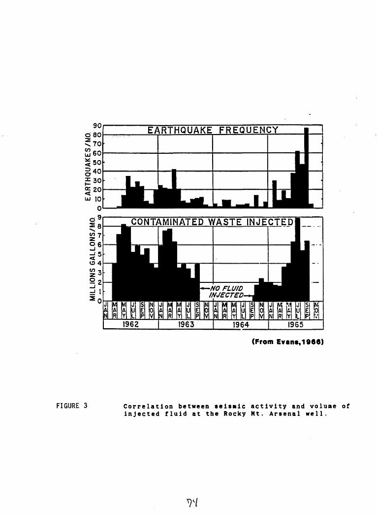
EARTHQUAKE FREQUENCY

CONTAMINATED WASTE INJECTED

NO FLUID INJECTED

(From Evant,1966)

FIGURE 3 Correlation between seisaic activity and volume of injected fluid at the Rocky Nt. Arsenal well.

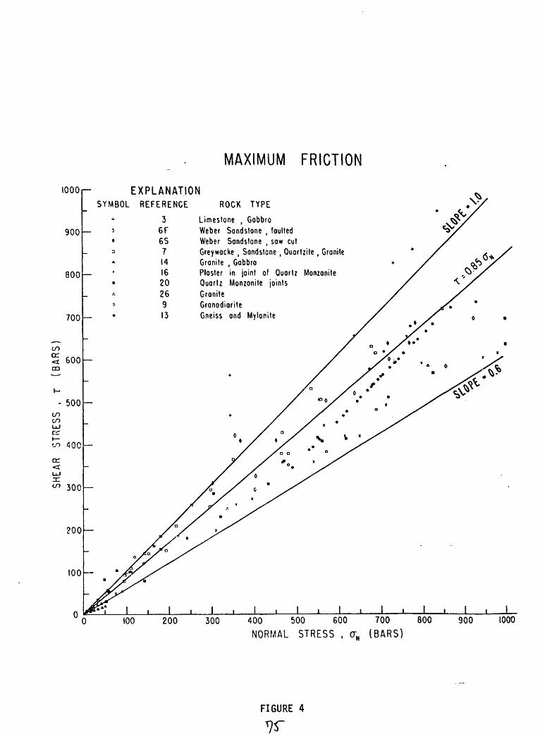
MAXIMUM FRICTION

1000

900 h-

EXPLANATIONSYMBOL REFERENCE ROCK TYPE

Limestone , GobbroWeber Sondstone , foultedWeber Sandstone , sow cutGreywocke , Sondstone , Ouortzite, GraniteGranite , GabbroPlaster in joint of Quartz MonzoniteQuartz Monzonite jointsGraniteGranodioriteGneiss and Mylonite

400 500 600 700 800

NORMAL STRESS , (7N (BARS)

900 1000

FIGURE 4

en c/)UJo: to(T. < UJI CO

NORMAL STRESS (°h)

Op

FIGURE 5 (a) Coulomb's law for failure in dry rock, showing the relationship between the shear stress (x) required for failure and the normal stress an across the plane. Here TO is the cohesion and /* is the coefficient of friction, (b) The Mohr circle diagram, which provides a graphical method by which the principal (compressive) stresses (<rj) can be resolved into shear (T) and normal (o-J components on a plane at angle a to the a3 direction, (c) The Mohr- Coulomb failure criterion. Given maximum (aj and minimum (<r3) principal stresses, failure will occur on a plane containing the intermediate stress (a2) and at an angle a to <7 3 if the circle containing points a l and <r 3 intersects the failure curve defined in (a).

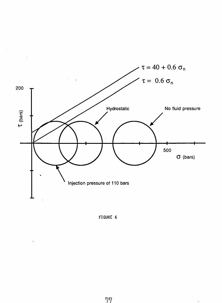
= 40 + 0.6 G n

T= 0.6 G n

200 i-

No fluid pressure

G (bars)

Injection pressure of 110 bars

FIGURE 6

90

PLUM* AND Cox: BOUHOU ELONGATION MBASUUMNTS

82* 78* 74* 70* 66» 62*

Maximum Horizontal Strasa Diractiona

Su Direction Inferred From

Borehole Elongation

Hydraulic Fracture

Overcoring

I Atlantic Coast ' Stress Province

Boundary / (Zoback 4 Zoback. 1960)

90*

B Coring-lnduced Fractures

Borehol* ElongationsN32»W±8-

19 WeNs: 0.1-4.5 Km

Centerline FracturesN58*E± 10*21 Wells; 0.1 -2.0 Km

Hydraulic Fractures

Approximate Edge ol N65*E * 8*Silurian Salt: 30 Wells; 0.025-1.5 Km75 m Isopach

EGSP Well Number

Strike ol Centerline Fractures

Appalachian Fold Belt

GrenviMe & Kenoran Fold Belts

Coastal Plain

FIGURE 7

100 _____ 0 ______ 100 Miles

100 0 100 Kilometers

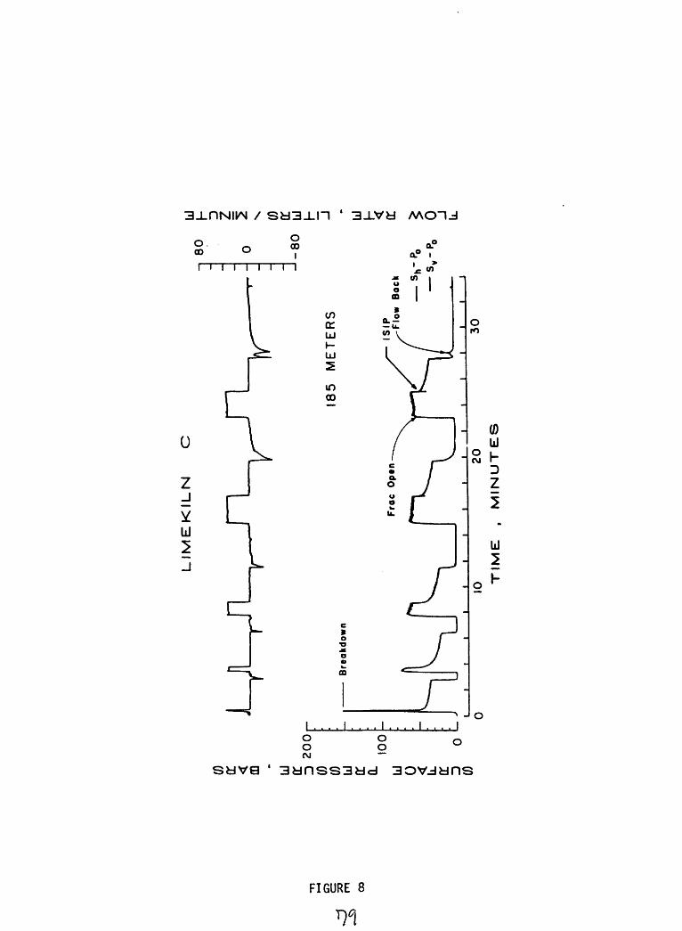
Mi

SURFACE PRESSURE , BARS

o o

ro O O

CD

j

I

m

IzcH 1°

m0)

rI m ^r Z

0

0001

mHm

i i i i i i i

io00o

FLOW RATE , LITERS / MINUTE

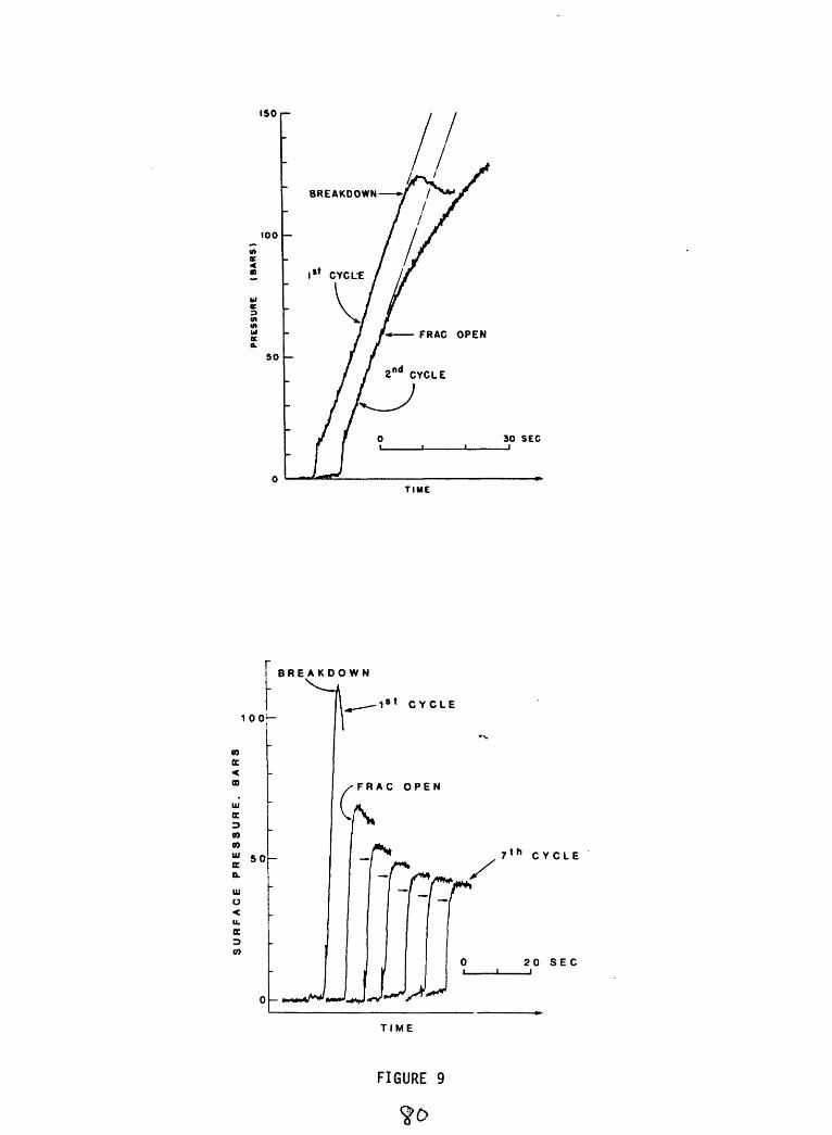
150 r-

100

50

BREAKDOWN

I st CYCLE

30 SEC

TIME

BREAK DOWN

1 st CYCLE

7 th CYCLE

20 SEC

TIME

FIGURE 9

200

100

TYPE 1: FRAG OPEN 2 Sh e.g. Mojave 1: 185 m

Breakdown

Frac Opan v

50

0

-50

10 20 30

a. fJL_n100

50

_ TYPE 2: FRAC OPEN < SH e.g. Crystallaire: 338 m

QLJ

Breakdown

Frac Open,.

10 20

50

0

-50

30

-50 150r TYPE 3: FRAC OPEN < S H . BREAKDOWN <Sh e.g. Crystallaire: 751 m

Breakdown

100

10 20 TIME . MINUTES

30

FIGURE 10

MA

XIM

UM

H

OR

IZO

NT

AL

C

OM

PR

ES

SIV

E

ST

RE

SS

FOC

AL

ME

CH

AN

ISM

IN

S

ITU

S

TR

ES

S

GE

OL

OG

IC

MIX

ED

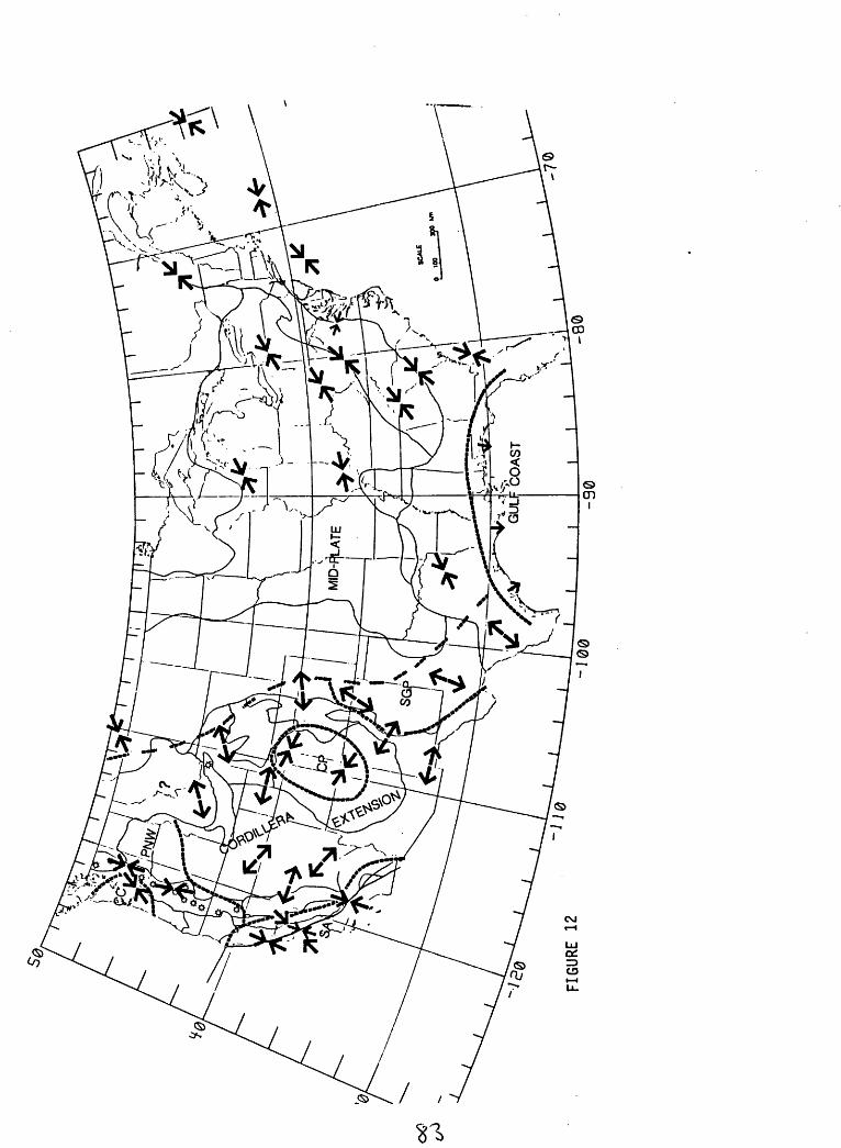
-100

-90

-80

INJECTION

PRESSURE

Radius,

cms

12.1

8 9

10

11

12

13

14

IS

16

17

18

19

20

21

22

23

24

25

Tim

e,

years

FIGU

RE

13

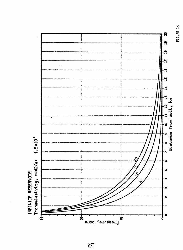
INFINITE R

ESERVOIR

Transmlsslvlty,

m*M2

/8:

4.5x

10"

67

8 9

10

11

12

13Di

stan

ce fr

om we

ll,

km15

16

17

18

19

20

FIGURE 14

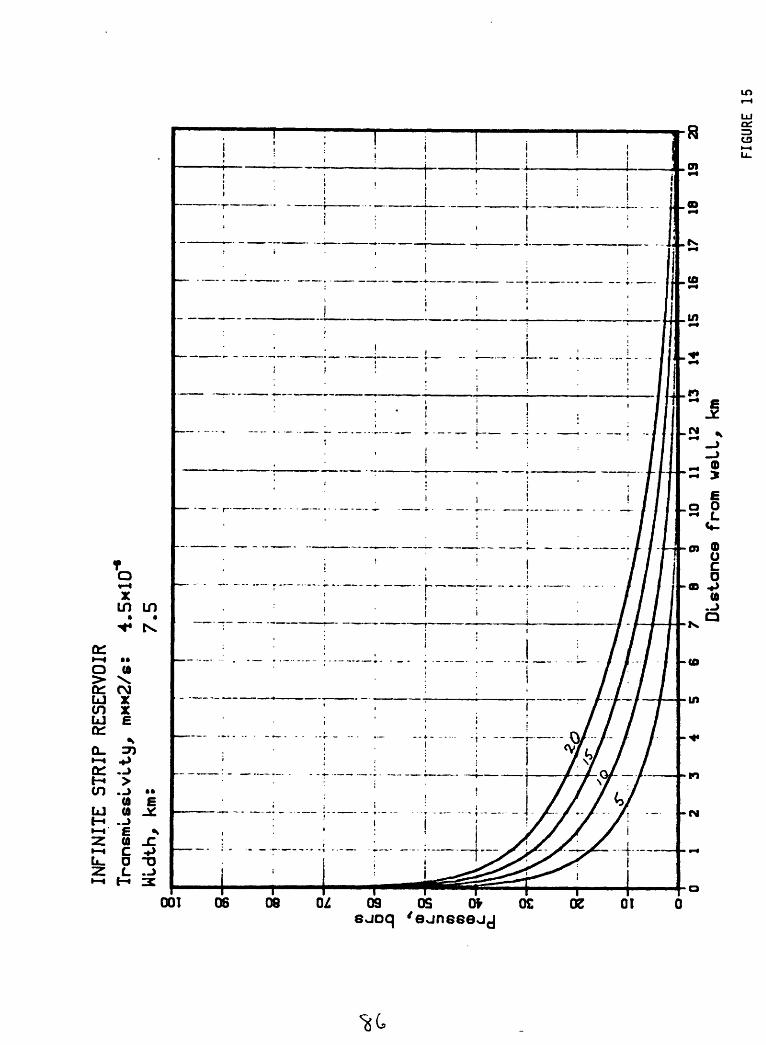
oO

INFINITE S

TRIP R

ESERVOIR

Tran

smls

slvl

ty,

mn*2/s:

4.5x10"*

Widt

h, km

: 7.

5

7 8

9 10

11

12

13

Distance from well, km

li

15

16

17

18

19

20

FIGU

RE 15

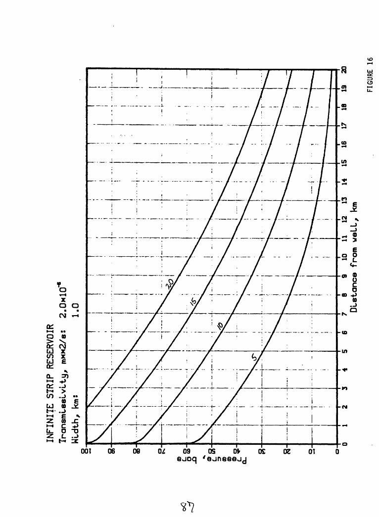
INFINITE S

TRIP R

ESER

VOIR

Tr

ansm

lssl

vlti

j, m**2/8:

2.0*

10

Width, km

: 1.0

6 7

8 9

10

11

12

13

14

15

16

Distance from well, km

18

19

20

FIG

UR

E 16

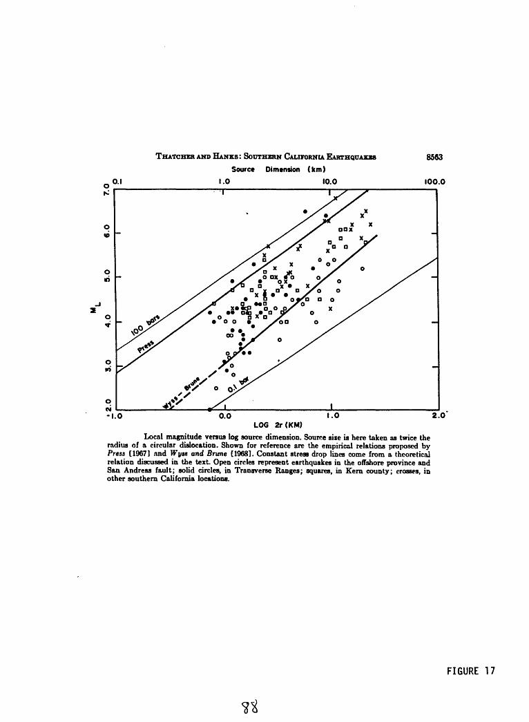
O.I

THATCHER AND HANKS: SOUTHERN CALIFORNIA EARTHQUAKESSource Dimension (km)

1.0 10.0

8563

100.0

2.0LOG 2r(KM)

Local magnitude versus log source dimension. Source size is here taken as twice the radius of a circular dislocation. Shown for reference are the empirical relations proposed by Press [1967] and Wyss and Brvne [1968]. Constant stress drop lines come from a theoretical relation discussed in the text. Open circles represent earthquakes in the offshore province and San Andreas fault; solid circles, in Transverse Ranges; squares, in Kern county; crosses, in other southern California locations.

FIGURE 17

STfl

TION

=002

0.0

20 r

0.0

15

-

to c.

-s

n> oo

o0.0

10

-

o.oo

s -

0 L

H=

0

H=

90

26

28

30

TIM

E

(UT

)=1

98

6:0

71

:08

:55

+

SE

CO

ND

S

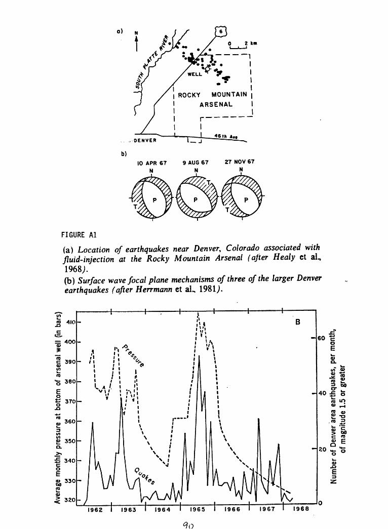
Aver

age

mon

thly

pre

ssur

e at

bot

tom

of

arse

nal w

ell

(in b

ars)

W

CMf\J

O

lO

O

Ol

01

oi

.U

Ul

O>o

o

oO

l

0

tt

E> 1' 1

Si

^

«.5*

3

?

o 53

(^

£.0 g

"*^

"^

U> O

0) O <

0)

n

7) 0 o X -^ ' MOUNl

ARSENAL

>

z

X

'<

\MP

i X

Vr ^

.,5

1

<*o

Num

ber

of D

enve

r ar

ea e

arth

quak

es,

per

mon

th,

of m

agni

tude

1.5

or

grea

ter

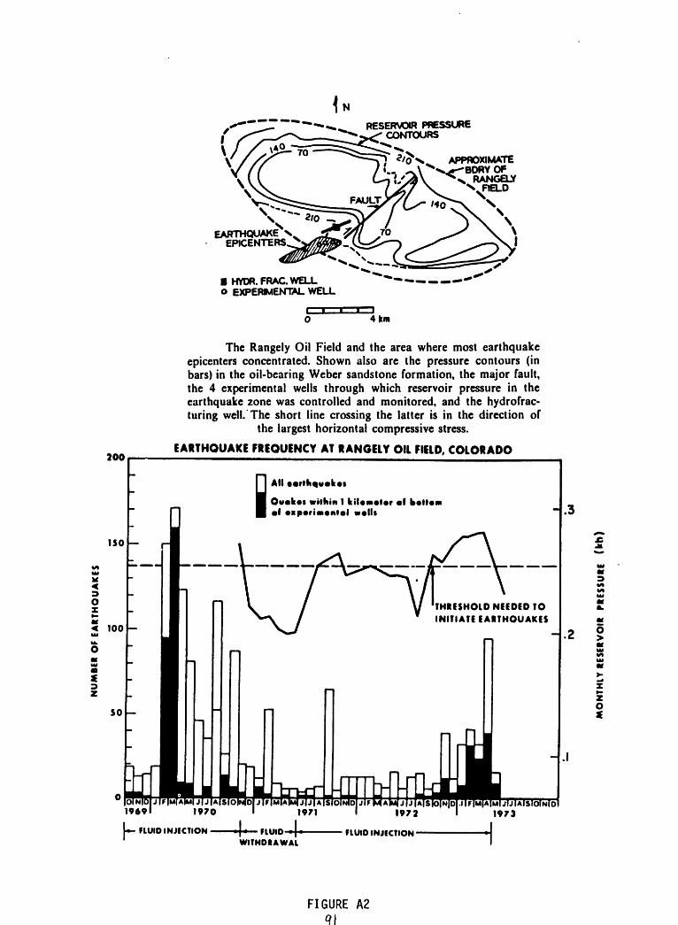
RESERVOIR PRESSURE CONTOURS

v * -,.:;N 2/0

EARTHQUAKE^ EPICENTERS x

APPROXIMATEOF

RANG6LY N FIELD

N

\

+'

HYOR.FRAC.WELL o EXPERIMENTAL WELL

4km

200

The Rangely Oil Field and the area where most earthquake epicenters concentrated. Shown also are the pressure contours (in bars) in the oil-bearing Weber sandstone formation, the major fault, the 4 experimental wells through which reservoir pressure in the earthquake zone was controlled and monitored, and the hydrofrac- turing well. The short line crossing the latter is in the direction of

the largest horizontal compressive stress.

EARTHQUAKE FREQUENCY AT RANGELY OIL FIELD, COLORADO

ISO

< 100

SO

iAll orlfiqwok««

Owok«t within 1 kilometer of botUm of pcrimonlol ««lli

TMIESMOID NEEDED TO INITIATE IAlfMOUAKES

.3

.2

1969

FLUID INJECTION FLUID-

1972

FLUID INJICTION-

1973

WITHDRAWAL

FIGURE A2

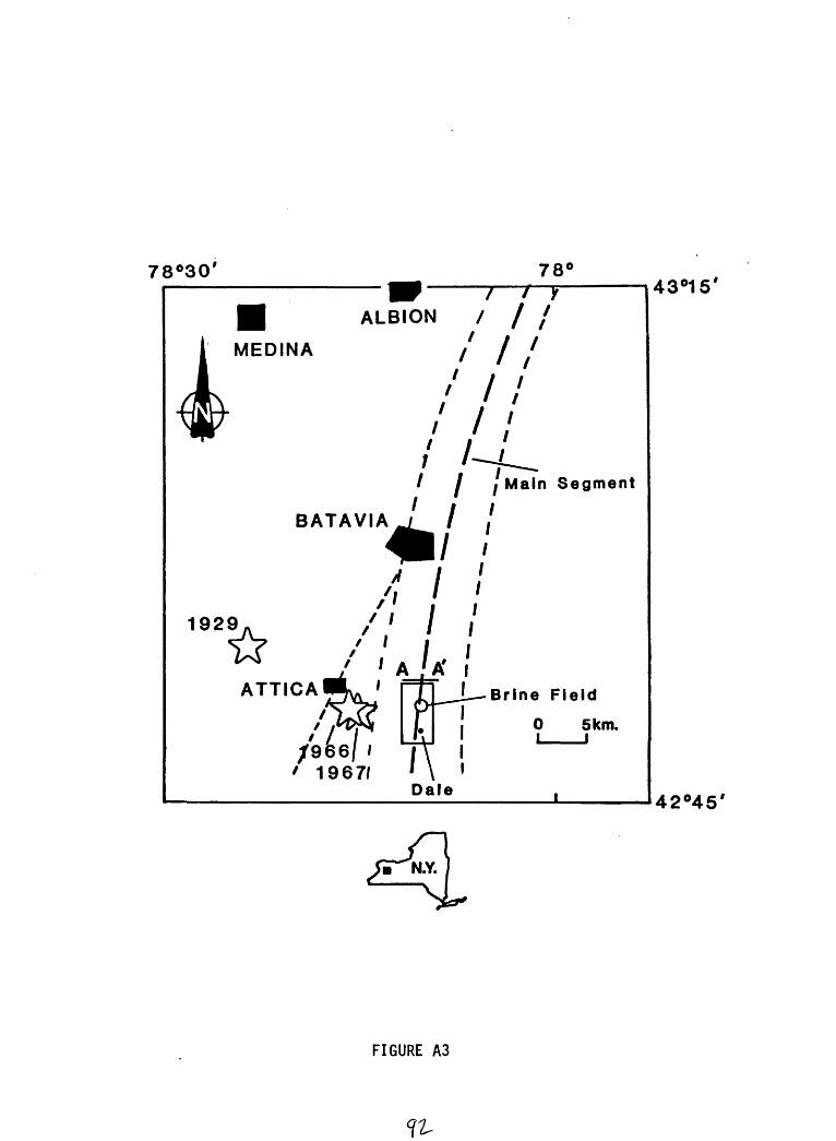
78°30' 78'

7 7F43°15'

ALBION

MEDINA

Main Segment

BATAVIA

ATTICA

5km.

966 ' 1967/

Dale 42°45'

N.Y.

FIGURE A3

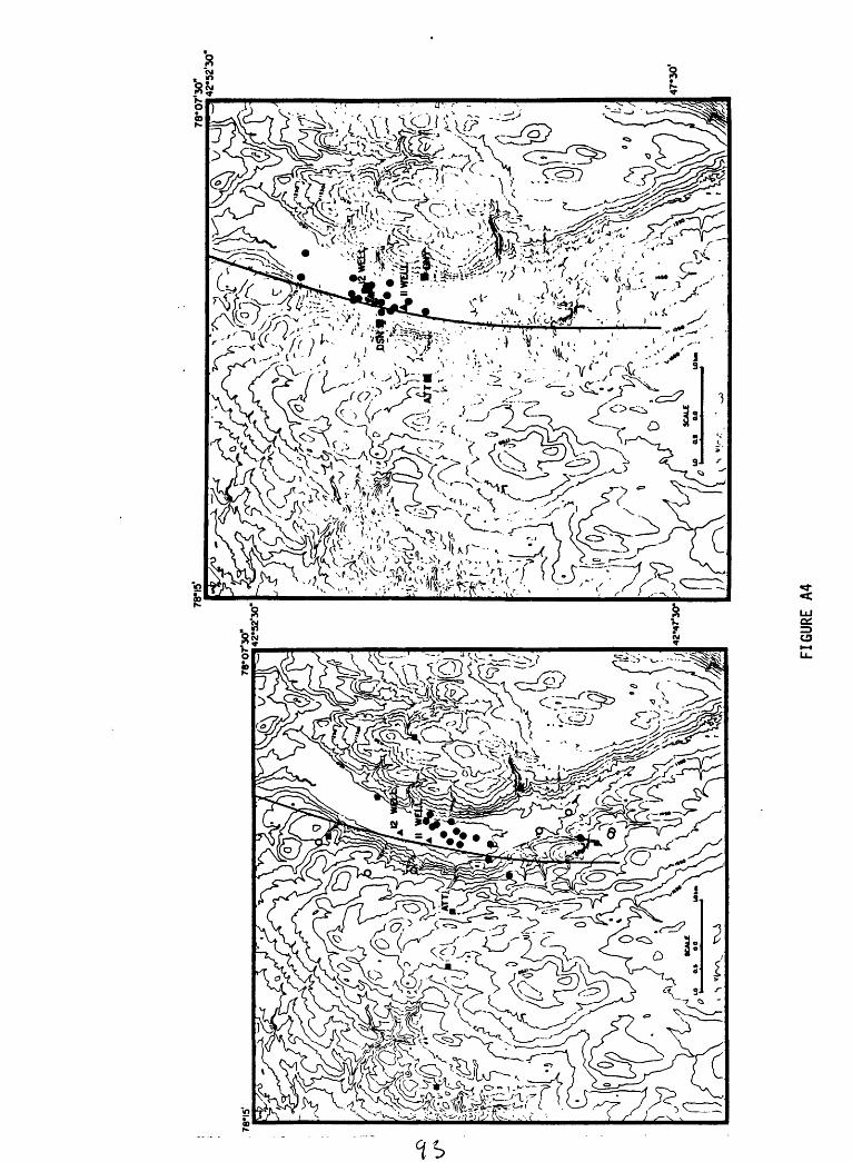
78-1

5'

78*1

5'

*S*

^

78*0

7'3O

"42

*52*

30"

42*4

7*30

*

3?^f

^K^r

ifi]

' d&\

$ k^ Aj

y/^v

-1 \

v "\N

C«

i /

>-vy

78*0

7*30

"

^ v

fe' J

^^/f»

^

.fc-

'>- . -

A-*r

r"

' M

Is r

. ^f

y-xY

V/^

v.M

Ww /^

u^

y^^i

$ y&

. v

if '

; >:-

ft v -

" '

^ v-

,\ \ ^

u.to

\ i\ \

I [ >-

x

X f^

-

42*5

230

47*3

0'

FIG

UR

E A

4

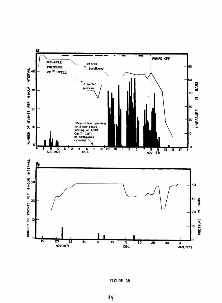
NU

MB

ER

OF

EV

EN

TS

PER

6

HO

UR

IN

TER

VA

L

I8

5

ino N

rv>

o01

o

NU

MB

ER

OF

EV

EN

TS

PER

O

O

6 H

OU

R

INTE

RV

AL

I

PR

ES

SU

RE

ro

CMo

o

IN

BA

RS

PR

ES

SU

RE

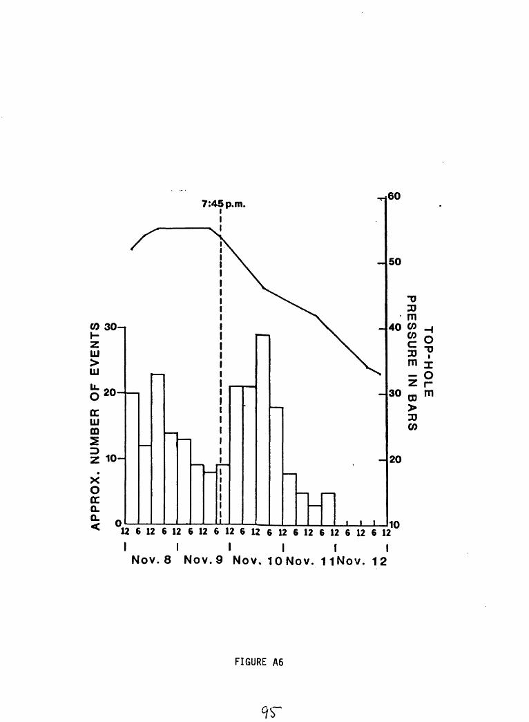
TOP-HOLE

PRESSURE IN

BARS

CMozozOOZo>oZ

00oz

vo<cLU

S1N

3A

3

dO

^

c>

104*

31°

Ear

thqu

akes

loc

ated

aft

er J

anua

ry 1

976

usin

g th

e cu

rren

t op

erat

ing

netw

ork.

Lar

ge X

's a

re

eart

hqua

kes

in t

he r

ange

: 3.

0 <

MLU

£ 4

.0; s

mal

l x'

s: 2

.0 <

MLD

£ 3

.0; l

arge

+'s:

1.0

< M

Lu £

2.0

; sm

all

-t-'s:

MI.I

> £

1.0

. T

he s

quar

e fi

gure

s in

4 s

izes

ind

icat

e ea

rthq

uake

s in

the

sam

e m

agni

tude

ran

ges

give

n ab

ove

with

the

lar

gest

squ

are

indi

catin

g th

e la

rges

t ra

nge.

Ear

thqu

akes

ind

icat

ed b

y a

squa

re a

re l

ess

relia

ble

with

a q

ualit

y of

C o

r D

and

gap

>18

0°. A

ll oi

l fie

lds

are

indi

cate

d by

sol

id li

nes,

and

the

loca

tion

of s

ever

al m

ajor

fie

lds

is s

how

n.

31C

103°

O

DIS

POSA

L SI

TE PECO

S

0 10

20

30

40

50

i ' ' >

' i

Kilo

met

ers

31*

104*

1034

All

loca

ted

eart

hqua

kes

and

infe

rred

pre

-Per

mia

n fa

ults

tak

en f

rom

a 1

:960

0 sc

ale

map

pr

ovid

ed b

y G

eom

ap C

orp.

(R

. D

. W

ilde,

wri

tten

com

mun

icat

ion)

. T

he r

ecta

ngul

ar f

igur

e en

clos

es t

he

even

ts t

hat

are

show

n in

cro

ss s

ectio

n in

Fig

ure

7. L

arge

X's

are

eart

hqua

kes

in t

he r

ange

: 3.

0 <

MLU

2

4.0;

sm

all

x's:

2.0

< M

LD £

3.0

; lar

ge -

t-'s:

1.0

< M

m 5

2.0

; sm

all

-t-'s:

Mm

£ 1

.0. T

he s

quar

e fi

gure

s in

4

size

s in

dica

te e

arth

quak

es i

n th

e sa

me

mag

nitu

de r

ange

s gi

ven

abov

e w

ith t

he l

arge

st s

quar

e in

dica

ting

the

larg

est

rang

e. E

arth

quak

es i

ndic

ated

by

a sq

uare

are

les

s re

liabl

e w

ith a

qua

lity

of C

or

D a

nd g

ap

FIG

UR

E A7

^STATIOKS

EARTHQUAKES

Oil PRODUCING

WATER FlOODWG

10WO

Earthquake epicenters in the Cogdell oil field Handing (1981). From

FIGURE A8

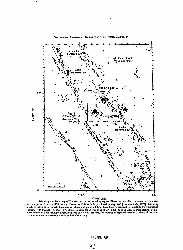
OPPENHHMER: EXTENSIONAL TECTONICS AT THE GEYSERS, CALIFORNIA

ACOLLAYOMIFLT.

S-^MERCURYVILLE»

123 122°

LONGITUDESeismicity and fault map of The Geysers and surrounding region. Pluses outside of box represent earthquakes

for time period January 1976 through December 1984 with M 2: 1.5 and quality A-C [Lee and Lahr, 1975]. Seismicity inside box depicts earthquake locations for which fault plane solutions have been determined in this study for time period January 1984 through October 1985. Open triangles depict locations of CALNET stations used in computation of fault plane solutions. Solid triangles depict locations of stations used only for location of regional Seismicity. Many of the latter stations were not in operation during period of this study.

FIGURE A9

OPP

ENHE

IMER

: EX

TENS

IONA

L TE

CTON

ICS

AT T

HE G

EYSE

RS, C

ALIF

ORN

IA

J I I_____I_

____I_

____1_____I_

____L

OPP

CN

HB

MER

: E

TRM

ION

AL

TIC

TOM

CS

AT T

HE

GEYS

ERS.

CAL

IFO

RN

IA

I__

__

_I_

__

__

I

19

76

1977

19

78

1979

19

80

19

81

1

98

2

1983

19

84

TIM

EY

earl

y ne

t m

ass

of w

ater

w

ithdr

awn

com

pare

d w

ith

the

year

ly

num

ber

of e

arth

quak

es

Ma

1.2

and

qual

ity »

A-C

[L

ie a

nd L

ahr.

I97S

] an

d th

e as

soci

ated

mom

ent

sum

(Ta

ble

2) f

or e

ntir

e Th

e G

eyse

rs g

eolh

erm

al

rese

rvoi

r. T

he p

rese

nce

of a

few

M3

+ ea

rthq

uake

s gr

eatly

influ

ence

s th

e m

omen

t sum

cal

cula

tion

and

expl

ains

the

bet

ter

corr

elat

ion

betw

een

year

ly m

ass

with

draw

n an

d nu

mbe

r of

eart

hqua

kes.

1976

1977

1978

1979

1980

1981

1982

1983

1984

TIME

Mon

thly

num

ber

of k

Wh

elec

tric

ity g

ener

ated

at

P.G

. A

E u

nit

15 (

Paci

fic G

as a

nd E

lect

ric,

per

sona

l co

mm

unic

atio

n. 1

985)

com

pare

d w

ith t

he n

umbe

r of

ear

thqu

akes

M 2

1.2

and

qual

ity -

A-C

[L

et a

nd L

ahr,

1975

] pe

r m

onth

and

the

ass

ocia

ted

mom

ent

sum

. N

ote

incr

ease

of

seism

icity

fol

low

ing

com

men

cem

ent

of p

ower

gen

erat

ion

aad

subs

eque

nt a

bate

men

t of s

eism

icity

follo

win

g th

e dec

reas

e in

the n

umbe

r of

kW

h ge

nera

ted.

FIGU

RE A

10

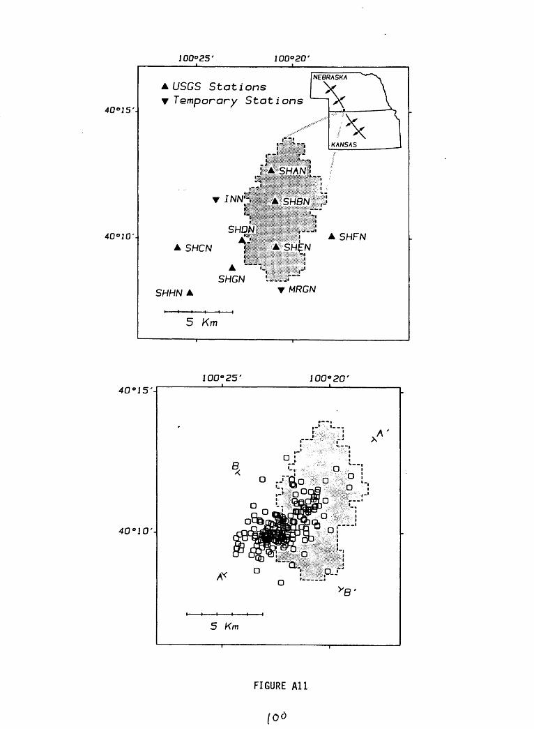
o

§o §

E:*:LO

o

f\jo -

OOin f\j0

-

O

O

LiJa

: O

O

.. Ein

in «oO

in0O0O

o O

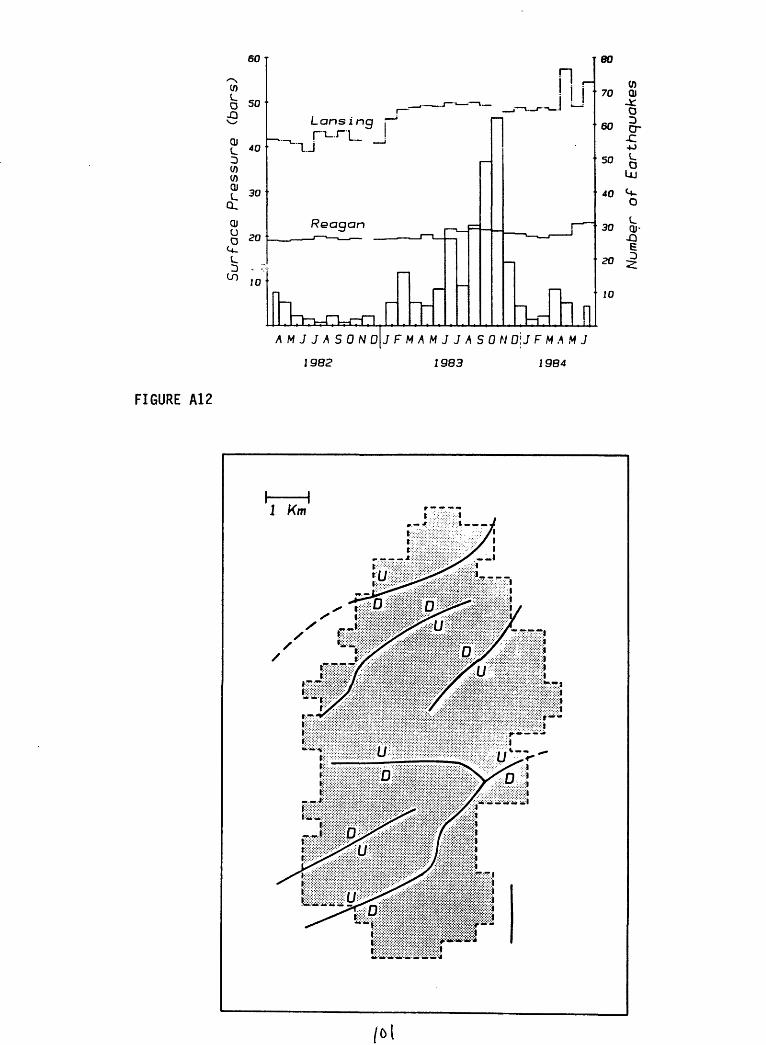
50 m 3> H-»

no

Surf

ocQ

Pres

sure

(b

ars)

CO

O

CO

CD

CO>. CO

O

(O

CD

r-J 7

g h «

r~ >-

i.i

3 .

CO O>

si

O

O

Numb

er of

Earthquakes

Location map of Gobies oil field in Southwestern Ontario. The oil trap occurs as a pinch-out of an Upper Cambrian Sandstone formation on the Appalachian side of the Algonquin arch. Seismic stations of the University of Western Ontario permanent seismic array are DLA, LDN, and ELF.

STATION 1 STATION 2 LOCATION OF EPICENTERS

Gobies earthquake epicenter map.

FIGURE A13

(VL

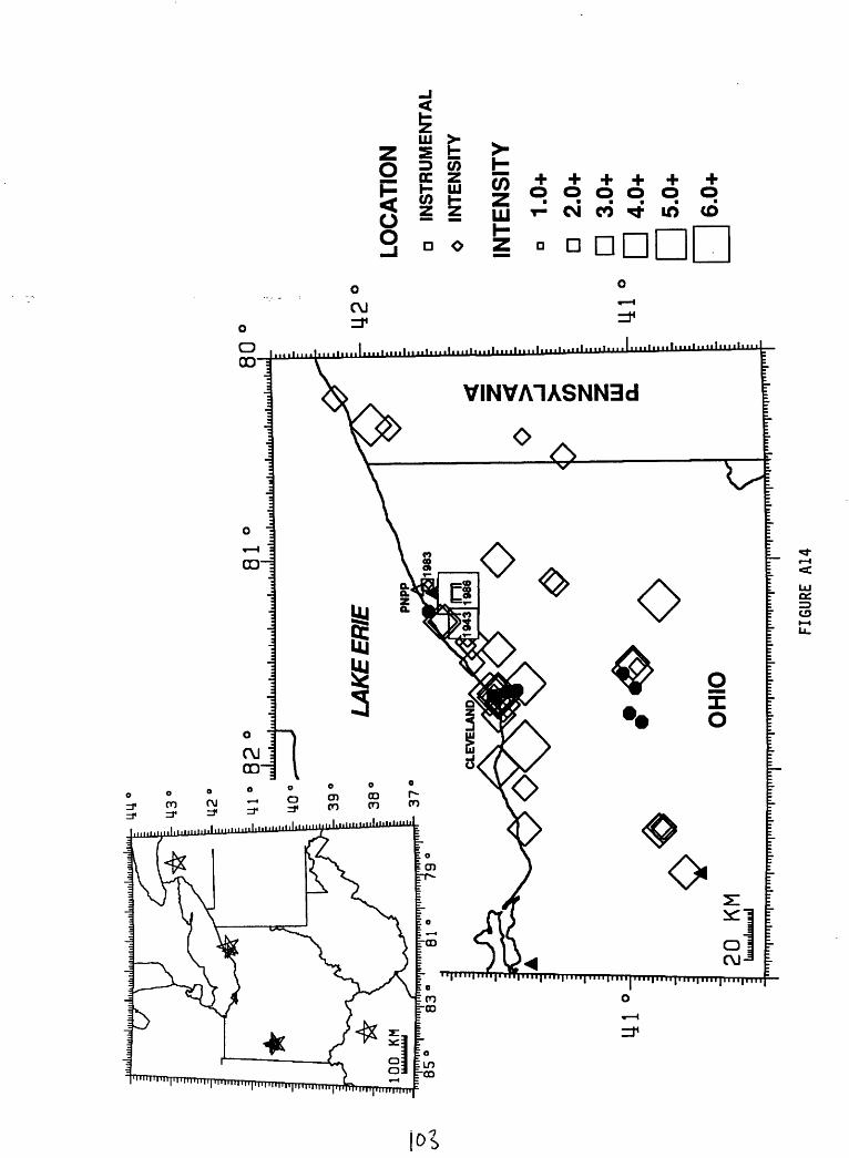
I*)

CD<= »m

PENNSYLVANIA

D nO n

o> 01 ^ GO 10 -» EJ ^^o o o o o o ^

og m H

Z 30(/> C

I

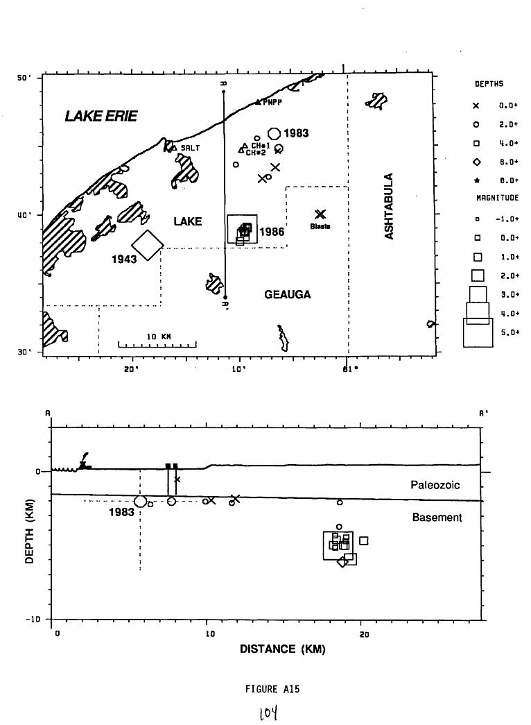
SO 1 -

30' H

DEPTHS

X 0.0+

O 2.0+

4.0+

8.0+

* 8.0+

MRGNITUDE

D

O

D

a0.0+

2.0+

3.D+

4.0+

5.0+

r 20 10

0

Paleozoic

Q.HIQ

-10

1983o

D

Basement

10

DISTANCE (KM)20

FIGURE A15

«/» l5zUJ

UJ

ti_ i n0 l °

DCUJa23Z 5«j

0

i i i i i i

fc

1971

, , , 1 1

i i i i i

-

JAN F£3 -V.AR APRIL WAY JU.Nc JULY AUG SEPT OCT NOV DEC

1 s

O cS J

IS7I

(From T«ng «t a I., 1973)

FIGURE A16 Correlation of seismic activity with net fluid Injection at the Inglewood Oil Field. CA.

(Ob"

38"

70"

20

55/0

8/2

1

5.0

56

/09

/22

5.

39

/09

/20

H

62

/06

/19

4.

4

72/1

1/27

4.

466

/08/

11

4.2

_63

/06/

11

44

66/0

8/10

4.

9 .

72/0

5/3

0

4.7 69

/01/

21

4.9

-75/

03/1

44.

1 -7

2/11

/06

4.3

75/1

0/25

4.

4

77/0

3/0

8

4.7

77

/03

/09

" 4

.07

3/0

4/0

2

1*4.

0

38

'45

'N

38'0

0'

69

'00

'E6

9'4

5'

FIG

UR

E B

l

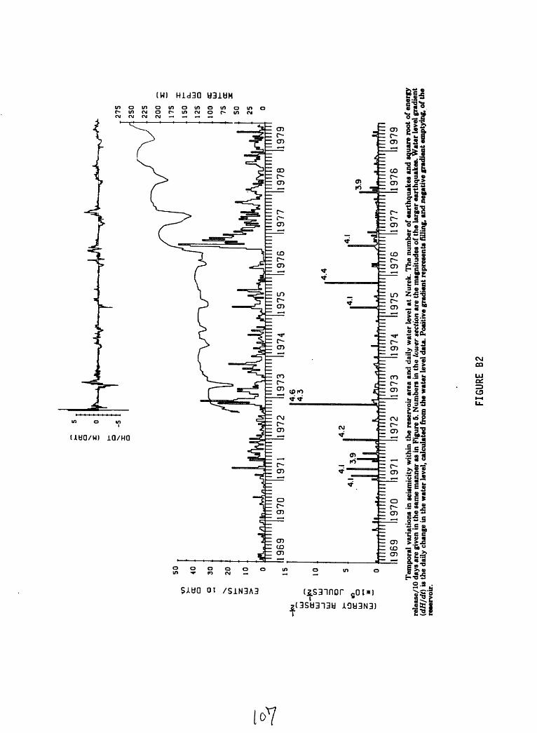
50

1974

19

75

1976

19

77

X

t

0.

LU a

cc

111

1979

Tem

pora

l va

riat

ions

in s

eism

icity

with

in t

he r

eser

voir

are

a an

d da

ily w

ater

leve

l at

Nur

ek. T

he n

umbe

r of

ear

thqu

akes

and

squ

are

root

of e

nerg

y re

leas

e/10

day

s ar

e gi

ven

in t

he s

ame

man

ner

as in

Fig

ure

5. N

umbe

rs in

the

low

er s

ectio

n ar

e th

e m

agni

tude

s of

the

larg

er e

arth

quak

es. W

ater

leve

l gra

dien

t (d

H/d

t) i

s th

e da

ily c

hang

e in

the

wat

er le

vel,

calc

ulat

ed fr

om t

he w

ater

leve

l dat

a. P

osit

ive

grad

ient

rep

rese

nts

fillin

g, a

nd n

egat

ive

grad

ient

em

ptyi

ng, o

f the

re

serv

oir.

FIG

UR

E B2