Embed Size (px)
Citation preview
Ž .JOURNAL OF ALGORITHMS 25, 19]51 1997ARTICLE NO. AL970873
A Reliable Randomized Algorithm for theClosest-Pair Problem
Martin Dietzfelbinger*
Fachbereich Informatik, Uni ersitat Dortmund, D-44221 Dortmund, Germany¨
Torben Hagerup†
Max-Planck-Institut fur Informatik, Im Stadtwald, D-66123 Saarbrucken, Germany¨ ¨
Jyrki Katajainen‡
Datalogisk Institut, Københa ns Uni ersitet, Uni ersitetsparken 1,DK-2100 Københa n Ø, Denmark
and
Martti Penttonen§
Tietojenkasittelytieteen laitos, Joensuun yliopisto, PL 111, FIN-80101 Joensuu, Finland¨
Received December 8, 1993; revised April 22, 1997
The following two computational problems are studied:Duplicate grouping: Assume that n items are given, each of which is labeled by an
� 4integer key from the set 0, . . . , U y 1 . Store the items in an array of size n suchthat items with the same key occupy a contiguous segment of the array.
Closest pair: Assume that a multiset of n points in the d-dimensional Euclideanspace is given, where d G 1 is a fixed integer. Each point is represented as a
� 4 Ž .d-tuple of integers in the range 0, . . . , U y 1 or of arbitrary real numbers . Find aclosest pair, i.e., a pair of points whose distance is minimal over all such pairs.
* Partially supported by DFG grant Me 872r1-4.† Partially supported by the ESPRIT Basic Research Actions Program of the EC under
Ž .contract 7141 project ALCOM II .‡ ŽPartially supported by the Academy of Finland under contract 1021129 project Efficient
.Data Structures and Algorithms .§ Partially supported by the Academy of Finland.
19
0196-6774r97 $25.00Copyright Q 1997 by Academic Press
All rights of reproduction in any form reserved.
DIETZFELBINGER ET AL.20
In 1976, Rabin described a randomized algorithm for the closest-pair problemthat takes linear expected time. As a subroutine, he used a hashing procedurewhose implementation was left open. Only years later randomized hashing schemessuitable for filling this gap were developed.
In this paper, we return to Rabin’s classic algorithm to provide a fully detaileddescription and analysis, thereby also extending and strengthening his result. As apreliminary step, we study randomized algorithms for the duplicate-groupingproblem. In the course of solving the duplicate-grouping problem, we describe anew universal class of hash functions of independent interest.
It is shown that both of the foregoing problems can be solved by randomizedŽ . Ž .algorithms that use O n space and finish in O n time with probability tending to
1 as n grows to infinity. The model of computation is a unit-cost RAM capable ofgenerating random numbers and of performing arithmetic operations from the set� 4q, y, ), DIV, LOG , EXP , where DIV denotes integer division and LOG and EXP2 2 2 2
� 4 Ž . ? @ Ž . mare the mappings from N to N j 0 with LOG m s log m and EXP m s 22 2 2for all m g N. If the operations LOG and EXP are not available, the running time2 2
Ž .of the algorithms increases by an additive term of O log log U . All numbersŽ .manipulated by the algorithms consist of O log n q log U bits.
Ž .The algorithms for both of the problems exceed the time bound O n orŽ . yn VŽ1.
O n q log log U with probability 2 . Variants of the algorithms are also givenŽ . Ž ya .that use only O log n q log U random bits and have probability O n of
exceeding the time bounds, where a G 1 is a constant that can be chosenarbitrarily.
The algorithms for the closest-pair problem also works if the coordinates of thepoints are arbitrary real numbers, provided that the RAM is able to perform
� 4arithmetic operations from q, y, ), DIV on real numbers, where a DIV b now? @ Ž .means arb . In this case, the running time is O n with LOG and EXP and2 2
Ž Ž ..O n q log log d rd without them, where d is the maximum and d ismax max max minthe minimum distance between any two distinct input points. Q 1997 Academic Press
1. INTRODUCTION
The closest-pair problem is often introduced as the first nontrivial prox-w ximity problem in computational geometry}see, e.g., 26 . In this problem
we are given a collection of n points in d-dimensional space, where d G 1is a fixed integer, and a metric specifying the distance between points. Thetask is to find a pair of points whose distance is minimal. We assume thateach point is represented as a d-tuple of real numbers or of integers in afixed range, and that the distance measure is the standard Euclideanmetric.
w xIn his seminal paper on randomized algorithms, Rabin 27 proposed analgorithm for solving the closest-pair problem. The key idea of the algo-rithm is to determine the minimal distance d within a random sample of0points. When the points are grouped according to a grid with resolutiond , the points of a closest pair fall in the same cell or in neighboring cells.0This considerably decreases the number of possible closest-pair candidates
A RANDOMIZED ALGORITHM FOR CLOSEST PAIRS 21
Ž .from the total of n n y 1 r2. Rabin proved that with a suitable samplesize the total number of distance calculations performed will be of order nwith overwhelming probability.
A question that was not solved satisfactorily by Rabin is how the pointsare grouped according to a d grid. Rabin suggested that this could be0implemented by dividing the coordinates of the points by d , truncating the0quotients to integers, and hashing the resulting integer d-tuples. Fortune
w xand Hopcroft 15 , in their more detailed examination of Rabin’s algo-Ž .rithm, assumed the existence of a special operation FINDBUCKET d , p ,0
which returns an index of the cell into which the point p falls in some� 4fixed d grid. The indices are integers in the range 1, . . . , n , and distinct0
cells have distinct indices.Ž w x.On a real RAM for the definition, see 26 , where the generation of
'� 4random numbers, comparisons, arithmetic operations from q, y, ), r, ,and FINDBUCKET require unit time, Rabin’s random-sampling algorithm
Ž . w x Žruns in O n expected time 27 . Under the same assumptions theŽ .closest-pair problem can even be solved in O n log log n time in the worst
w x .case, as demonstrated by Fortune and Hopcroft 15 . We next introduceterminology that allows us to characterize the performance of Rabin’salgorithm more closely. Every execution of a randomized algorithm suc-ceeds or fails. The meaning of ‘‘failure’’ depends on the context, but anexecution typically fails if it produces an incorrect result or does not finishin time. We say that a randomized algorithm is exponentially reliable if, oninputs of size n, its failure probability is bounded by 2yn «
for some fixed« ) 0. Rabin’s algorithm is exponentially reliable. Correspondingly, analgorithm is polynomically reliable if, for every fixed a ) 0, its failureprobability on inputs of size n is at most nya . In the latter case, we allowthe notion of success to depend on a ; an example is the expression ‘‘runs
Žin linear time,’’ where the constant implicit in the term ‘‘linear’’ may and.usually will be a function of a .
Recently, two other simple closest-pair algorithms were proposed byw x w xGolin et al. 16 and Khuller and Matias 19 ; both algorithms offer linear
expected running time. Faced with the need for an implementation of theFINDBUCKET operation, these papers employed randomized hashing
w xschemes that had been developed in the meantime 8, 14 . Golin et al.presented a variant of their algorithm that is polynomially reliable, but has
Ž . Žrunning time O n log nrlog log n this variant utilizes the polynomiallyw x.reliable hashing scheme of 13 .
The preceding time bounds should be contrasted with the fact that inŽthe algebraic computation-tree model where the available operations are
'� 4comparisons and arithmetic operations from q, y, ), r, , but where. Ž .indirect addressing is not modeled , Q n log n is known to be the com-
DIETZFELBINGER ET AL.22
plexity of the closest-pair problem. Algorithms proving the upper boundw xwere provided, for example, by Bentley and Shamos 7 and Schwarz et al.
w x30 . The lower bound follows from the corresponding lower bound derivedw x Ž .for the element-distinctness problem by Ben-Or 6 . The V n log n lower
w xbound is valid even if the coordinates of the points are integers 32 or ifw xthe sequence of points forms a simple polygon 1 .
The present paper centers on two issues: First, we completely describean implementation of Rabin’s algorithm, including all the details of thehashing subroutines, and show that it guarantees linear running timetogether with exponential reliability. Second, we modify Rabin’s algorithmso that only very few random bits are needed, but still a polynomialreliability is maintained.1
As a preliminary step, we address the question of how the grouping ofŽ .points can be implemented when only O n space is available and the
strong FINDBUCKET operation does not belong to the repertoire of availableoperations. An important building block in the algorithm is an efficient
Žsolution to the duplicate-grouping problem sometimes called the semisort-.ing problem , which can be formulated as follows: Given a set of n items,
� 4each of which is labeled by an integer key from 0, . . . , U y 1 , store theitems in an array A of size n so that entries with the same key occupy a
w x w xcontiguous segment of the array, i.e., if 1 F i - j F n and A i and A jw xhave the same key, then A k has the same key for all k with i F k F j.
Note that full sorting is not necessary, because no order is prescribed foritems with different keys. In a slight generalization, we consider theduplicate-grouping problem also for keys that are d-tuples of elements
� 4from the set 0, . . . , U y 1 , for some integer d G 1.We provide two randomized algorithms for dealing with the duplicate-
grouping problem. The first one is very simple; it combines universalw x Ž . w xhashing 8 with a variant of radix sort 2, p. 77ff and runs in linear time
with polynomial reliability. The second method employs the exponentiallyw xreliable hashing scheme of 4 ; it results in a duplicate-grouping algorithm
that runs in linear time with exponential reliability. Assuming that U is apower of 2 given as part of the input, these algorithms use only arithmetic
� 4operations from q, y, ), DIV . If U is not known, we have to spendŽ .O log log U preprocessing time on computing a power of 2 greater than
the largest input number; that is, the running time is linear if U s 22 O Žn..
Alternatively, we get linear running time if we accept LOG and EXP2 2among the unit-time operations. It is essential to note that our algorithms
1 In the algorithms of this paper randomization occurs in computational steps like ‘‘pick a� 4 Ž .random number in the range 0, . . . , r y 1 according to the uniform distribution .’’ Infor-
u vmally we say that such a step ‘‘uses log r random bits.’’2
A RANDOMIZED ALGORITHM FOR CLOSEST PAIRS 23
w xfor duplicate grouping are conser ati e in the sense of 20 , i.e., allŽ .numbers manipulated during the computation have O log n q log U bits.
Technically as an ingredient of the duplicate-grouping algorithms, weintroduce a new universal class of hash functions}more precisely, we
w xprove that the class of multiplicative hash functions 21, pp. 509]512 isw xuniversal in the sense of 8 . The functions in this class can be evaluated
very efficiently using only multiplications and shifts of binary representa-tions. These properties of multiplicative hashing are crucial to its use in
w xthe signature-sort algorithm of 3 .On the basis of the duplicate-grouping algorithms we give a rigorous
analysis of several variants of Rabin’s algorithm, including all the detailsconcerning the hashing procedures. For the core of the analysis, we use anapproach completely different from that of Rabin, which enables us toshow that the algorithm can also be run with very few random bits.Further, the analysis of the algorithm is extended to cover the case of
Žrepeated input points. Rabin’s analysis was based on the assumption that.all input points are distinct. The result returned by the algorithm is always
correct; with high probability, the running time is bounded as follows: On� 4a real RAM with arithmetic operations from q, y, ), DIV, LOG , EXP , the2 2
Ž .closest-pair problem is solved in O n time, and with operations from� 4 Ž Ž ..q, y, ), DIV it is solved in O n q log log d rd time, where d ismax min maxthe maximum and d is the minimum distance between distinct inputmin
Ž ? @points here a DIV b means arb , for arbitrary positive real numbers a. � 4and b . For points with integer coordinates in the range 0, . . . , U y 1 the
Ž .latter running time can be estimated by O n q log log U . For integerdata, the algorithms are again conservative.
The rest of the paper is organized as follows. In Section 2, the algo-rithms for the duplicate-grouping problem are presented. The randomizedalgorithms are based on the universal class of multiplicative hash func-tions. The randomized closest-pair algorithm is described in Section 3 andanalyzed in Section 4. The last section contains some concluding remarksand comments on experimental results. Technical proofs regarding theproblem of generating primes and probability estimates are given inAppendices A and B.
2. DUPLICATE GROUPING
In this section we present two simple deterministic algorithms and tworandomized algorithms for solving the duplicate-grouping problem. As atechnical tool, we describe and analyze a new, simple universal class ofhash functions. Moreover, a method for generating numbers that areprime with high probability is provided.
DIETZFELBINGER ET AL.24
An algorithm is said to rearrange a given sequence of items, each with adistinguishing key, stably if items with identical keys appear in the input inthe same order as in the output. To simplify notation in the followingdiscussion, we will ignore all components of the items except the keys; inother words, we will consider the problem of duplicate grouping for inputsthat are multisets of integers or multisets of tuples of integers. It will beobvious that the algorithms presented can be extended to solve the moregeneral duplicate-grouping problem in which additional data are associ-ated with the keys.
2.1. Deterministic duplicate grouping
We start with a trivial observation: Sorting the keys certainly solves theduplicate-grouping problem. In our context, where linear running time is
w xessential, variants of radix sort 2, p. 77ff are particularly relevant.
w x ŽFACT 2.1 2, P. 79 . The sorting problem and hence the duplicate-grouping. � b 4problem for a multiset of n integers from 0, . . . , n y 1 can be sol ed stably
Ž . Ž .in O b n time and O n space for any integer b G 1. In particular, if b is afixed constant, both time and space are linear.
Remark 2.2. Recall that radix sort uses the digits of the n-ary represen-Ž . wtation of the keys being sorted. To justify the space bound O n instead of
Ž .xthe more natural O b n , observe that it is not necessary to generate andstore the full n-ary representation of the integers being sorted, but that itsuffices to generate a digit when it is needed. Whereas the modulooperation can be expressed in terms of DIV, ), and y, generating such adigit needs constant time on a unit-cost RAM with operations from� 4q, y, ), DIV .
If space is not an issue, there is a simple algorithm for duplicategrouping that runs in linear time and does not sort. It works similarly toone phase of radix sort, but avoids scanning the range of all possible keyvalues in a characteristic way.
LEMMA 2.3. The duplicate-grouping problem for a multiset of n integers� 4from 0, . . . , U y 1 can be sol ed stably by a deterministic algorithm in time
Ž . Ž .O n and space O n q U .
Proof. For definiteness, assume that the input is stored in any array Sof size n. Let L be an auxiliary array of size U, which is indexed from 0 to
ŽU y 1 and whose possible entries are headers of lists this array need not.be initialized . The array S is scanned three times from index 1 to index n.
w w xxDuring the first scan, for i s 1, . . . , n, the entry L S i is initialized tow xpoint to an empty list. During the second scan, the element S i is inserted
w w xxat the end of the list with header L S i . During the third scan, the groups
A RANDOMIZED ALGORITHM FOR CLOSEST PAIRS 25
w w xxare outputted as follows: for i s 1, . . . , n, if the list with header L S i isnonempty, it is written to consecutive positions of the output array and
w w xxL S i is made to point to an empty list again. Clearly, this algorithm runsin linear time and groups the integers stably.
In our context, the algorithms for the duplicate-grouping problem con-sidered so far are not sufficient because there is no bound on the sizes ofthe integers that may appear in our geometric application. The radix-sortalgorithm might be slow and the naive duplicate-grouping algorithm mightwaste space. Both time and space efficiency can be achieved by compress-ing the numbers by means of hashing, as will be demonstrated in thefollowing text.
2.2. Multiplicati e uni ersal hashing
To prepare for the randomized duplicate-grouping algorithms, we de-scribe a simple class of hash functions that is universal in the sense of
w x kCarter and Wegman 8 . Assume that U G 2 is a power of 2, say U s 2 .� 4 � k 4For l g 1, . . . , k , consider the class HH s h N 0 - a - 2 and a is oddk , l a
� k 4 � l 4of hash functions from 0, . . . , 2 y 1 to 0, . . . , 2 y 1 , where h isadefined by
h x s ax mod 2 k div 2 ky l for 0 F x - 2 k .Ž . Ž .a
ky1 Ž .The class HH contains 2 distinct hash functions. Because we assumek , lthat on the RAM model a random number can be generated in constanttime, a function from HH can be chosen at random in constant time, andk , lfunctions from HH can be evaluated in constant time on a RAM withk , l
� 4 Ž k larithmetic operations from q, y, ), DIV for this 2 and 2 must be.known, but not k or l .
The most important property of the class HH is expressed in thek , lfollowing lemma.
� kLEMMA 2.4. Let k and l be integers with 1 F l F k. If x, y g 0, . . . , 2 y41 are distinct and h g HH is chosen at random, thena k , l
1Prob h x s h y F .Ž . Ž .Ž .a a ly12
� k 4Proof. Fix distinct integers x, y g 0, . . . , 2 y 1 with x ) y and ab-� k 4breviate x y y by z. Let A s a N 0 - a - 2 and a is odd . By the
Ž . Ž .definition of h , every a g A with h x s h y satisfiesa a a
k k kylax mod 2 y ay mod 2 - 2 .
DIETZFELBINGER ET AL.26
Ž k . Ž k .Since z k 0 mod 2 and a is odd, we have az k 0 mod 2 . Therefore allsuch a satisfy
k � ky l 4 � k kyl k 4az mod 2 g 1, . . . , 2 y 1 j 2 y 2 q 1, . . . , 2 y 1 . 2.1Ž .
Ž . sTo estimate the number of a g A that satisfy 2.1 , we write z s z92 withz9 odd and 0 F s - k. Whereas the odd numbers 1, 3, . . . , 2 k y 1 form agroup with respect to multiplication modulo 2 k, the mapping
a ¬ az9mod 2 k
is a permutation of A. Consequently, the mapping
a2 s ¬ az92 smod 2 kqs s az mod 2 kqs
� s 4is a permutation of the set a2 N a g A . Thus, the number of a g A thatŽ .satisfy 2.1 is the same as the number of a g A that satisfy
s k � ky l 4 � k kyl k 4a2 mod 2 g 1, . . . , 2 y 1 j 2 y 2 q 1, . . . , 2 y 1 . 2.2Ž .
Now, a2 smod 2 k is just the number whose binary representation is givenby the k y s least significant bits of a, followed by s zeroes. This easily
Ž .yields the following result. If s G k y l, no a g A satisfies 2.2 . ForŽ . ky lsmaller s, the number of a g A satisfying 2.2 is at most 2 . Hence the
Ž .probability that a randomly chosen a g A satisfies 2.1 is at mostky l ky1 ly12 r2 s 1r2 .
Remark 2.5. The lemma says that the class HH of multiplicative hashk , lw x Žfunctions is two-universal in the sense of 24, p. 140 this notion slightly
w x. w x Žgeneralizes that of 8 . As discussed in 21, p. 509 ‘‘the multiplicative.hashing scheme’’ , the functions in this class are particularly simple to
evaluate, because the division and the modulo operation correspond toselecting a segment of the binary representation of the product ax, whichcan be done by means of shifts. Other universal classes use functions that
w x w xinvolve division by prime numbers 8, 14 , arithmetic in finite fields 8 ,w xmatrix multiplication 8 , or convolution of binary strings over the two-
w xelement field 22 , i.e., operations that are more expensive than multiplica-tions and shifts unless special hardware is available.
It is worth noting that the class HH of multiplicative hash functions mayk , lbe used to improve the efficiency of the static and dynamic perfect-hashing
w x w xschemes described in 14 and 12 , in place of the functions of the typeŽ .x ¬ ax mod p mod m, for a prime p, which are used in these papers and
which involve integer division. For an experimental evaluation of thisw x w xapproach, see 18 . In another interesting development, Raman 29 showed
that the so-called method of conditional probabilities can be used to
A RANDOMIZED ALGORITHM FOR CLOSEST PAIRS 27
Ž .obtain a function in HH with desirable properties ‘‘few collisions’’ in ak , lŽdeterministic manner previously known deterministic methods for this
w x.purpose use exhaustive search in suitable probability spaces 14 ; thisallowed him to derive an efficient deterministic scheme for the construc-tion of perfect hash functions.
In the following lemma is stated a well-known property of universalclasses.
LEMMA 2.6. Let n, k, and l be positi e integers with l F k and let S be a� k 4set of n integers in the range 0, . . . , 2 y 1 . Choose h g HH at random.k , l
Then
n2
Prob h is 1]1 on S G 1 y .Ž . l2
Proof. By Lemma 2.4,
1 n2nProb h x s h y for some x , y g S F ? F .Ž . Ž .Ž . ly1 lž /2 2 2
2.3. Duplicate grouping ¨ia uni ersal hashing
Having provided the universal class HH , we are now ready to describek , lour first randomized duplicate-grouping algorithm.
THEOREM 2.7. Let U G 2 be known and a power of 2 and let a G 1 bean arbitrary integer. The duplicate-grouping problem for a multiset of n integers
� 4in the range 0, . . . , U y 1 can be sol ed stably by a conser ati e randomizedŽ . Ž .algorithm that needs O n space and O a n time on a unit-cost RAM with
� 4arithmetic operations from q, y, ), DIV ; the probability that the time boundis exceeded is bounded by nya . The algorithm requires fewer than log U2random bits.
� 4Proof. Let S be the multiset of n integers from 0, . . . , U y 1 to beuŽ . vgrouped. Further, let k s log U and l s a q 2 log n and assume with-2 2
out loss of generality that 1 F l F k. As a preparatory step, we compute 2 l.The elements of S are then grouped as follows. First, a hash function hfrom HH is chosen at random. Second, each element of S is mappedk , l
� l 4 Ž Ž ..under h to the range 0, . . . , 2 y 1 . Third, the resulting pairs x, h x ,Ž .where x g S, are sorted by radix sort Fact 2.1 according to their second
components. Fourth, it is checked whether all elements of S that have thesame hash value are in fact equal. If this is the case, the third step hasproduced the correct result; if not, the whole input is sorted, e.g., withmerge sort.
DIETZFELBINGER ET AL.28
l Ž .The computation of 2 is easily carried out in O a log n time. The fourŽ . Ž . Ž . Ž .steps of the algorithm proper require O 1 , O n , O a n , and O n time,
Ž .respectively. Hence, the total running time is O a n . The result of theŽ .third step is correct if h is 1]1 on the distinct elements of S, which
happens with probability
n2 1Prob h is 1]1 on S G 1 y G 1 yŽ . al n2
by Lemma 2.6. In case the final check indicates that the outcome of thethird step is incorrect, the call of merge sort produces a correct output inŽ .O n log n time, which does not impair the linear expected running time.
The space requirements of the algorithm are dominated by those of theŽ .sorting subroutines, which need O n space. Whereas both radix sort and
merge sort rearrange the elements stably, duplicate grouping is performedstably. It is immediate that the algorithm is conservative and that thenumber of random bits needed is k y 1 - log U.2
2.4. Duplicate grouping ¨ia perfect hashing
We now show that there is another, asymptotically even more reliable,duplicate-grouping algorithm that also works in linear time and space. Thealgorithm is based in the randomized perfect-hashing scheme of Bast and
w xHagerup 4 .The perfect-hashing problem is the following: Given a multiset S :
� 40, . . . , U y 1 , for some universe size U, construct a function h: S ª� < <4 Ž0, . . . , c S , for some constant c, so that h is 1]1 on the distinct
. w xelements of S. In 4 a parallel algorithm for the perfect-hashing problemis described. We need the following sequential version.
w xFACT 2.8 4 . Assume that U is a known prime. Then the perfect-hashing� 4problem for a multiset of n integers from 0, . . . , U y 1 can be sol ed by a
Ž . Ž .randomized algorithm that requires O n space and runs in O n time withprobability 1 y 2yn V Ž1.
. The hash function produced by the algorithm can bee¨aluated in constant time.
To use this perfect-hashing scheme, we need to have a method forcomputing a prime larger than a given number m. To find such a prime,we again use a randomized algorithm. The simple idea is to combine a
Ž w x.randomized primality test as described, e.g., in 10, p. 839ff with randomsampling. Such algorithms for generating a number that is probably prime
w x w x w xare described or discussed in several papers, e.g., in 5 , 11 , and 23 .Whereas we are interested in the situation where the running time isguaranteed and the failure probability is extremely small, we use a variant
A RANDOMIZED ALGORITHM FOR CLOSEST PAIRS 29
of the algorithms tailored to meet these requirements. The proof of thefollowing lemma, which includes a description of the algorithm, can befound in Appendix A.
LEMMA 2.9. There is a randomized algorithm that, for any gi en positi eintegers m and n with 2 F m F 2 u n1r4 v, returns a number p with m - p F 2m
Ž .such that the following statement holds: the running time is O n and theprobability that p is not prime is at most 2yn1r4
.
Remark 2.10. The algorithm of Lemma 2.9 runs on a unit-cost RAM� 4with operations from q, y, ), DIV . The storage space required is constant.
Ž .Moreover, all numbers manipulated contain O log m bits.
THEOREM 2.11. Let U G 2 be known and a power of 2. The duplicate-� 4grouping problem for a multiset of n integers in the range 0, . . . , U y 1 can
Ž .be sol ed stably by a conser ati e randomized algorithm that needs O n� 4space on a unit-cost RAM with arithmetic operations from q, y, ), DIV , so
Ž . yn V Ž1.that the probability that more than O n time is used is 2 .
� 4Proof. Let S be the multiset of n integers from 0, . . . , U y 1 to begrouped. Let us call U large if it is larger than 2 u n1r4 v and take U9 s
� u n1r4 v4min U, 2 . We distinguish between two cases. If U is not large, i.e.,U s U9, we first apply the method of Lemma 2.9 to find a prime pbetween U and 2U. Then, the hash function from Fact 2.8 is applied to
� 4 � 4map the distinct elements of S : 0, . . . , p y 1 to 0, . . . , cn , where c is aconstant. Finally, the values obtained are grouped by one of the determin-
Žistic algorithms described in Section 2.1 Fact 2.1 and Lemma 2.3 are.equally suitable . In case U is large, we first ‘‘collapse the universe’’ by
� 4 � 4mapping the elements of S : 0, . . . , U y 1 into the range 0, . . . , U9 y 1by a randomly chosen multiplicative hash function, as described in Section2.2. Then, using the ‘‘collapsed’’ keys, we proceed as before for a universethat is not large.
Let us now analyze the resource requirements of the algorithm. It isŽ . Ž � 1r4 4.easy to check conservatively in O min n , log U time whether or not
U is large. Lemma 2.9 shows how to find the required prime p in the� 4 Ž . yn1r4
range U9 q 1, . . . , 2U9 in O n time with error probability at most 2 .In case U is large, we must choose a function h at random from HH ,k , l
k u 1r4 v lwhere 2 s U is known and l s n . Clearly, 2 can be calculated inŽ . Ž 1r4. Ž .time O l s O n . The values h x , for all x g S, can be computed inŽ < <. Ž .time O S s O n ; according to Lemma 2.6, h is 1]1 on S with probabil-
ity at least 1 y n2r2 n1r4, which is bounded below by 1 y 2yn1r5
if n is largeenough. The deterministic duplicate-grouping algorithm runs in lineartime and space, because the size of the integer domain is linear. Thereforethe whole algorithm requires linear time and space and it is exponentiallyreliable because all the subroutines used are exponentially reliable.
DIETZFELBINGER ET AL.30
Whereas the hashing subroutines do not move the elements and bothdeterministic duplicate-grouping algorithms of Section 2.1 rearrange theelements stably, the whole algorithm is stable. The hashing scheme of Bastand Hagerup is conservative. The justification that the other parts of thealgorithm are conservative is straightforward.
Remark 2.12. As concerns reliability, Theorem 2.11 is theoreticallystronger than Theorem 2.7, but the program based on the former will bemuch more complicated. Moreover, n must be very large before thealgorithm of Theorem 2.11 is actually significantly more reliable than thatof Theorem 2.7.
In Theorems 2.7 and 2.11 we assumed U to be known. If this is not thecase, we have to compute a power of 2 larger than U. Such a number canbe obtained by repeated squaring, simply computing 2 i, for i s0, 1, 2, 3, . . . , until the first number larger than U is encountered. This
Ž .takes O log log U time. Observe also that the largest number manipulatedwill be at most quadratic in U. Another alternative is to accept both LOG2and EXP among the unit-time operations and to use them to compute22 u log 2U v. As soon as the required power of 2 is available, the precedingalgorithms can be used. Thus, Theorem 2.11 can be extended as followsŽ .the same holds for Theorem 2.7, but only with polynomial reliability .
THEOREM 2.13. The duplicate-grouping problem for a multiset of n inte-� 4gers in the range 0, . . . , U y 1 can be sol ed stably by a conser ati e
Ž .randomized algorithm that needs O n space and
Ž . Ž . �1 O n time on a unit-cost RAM with operations from q, y, ), DIV,4LOG , EXP or2 2
Ž . Ž .2 O n q log log U time on a unit-cost RAM with operations from� 4q, y, ), DIV .
The probability that the time bound is exceeded is 2yn V Ž1..
2.5. Randomized duplicate grouping for d-tuples
In the context of the closest-pair problem, the duplicate-grouping prob-� 4lem arises not for multisets of integers from 0, . . . , U y 1 , but for
� 4multisets of d-tuples of integers from 0, . . . , U y 1 , where d is thedimension of the space under consideration. Even if d is not constant, ouralgorithms are easily adapted to this situation with a very limited loss ofperformance. The simplest possibility would be to transform each d-tuple
� d 4into an integer in the range 0, . . . , U y 1 by concatenating the binaryŽrepresentations of the d components, but this would require handling e.g.,
.multiplying numbers of around d log U bits, which may be undesirable.2
A RANDOMIZED ALGORITHM FOR CLOSEST PAIRS 31
In the proof of the following theorem we describe a different method,which keeps the components of the d-tuples separate and thus deals with
Ž .numbers of O log U bits only, independently of d.
THEOREM 2.14. Theorems 2.7, 2.11, and 2.13 remain ¨alid if ‘‘multiset ofn integers’’ is replaced by ‘‘multiset of n d-tuples of integers’’ and both the timebounds and the probability bounds are multiplied by a factor of d.
Proof. It is sufficient to indicate how the algorithms described in theproofs of Theorems 2.7 and 2.11 can be extended to accommodate d-tuples. Assume that an array S containing n d-tuples of integers in the
� 4range 0, . . . , U y 1 is given as input. We proceed in phases d9 s 1, . . . , d.ŽIn phase d9, the entries of S in the order produced by the previous phase.or in the initial order if d9 s 1 are grouped with respect to component d9
Žby using the method described in the proofs of Theorems 2.7 and 2.11. Inthe case of Theorem 2.7, the same hash function should be used for all
.phases to avoid using more than log U random bits. Even though the2d-tuples are rearranged with respect to their hash values, the reordering is
Ž .always done stably, no matter whether radix sort Fact 2.1 or the naiveŽ .deterministic duplicate-grouping algorithm Lemma 2.3 is employed. This
observation allows us to show by induction on d9 that after phase d9 thed-tuples are grouped stably according to components 1, . . . , d9, whichestablishes the correctness of the algorithm. The time and probabilitybounds are obvious.
3. A RANDOMIZED CLOSEST-PAIR ALGORITHM
In this section we describe a variant of the random-sampling algorithmw xof Rabin 27 for solving the closest-pair problem, complete with all details
concerning the hashing procedure. For the sake of clarity, we provide adetailed description for the two-dimensional case only.
Let us first define the notion of ‘‘grids’’ in the plane, which is central toŽ .the algorithm and which generalizes easily to higher dimensions . For all
d ) 0, a grid G with resolution d , or briefly a d grid G, consists of twoinfinite sets of equidistant lines, one parallel to the x axis, the otherparallel to the y axis, where the distance between two neighboring lines isd . In precise terms, G is the set
2 < < < <x , y g R x y x , y y y g d ? ZŽ .� 40 0
Ž . 2 2for some ‘‘origin’’ x , y g R . The grid G partitions R into disjoint0 0Ž . Ž .regions called cells of G, two points x, y and x9, y9 being in the same
?Ž . @ ?Ž . @ ?Ž . @ ?Ž . @cell if x y x rd s x9 y x rd and y y y rd s y9 y y rd0 0 0 0Ž .that is, G partitions the plane into half-open squares of side length d .
DIETZFELBINGER ET AL.32
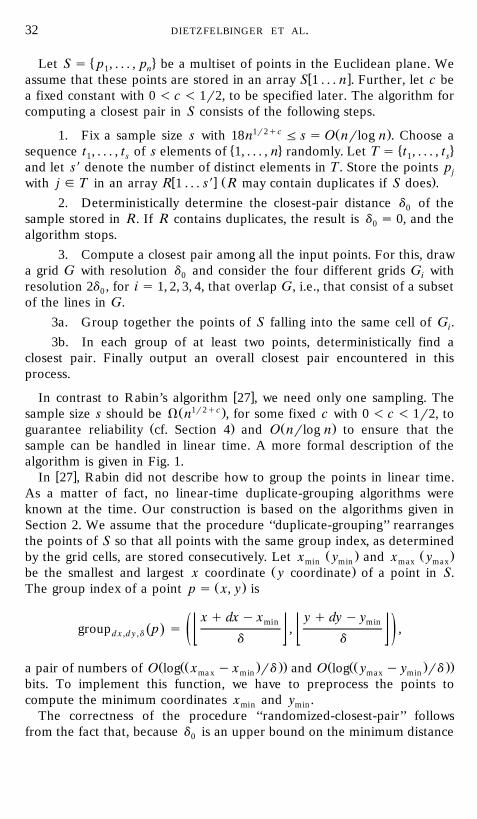
� 4Let S s p , . . . , p be a multiset of points in the Euclidean plane. We1 nw xassume that these points are stored in an array S 1 . . . n . Further, let c be
a fixed constant with 0 - c - 1r2, to be specified later. The algorithm forcomputing a closest pair in S consists of the following steps.
1r2qc Ž .1. Fix a sample size s with 18n F s s O nrlog n . Choose a� 4 � 4sequence t , . . . , t of s elements of 1, . . . , n randomly. Let T s t , . . . , t1 s 1 s
and let s9 denote the number of distinct elements in T. Store the points pjw x Ž .with j g T in an array R 1 . . . s9 R may contain duplicates if S does .
2. Deterministically determine the closest-pair distance d of the0sample stored in R. If R contains duplicates, the result is d s 0, and the0algorithm stops.
3. Compute a closest pair among all the input points. For this, drawa grid G with resolution d and consider the four different grids G with0 iresolution 2d , for i s 1, 2, 3, 4, that overlap G, i.e., that consist of a subset0of the lines in G.
3a. Group together the points of S falling into the same cell of G .i3b. In each group of at least two points, deterministically find a
closest pair. Finally output an overall closest pair encountered in thisprocess.
w xIn contrast to Rabin’s algorithm 27 , we need only one sampling. TheŽ 1r2qc.sample size s should be V n , for some fixed c with 0 - c - 1r2, to
Ž . Ž .guarantee reliability cf. Section 4 and O nrlog n to ensure that thesample can be handled in linear time. A more formal description of thealgorithm is given in Fig. 1.
w xIn 27 , Rabin did not describe how to group the points in linear time.As a matter of fact, no linear-time duplicate-grouping algorithms wereknown at the time. Our construction is based on the algorithms given inSection 2. We assume that the procedure ‘‘duplicate-grouping’’ rearrangesthe points of S so that all points with the same group index, as determined
Ž . Ž .by the grid cells, are stored consecutively. Let x y and x ymin min max maxŽ .be the smallest and largest x coordinate y coordinate of a point in S.
Ž .The group index of a point p s x, y is
x q dx y x y q dy y ymin mingroup p s , ,Ž .d x ,d y ,d ž /d d
Ž ŽŽ . .. Ž ŽŽ . ..a pair of numbers of O log x y x rd and O log y y y rdmax min max minbits. To implement this function, we have to preprocess the points tocompute the minimum coordinates x and y .min min
The correctness of the procedure ‘‘randomized-closest-pair’’ followsfrom the fact that, because d is an upper bound on the minimum distance0
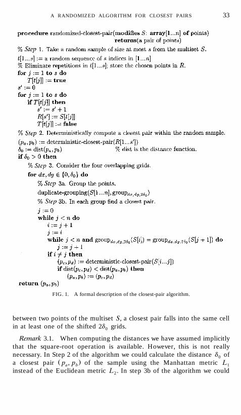
A RANDOMIZED ALGORITHM FOR CLOSEST PAIRS 33
FIG. 1. A formal description of the closest-pair algorithm.
between two points of the multiset S, a closest pair falls into the same cellin at least one of the shifted 2d grids.0
Remark 3.1. When computing the distances we have assumed implicitlythat the square-root operation is available. However, this is not reallynecessary. In Step 2 of the algorithm we could calculate the distance d of0
Ž .a closest pair p , p of the sample using the Manhattan metric La b 1instead of the Euclidean metric L . In step 3b of the algorithm we could2
DIETZFELBINGER ET AL.34
compare the squares of the L distances instead of the actual distances.2Whereas even with this change, d is an upper bound on the L distance0 2of a closest pair, the algorithm will still be correct. On the other hand, therunning-time estimate for step 3, as given in the next section, does not
Ž .change. See the analysis of step 3b following Corollary 4.4. The tricks justmentioned suffice to show that the closest-pair algorithm can be made towork for any fixed L metric without computing pth roots, if p is appositive integer or `.
Remark 3.2. The randomized closest-pair algorithm generalizes natu-Ž .rally to any d-dimensional space. Note that two shifts by 0 and d of 2d0 0
grids are needed in the one-dimensional case, in the two-dimensional case4 and in the d-dimensional case 2 d shifted grids must be taken intoaccount.
Remark 3.3. For implementing the procedure ‘‘deterministic-closest-pair’’ any of a number of algorithms can be used. Small input sets are besthandled by the ‘‘brute-force’’ algorithm, which calculated the distances
Ž .between all n n y 1 r2 pairs of points. In particular, all calls to‘‘deterministic-closest-pair’’ in step 3b are executed in this way. For largerinput sets, in particular, for the call to ‘‘deterministic-closest-pair’’ in step2, we use an asymptotically faster algorithm. For different numbers d ofdimensions various algorithms are available. In the one-dimensional casethe closest-pair problem can be solved by sorting the points and findingthe minimum distance between two consecutive points. In the two-dimensional case one can use the simple plane-sweep algorithm of
w xHinrichs et al. 17 . In the multidimensional case, the divide-and-conquerw xalgorithm of Bentley and Shamos 7 and the incremental algorithm of
w xSchwarz et al. 30 are applicable. Assuming d to be constant, all theŽ . Ž .algorithms mentioned previously run in O n log n time and O n space.
Be aware, however, that the complexity depends heavily on d.
4. ANALYSIS OF THE CLOSEST-PAIR ALGORITHM
In this section, we prove that the algorithm given in Section 3 has lineartime complexity with high probability. Again, we treat only the two-dimensional case in detail. Time bounds for most parts of the algorithmwere established in previous sections or are immediately clear: step 1 of
Ž . Ž .the algorithm taking the sample of size s9 F s obviously uses O s time.Ž . Ž .Whereas we assumed that s s O nrlog n , no more than O n time is
Žconsumed in step 2 for finding a closest pair within the sample see.Remark 3.3 . The complexity of the grouping performed in step 3a was
analyzed in Section 2. To implement the function group , whichd x,d y,d
A RANDOMIZED ALGORITHM FOR CLOSEST PAIRS 35
Ž .returns the group indices, we need some preprocessing that takes O ntime.
It remains only to analyze the cost of step 3b, where closest pairs arefound within each group. It will be shown that a sample of size s G
1r2qc Ž .18n , for any fixed c with 0 - c - 1r2, guarantees O n -time perfor-mance with a failure probability of at most 2yn c
. This holds even if aclosest pair within each group is computed by the brute-force algorithmŽ .see Remark 3.3 . On the other hand, if the sampling procedure ismodified in such a way that only a few fourwise independent sequences areused to generate the sampling indices t , . . . , t , linear running time will1 s
Ž ya .still be guaranteed with probability 1 y O n , for some constant a ,while the number of random bits needed is drastically reduced.
The analysis is complicated by the fact that points may occur repeatedly� 4in the multiset S s p , . . . , p . Of course, the algorithm will return two1 n
identical points p and p in this case, and the minimum distance is 0.a bw xNote that in Rabin’s paper 27 as well as in that of Khuller and Matias
w x19 , the input points are assumed to be distinct.w xAdapting a notion from 27 , we first define what it means that there are
‘‘many’’ duplicates and show that in this case the algorithm runs fast. Thelonger part of the analysis then deals with the situation where there arefew or no duplicate points. For reasons of convenience we will assumethroughout the analysis that n G 800.
Ž . Ž .For a finite multi set S and a partition D s S , . . . , S of S into1 mnonempty subsets, let
m1 < < < <N D s S ? S y 1 ,Ž . Ž .Ý m m2
ms1
Ž .which is the number of unordered pairs of elements of S that lie in thesame set S of the partition. In the case of the natural partition D of them S
� 4multiset S s p , . . . , p , where each class consists of all copies of one of1 nthe points, we use the abbreviation
� 4N S s N D s i , j N 1 F i - j F n and p s p .Ž . Ž . � 4S i j
Ž .We first consider the case where N S is large; more precisely, weŽ .assume for the time being that N S G n. In Appendix B it is proved that
'under this assumption, if we pick a sample of somewhat more than nrandom elements of S, with high probability the sample will contain atleast two equal points. More precisely, Corollary B.2 shows that thes G 18n1r2qc sample points chosen in step 1 of the algorithm will containtwo equal points with probability at least 1 y 2yn c
. The deterministicclosest-pair algorithm invoked in step 2 will identify one such pair of
DIETZFELBINGER ET AL.36
duplicates and return d s 0; at this point the algorithm terminates,0having used only linear time.
For the remainder of this section we assume that there are not too manyŽ .duplicate points, that is, that N S - n. In this case, we may follow the
argument from Rabin’s paper. If G is a grid in the plane, then G induces aŽpartition D of the multiset S into disjoint subsets S , . . . , S withS,G 1 m
.duplicates . Two points of S are in the same subset of the partition if andonly if they fall into the same cell of G. As in the preceding special case ofŽ .N S , we are interested in the number
N S, G s N DŽ . Ž .S ,G
� 4s i , j N p and p lie in the same cell of the grid G .� 4i j
w xThis notion, which was also used in Rabin’s analysis 27 , expresses thework done in step 3b when the subproblems are solved by the brute-forcealgorithm.
w xLEMMA 4.1 27 . Let S be a multiset of n points in the plane. Further, letG be a grid with resolution d and let G9 be one of the four grids with
3Ž . Ž .resolution 2d that o¨erlap G. Then N S, G9 F 4N S, G q n.2
Proof. We consider four cells of G whose union is one cell of G9.Assume that these four cells contain k , k , k , and k points from S1 2 3 4Ž . Ž .with duplicates , respectively. The contribution of these cells to N S, G is
1 4 Ž . Ž . Ž .b s Ý k k y 1 . The contribution of the one larger cell to N S, G9is1 i i21 4Ž .is k k y 1 , where k s Ý k . We want to give an upper bound onis1 i2
1 Ž .k k y 1 in terms of b.2Ž . w .The function x ¬ x x y 1 is convex in 0, ` . Hence
41 1 1 1k k y 1 F k k y 1 s b.Ž .Ž . Ý i i4 4 4 2
is1
This implies
1 1 3 1 1 3 3k k y 1 s k k y 4 q k F 8 ? k k y 1 q k F 4 ? b q k .Ž . Ž . Ž .2 2 2 4 4 2 2
Summing the last inequality over all cells of G9 yields the desired inequal-3Ž . Ž .ity N S, G9 F 4N S, G q n.2
Remark 4.2. In the case of d-dimensional space, this calculationcan be carried out in exactly the same way. This results in the estimate
1d dŽ . Ž . Ž .N S, G9 F 2 N S, G q 2 y 1 n.2
Ž .COROLLARY 4.3. Let S be a multiset of n points that satisfies N S - n.Ž .Then there is a grid G* with n F N S, G* - 5.5n.
A RANDOMIZED ALGORITHM FOR CLOSEST PAIRS 37
Proof. We start with a grid G so fine that no cell of the grid containsŽ . Ž .two distinct points in S. Then, obviously, N S, G s N S - n. By repeat-
Ž .edly doubling the grid size as in Lemma 4.1 until N S, G9 G n for the firsttime, we find a grid G* satisfying the claim.
COROLLARY 4.4. Let S be a multiset of size n and let G be a grid withresolution d . Further, let G9 be an arbitrary grid with resolution at most d .
Ž . Ž .Then N S, G9 F 16N S, G q 6n.
Proof. Let G , for i s 1, 2, 3, 4, be the four different grids with resolu-i
tion 2d that overlap G. Each cell of G9 is completely contained in somecell of at least one of the grids G . Thus, the sets of the partition inducedi
by G9 can be divided into four disjoint classes depending on which of thegrids G covers the corresponding cell completely. Therefore, we haveiŽ . 4 Ž .N S, G9 F Ý N S, G . Applying Lemma 4.1 and summing up yieldsis1 iŽ . Ž .N S, G9 F 16N S, G q 6n, as desired.
Now we are ready to analyze step 3b of the algorithm. As previouslyŽ .stated, we assume that N S - n; hence the existence of some grid G* as
in Corollary 4.3 is ensured. Let d * ) 0 denote the resolution of G*.Ž .We apply Corollary B.2 to the partition of S with duplicates induced by
G* to conclude that with probability at least 1 y 2yn cthe random sample
taken in step 1 of the algorithm contains two points from the same cell ofG*. It remains to show that if this is the case, then step 3b of the algorithm
Ž .takes O n time.Whereas the real number d calculated by the algorithm in step 2 is0
bounded by the distance of two points in the same cell of G*, we mustŽhave d F 2d *. This is the case even if in step 2 the Manhattan metric L0 1
.is used. Thus the four grids G , G , G , G used in step 3 have resolution1 2 3 42d F 4d *. We form a new conceptual grid G** with resolution 4d * by0
Ž .omitting all but every fourth line from G*. By the inequality N S, G* -Ž .5.5n Corollary 4.3 and a double application of Lemma 4.1, we obtain
Ž . Ž .N S, G** s O n . The resolution 4d * of the grid G** is at least 2d .0Hence we may apply Corollary 4.4 to obtain that the four grids
Ž . Ž .G , G , G , G used in step 3 of the algorithm satisfy N S, G s O n , for1 2 3 4 iŽ 4 Ž Ž .i s 1, 2, 3, 4. Obviously the running time of step 3b is O Ý N S, G qis1 i
..n ; by the foregoing statement this bound is linear in n. This finishes theanalysis of the cost of step 3b.
It is easy to see that Corollaries 4.3 and 4.4 as well as the analysis of step3b generalize from the plane to any fixed dimension d. Combining thepreceding discussion with Theorem 2.13, we obtain the following theorem.
DIETZFELBINGER ET AL.38
THEOREM 4.5. The closest-pair problem for a multiset of n points ind-dimensional space, where d G 1 is a fixed integer, can be sol ed by a
Ž .randomized algorithm that needs O n space and
Ž . Ž . �1 O n time on a real RAM with operations from q, y, ), DIV,4LOG , EXP or2 2
Ž . Ž Ž ..2 O n q log log d rd time on a real RAM with operationsmax min� 4from q, y, ), DIV ,
where d and d denote the maximum and the minimum distance betweenmax minany two distinct points, respecti ely. The probability that the time bound isexceeded is 2yn V Ž1.
.
Proof. The running time of the randomized closest-pair algorithm isdominated by that of step 3a. The group indices used in step 3a are
� u v4d-tuples of integers in the range 0, . . . , d rd . By Theorem 2.14,max minŽ . Ž .parts 1 and 2 of the theorem follow directly from the corresponding
parts of Theorem 2.13. Whereas all the subroutines used finish within theirrespective time bounds with probability 1 y 2yn V Ž1.
, the same is true forthe whole algorithm. The amount of space required is obviously linear.
In the situation of Theorem 4.5, if the coordinates of the input points� 4happen to be integers drawn from a range 0, . . . , U y 1 , we can replace
the real RAM by a conservative unit-cost RAM with integer operations;Ž . Ž .the time bound of part 2 then becomes O n q log log U . The number of
random bits used by either version of the algorithm is quite large, namely,essentially as large as possible with the given running time. Even if thenumber of random bits used is severely restricted, we can still retain analgorithm that is polynomially reliable.
THEOREM 4.6. Let a , d G 1 be arbitrary fixed integers. The closest-pairproblem for a multiset of n points in d-dimensional space can be sol ed by arandomized algorithm with the time and space requirements stated in Theorem
Ž Ž .. w Ž4.5 that uses only O log n q log d rd random bits or O log n qmax min. � 4xlog U random bits for integer input coordinates in the range 0, . . . , U y 1
Ž ya .and that exceeds the time bound with probability O n .
u 3r4 vProof. We let s s 16a ? n and generate the sequence t , . . . , t in1 sthe algorithm as the concatenation of 4a independently chosen sequencesof four-independent random values that are approximately uniformly dis-
� 4tributed in 1, . . . , n . This random experiment and its properties aredescribed in detail in Corollary B.4 and Lemma B.5 in Appendix B. The
Ž . Ž .time needed is o n , and the number of random bits needed is O log n .The duplicate grouping is performed with the simple method described in
Ž Ž .. Ž .Section 2.3. This requires only O log d rd or O log U random bits.max min
A RANDOMIZED ALGORITHM FOR CLOSEST PAIRS 39
The analysis is exactly the same as in the proof of Theorem 4.5, except thatCorollary B.4 is used instead of Corollary B.2.
5. CONCLUSIONS
We have provided an asymptotically efficient algorithm for computing aclosest pair of n points in d-dimensional space. The main idea of thealgorithm is to use random sampling to reduce the original problem to acollection of duplicate-grouping problems. The performance of the algo-rithm depends on the operations assumed to be primitive in the underlyingmachine model. We proved that, with high probability, the running time
Ž .is O n on a real RAM capable of executing the arithmetic operations� 4from q, y, ), DIV, LOG , EXP in constant time. Without the operations2 2
LOG and EXP , the running time increases by an additive term of2 2Ž Ž ..O log log d rd , where d and d denote the maximum andmax min max min
the minimum distance between two distinct points, respectively. When the� 4coordinates of the points are integers in the range 0, . . . , U y 1 , the
Ž . Ž .running times are O n and O n q log log U , respectively. For integerdata the algorithm is conservative, i.e., all the numbers manipulated
Ž .contain O log n q log U bits.We proved that the bounds on the running times hold also when the
collection of input points contains duplicates. As an immediate corollary ofthis result we get that the following decision problems, which are often
Ž w x.used in lower-bound arguments for geometric problems see 26 , can besolved as efficiently as the one-dimensional closest-pair problem on the
Ž .real RAM Theorems 4.5 and 4.6 :Ž .1 Element-distinctness problem: Given n real numbers, decide if
any two of the numbers are equal.Ž .2 «-closeness problem: Given n real numbers and a threshold value
« ) 0, decide if any two of the numbers are at distance less than « fromeach other.
Finally, we would like to mention practical experiments with our simpleduplicate-grouping algorithm. The experiments were concluded by Tomi
Ž .Pasanen University of Turku, Finland . He found that the duplicate-grouping algorithm described in Theorem 2.7, which is based on radix sortŽ .with a s 3 , behaves essentially as well as heap sort. For small inputsŽ .n - 50,000 , heap sort was slightly faster, whereas for large inputs, heapsort was slightly slower. Randomized quick sort turned out to be muchfaster than any of these algorithms for all n F 1,000,000. One drawback ofthe radix-sort algorithm is that it requires extra memory space for linking
DIETZFELBINGER ET AL.40
Ž .the duplicates, whereas heap sort as well as in-place quick sort does notrequire any extra space. One should also note that in some applicationsthe word length of the actual machine can be restricted to, say, 32 bits.
11 ŽThis means that when n ) 2 and a s 3, the hash function h g HH seek ,l.the proof of Theorem 2.7 is not needed for collapsing the universe; radix
sort can be applied directly. Therefore the integers must be long beforethe full power of our methods comes into play.
APPENDIX A. GENERATING PRIMES
In this appendix we provide a proof of Lemma 2.9. The main idea isexpressed in the proof of the following lemma.
LEMMA A.1. There is a randomized algorithm that, for any gi en integerm G 2, returns an integer p with m - p F 2m such that the following
ŽŽ .4.statement holds: the running time is O log m and the probability that p isnot prime is at most 1rm.
Proof. The heart of the construction is the randomized primality testw x w x Ždue to Miller 25 and Rabin 28 for a description and an analysis, see,
w x.e.g., 10, p. 839ff . If an arbitrary number x of b bits is given to the test asan input, then the following holds:
Ž . Ž .1 If x is prime, then Prob the result of the test is ‘‘prime’’ s 1.Ž . Ž .2 If x is composite, then Prob the result of the test is ‘‘prime’’ F
1r4.Ž . Ž .3 Performing the test once requires O b time and all numbers
Ž .manipulated in the test are O b bits long.
By repeating the test t times, the reliability of the result can be increasedsuch that for composite x we have
Prob the result of the test is ‘‘prime’’ F 1r4 t .Ž .
To generate a ‘‘probable prime’’ that is greater than m we use a randomŽ .sampling algorithm. We select s to be specified later integers from the
� 4interval m q 1, . . . , 2m at random. Then these numbers are tested one byone until the result of the test is ‘‘prime.’’ If no such result is obtained, thenumber m q 1 is returned.
The algorithm fails to return a prime number if there is no prime amongthe numbers in the sample or if one of the composite numbers in thesample is accepted by the primality test. Next we estimate the probabilitiesof these events.
A RANDOMIZED ALGORITHM FOR CLOSEST PAIRS 41
Ž . <� 4 <It is known that the function p x s p N p F x and p is prime ,defined for any real number x, satisfies
np 2n y p n )Ž . Ž .
3 ln 2nŽ .Žfor all integers n ) 1. For a complete proof of this fact, also known as the
w x .inequality of Finsler, see 31, Sects. 3.10 and 3.14 . That is, the number of� 4 Ž Ž ..primes in the set m q 1, . . . , 2m is at least mr 3 ln 2m . We choose
2s s s m s 3 ln 2mŽ . Ž .Ž .and
t s t m s max log s m , log 2m .� 4Ž . Ž . Ž .2 2
w Ž . Ž . xNote that t m s O log m . Then the probability that the random samplecontains no prime at all is bounded by
Ž .ln 2 ms Ž .3 ln 2 m1 1 1ln Ž2 m.1 y F 1 y - e s .ž / ž /ž /3 ln 2m 3 ln 2m 2mŽ . Ž .
The probability that one of the at most s composite numbers in the samplewill be accepted is smaller than
1t ylog sŽm. ylog Ž2 m.2 2s m ? 1r4 F s m ? 2 ? 2 s .Ž . Ž . Ž .2m
Summing up, the failure probability of the algorithm is at mostŽ Ž ..2 ? 1r 2m s 1rm, as claimed. If m is a b-bit number, the time required
4Ž . ŽŽ . .is O s ? t ? b , that is, O log m .
Remark A.2. The problem of generating primes is discussed in greaterw xdetail by Damgard et al. 11 . Their analysis shows that the proof of˚
Lemma A.1 is overly pessimistic. Therefore, without sacrificing reliability,the sample size s andror the repetition count t can be decreased; in thisway considerable savings in the running time are possible.
LEMMA 2.9. There is a randomized algorithm that, for any gi en positi eintegers m and n with 2 F m F 2 u n1r4 v, returns a number p with m - p F 2m
Ž .such that the following statement holds: the running time is O n , and theprobability that p is not prime is at most 2yn1r4
.
Proof. We increase the sample size s and the repetition count t in thealgorithm of Lemma A.1 as
1r4s s s m , n s 6 ? ln 2m ? nŽ . Ž . u v
and1r4t s t m , n s 1 q max log s m , n , n .Ž . Ž . u v� 42
DIETZFELBINGER ET AL.42
As before, the failure probability is bounded by the sum of the terms
Ž .s m , n1 1r4 1r4y2 u n v y1yn1 y - e - 2ž /3 ln 2mŽ .
and
Ž . 1r4 1r4t m , n yŽ1qu n v. y1yns m , n ? 1r4 F 2 F 2 .Ž . Ž .
This proves the bound 2yn1r4on the failure probability. The running time
is
O s ? t ? log m s O log m ? n1r4 ? log log m q log n q n1r4 ? log mŽ . Ž . Ž .Ž .s O n .Ž .
APPENDIX B. RANDOM SAMPLING IN PARTITIONS
In this appendix we deal with some technical details of the analysis ofthe closest-pair algorithm. For a finite set S and a partition D sŽ .S , . . . , S of S into nonempty subsets, let1 m
< < � 4P D s p : S N p s 2 n 'm g 1, . . . , m : p : S .Ž . � 4m
Ž . < Ž . <Note that the quantity N D defined in Section 4 equals P D . For theanalysis of the closest-pair algorithm, we need the following technical fact:
'Ž .If N D is linear in n and more than 8 n elements are chosen at randomfrom S, then with a probability that is not too small, two elements fromthe same subset of the partition are picked. A similar lemma was proved
w xby Rabin 27, Lemma 6 . In Appendix B.1 we give a totally different proof,Ž .resting on basic facts from probability theory viz., Chebyshev’s inequality ,
which may make it more obvious than Rabin’s proof why the lemma istrue. Further, it will turn out that full independence of the elements in therandom sample is not needed, but rather that fourwise independence issufficient. This observation is crucial for a version of the closest-pairalgorithm that uses only few random bits. The technical details are given inAppendix B.2.
B.1. The sampling lemma
LEMMA B.1. Let n, m, and s be positi e integers, let S be a set of sizeŽ .n G 800, let D s S , . . . , S be a partition of S into nonempty subsets with1 m
A RANDOMIZED ALGORITHM FOR CLOSEST PAIRS 43
Ž .N D G n, and assume that s random elements t , . . . , t are drawn indepen-1 s 'dently from the uniform distribution o¨er S. Then if s G 8 n ,
� 4 � 4Prob ' i , j g 1, . . . , s 'm g 1, . . . , m : t / t n t , t g SŽ .i j i j m
'4 n) 1 y . B.1Ž .
s
Proof. We first note that we may assume, without loss of generality,that
n F N D F 1.1n. B.2Ž . Ž .
Ž .To see this, assume that N D ) 1.1n and consider a process of repeat-edly refining D by splitting off an element x in a largest set in D, i.e., by
'making x into a singleton set. As long as D contains a set of size 2n q 2Ž .or more, the resulting partition D9 still has N D9 G n. On the other
'hand, splitting off an element from a set of size less than 2n q 2 changes' 'N by less than 2n q 1 s 200rn ? 0.1n q 1, which for n G 800 is at
most 0.1n. Hence if we stop the process with the first partition D9 withŽ . Ž .N D9 F 1.1n, we will still have N D9 G n. Whereas D9 is a refinement
of D, we have for all i and j that
t and t are contained in the same set SX of D9i j m
« t and t are contained in the same set S of D ;i j m
Ž .thus, it suffices to prove B.1 for D9.p Ž .We define random variables X , for p g P D and 1 F i - j F s, asi, j
1 if t , t s p ,� 4i jpX si , j ½ 0 otherwise.
Further, we let
X s Xp .Ý Ý i , jŽ . 1Fi-jFspgP D
Ž .Clearly, by the definition of P D ,
X s i , j N 1 F i - j F s n t / t n t , t g S for some m G 0.Ž .� 4i j i j m
Ž .Thus, to establish B.1 , we only have to show that
'4 nProb X s 0 - .Ž .
s
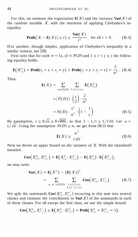
DIETZFELBINGER ET AL.44
Ž . Ž .For this, we estimate the expectation E X and the variance Var X ofthe random variable X, with the intention of applying Chebyshev’s in-equality:
Var XŽ .Prob X y E X G t F for all t ) 0. B.3Ž . Ž .Ž . 2t
ŽFor another, though simpler, application of Chebyshev’s inequality in aw x.similar context, see 9 .
� 4 Ž .First note that for each p s x, y g P D and 1 F i - j F s the follow-ing equality holds:
2pE X s Prob t s x n t s y q Prob t s y n t s x s . B.4Ž .Ž . Ž .Ž .i , j i j i j 2n
Thus,
E X s E XpŽ . Ž .Ý Ý i , jŽ . 1Fi-jFspgP D
2ss P D ? ?Ž . 2ž /2 n
s2 1s N D ? ? 1 y . B.5Ž . Ž .2 ž /sn
' 'By assumption, s G 8 n G 8 800 , so that 1 y 1rs G 1r1.01. Let a s' Ž . Ž .sr n . Using the assumption N D G n, we get from B.5 that
a 2
E X G . B.6Ž . Ž .1.01
Ž .Next we derive an upper bound on the variance of X. With the standardnotation
Cov Xp , Xp 9 s E Xp ? Xp 9 y E Xp ? E Xp 9 ,Ž .Ž . Ž . Ž .i , j i9 , j9 i , j i9 , j9 i , j i9 , j9
we may write22Var X s E X y E XŽ . Ž . Ž .Ž .
s Cov Xp , Xp 9 . B.7Ž .Ž .Ý Ý i , j i9 , j9Ž . 1Fi-jFsp , p 9gP D
1Fi9-j9Fs
Ž p p 9 .We split the summands Cov X , X occurring in this sum into severali, j i9, j9Ž .classes and estimate the contribution to Var X of the summands in each
of these classes. For all except the first class, we use the simple bound
Cov Xp , Xp 9 F E Xp ? Xp 9 s Prob Xp s Xp 9 s 1 .Ž . Ž . Ž .i , j i9 , j9 i , j i9 , j9 i , j i9 , j9
A RANDOMIZED ALGORITHM FOR CLOSEST PAIRS 45
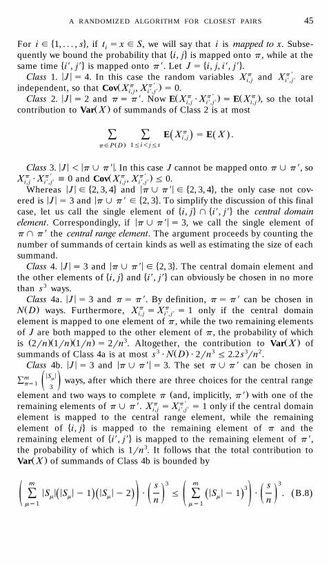
� 4For i g 1, . . . , s , if t s x g S, we will say that i is mapped to x. Subse-i� 4quently we bound the probability that i, j is mapped onto p , while at the
� 4 � 4same time i9, j9 is mapped onto p 9. Let J s i, j, i9, j9 .< < p p 9Class 1. J s 4. In this case the random variables X and X arei, j i9, j9
Ž p p 9 .independent, so that Cov X , X s 0.i, j i9, j9< < Ž p p 9 . Ž p .Class 2. J s 2 and p s p 9. Now E X ? X s E X , so the totali, j i9, j9 i, j
Ž .contribution to Var X of summands of Class 2 is at most
E Xp s E X .Ž .Ž .Ý Ý i , jŽ . 1Fi-jFspgP D
< < < <Class 3. J - p j p 9 . In this case J cannot be mapped onto p j p 9, sop p 9 Ž p p 9 .X ? X ' 0 and Cov X , X F 0.i, j i9, j9 i, j i9, j9
< < � 4 < < � 4Whereas J g 2, 3, 4 and p j p 9 g 2, 3, 4 , the only case not cov-< < < � 4ered is J s 3 and p j p 9 g 2, 3 . To simplify the discussion of this final
� 4 � 4case, let us call the single element of i, j l i9, j9 the central domain< <element. Correspondingly, if p j p 9 s 3, we call the single element of
p l p 9 the central range element. The argument proceeds by counting thenumber of summands of certain kinds as well as estimating the size of eachsummand.
< < < < � 4Class 4. J s 3 and p j p 9 g 2, 3 . The central domain element and� 4 � 4the other elements of i, j and i9, j9 can obviously be chosen in no more
than s3 ways.< <Class 4a. J s 3 and p s p 9. By definition, p s p 9 can be chosen in
Ž . p pN D ways. Furthermore, X s X s 1 only if the central domaini, j i9, j9element is mapped to one element of p , while the two remaining elementsof J are both mapped to the other element of p , the probability of which
Ž .Ž .Ž . 3 Ž .is 2rn 1rn 1rn s 2rn . Altogether, the contribution to Var X of3 Ž . 3 3 2summands of Class 4a is at most s ? N D ? 2rn F 2.2 s rn .
< < < <Class 4b. J s 3 and p j p 9 s 3. The set p j p 9 can be chosen in< <Sm mÝ ways, after which there are three choices for the central rangeps1 ž /3
Ž .element and two ways to complete p and, implicitly, p 9 with one of theremaining elements of p j p 9. Xp s Xp 9 s 1 only if the central domaini, j i9, j9element is mapped to the central range element, while the remaining
� 4element of i, j is mapped to the remaining element of p and the� 4remaining element of i9, j9 is mapped to the remaining element of p 9,
the probability of which is 1rn3. It follows that the total contribution toŽ .Var X of summands of Class 4b is bounded by
m m3 3s s3< < < < < < < <S S y 1 S y 2 ? F S y 1 ? . B.8Ž .Ž . Ž . Ž .Ý Ým m m mž / ž /ž / ž /n nms1 ms1
DIETZFELBINGER ET AL.46
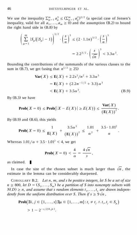
m 3 Ž m 2 .3r2 ŽWe use the inequality Ý a F Ý a a special case of Jensen’sms1 m ms1 m
. Ž .inequality, valid for all a , . . . , a G 0 and the assumption B.2 to bound1 mŽ .the right hand side in B.8 by
3r2m 3 3s s3r2< < < <S S y 1 ? F 2 ? 1.1n ?Ž .Ž .Ý m m ž / ž /ž / n nms1
3s3r2 3s 2.2 ? - 3.3a .ž /'n
Bounding the contributions of the summands of the various classes to theŽ . Ž 1r2 .sum in B.7 , we get using that n G 25
Var X F E X q 2.2 s3rn2 q 3.3a 3Ž . Ž .s E X q 2.2ny1r2 q 3.3 a 3Ž . Ž .- E X q 3.5a 3. B.9Ž . Ž .
Ž .By B.3 we have
Var XŽ .Prob X s 0 F Prob X y E X G E X F .Ž . Ž . Ž .Ž . 2E XŽ .Ž .
Ž . Ž .By B.9 and B.6 , this yields
1 3.5a 3 1.01 3.5 ? 1.012
Prob X s 0 F q F q .Ž . 2 2E X aaŽ . E XŽ .Ž .
Whereas 1.01ra q 3.5 ? 1.012 - 4, we get
'4 4 nProb X s 0 - s ,Ž .
a s
as claimed.
'In case the size of the chosen subset is much larger than n , theestimate in the lemma can be considerably sharpened.
COROLLARY B.2. Let n, m, and s be positi e integers, let S be a set of sizeŽ .n G 800, let D s S , . . . , S be a partition of S into nonempty subsets with1 m
Ž .N D G n, and assume that s random elements t , . . . , t are drawn indepen-1 s 'dently from the uniform distribution o¨er S. Then if s G 9 n ,
� 4 � 4Prob ' i , j g 1, . . . , s 'm g 1, . . . , m : t / t n t , t g SŽ .i j i j m
.ysrŽ18 n') 1 y 2 .
A RANDOMIZED ALGORITHM FOR CLOSEST PAIRS 47
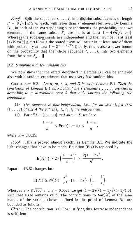
Proof. Split the sequence t , . . . , t into disjoint subsequences of length1 s' 'u vs9 s 8 n F 9 n each, with fewer than s9 elements left over. By LemmaB.1, in each of the corresponding subexperiments the probability that two
1'elements in the same subset S are hit is at least 1 y 4 n rs9 G .m 2
Whereas the subexperiments are independent and their number is at least' '? Ž .@ Ž .sr 9 n G sr 18 n , the stated event will occur in at least one of them
ys rŽ18 n .'with probability at least 1 y 2 . Clearly, this is also a lower boundon the probability that the whole sequence t , . . . , t hits two elements1 sfrom the same S .m
B.2. Sampling with few random bits
We now show that the effect described in Lemma B.1 can be achievedalso with a random experiment that uses very few random bits.
COROLLARY B.3. Let n, m, s, S, and D be as in Lemma B.1. Then theconclusion of Lemma B.1 also holds if the s elements t , . . . , t are chosen1 saccording to a distribution o¨er S that only satisfies the following twoconditions:
Ž . � 41 The sequence is four-independent, i.e., for all sets i, j, k, l :� 41, . . . , s of size 4 the ¨alues t , t , t , t are independent.i j k l
Ž . � 42 For all i g 1, . . . , s and all x g S, we ha¨e
1 y « 1 q «- Prob t s x - ,Ž .in n
where « s 0.0025.
Proof. This is proved almost exactly as Lemma B.1. We indicate theŽ .light changes that have to be made. Equation B.4 is replaced by
21 y « 2 1 y 2«Ž .pE X G 2 ? G .Ž .i , j 2ž /n n
Ž .Equation B.5 changes into
s2 1E X G N D ? ? 1 y 2« ? 1 y .Ž . Ž . Ž .2 ž /sn
' Ž .Ž .Whereas s G 8 800 and « s 0.0025, we get 1 y 2« 1 y 1rs G 1r1.01,Ž . Ž .such that B.6 remains valid. The contributions to Var X of the sum-
mands of the various classes defined in the proof of Lemma B.1 arebounded as follows.
Class 1. The contribution is 0. For justifying this, fourwise independenceis sufficient.

DIETZFELBINGER ET AL.48
Ž .Class 2. E X .Class 3. F0.
3 Ž . Ž 3. Ž .3 3 2Class 4a. s ? N D ? 2rn ? 1 q « F 2.3s rn .Ž .3r2 Ž 3. Ž .3 3Class 4b. 2.2n ? srn ? 1 q « F 3.3a .
Ž .Finally, estimate B.9 is replaced by
Var x F E X q 2.3ny1r2 q 3.3 a 3 - E X q 3.5a 3 ,Ž . Ž . Ž . Ž .
where we used that n1r2 G 25. The rest of the argument is verbally thesame as in the proof of Lemma B.1.
In the random sampling experiment, we can even achieve polynomialreliability with a moderate number of random bits.
u 3r4 vCOROLLARY B.4. In the situation of Lemma B.1, let s G 4 n and leta G 1 be an arbitrary integer. If the experiment described in Corollary B.3 is
Ž .repeated independently 4a times to generate 4a sequences t , . . . , t , withl,1 l, s1 F l F 4a , of elements of S, then
� 4 � 4 � 4Prob 'k , l g 1, . . . , 4a ' i , j g 1, . . . , s 'm g 1, . . . , m :Žt / t n t , t g S ) 1 y nya ..k ,i l , j k ,i l , j m
Proof. By Corollary B.3, for each fixed l the probability that thesequence t , . . . , t hits two different elements in the same subset S is atl,1 l, s m
y1r4'least 1 y 4 nrs G 1 y n . By independence, the probability that thisŽ y1r4.4ahappens for one of the 4a sequences is at least 1 y n . Clearly,
this is also a lower bound on the probability that the whole sequence t ,l,iwith 1 F l F 4a and 1 F i F s, hits two different elements in the sameset S .m
� 4 u 3r4 vLEMMA B.5. Let S s 1, . . . , n for some n G 800 and take s s 4 n .Then the random experiment described in Corollary B.3 can be carried out
Ž . Ž 6. win o n time using a sample space of size O n or, informally, usingŽ . x6 log n q O 1 random bits .2
Proof. Let us assume for the time being that a prime number p withŽs - p F 2 s is given. We will see at the end of the proof how such a prime
. w xcan be found within the time bound claimed. According to 9 , a four-in-dependent sequence tX , . . . , tX , where each tX is uniformly distributed in1 p j� 4 X0, . . . , p y 1 , can be generated as follows: Choose four coefficients g ,0
X X X � 4g , g , g randomly from 0, . . . , p y 1 and let1 2 3
3X X rt s g ? j mod p for 1 F j F p.Ýj rž /
rs0
A RANDOMIZED ALGORITHM FOR CLOSEST PAIRS 49
Ž .By repeating this experiment once independently , we obtain another suchsequence tY, . . . , tY . We let1 p
t s 1 q tX q ptY mod n for 1 F j F s.Ž .j j j
Ž 4.2 8 Ž 6.Clearly, the overall size of the sample space is p s p s O n , andŽ .the time needed for generating the sample is O s . We must show that the
Ž . Ž .distribution of t , . . . , t satisfies conditions 1 and 2 of Corollary B.3.1 sŽ X X . Ž Y Y .Whereas the two sequences t , . . . , t and t , . . . , t originate from1 p 1 p
independent experiments and each of them is four-independent, thesequence
tX q ptY , . . . , tX q ptY1 1 s s
Ž .is four-independent; hence the same is true for t , . . . , t , and 1 is proved.1 sX Y � 2 4Further, t q pt is uniformly distributed in 0, . . . , p y 1 , for 1 F j F s.j j
From this, it is easily seen that, for x g S,
2 2p 1 p 1Prob t s x g ? , ? .Ž .j 2 2½ 5n np p
? 2 @ 2 u 2 v 2Now observe that p rn rp - 1rn - p rn rp and that
2 2p 1 p 1 1 1 1 1 1 «? y ? F - F s ? - ,2 2 2 2 3r2 'n n n np p p s 16n 16 n
'Ž .where we used that n G 800, whence 1r 16 n - 1r400 s 0.0025 s « .Ž .This proves 2 .
Finally, we briefly recall the fact that a prime number in the range� 4 Ž . Žs q 1, . . . , 2 s can be found deterministically in time O s log log s . Notethat we should not use randomization here, because we must take care not
.to use too many random bits. The straightforward implementation of theŽ w x.Eratosthenes sieve see, e.g., 31, Sect. 3.2 for finding all the primes in
� 41, . . . , 2 s has running time
1O s q 2 srp s O s ? 1 q s O s log log s ,u v Ž .Ý Ýž / p� 0� 0' 'pF 2 s pF 2 s
p prime p prime
where the last estimate results from the fact that
1s O log log x .Ž .Ý ppFx
p prime
DIETZFELBINGER ET AL.50
Ž Ž .For instance, this can easily be derived from the inequality p 2n yŽ . Ž . wp n - 7nr 5 ln n , valid for all integers n ) 1, which is proved in 31,
x .Sect. 3.14 .
ACKNOWLEDGMENTS
We thank Ivan Damgard for his comments concerning Lemma A.1 and Tomi Pasanen for˚his assistance in evaluating the practical efficiency of the duplicate-grouping algorithm. Thequestion of whether the class of multiplicative hash functions is universal was posed to thefirst author by Ferri Abolhassan and Jorg Keller. We also thank Kurt Mehlhorn for useful¨comments on this universal class and on the issue of four-independent sampling.
REFERENCES
1. A. Aggarwal, H. Edelsbrunner, P. Raghavan, and P. Tiwari, Optimal time bounds forŽ .some proximity problems in the plane, Inform. Process. Lett. 42 1992 , 55]60.
2. A. V. Aho, J. E. Hopcroft, and J. D. Ullman, ‘‘The Design and Analysis of ComputerAlgorithms,’’ Addison-Wesley, Reading, 1974.
3. A. Andersson, T. Hagerup, S. Nilsson, and R. Raman, Sorting in linear time?, in‘‘Proceedings of the 27th Annual ACM Symposium on the Theory of Computing,’’ ACMPress, New York, 1995, pp. 427]436.
4. H. Bast and T. Hagerup, Fast and reliable parallel hashing, in ‘‘Proceedings of the 3rdAnnual ACM Symposium on Parallel Algorithms and Architectures,’’ ACM Press, NewYork, 1991, pp. 50]61.
5. P. Beauchemin, G. Brassard, C. Crepeau, C. Goutier, and C. Pomerance, The generation´Ž .of random numbers that are probably prime, J. Cryptology 1 1988 , 53]64.
6. M. Ben-Or, Lower bounds for algebraic computation trees, in ‘‘Proceedings of the 15thAnnual ACM Symposium on Theory of Computing,’’ ACM Press, New York, 1983,pp. 80]86.
7. J. L. Bentley and M. I. Shamos, Divide-and-conquer in multidimensional space, in‘‘Proceedings of the 8th Annual ACM Symposium on Theory of Computing,’’ ACM Press,New York, 1976, pp. 220]230.
8. J. L. Carter and M. N. Wegman, Universal classes of hash functions, J. Comput. SystemŽ .Sci. 18 1979 , 143]154.
9. B. Chor and O. Goldreich, On the power of two-point based sampling, J. Complexity 5Ž .1989 , 96]106.
10. T. H. Cormen, C. E. Leiserson, and R. L. Rivest, ‘‘Introduction to Algorithms,’’ The MITPress, Cambridge, 1990.
11. I. Damgard, P. Landrock, and C. Pomerance, Average case error estimates for the strong˚Ž .probable prime test, Math. Comp. 61 1993 , 177]194.
12. M. Dietzfelbinger, A. Karlin, K. Mehlhorn, F. Meyer auf der Heide, H. Rohnert, andR. E. Tarjan, Dynamic perfect hashing: Upper and lower bounds, SIAM J. Comput. 23Ž .1994 , 738]761.
13. M. Dietzfelbinger and F. Meyer auf der Heide, Dynamic hashing in real time, inŽ‘‘Informatik}Festschrift zum 60 Geburtstag von Gunter Hotz’’ J. Buchmann, H.¨
.Ganzinger, and W. J. Paul, Eds. , Teubner-Texte zur Informatik, Vol. 1, Teubner,Stuttgart, 1992, pp. 95]119.
A RANDOMIZED ALGORITHM FOR CLOSEST PAIRS 51
Ž .14. M. L. Fredman, J. Komlos, and E. Szemeredi, Storing a sparse table with O 1 worst case´ ´Ž .access time, J. ACM 31 1984 , 538]544.
15. S. Fortune and J. Hopcroft, A note on Rabin’s nearest-neighbor algorithm, Inform.Ž .Process. Lett. 8 1979 , 20]23.
16. M. Golin, R. Raman, C. Schwarz, and M. Smid, Simple randomized algorithms for closestŽ .pair problems, Nordic J. Comput. 2 1995 , 3]27.
17. K. Hinrichs, J. Nievergelt, and P. Schorn, Plane-sweep solves the closest pair problemŽ .elegantly, Inform. Process. Lett. 26 1988 , 255]261.
18. J. Katajainen and M. Lykke, ‘‘Experiments with Universal Hashing,’’ Technical Report96r8, Dept. of Computer Science, Univ. of Copenhagen, Copenhagen, 1996.
19. S. Khuller and Y. Matias, A simple randomized sieve algorithm for the closest-pairŽ .problem, Inform. Comput. 118 1995 , 34]37.
20. D. Kirkpatrick and S. Reisch, Upper bounds for sorting integers on random accessŽ .machines, Theoret. Comput. Sci. 28 1984 , 263]276.
21. D. E. Knuth, ‘‘The Art of Computer Programming,’’ Vol. 3, Addison-Wesley, Reading,1973.
22. Y. Mansour, N. Nisan, and P. Tiwari, The computational complexity of universal hashing,in ‘‘Proceedings of the 22nd Annual ACM Symposium on Theory of Computing,’’ ACMPress, New York, 1990, pp. 235]243.
23. Y. Matias and U. Vishkin, ‘‘On Parallel Hashing and Integer Sorting,’’ Technical ReportUMIACS-TR-90-13.1, Inst. for Advanced Computer Studies, Univ. of Maryland, College
w Ž . xPark, 1990 Journal version: J. Algorithms 12 1991 , 573]606 .24. K. Mehlhorn, ‘‘Data Structures and Algorithms,’’ Vol. 1, Springer-Verlag, Berlin, 1984.25. G. L. Miller, Riemann’s hypothesis and tests for primality, J. Comput. System Sci. 13
Ž .1976 , 300]317.26. F. P. Preparata and M. I. Shamos, ‘‘Computational Geometry: An Introduction,’’
Springer-Verlag, New York, 1985.27. M. O. Rabin, Probabilistic algorithms, in ‘‘Algorithms and Complexity: New Directions
Ž .and Recent Results’’ J. F. Traub, Ed. , Academic Press, New York, 1976, pp. 21]39.Ž .28. M. O. Rabin, Probabilistic algorithm for testing primality, J. Number Theory 12 1980 ,
128]138.29. R. Raman, Priority queues: small, monotone and trans-dichotomous, in ‘‘Proceedings of
4th Annual European Symposium on Algorithms,’’ Lecture Notes in Computer Science,Vol. 1136, Springer, Berlin, 1996, pp. 121]137.
30. C. Schwarz, M. Smid, and J. Snoeyink, An optimal algorithm for the on-line closest-pairproblem, in ‘‘Proceedings of the 8th Annual Symposium on Computational Geometry,’’ACM Press, New York, 1992, pp. 330]336.
Ž .31. W. Sierpinski, ‘‘Elementary Theory of Numbers,’’ 2nd English Ed. A. Schinzel, Ed. ,´North-Holland, Amsterdam, 1988.
32. A. C.-C. Yao, Lower bounds for algebraic computation trees with integer inputs, SIAM J.Ž .Comput. 20 1991 , 655]668.