A Reliable Randomized Algorithm for the

Closest-Pair Problem

Martin Dietzfelbinger ∗

Fachbereich Informatik

Universitat DortmundD-44221 Dortmund, Germany

Torben Hagerup †

Max-Planck-Institut fur InformatikIm Stadtwald

D-66123 Saarbrucken, Germany

Jyrki Katajainen ‡

Datalogisk Institut

Københavns UniversitetUniversitetsparken 1

DK-2100 København Ø, Denmark

Martti Penttonen §

Tietojenkasittelytieteen laitos

Joensuun yliopistoPL 111

FIN-80101 Joensuu, Finland

∗Partially supported by DFG grant Me 872/1-4.†Partially supported by the ESPRIT Basic Research Actions Program of the EC under

contract No. 7141 (project ALCOM II).‡Partially supported by the Academy of Finland under contract No. 1021129 (project “Effi-

cient Data Structures and Algorithms”).§Partially supported by the Academy of Finland.

1

Running head:A RELIABLE RANDOMIZED ALGORITHM FOR CLOSEST PAIRS

For correspondence use:

Jyrki Katajainen

Datalogisk InstitutKøbenhavns Universitet

Universitetsparken 1DK-2100 København Ø, Denmark

telephone: +45 35 32 14 00telefax: +45 35 32 14 01e-mail: jyrki@diku.dk

2

Abstract

The following two computational problems are studied:Duplicate grouping: Assume that n items are given, each of which is

labeled by an integer key from the set 0, . . . , U − 1. Store the items inan array of size n such that items with the same key occupy a contiguoussegment of the array.

Closest pair: Assume that a multiset of n points in the d-dimension-al Euclidean space is given, where d ≥ 1 is a fixed integer. Each pointis represented as a d-tuple of integers in the range 0, . . . , U − 1 (or ofarbitrary real numbers). Find a closest pair, i. e., a pair of points whosedistance is minimal over all such pairs.

In 1976 Rabin described a randomized algorithm for the closest-pairproblem that takes linear expected time. As a subroutine, he used a hash-ing procedure whose implementation was left open. Only years later ran-domized hashing schemes suitable for filling this gap were developed.

In this paper, we return to Rabin’s classic algorithm in order to pro-vide a fully detailed description and analysis, thereby also extending andstrengthening his result. As a preliminary step, we study randomized al-gorithms for the duplicate-grouping problem. In the course of solving theduplicate-grouping problem, we describe a new universal class of hash func-tions of independent interest.

It is shown that both of the problems above can be solved by random-ized algorithms that use O(n) space and finish in O(n) time with probabilitytending to 1 as n grows to infinity. The model of computation is a unit-costRAM capable of generating random numbers and of performing arithmeticoperations from the set +,−, ∗,div, log2,exp2, where div denotes in-teger division and log2 and exp2 are the mappings from IN to IN ∪ 0with log2(m) = ⌊log2m⌋ and exp2(m) = 2m, for all m ∈ IN . If the opera-tions log2 and exp2 are not available, the running time of the algorithmsincreases by an additive term of O(log log U). All numbers manipulated bythe algorithms consist of O(log n + log U) bits.

The algorithms for both of the problems exceed the time bound O(n)

or O(n + log log U) with probability 2−nΩ(1). Variants of the algorithms are

also given that use only O(log n + log U) random bits and have probabilityO(n−α) of exceeding the time bounds, where α ≥ 1 is a constant that canbe chosen arbitrarily.

The algorithm for the closest-pair problem also works if the coordinatesof the points are arbitrary real numbers, provided that the RAM is able toperform arithmetic operations from +,−, ∗,div on real numbers, whereadiv b now means ⌊a/b⌋. In this case, the running time is O(n) with log2

and exp2 and O(n + log log(δmax/δmin)) without them, where δmax is themaximum and δmin is the minimum distance between any two distinct inputpoints.

3

LIST OF SYMBOLS

∞ infinity symbol∑

summation symbolΩ cap. omegaH calligraphic aychIR the set of realsIN the set of natural numbersZZ the set of integers

A cap. ay a lower ay α alphaB cap. bee b lower bee β beta

c lower ceeD cap. dee d lower dee δ delta

ε varepsilonG cap. gee γ gamma

h lower aychi lower eyej lower jayk lower kay

L cap. ell ℓ lower ellm lower em µ mu

N cap. en n lower eno lower oh

P cap. pee p lower pee π piR cap. are r lower areS cap. ess s lower ess

t lower teeU cap. youX cap. eks x lower eks

y lower whyz lower zee

0 zero1 one

The LaTeX source of this paper is available from the authors as a typesetting aid.

4

1 Introduction

The closest-pair problem is often introduced as the first nontrivial proximity prob-lem in computational geometry—see, e. g., [26]. In this problem we are given acollection of n points in d-dimensional space, where d ≥ 1 is a fixed integer, and ametric specifying the distance between points. The task is to find a pair of pointswhose distance is minimal. We assume that each point is represented as a d-tupleof real numbers, or of integers in a fixed range, and that the distance measure isthe standard Euclidean metric.

In his seminal paper on randomized algorithms, Rabin [27] proposed an algo-rithm for solving the closest-pair problem. The key idea of the algorithm is todetermine the minimal distance δ0 within a random sample of points. When thepoints are grouped according to a grid with resolution δ0, the points of a closestpair fall in the same cell or in neighboring cells. This considerably decreases thenumber of possible closest-pair candidates from the total of n(n − 1)/2. Rabinproved that with a suitable sample size the total number of distance calculationsperformed will be of order n with overwhelming probability.

A question that was not solved satisfactorily by Rabin is how the points aregrouped according to a δ0-grid. Rabin suggested that this could be implementedby dividing the coordinates of the points by δ0, truncating the quotients to in-tegers, and hashing the resulting integer d-tuples. Fortune and Hopcroft [15],in their more detailed examination of Rabin’s algorithm, assumed the existenceof a special operation findbucket(δ0, p), which returns an index of the cell intowhich the point p falls in some fixed δ0-grid. The indices are integers in the range1, . . . , n, and distinct cells have distinct indices.

On a real RAM (for the definition see [26]), where the generation of ran-dom numbers, comparisons, arithmetic operations from +,−, ∗, /,√ , andfindbucket require unit time, Rabin’s random-sampling algorithm runs in O(n)expected time [27]. (Under the same assumptions the closest-pair problem caneven be solved in O(n log log n) time in the worst case, as demonstrated by Fortuneand Hopcroft [15].) We next introduce terminology that allows us to characterizethe performance of Rabin’s algorithm more closely. Every execution of a random-ized algorithm succeeds or fails. The meaning of “failure” depends on the context,but an execution typically fails if it produces an incorrect result or does not finishin time. We say that a randomized algorithm is exponentially reliable if, on inputsof size n, its failure probability is bounded by 2−nε

for some fixed ε > 0. Rabin’salgorithm is exponentially reliable. Correspondingly, an algorithm is polynomiallyreliable if, for every fixed α > 0, its failure probability on inputs of size n is atmost n−α. In the latter case, we allow the notion of success to depend on α; anexample is the expression “runs in linear time”, where the constant implicit in theterm “linear” may (and usually will) be a function of α.

Recently, two other simple closest-pair algorithms were proposed by Golin etal. [16] and Khuller and Matias [19]; both algorithms offer linear expected runningtime. Faced with the need for an implementation of the findbucket operation,these papers employ randomized hashing schemes that had been developed in the

5

meantime [8, 14]. Golin et al. present a variant of their algorithm that is polyno-mially reliable but has running time O(n logn/ log log n) (this variant utilizes thepolynomially reliable hashing scheme of [13]).

The time bounds above should be contrasted with the fact that in the al-gebraic computation-tree model (where the available operations are comparisonsand arithmetic operations from +,−, ∗, /,√ , but where indirect addressing isnot modeled), Θ(n log n) is known to be the complexity of the closest-pair prob-lem. Algorithms proving the upper bound were provided by, for example, Bentleyand Shamos [7] and Schwarz et al. [30]. The lower bound follows from the cor-responding lower bound derived for the element-distinctness problem by Ben-Or[6]. The Ω(n log n) lower bound is valid even if the coordinates of the points areintegers [32] or if the sequence of points forms a simple polygon [1].

The present paper centers on two issues: First, we completely describe an im-plementation of Rabin’s algorithm, including all the details of the hashing subrou-tines, and show that it guarantees linear running time together with exponentialreliability. Second, we modify Rabin’s algorithm so that only very few randombits are needed, but still a polynomial reliability is maintained.1

As a preliminary step, we address the question of how the grouping of pointscan be implemented when only O(n) space is available and the strong findbucketoperation does not belong to the repertoire of available operations. An importantbuilding block in the algorithm is an efficient solution to the duplicate-groupingproblem (sometimes called the semisorting problem), which can be formulated asfollows: Given a set of n items, each of which is labeled by an integer key from0, . . . , U − 1, store the items in an array A of size n so that entries with thesame key occupy a contiguous segment of the array, i. e., if 1 ≤ i < j ≤ n and A[i]and A[j] have the same key, then A[k] has the same key for all k with i ≤ k ≤ j.Note that full sorting is not necessary, since no order is prescribed for itemswith different keys. In a slight generalization, we consider the duplicate-groupingproblem also for keys that are d-tuples of elements from the set 0, . . . , U − 1,for some integer d ≥ 1.

We provide two randomized algorithms for dealing with the duplicate-groupingproblem. The first one is very simple; it combines universal hashing [8] with (avariant of) radix sort [2, pp. 77 ff.] and runs in linear time with polynomialreliability. The second method employs the exponentially reliable hashing schemeof [4]; it results in a duplicate-grouping algorithm that runs in linear time withexponential reliability. Assuming that U is a power of 2 given as part of theinput, these algorithms use only arithmetic operations from +,−, ∗,div. If Uis not known, we have to spend O(log log U) preprocessing time on computinga power of 2 greater than the largest input number. That is, the running timeis linear if U = 22O(n)

. Alternatively, we get linear running time if we acceptlog2 and exp2 among the unit-time operations. It is essential to note that our

1In the algorithms of this paper randomization occurs in computational steps like “pick arandom number in the range 0, . . . , r− 1 (according to the uniform distribution)”. Informallywe say that such a step “uses ⌈log

2r⌉ random bits”.

6

algorithms for duplicate grouping are conservative in the sense of [20], i. e., allnumbers manipulated during the computation have O(log n + log U) bits.

Technically as an ingredient of the duplicate-grouping algorithms, we introducea new universal class of hash functions—more precisely, we prove that the class ofmultiplicative hash functions [21, pp. 509–512] is universal in the sense of [8]. Thefunctions in this class can be evaluated very efficiently, using only multiplicationsand shifts of binary representations. These properties of multiplicative hashingare crucial to its use in the signature-sort algorithm of [3].

On the basis of the duplicate-grouping algorithms we give a rigorous analy-sis of several variants of Rabin’s algorithm, including all the details concerningthe hashing procedures. For the core of the analysis, we use an approach com-pletely different from that of Rabin, which enables us to show that the algorithmcan also be run with very few random bits. Further, the analysis of the algo-rithm is extended to cover the case of repeated input points. (Rabin’s analysiswas based on the assumption that all input points are distinct.) The result re-turned by the algorithm is always correct; with high probability, the runningtime is bounded as follows: On a real RAM with arithmetic operations from+,−, ∗,div, log2, exp2, the closest-pair problem is solved in O(n) time, andwith operations from +,−, ∗,div it is solved in O(n + log log(δmax/δmin)) time,where δmax is the maximum and δmin is the minimum distance between distinctinput points (here adiv b means ⌊a/b⌋, for arbitrary positive real numbers a andb). For points with integer coordinates in the range 0, . . . , U − 1 the latter run-ning time can be estimated by O(n + log log U). For integer data, the algorithmsare again conservative.

The rest of the paper is organized as follows. In Section 2, the algorithms forthe duplicate-grouping problem are presented. The randomized algorithms arebased on the universal class of multiplicative hash functions. The randomizedclosest-pair algorithm is described in Section 3 and analyzed in Section 4. Thelast section contains some concluding remarks and comments on experimental re-sults. Technical proofs regarding the problem of generating primes and probabilityestimates are given in the two parts of an appendix.

2 Duplicate grouping

In this section we present two simple deterministic algorithms and two randomizedalgorithms for solving the duplicate-grouping problem. As a technical tool, wedescribe and analyze a new, simple universal class of hash functions. Moreover, amethod for generating numbers that are prime with high probability is provided.

An algorithm is said to rearrange a given sequence of items, each with a dis-tinguished key, stably if items with identical keys appear in the input in the sameorder as in the output. In order to simplify notation in the following, we willignore all components of the items excepting the keys; in other words, we willconsider the problem of duplicate grouping for inputs that are multisets of inte-gers or multisets of tuples of integers. It will be obvious that the algorithms to be

7

presented can be extended to solve the more general duplicate-grouping problemin which additional data is associated with the keys.

2.1 Deterministic duplicate grouping

We start with a trivial observation: Sorting the keys certainly solves the duplicate-grouping problem. In our context, where linear running time is essential, variantsof radix sort [2, pp. 77 ff.] are particularly relevant.

Fact 2.1 [2, p. 79] The sorting problem (and hence the duplicate-grouping prob-lem) for a multiset of n integers from 0, . . . , nβ−1 can be solved stably in O(βn)time and O(n) space, for any integer β ≥ 1. In particular, if β is a fixed constant,both time and space are linear.

Remark 2.2 Recall that radix sort uses the digits of the n-ary representation ofthe keys being sorted. For justifying the space bound O(n) (instead of the morenatural O(βn)), observe that it is not necessary to generate and store the fulln-ary representation of the integers being sorted, but that it suffices to generatea digit when it is needed. Since the modulo operation can be expressed in termsof div, ∗, and −, generating such a digit needs constant time on a unit-cost RAMwith operations from +,−, ∗,div.

If space is not an issue, there is a simple algorithm for duplicate grouping thatruns in linear time and does not sort. It works similarly to one phase of radixsort, but avoids scanning the range of all possible key values in a characteristicway.

Lemma 2.3 The duplicate-grouping problem for a multiset of n integers from0, . . . , U − 1 can be solved stably by a deterministic algorithm in time O(n) andspace O(n + U).

Proof. For definiteness, assume that the input is stored in an array S of size n.Let L be an auxiliary array of size U , which is indexed from 0 to U − 1 andwhose possible entries are headers of lists (this array need not be initialized). Thearray S is scanned three times from index 1 to index n. During the first scan, fori = 1, . . . , n, the entry L[S[i]] is initialized to point to an empty list. During thesecond scan, the element S[i] is inserted at the end of the list with header L[S[i]].During the third scan, the groups are output as follows: for i = 1, . . . , n, if thelist with header L[S[i]] is nonempty, it is written to consecutive positions of theoutput array and L[S[i]] is made to point to an empty list again. Clearly, thisalgorithm runs in linear time and groups the integers stably.

In our context, the algorithms for the duplicate-grouping problem consideredso far are not sufficient since there is no bound on the sizes of the integers thatmay appear in our geometric application. The radix-sort algorithm might be slowand the naive duplicate-grouping algorithm might waste space. Both time andspace efficiency can be achieved by compressing the numbers by means of hashing,as will be demonstrated in the following.

8

2.2 Multiplicative universal hashing

In order to prepare for the randomized duplicate-grouping algorithms, we describea simple class of hash functions that is universal in the sense of Carter and Weg-man [8]. Assume that U ≥ 2 is a power of 2, say U = 2k. For ℓ ∈ 1, . . . , k,consider the class Hk,ℓ = ha | 0 < a < 2k, and a is odd of hash functions from0, . . . , 2k − 1 to 0, . . . , 2ℓ − 1, where ha is defined by

ha(x) = (ax mod 2k) div 2k−ℓ , for 0 ≤ x < 2k.

The class Hk,ℓ contains 2k−1 (distinct) hash functions. Since we assume that onthe RAM model a random number can be generated in constant time, a functionfrom Hk,ℓ can be chosen at random in constant time, and functions from Hk,ℓ

can be evaluated in constant time on a RAM with arithmetic operations from+,−, ∗,div (for this 2k and 2ℓ must be known, but not k or ℓ).

The most important property of the class Hk,ℓ is expressed in the followinglemma.

Lemma 2.4 Let k and ℓ be integers with 1 ≤ ℓ ≤ k. If x, y ∈ 0, . . . , 2k − 1 aredistinct and ha ∈ Hk,ℓ is chosen at random, then

Prob(

ha(x) = ha(y))

≤ 1

2ℓ−1.

Proof. Fix distinct integers x, y ∈ 0, . . . , 2k − 1 with x > y and abbreviate x− yby z. Let A = a | 0 < a < 2k and a is odd. By the definition of ha, every a ∈ Awith ha(x) = ha(y) satisfies

|ax mod 2k − ay mod 2k| < 2k−ℓ.

Since z 6≡ 0 (mod 2k) and a is odd, we have az 6≡ 0 (mod 2k). Therefore allsuch a satisfy

az mod 2k ∈ 1, . . . , 2k−ℓ − 1 ∪ 2k − 2k−ℓ + 1, . . . , 2k − 1. (2.1)

In order to estimate the number of a ∈ A that satisfy (2.1), we write z = z′2s

with z′ odd and 0 ≤ s < k. Since the odd numbers 1, 3, . . . , 2k − 1 form a groupwith respect to multiplication modulo 2k, the mapping

a 7→ az′ mod 2k

is a permutation of A. Consequently, the mapping

a2s 7→ az′2s mod 2k+s = az mod 2k+s

is a permutation of the set a2s | a ∈ A. Thus, the number of a ∈ A thatsatisfy (2.1) is the same as the number of a ∈ A that satisfy

a2s mod 2k ∈ 1, . . . , 2k−ℓ − 1 ∪ 2k − 2k−ℓ + 1, . . . , 2k − 1. (2.2)

Now, a2s mod 2k is just the number whose binary representation is given by thek−s least significant bits of a, followed by s zeroes. This easily yields the following.If s ≥ k−ℓ, no a ∈ A satisfies (2.2). For smaller s, the number of a ∈ A satisfying(2.2) is at most 2k−ℓ. Hence the probability that a randomly chosen a ∈ A satisfies(2.1) is at most 2k−ℓ/2k−1 = 1/2ℓ−1.

9

Remark 2.5 The lemma says that the class Hk,ℓ of multiplicative hash functionsis 2-universal in the sense of [24, p. 140] (this notion slightly generalizes that of [8]).As discussed in [21, p. 509] (“the multiplicative hashing scheme”), the functionsin this class are particularly simple to evaluate, since the division and the modulooperation correspond to selecting a segment of the binary representation of theproduct ax, which can be done by means of shifts. Other universal classes usefunctions that involve division by prime numbers [8, 14], arithmetic in finite fields[8], matrix multiplication [8], or convolution of binary strings over the two-elementfield [22], i. e., operations that are more expensive than multiplications and shiftsunless special hardware is available.

It is worth noting that the class Hk,ℓ of multiplicative hash functions may beused to improve the efficiency of the static and dynamic perfect-hashing schemesdescribed in [14] and [12], in place of the functions of the type x 7→ (ax modp) mod m, for a prime p, which are used in these papers, and which involve in-teger division. For an experimental evaluation of this approach, see [18]. In an-other interesting development, Raman [29] has shown that the so-called methodof conditional probabilities can be used to obtain a function in Hk,ℓ with desirableproperties (“few collisions”) in a deterministic manner (previously known deter-ministic methods for this purpose use exhaustive search in suitable probabilityspaces [14]); this allowed him to derive an efficient deterministic scheme for theconstruction of perfect hash functions.

The following is a well-known property of universal classes.

Lemma 2.6 Let n, k and ℓ be positive integers with ℓ ≤ k and let S be a set ofn integers in the range 0, . . . , 2k − 1. Choose h ∈ Hk,ℓ at random. Then

Prob(h is 1–1 on S) ≥ 1 − n2

2ℓ.

Proof. By Lemma 2.4,

Prob(

h(x) = h(y) for some x, y ∈ S)

≤(

n

2

)

· 1

2ℓ−1≤ n2

2ℓ.

2.3 Duplicate grouping via universal hashing

Having provided the universal class Hk,ℓ, we are now ready to describe our firstrandomized duplicate-grouping algorithm.

Theorem 2.7 Let U ≥ 2 be known and a power of 2 and let α ≥ 1 be an arbitraryinteger. The duplicate-grouping problem for a multiset of n integers in the range0, . . . , U − 1 can be solved stably by a conservative randomized algorithm thatneeds O(n) space and O(αn) time on a unit-cost RAM with arithmetic operationsfrom +,−, ∗,div; the probability that the time bound is exceeded is bounded byn−α. The algorithm requires fewer than log2U random bits.

10

Proof. Let S be the multiset of n integers from 0, . . . , U − 1 to be grouped. Fur-ther, let k = log2U and ℓ = ⌈(α + 2) log2n⌉ and assume without loss of generalitythat 1 ≤ ℓ ≤ k. As a preparatory step, we compute 2ℓ. The elements of S arethen grouped as follows. First, a hash function h from Hk,ℓ is chosen at random.Second, each element of S is mapped under h to the range 0, . . . , 2ℓ − 1. Third,the resulting pairs (x, h(x)), where x ∈ S, are sorted by radix sort (Fact 2.1)according to their second components. Fourth, it is checked whether all elementsof S that have the same hash value are in fact equal. If this is the case, the thirdstep has produced the correct result; if not, the whole input is sorted, e. g., withmergesort.

The computation of 2ℓ is easily carried out in O(α log n) time. The four stepsof the algorithm proper require O(1), O(n), O(αn), and O(n) time, respectively.Hence, the total running time is O(αn). The result of the third step is correct ifh is 1–1 on the (distinct) elements of S, which happens with probability

Prob(h is 1–1 on S) ≥ 1 − n2

2ℓ≥ 1 − 1

nα

by Lemma 2.6. In case the final check indicates that the outcome of the third stepis incorrect, the call of mergesort produces a correct output in O(n log n) time,which does not impair the linear expected running time. The space requirementsof the algorithm are dominated by those of the sorting subroutines, which needO(n) space. Since both radix sort and mergesort rearrange the elements stably,duplicate grouping is performed stably. It is immediate that the algorithm isconservative and that the number of random bits needed is k − 1 < log2U .

2.4 Duplicate grouping via perfect hashing

We now show that there is another, asymptotically even more reliable, duplicate-grouping algorithm that also works in linear time and space. The algorithm isbased on the randomized perfect-hashing scheme of Bast and Hagerup [4].

The perfect-hashing problem is the following: Given a multiset S ⊆ 0, . . . , U−1, for some universe size U , construct a function h: S → 0, . . . , c|S|, for someconstant c, so that h is 1–1 on (the distinct elements of) S. In [4] a parallelalgorithm for the perfect-hashing problem is described; we need the followingsequential version.

Fact 2.8 [4] Assume that U is a known prime. Then the perfect-hashing problemfor a multiset of n integers from 0, . . . , U − 1 can be solved by a randomizedalgorithm that requires O(n) space and runs in O(n) time with probability 1 −2−nΩ(1)

. The hash function produced by the algorithm can be evaluated in constanttime.

In order to use this perfect-hashing scheme, we need to have a method forcomputing a prime larger than a given number m. In order to find such a prime,we again use a randomized algorithm. The simple idea is to combine a randomized

11

primality test (as described, e. g., in [10, pp. 839 ff.]) with random sampling.Such algorithms for generating a number that is probably prime are describedor discussed in several papers, e. g., in [5], [11], and [23]. As we are interestedin the situation where the running time is guaranteed and the failure probabilityis extremely small, we use a variant of the algorithms tailored to meet theserequirements. The proof of the following lemma, which includes a description ofthe algorithm, can be found in Section A of the appendix.

Lemma 2.9 There is a randomized algorithm that, for any given positive integersm and n with 2 ≤ m ≤ 2⌈n

1/4⌉, returns a number p with m < p ≤ 2m such thatthe following holds: the running time is O(n), and the probability that p is not

prime is at most 2−n1/4.

Remark 2.10 The algorithm of Lemma 2.9 runs on a unit-cost RAM with oper-ations from +,−, ∗,div. The storage space required is constant. Moreover, allnumbers manipulated contain O(log m) bits.

Theorem 2.11 Let U ≥ 2 be known and a power of 2. The duplicate-groupingproblem for a multiset of n integers in the range 0, . . . , U − 1 can be solved stablyby a conservative randomized algorithm that needs O(n) space on a unit-cost RAMwith arithmetic operations from +,−, ∗,div, so that the probability that more

than O(n) time is used is 2−nΩ(1).

Proof. Let S be the multiset of n integers from 0, . . . , U − 1 to be grouped.

Let us call U large if it is larger than 2⌈n1/4⌉ and take U ′ = minU, 2⌈n

1/4⌉. Wedistinguish between two cases. If U is not large, i. e., U = U ′, we first applythe method of Lemma 2.9 to find a prime p between U and 2U . Then, the hashfunction from Fact 2.8 is applied to map the distinct elements of S ⊆ 0, . . . , p−1to 0, . . . , cn, where c is a constant. Finally, the values obtained are groupedby one of the deterministic algorithms described in Section 2.1 (Fact 2.1 andLemma 2.3 are equally suitable). In case U is large, we first “collapse the universe”by mapping the elements of S ⊆ 0, . . . , U − 1 into the range 0, . . . , U ′−1 by arandomly chosen multiplicative hash function, as described in Section 2.2. Then,using the “collapsed” keys, we proceed as above for a universe that is not large.

Let us now analyze the resource requirements of the algorithm. It is easyto check (conservatively) in O(minn1/4, log U) time whether or not U is large.Lemma 2.9 shows how to find the required prime p in the range U ′ + 1, . . . , 2U ′in O(n) time with error probability at most 2−n1/4

. In case U is large, we mustchoose a function h at random from Hk,ℓ, where 2k = U is known and ℓ = ⌈n1/4⌉.Clearly, 2ℓ can be calculated in time O(ℓ) = O(n1/4). The values h(x), for allx ∈ S, can be computed in time O(|S|) = O(n); according to Lemma 2.6 h is 1–1

on S with probability at least 1−n2/2n1/4, which is bounded below by 1−2−n1/5

ifn is large enough. The deterministic duplicate-grouping algorithm runs in lineartime and space, since the size of the integer domain is linear. Therefore the wholealgorithm requires linear time and space, and it is exponentially reliable since allthe subroutines used are exponentially reliable.

12

Since the hashing subroutines do not move the elements and both determin-istic duplicate-grouping algorithms of Section 2.1 rearrange the elements stably,the whole algorithm is stable. The hashing scheme of Bast and Hagerup is con-servative. The justification that the other parts of the algorithm are conservativeis straightforward.

Remark 2.12 As concerns reliability, Theorem 2.11 is theoretically stronger thanTheorem 2.7, but the program based on the former result will be much morecomplicated. Moreover, n must be very large before the algorithm of Theorem 2.11is actually significantly more reliable than that of Theorem 2.7.

In Theorems 2.7 and 2.11 we assumed U to be known. If this is not the case,we have to compute a power of 2 larger than U . Such a number can be obtainedby repeated squaring, simply computing 22i

, for i = 0, 1, 2, 3, . . . , until the firstnumber larger than U is encountered. This takes O(log log U) time. Observe alsothat the largest number manipulated will be at most quadratic in U . Anotheralternative is to accept both log2 and exp2 among the unit-time operations andto use them to compute 2⌈log2U⌉. As soon as the required power of 2 is available,the algorithms described above can be used. Thus, Theorem 2.11 can be extendedas follows (the same holds for Theorem 2.7, but only with polynomial reliability).

Theorem 2.13 The duplicate-grouping problem for a multiset of n integers in therange 0, . . . , U − 1 can be solved stably by a conservative randomized algorithmthat needs O(n) space and

(1) O(n) time on a unit-cost RAM with operations from +,−, ∗,div, log2,exp2; or

(2) O(n + log log U) time on a unit-cost RAM with operations from +,−, ∗,div.

The probability that the time bound is exceeded is 2−nΩ(1).

2.5 Randomized duplicate grouping for d-tuples

In the context of the closest-pair problem, the duplicate-grouping problem arisesnot for multisets of integers from 0, . . . , U − 1, but for multisets of d-tuplesof integers from 0, . . . , U − 1, where d is the dimension of the space underconsideration. Even if d is not constant, our algorithms are easily adapted tothis situation with a very limited loss of performance. The simplest possibilitywould be to transform each d-tuple into an integer in the range 0, . . . , Ud − 1by concatenating the binary representations of the d components, but this wouldrequire handling (e. g., multiplying) numbers of around d log2U bits, which may beundesirable. In the proof of the following theorem we describe a different method,which keeps the components of the d-tuples separate and thus deals with numbersof O(log U) bits only, independently of d.

13

Theorem 2.14 Theorems 2.7, 2.11, and 2.13 remain valid if “multiset of n inte-gers” is replaced by “multiset of n d-tuples of integers” and both the time boundsand the probability bounds are multiplied by a factor of d.

Proof. It is sufficient to indicate how the algorithms described in the proofs ofTheorems 2.7 and 2.11 can be extended to accommodate d-tuples. Assume thatan array S containing n d-tuples of integers in the range 0, . . . , U − 1 is givenas input. We proceed in phases d′ = 1, . . . , d. In phase d′, the entries of S(in the order produced by the previous phase or in the initial order if d′ = 1) aregrouped with respect to component d′ by using the method described in the proofsof Theorem 2.7 and 2.11. (In the case of Theorem 2.7, the same hash functionshould be used for all phases d′, in order to avoid using more than log2U randombits.) Even though the d-tuples are rearranged with respect to their hash values,the reordering is always done stably, no matter whether radix sort (Fact 2.1) orthe naive deterministic duplicate-grouping algorithm (Lemma 2.3) is employed.This observation allows us to show by induction on d′ that after phase d′ thed-tuples are grouped stably according to components 1, . . . , d′, which establishesthe correctness of the algorithm. The time and probability bounds are obvious.

3 A randomized closest-pair algorithm

In this section we describe a variant of the random-sampling algorithm of Rabin[27] for solving the closest-pair problem, complete with all details concerning thehashing procedure. For the sake of clarity, we provide a detailed description forthe two-dimensional case only.

Let us first define the notion of “grids” in the plane, which is central to thealgorithm (and which generalizes easily to higher dimensions). For all δ > 0,a grid G with resolution δ, or briefly a δ-grid G, consists of two infinite sets ofequidistant lines, one parallel to the x-axis, the other parallel to the y-axis, wherethe distance between two neighboring lines is δ. In precise terms, G is the set

(x, y) ∈ IR2∣

∣

∣ |x − x0|, |y − y0| ∈ δ · ZZ

,

for some “origin” (x0, y0) ∈ IR2. The grid G partitions IR2 into disjoint re-gions called cells of G, two points (x, y) and (x′, y′) being in the same cell if⌊(x − x0)/δ⌋ = ⌊(x′ − x0)/δ⌋ and ⌊(y − y0)/δ⌋ = ⌊(y′ − y0)/δ⌋ (that is, G parti-tions the plane into half-open squares of side length δ).

Let S = p1, . . . , pn be a multiset of points in the Euclidean plane. We assumethat these points are stored in an array S[1..n]. Further, let c be a fixed constantwith 0 < c < 1/2, to be specified later. The algorithm for computing a closestpair in S consists of the following steps.

1. Fix a sample size s with 18n1/2+c ≤ s = O(n/ log n). Choose a sequencet1, . . . , ts of s elements of 1, . . . , n randomly. Let T = t1, . . . , ts and lets′ denote the number of distinct elements in T . Store the points pj withj ∈ T in an array R[1..s′] (R may contain duplicates if S does).

14

2. Deterministically determine the closest-pair distance δ0 of the sample storedin R. If R contains duplicates, the result is δ0 = 0, and the algorithm stops.

3. Compute a closest pair among all the input points. For this, draw a gridG with resolution δ0 and consider the four different grids Gi with resolution2δ0, for i = 1, 2, 3, 4, that overlap G, i. e., that consist of a subset of the linesin G.

3a. Group together the points of S falling into the same cell of Gi.

3b. In each group of at least two points, deterministically find a closestpair; finally output an overall closest pair encountered in this process.

In contrast to Rabin’s algorithm [27], we need only one sampling. The sample sizes should be Ω(n1/2+c), for some fixed c with 0 < c < 1/2, to guarantee reliability(cf. Section 4) and O(n/ logn) to ensure that the sample can be handled in lineartime. A more formal description of the algorithm is given in Fig. 1.

In [27], Rabin did not describe how to group the points in linear time. As amatter of fact, no linear-time duplicate-grouping algorithms were known at thetime. Our construction is based on the algorithms given in Section 2. We assumethat the procedure “duplicate-grouping” rearranges the points of S so that allpoints with the same group index, as determined by the grid cells, are storedconsecutively. Let xmin (ymin) and xmax (ymax) be the smallest and largest x-coordinate (y-coordinate) of a point in S. The group index of a point p = (x, y)is

groupdx,dy,δ(p) =

(⌊

x + dx − xmin

δ

⌋

,

⌊

y + dy − ymin

δ

⌋)

,

a pair of numbers of O(log((xmax − xmin)/δ)) and O(log((ymax − ymin)/δ)) bits.To implement this function, we have to preprocess the points to compute theminimum coordinates xmin and ymin.

The correctness of the procedure “randomized-closest-pair” follows from thefact that, since δ0 is an upper bound on the minimum distance between two pointsof the multiset S, a closest pair falls into the same cell in at least one of the shifted2δ0-grids.

Remark 3.1 When computing the distances we have assumed implicitly thatthe square-root operation is available. However, this is not really necessary. InStep 2 of the algorithm we could calculate the distance δ0 of a closest pair pa, pb

of the sample using the Manhattan metric L1 instead of the Euclidean metric L2.In Step 3b of the algorithm we could compare the squares of the L2 distancesinstead of the actual distances. Since even with this change δ0 is an upper boundon the L2-distance of a closest pair, the algorithm will still be correct; on theother hand, the running-time estimate for Step 3, as given in the next section,does not change. (See the analysis of Step 3b following Corollary 4.4.) The tricksjust mentioned suffice for showing that the closest-pair algorithm can be madeto work for any fixed Lp metric without computing pth roots, if p is a positiveinteger or ∞.

15

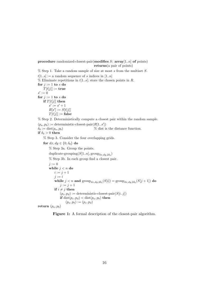
procedure randomized-closest-pair(modifies S: array[1..n] of points)returns(a pair of points)

% Step 1. Take a random sample of size at most s from the multiset S.

t[1..s] := a random sequence of s indices in [1..n]% Eliminate repetitions in t[1..s]; store the chosen points in R.for j := 1 to s do

T [t[j]] := true

s′ := 0for j := 1 to s do

if T [t[j]] then

s′ := s′ + 1R[s′] := S[t[j]]T [t[j]] := false

% Step 2. Deterministically compute a closest pair within the random sample.

(pa, pb) := deterministic-closest-pair(R[1..s′])δ0 := dist(pa, pb) % dist is the distance function.if δ0 > 0 then

% Step 3. Consider the four overlapping grids.

for dx, dy ∈ 0, δ0 do

% Step 3a. Group the points.

duplicate-grouping(S[1..n], groupdx,dy,2δ0)

% Step 3b. In each group find a closest pair.

j := 0while j < n do

i := j + 1j := iwhile j < n and groupdx,dy,2δ0

(S[i]) = groupdx,dy,2δ0(S[j + 1]) do

j := j + 1if i 6= j then

(pc, pd) := deterministic-closest-pair(S[i..j])if dist(pc, pd) < dist(pa, pb) then

(pa, pb) := (pc, pd)return (pa, pb)

Figure 1: A formal description of the closest-pair algorithm.

16

Remark 3.2 The randomized closest-pair algorithm generalizes naturally to anyd-dimensional space. Note that while two shifts (by 0 and δ0) of 2δ0-grids areneeded in the one-dimensional case, in the two-dimensional case 4 and in thed-dimensional case 2d shifted grids must be taken into account.

Remark 3.3 For implementing the procedure “deterministic-closest-pair” any ofa number of algorithms can be used. Small input sets are best handled by the“brute-force” algorithm, which calculates the distances between all n(n−1)/2 pairsof points; in particular, all calls to “deterministic-closest-pair” in Step 3b are exe-cuted in this way. For larger input sets, in particular, for the call to “deterministic-closest-pair” in Step 2, we use an asymptotically faster algorithm. For differentnumbers d of dimensions various algorithms are available. In the one-dimension-al case the closest-pair problem can be solved by sorting the points and findingthe minimum distance between two consecutive points. In the two-dimensionalcase one can use the simple plane-sweep algorithm of Hinrichs et al. [17]. In themulti-dimensional case, the divide-and-conquer algorithm of Bentley and Shamos[7] and the incremental algorithm of Schwarz et al. [30] are applicable. Assumingd to be constant, all the algorithms mentioned above run in O(n logn) time andO(n) space. One should be aware, however, that the complexity depends heavilyon d.

4 Analysis of the closest-pair algorithm

In this section, we prove that the algorithm given in Section 3 has linear timecomplexity with high probability. Again, we treat only the two-dimensional casein detail. Time bounds for most parts of the algorithm were established in previoussections or are immediately clear: Step 1 of the algorithm (taking the sample ofsize s′ ≤ s) obviously uses O(s) time. Since we assumed that s = O(n/ logn), nomore than O(n) time is consumed in Step 2 for finding a closest pair within thesample (see Remark 3.3). The complexity of the grouping performed in Step 3awas analyzed in Section 2. In order to implement the function groupdx,dy,δ, whichreturns the group indices, we need some preprocessing that takes O(n) time.

It remains only to analyze the cost of Step 3b, where closest pairs are foundwithin each group. It will be shown that a sample of size s ≥ 18n1/2+c, for any fixedc with 0 < c < 1/2, guarantees O(n)-time performance with a failure probabilityof at most 2−nc

. This holds even if a closest pair within each group is computed bythe brute-force algorithm (see Remark 3.3). On the other hand, if the samplingprocedure is modified in such a way that only a few 4-wise independent sequencesare used to generate the sampling indices t1, . . . , ts, linear running time will stillbe guaranteed with probability 1−O(n−α), for some constant α, while the numberof random bits needed is drastically reduced.

The analysis is complicated by the fact that points may occur repeatedly inthe multiset S = p1, . . . , pn. Of course, the algorithm will return two identicalpoints pa and pb in this case, and the minimum distance is 0. Note that in

17

Rabin’s paper [27] as well as in that of Khuller and Matias [19], the input pointsare assumed to be distinct.

Adapting a notion from [27], we first define what it means that there are“many” duplicates and show that in this case the algorithm runs fast. The longerpart of the analysis then deals with the situation where there are few or no du-plicate points. For reasons of convenience we will assume throughout the analysisthat n ≥ 800.

For a finite (multi)set S and a partition D = (S1, . . . , Sm) of S into nonemptysubsets, let

N(D) =m∑

µ=1

1

2|Sµ| · (|Sµ| − 1),

which is the number of (unordered) pairs of elements of S that lie in the sameset Sµ of the partition. In the case of the natural partition DS of the multisetS = p1, . . . , pn, where each class consists of all copies of one of the points, weuse the following abbreviation:

N(S) = N(DS) = |i, j | 1 ≤ i < j ≤ n and pi = pj|.

We first consider the case where N(S) is large; more precisely, we assume forthe time being that N(S) ≥ n. In Section B of the appendix it is proved thatunder this assumption, if we pick a sample of somewhat more than

√n random

elements of S, with high probability the sample will contain at least two equalpoints. More precisely, Corollary B.2 shows that the s ≥ 18n1/2+c sample pointschosen in Step 1 of the algorithm will contain two equal points with probabilityat least 1 − 2−nc

. The deterministic closest-pair algorithm invoked in Step 2 willidentify one such pair of duplicates and return δ0 = 0; at this point the algorithmterminates, having used only linear time.

For the remainder of this section we assume that there are not too manyduplicate points, that is, that N(S) < n. In this case, we may follow the argumentfrom Rabin’s paper. If G is a grid in the plane, then G induces a partition DS,G

of the multiset S into disjoint subsets S1, . . . , Sm (with duplicates)—two points ofS are in the same subset of the partition if and only if they fall into the same cellof G. As in the special case of N(S) above, we are interested in the number

N(S, G) = N(DS,G) = |i, j | pi and pj lie in the same cell of the grid G|.

This notion, which was also used in Rabin’s analysis [27], expresses the work donein Step 3b when the subproblems are solved by the brute-force algorithm.

Lemma 4.1 [27] Let S be a multiset of n points in the plane. Further, let G bea grid with resolution δ, and let G′ be one of the four grids with resolution 2δ thatoverlap G. Then N(S, G′) ≤ 4N(S, G) + 3

2n.

Proof. We consider 4 cells of G whose union is one cell of G′. Assume that these 4cells contain k1, k2, k3, and k4 points from S (with duplicates), respectively. The

18

contribution of these cells to N(S, G) is b = 12

∑4i=1 ki(ki − 1). The contribution

of the one (larger) cell to N(S, G′) is 12k(k − 1), where k =

∑4i=1 ki. We want to

give an upper bound on 12k(k − 1) in terms of b.

The function x 7→ x(x − 1) is convex in [0,∞). Hence

14k(

14k − 1

)

≤ 14

∑4i=1 ki(ki − 1) = 1

2b.

This implies

12k(k − 1) = 1

2k(k − 4) + 3

2k ≤ 8 · 1

4k(

14k − 1

)

+ 32k ≤ 4 · b + 3

2k.

Summing the last inequality over all cells of G′ yields the desired inequalityN(S, G′) ≤ 4N(S, G) + 3

2n.

Remark 4.2 In the case of d-dimensional space, this calculation can be carriedout in exactly the same way; this results in the estimate N(S, G′) ≤ 2dN(S, G) +12(2d − 1)n.

Corollary 4.3 Let S be a multiset of n points that satisfies N(S) < n. Thenthere is a grid G∗ with n ≤ N(S, G∗) < 5.5n.

Proof. We start with a grid G so fine that no cell of the grid contains two distinctpoints in S. Then, obviously, N(S, G) = N(S) < n. By repeatedly doubling thegrid size as in Lemma 4.1 until N(S, G′) ≥ n for the first time, we find a grid G∗

satisfying the claim.

Corollary 4.4 Let S be a multiset of size n and let G be a grid with resolution δ.Further, let G′ be an arbitrary grid with resolution at most δ. Then N(S, G′) ≤16N(S, G) + 6n.

Proof. Let Gi, for i = 1, 2, 3, 4, be the four different grids with resolution 2δ thatoverlap G. Each cell of G′ is completely contained in some cell of at least one ofthe grids Gi. Thus, the sets of the partition induced by G′ can be divided into fourdisjoint classes depending on which of the grids Gi covers the corresponding cellcompletely. Therefore, we have N(S, G′) ≤ ∑4

i=1 N(S, Gi). Applying Lemma 4.1and summing up yields N(S, G′) ≤ 16N(S, G) + 6n, as desired.

Now we are ready for analyzing Step 3b of the algorithm. As stated above, weassume that N(S) < n; hence the existence of some grid G∗ as in Corollary 4.3 isensured. Let δ∗ > 0 denote the resolution of G∗.

We apply Corollary B.2 from the appendix to the partition of S (with du-plicates) induced by G∗ to conclude that with probability at least 1 − 2−nc

therandom sample taken in Step 1 of the algorithm contains two points from thesame cell of G∗. It remains to show that if this is the case then Step 3b of thealgorithm takes O(n) time.

Since the real number δ0 calculated by the algorithm in Step 2 is bounded bythe distance of two points in the same cell of G∗, we must have δ0 ≤ 2δ∗. (This

19

is the case even if in Step 2 the Manhattan metric L1 is used.) Thus the fourgrids G1, G2, G3, G4 used in Step 3 have resolution 2δ0 ≤ 4δ∗. We form a newconceptual grid G∗∗ with resolution 4δ∗ by omitting all but every fourth line fromG∗. By the inequality N(S, G∗) < 5.5n (Corollary 4.3) and a double application ofLemma 4.1, we obtain N(S, G∗∗) = O(n). The resolution 4δ∗ of the grid G∗∗ is atleast 2δ0. Hence we may apply Corollary 4.4 to obtain that the four grids G1, G2,G3, G4 used in Step 3 of the algorithm satisfy N(S, Gi) = O(n), for i = 1, 2, 3, 4.But obviously the running time of Step 3b is O(

∑4i=1(N(S, Gi)+n)); by the above,

this bound is linear in n. This finishes the analysis of the cost of Step 3b.It is easy to see that Corollaries 4.3 and 4.4 as well as the analysis of Step 3b

generalize from the plane to any fixed dimension d. Combining the discussionabove with Theorem 2.13, we obtain the following.

Theorem 4.5 The closest-pair problem for a multiset of n points in d-dimension-al space, where d ≥ 1 is a fixed integer, can be solved by a randomized algorithmthat needs O(n) space and

(1) O(n) time on a real RAM with operations from +,−, ∗,div, log2, exp2;or

(2) O(n+log log(δmax/δmin)) time on a real RAM with operations from +,−, ∗,div,

where δmax and δmin denote the maximum and the minimum distance between anytwo distinct points, respectively. The probability that the time bound is exceeded is2−nΩ(1)

.

Proof. The running time of the randomized closest-pair algorithm is dominatedby that of Step 3a. The group indices used in Step 3a are d-tuples of integersin the range 0, . . . , ⌈δmax/δmin⌉. By Theorem 2.14, parts (1) and (2) of thetheorem follow directly from the corresponding parts of Theorem 2.13. Since allthe subroutines used finish within their respective time bounds with probability1−2−nΩ(1)

, the same is true for the whole algorithm. The amount of space requiredis obviously linear.

In the situation of Theorem 4.5, if the coordinates of the input points happento be integers drawn from a range 0, . . . , U −1, we can replace the real RAM bya conservative unit-cost RAM with integer operations; the time bound of part (2)then becomes O(n+log log U). The number of random bits used by either versionof the algorithm is quite large, namely essentially as large as possible with thegiven running time. Even if the number of random bits used is severely restricted,we can still retain an algorithm that is polynomially reliable.

Theorem 4.6 Let α, d ≥ 1 be arbitrary fixed integers. The closest-pair problemfor a multiset of n points in d-dimensional space can be solved by a randomizedalgorithm with the time and space requirements stated in Theorem 4.5 that usesonly O(log n + log(δmax/δmin)) random bits (or O(log n + log U) random bits forinteger input coordinates in the range 0, . . . , U − 1), and that exceeds the timebound with probability O(n−α).

20

Proof. We let s = 16α · ⌈n3/4⌉ and generate the sequence t1, . . . , ts in the algo-rithm as the concatenation of 4α independently chosen sequences of 4-independentrandom values that are approximately uniformly distributed in 1, . . . , n. Thisrandom experiment and its properties are described in detail in Corollary B.4 andLemma B.5 in Section B of the appendix. The time needed is o(n), and the num-ber of random bits needed is O(log n). The duplicate grouping is performed withthe simple method described in Section 2.3. This requires only O(log(δmax/δmin))or O(log U) random bits. The analysis is exactly the same as in the proof ofTheorem 4.5, except that Corollary B.4 is used instead of Corollary B.2.

5 Conclusions

We have provided an asymptotically efficient algorithm for computing a closestpair of n points in d-dimensional space. The main idea of the algorithm is touse random sampling in order to reduce the original problem to a collection ofduplicate-grouping problems. The performance of the algorithm depends on theoperations assumed to be primitive in the underlying machine model. We provedthat, with high probability, the running time is O(n) on a real RAM capable ofexecuting the arithmetic operations from +,−, ∗,div, log2, exp2 in constanttime. Without the operations log2 and exp2, the running time increases by anadditive term of O(log log(δmax/δmin)), where δmax and δmin denote the maximumand the minimum distance between two distinct points, respectively. When thecoordinates of the points are integers in the range 0, . . . , U − 1, the runningtimes are O(n) and O(n + log log U), respectively. For integer data the algorithmis conservative, i.e., all the numbers manipulated contain O(log n + log U) bits.

We proved that the bounds on the running times hold also when the collectionof input points contains duplicates. As an immediate corollary of this result weget that the following decision problems, which are often used in lower-boundarguments for geometric problems (see [26]), can be solved as efficiently as theone-dimensional closest-pair problem on the real RAM (Theorems 4.5 and 4.6):

(1) Element-distinctness problem: Given n real numbers, decide if any two ofthem are equal.

(2) ε-closeness problem: Given n real numbers and a threshold value ε > 0,decide if any two of the numbers are at distance less than ε from each other.

Finally, we would like to mention practical experiments with our simple dup-licate-grouping algorithm. The experiments were conducted by Tomi Pasanen(University of Turku, Finland). He found that the duplicate-grouping algorithmdescribed in Theorem 2.7, which is based on radix sort (with α = 3), behaves es-sentially as well as heapsort. For small inputs (n < 50 000) heapsort was slightlyfaster, whereas for large inputs heapsort was slightly slower. Randomized quick-sort turned out to be much faster than any of these algorithms for all n ≤ 1 000 000.One drawback of the radix-sort algorithm is that it requires extra memory space

21

for linking the duplicates, whereas heapsort (as well as in-place quicksort) does notrequire any extra space. One should also note that in some applications the wordlength of the actual machine can be restricted to, say, 32 bits. This means thatwhen n > 211 and α = 3, the hash function h ∈ Hk,ℓ (see the proof of Theorem2.7) is not needed for collapsing the universe; radix sort can be applied directly.Therefore the integers must be long before the full power of our methods comesinto play.

Acknowledgements

We would like to thank Ivan Damgard for his comments concerning Lemma A.1and Tomi Pasanen for his assistance in evaluating the practical efficiency of theduplicate-grouping algorithm. The question of whether the class of multiplicativehash functions is universal was posed to the first author by Ferri Abolhassan andJorg Keller. We also thank Kurt Mehlhorn for useful comments on this universalclass and on the issue of 4-independent sampling.

References

[1] A. Aggarwal, H. Edelsbrunner, P. Raghavan, and P. Tiwari, Op-timal time bounds for some proximity problems in the plane, Inform. Process.Lett. 42 (1992), 55–60.

[2] A.V. Aho, J. E. Hopcroft, and J. D. Ullman, “The Design and Anal-ysis of Computer Algorithms”, Addison-Wesley, Reading, 1974.

[3] A. Andersson, T. Hagerup, S. Nilsson, and R. Raman, Sorting inlinear time?, in “Proc. 27th Annual ACM Symposium on the Theory ofComputing”, pp. 427–436, Association for Computing Machinery, New York,1995.

[4] H. Bast and T. Hagerup, Fast and reliable parallel hashing, in “Proc.3rd Annual ACM Symposium on Parallel Algorithms and Architectures”, pp.50–61, Association for Computing Machinery, New York, 1991.

[5] P. Beauchemin, G. Brassard, C. Crepeau, C. Goutier, and

C. Pomerance, The generation of random numbers that are probablyprime, J. Cryptology 1 (1988), 53–64.

[6] M. Ben-Or, Lower bounds for algebraic computation trees, in “Proc. 15thAnnual ACM Symposium on Theory of Computing”, pp. 80–86, Associationfor Computing Machinery, New York, 1983.

[7] J. L. Bentley and M. I. Shamos, Divide-and-conquer in multidimensionalspace, in “Proc. 8th Annual ACM Symposium on Theory of Computing”, pp.220–230, Association for Computing Machinery, New York, 1976.

22

[8] J. L. Carter and M.N. Wegman, Universal classes of hash functions,J. Comput. System Sci. 18 (1979), 143–154.

[9] B. Chor and O. Goldreich, On the power of two-point based sampling,J. Complexity 5 (1989), 96–106.

[10] T.H. Cormen, C. E. Leiserson, and R. L. Rivest, “Introduction toAlgorithms”, The MIT Press, Cambridge, 1990.

[11] I. Damgard, P. Landrock, and C. Pomerance, Average case errorestimates for the strong probable prime test, Math. Comp. 61 (1993), 177–194.

[12] M. Dietzfelbinger, A. Karlin, K. Mehlhorn, F. Meyer auf der

Heide, H. Rohnert, and R.E. Tarjan, Dynamic perfect hashing: Upperand lower bounds, SIAM J. Comput. 23 (1994), 738–761.

[13] M. Dietzfelbinger and F.Meyer auf der Heide, Dynamic hashingin real time, in “Informatik · Festschrift zum 60. Geburtstag von GunterHotz” (J. Buchmann, H. Ganzinger, and W. J. Paul, Eds.), Teubner-Textezur Informatik, Band 1, pp. 95–119, B.G. Teubner, Stuttgart, 1992.

[14] M.L. Fredman, J. Komlos and E. Szemeredi, Storing a sparse tablewith O(1) worst case access time, J. Assoc. Comput. Mach. 31 (1984), 538–544.

[15] S. Fortune and J. Hopcroft, A note on Rabin’s nearest-neighbor algo-rithm, Inform. Process. Lett. 8 (1979), 20–23.

[16] M. Golin, R. Raman, C. Schwarz, and M. Smid, Simple randomizedalgorithms for closest pair problems, Nordic J. Comput. 2 (1995), 3–27.

[17] K. Hinrichs, J. Nievergelt, and P. Schorn, Plane-sweep solves theclosest pair problem elegantly, Inform. Process. Lett. 26 (1988), 255–261.

[18] J. Katajainen and M. Lykke, “Experiments with universal hashing”,Technical Report 96/8, Dept. of Computer Science, Univ. of Copenhagen,Copenhagen, 1996.

[19] S. Khuller and Y. Matias, A simple randomized sieve algorithm for theclosest-pair problem, Inform. and Comput. 118 (1995), 34–37.

[20] D. Kirkpatrick and S. Reisch, Upper bounds for sorting integers onrandom access machines, Theoret. Comput. Sci. 28 (1984), 263–276.

[21] D.E. Knuth, “The Art of Computer Programming, Vol. 3: Sorting andSearching”, Addison-Wesley, Reading, 1973.

23

[22] Y. Mansour, N. Nisan, and P. Tiwari, The computational complexityof universal hashing, in “Proc. 22nd Annual ACM Symposium on Theory ofComputing”, pp. 235–243, Association for Computing Machinery, New York,1990.

[23] Y. Matias and U. Vishkin, “On parallel hashing and integer sorting”,Technical Report UMIACS–TR–90–13.1, Inst. for Advanced Computer Stud-ies, Univ. of Maryland, College Park, 1990. (Journal version: J. Algorithms12 (1991), 573–606.)

[24] K. Mehlhorn, “Data Structures and Algorithms, Vol. 1: Sorting andSearching”, Springer-Verlag, Berlin, 1984.

[25] G.L. Miller, Riemann’s hypothesis and tests for primality, J. Comput.System Sci. 13 (1976), 300–317.

[26] F.P. Preparata and M. I. Shamos, “Computational Geometry: An In-troduction”, Springer-Verlag, New York, 1985.

[27] M.O. Rabin, Probabilistic algorithms, in “Algorithms and Complexity:New Directions and Recent Results” (J. F. Traub, Ed.), pp. 21–39, AcademicPress, New York, 1976.

[28] M.O. Rabin, Probabilistic algorithm for testing primality, J. Number The-ory 12 (1980), 128–138.

[29] R. Raman, Priority queues: small, monotone and trans-dichotomous, in“Proc. 4th Annual European Symposium on Algorithms”, Lecture Notes inComput. Sci. 1136, pp. 121–137, Springer, Berlin, 1996.

[30] C. Schwarz, M. Smid, and J. Snoeyink, An optimal algorithm for theon-line closest-pair problem, in “Proc. 8th Annual Symposium on Computa-tional Geometry”, pp. 330–336, Association for Computing Machinery, NewYork, 1992.

[31] W. Sierpinski, “Elementary Theory of Numbers”, Second English Edition(A. Schinzel, Ed.), North-Holland, Amsterdam, 1988.

[32] A.C.-C. Yao, Lower bounds for algebraic computation trees with integerinputs, SIAM J. Comput. 20 (1991), 655–668.

A Generating primes

In this section we provide a proof of Lemma 2.9. The main idea is expressed inthe proof of the following lemma.

24

Lemma A.1 There is a randomized algorithm that, for any given integer m ≥ 2,returns an integer p with m < p ≤ 2m such that the following holds: the runningtime is O((log m)4), and the probability that p is not prime is at most 1/m.

Proof. The heart of the construction is the randomized primality test due to Miller[25] and Rabin [28] (for a description and an analysis see, e. g., [10, pp. 839 ff.]). Ifan arbitrary number x of b bits is given to the test as an input, then the followingholds:

(a) If x is prime, then Prob(the result of the test is “prime”) = 1;

(b) if x is composite, then Prob(the result of the test is “prime”) ≤ 1/4;

(c) performing the test once requires O(b) time, and all numbers manipulatedin the test are O(b) bits long.

By repeating the test t times, the reliability of the result can be increased suchthat for composite x we have

Prob(the result of the test is “prime”) ≤ 1/4t.

In order to generate a “probable prime” that is greater than m we use a randomsampling algorithm. We select s (to be specified later) integers from the intervalm + 1, . . . , 2m at random. Then these numbers are tested one by one until theresult of the test is “prime”. If no such result is obtained the number m + 1 isreturned.

The algorithm fails to return a prime number (1) if there is no prime amongthe numbers in the sample, or (2) if one of the composite numbers in the sampleis accepted by the primality test. We estimate the probabilities of these events.

It is known that the function π(x) = |p| p ≤ x and p is prime|, defined forany real number x, satisfies

π(2n) − π(n) >n

3 ln(2n),

for all integers n > 1. (For a complete proof of this fact, also known as theinequality of Finsler, see [31, Sections 3.10 and 3.14].) That is, the number ofprimes in the set m + 1, . . . , 2m is at least m/(3 ln(2m)). We choose

s = s(m) = ⌈3(ln(2m))2⌉

andt = t(m) = max⌈log2s(m)⌉ , ⌈log2(2m)⌉.

(Note that t(m) = O(log m).) Then the probability that the random samplecontains no prime at all is bounded by

(

1 − 1

3 ln(2m)

)s

≤

(

1 − 1

3 ln(2m)

)3 ln(2m)

ln(2m)

< e− ln(2m) =1

2m.

25

The probability that one of the at most s composite numbers in the sample willbe accepted is smaller than

s(m) · (1/4)t ≤ s(m) · 2− log2s(m) · 2− log2(2m) =1

2m.

Summing up, the failure probability of the algorithm is at most 2 · (1/(2m)) =1/m, as claimed. If m is a b-bit number, the time required is O(s · t · b), that is,O((log m)4).

Remark A.2 The problem of generating primes is discussed in greater detail byDamgard et al. [11]. Their analysis shows that the proof of Lemma A.1 is overlypessimistic. Therefore, without sacrificing the reliability, the sample size s and/orthe repetition count t can be decreased; in this way considerable savings in therunning time are possible.

Lemma 2.9 There is a randomized algorithm that, for any given positive integersm and n with 2 ≤ m ≤ 2⌈n

1/4⌉, returns a number p with m < p ≤ 2m such thatthe following holds: the running time is O(n), and the probability that p is not

prime is at most 2−n1/4.

Proof. We increase the sample size s and the repetition count t in the algorithmof Lemma A.1 above, as follows:

s = s(m, n) = 6 · ⌈ln(2m)⌉ · ⌈n1/4⌉

andt = t(m, n) = 1 + max⌈log2s(m, n)⌉, ⌈n1/4⌉.

As above, the failure probability is bounded by the sum of the following two terms:

(

1 − 1

3 ln(2m)

)s(m,n)

< e−2⌈n1/4⌉ < 2−1−n1/4

ands(m, n) · (1/4)t(m,n) ≤ 2−(1+⌈n1/4⌉) ≤ 2−1−n1/4

.

This proves the bound 2−n1/4on the failure probability. The running time is

O(s · t · log m) = O((log m) · n1/4 · (log log m + log n + n1/4) · log m) = O(n).

26

B Random sampling in partitions

In this section we deal with some technical details of the analysis of the closest-pair algorithm. For a finite set S and a partition D = (S1, . . . , Sm) of S intononempty subsets, let

P (D) = π ⊆ S | |π| = 2 ∧ ∃µ ∈ 1, . . . , m : π ⊆ Sµ.

Note that the quantity N(D) defined in Section 4 equals |P (D)|. For the analysisof the closest-pair algorithm, we need the following technical fact: If N(D) islinear in n and more than 8

√n elements are chosen at random from S, then with a

probability that is not too small two elements from the same subset of the partitionare picked. A similar lemma was proved by Rabin [27, Lemma 6]. In Section B.1we give a totally different proof, resting on basic facts from probability theory (viz.,Chebyshev’s inequality), which may make it more conspicuous why the lemma istrue than Rabin’s proof. Further, it will turn out that full independence of theelements in the random sample is not needed, but rather that 4-wise independenceis sufficient. This observation is crucial for a version of the closest-pair algorithmthat uses only few random bits. The technical details are given in Section B.2.

B.1 The sampling lemma

Lemma B.1 Let n, m and s be positive integers, let S be a set of size n ≥ 800,let D = (S1, . . . , Sm) be a partition of S into nonempty subsets with N(D) ≥ n,and assume that s random elements t1, . . . , ts are drawn independently from theuniform distribution over S. Then if s ≥ 8

√n,

Prob(

∃i, j ∈ 1, . . . , s∃µ ∈ 1, . . . , m : ti 6= tj ∧ ti, tj ∈ Sµ

)

> 1− 4√

n

s. (B.1)

Proof. We first note that we may assume, without loss of generality, that

n ≤ N(D) ≤ 1.1n. (B.2)

To see this, assume that N(D) > 1.1n and consider a process of repeatedly refiningD by splitting off an element x in a largest set in D, i.e., by making x into asingleton set. As long as D contains a set of size

√2n + 2 or more, the resulting

partition D′ still has N(D′) ≥ n. On the other hand, splitting off an element from

a set of size less that√

2n+2 changes N by less than√

2n+1 =√

200/n ·0.1n+1,which for n ≥ 800 is at most 0.1n. Hence if we stop the process with the firstpartition D′ with N(D′) ≤ 1.1n, we will still have N(D′) ≥ n. Since D′ is arefinement of D, we have for all i and j that

ti and tj are contained in the same set S ′µ of D′

⇒ ti and tj are contained in the same set Sµ of D;

thus, it suffices to prove (B.1) for D′.

27

We define random variables Xπi,j, for π ∈ P (D) and 1 ≤ i < j ≤ s, as follows:

Xπi,j :=

1 if ti, tj = π,0 otherwise.

Further, we letX =

∑

π∈P (D)

∑

1≤i<j≤s

Xπi,j.

Clearly, by the definition of P (D),

X = |(i, j) | 1 ≤ i < j ≤ s ∧ ti 6= tj ∧ ti, tj ∈ Sµ for some µ | ≥ 0.

Thus, to establish (B.1), we only have to show that

Prob(X = 0) <4√

n

s.

For this, we estimate the expectation E(X) and the variance Var(X) of therandom variable X, with the intention of applying Chebyshev’s inequality:

Prob(

|X −E(X)| ≥ t)

≤ Var(X)

t2, for all t > 0. (B.3)

(For another, though simpler, application of Chebyshev’s inequality in a similarcontext see [9]).

First note that for each π = x, y ∈ P (D) and 1 ≤ i < j ≤ s the followingholds:

E(Xπi,j) = Prob(ti = x ∧ tj = y) + Prob(ti = y ∧ tj = x) =

2

n2. (B.4)

Thus,

E(X) =∑

π∈P (D)

∑

1≤i<j≤s

E(Xπi,j) (B.5)

= |P (D)| ·(

s

2

)

· 2

n2= N(D) · s2

n2·(

1 − 1

s

)

.

By assumption, s ≥ 8√

n ≥ 8√

800, so that 1 − 1/s ≥ 1/1.01. Let α = s/√

n.Using the assumption N(D) ≥ n, we get from (B.5) that

E(X) ≥ α2

1.01. (B.6)

Next we derive an upper bound on the variance of X. With the (standard)notation

Cov(Xπi,j, X

π′

i′,j′) = E(Xπi,j · Xπ′

i′,j′) − E(Xπi,j) · E(Xπ′

i′,j′)

28

we may write

Var(X) = E(X2) − (E(X))2 =∑

π,π′∈P (D)

∑

1≤i<j≤s1≤i′<j′≤s

Cov(Xπi,j, X

π′

i′,j′). (B.7)

We split the summands Cov(Xπi,j, X

π′

i′,j′) occurring in this sum into several classesand estimate the contribution to Var(X) of the summands in each of these classes.For all except the first class, we use the simple bound

Cov(Xπi,j, X

π′

i′,j′) ≤ E(Xπi,j · Xπ′

i′,j′) = Prob(Xπi,j = Xπ′

i′,j′ = 1).

For i ∈ 1, . . . , s, if ti = x ∈ S, we will say that i is mapped to x. Below webound the probability that i, j is mapped onto π, while at the same time i′, j′is mapped onto π′. Let J = i, j, i′, j′.

Class 1. |J | = 4. In this case the random variables Xπi,j and Xπ′

i′,j′ are inde-

pendent, so that Cov(Xπi,j, X

π′

i′,j′) = 0.

Class 2. |J | = 2 and π = π′. Now E(Xπi,j · Xπ′

i′,j′) = E(Xπi,j), so the total

contribution to Var(X) of summands of Class 2 is at most

∑

π∈P (D)

∑

1≤i<j≤s

E(Xπi,j) = E(X).

Class 3. |J | < |π ∪ π′|. In this case J cannot be mapped onto π ∪ π′, soXπ

i,j · Xπ′

i′,j′ ≡ 0 and Cov(Xπi,j, X

π′

i′,j′) ≤ 0.Since |J | ∈ 2, 3, 4 and |π ∪ π′| ∈ 2, 3, 4, the only case not covered above

is |J | = 3 and |π ∪ π′| ∈ 2, 3. In order to simplify the discussion of this finalcase, let us call the single element of i, j ∩ i′, j′ the central domain element.Correspondingly, if |π ∪ π′| = 3, we call the single element of π ∩ π′ the centralrange element. The argument proceeds by counting the number of summands ofcertain kinds as well as estimating the size of each summand.

Class 4. |J | = 3 and |π ∪ π′| ∈ 2, 3. The central domain element and theother elements of i, j and i′, j′ can obviously be chosen in no more than s3

ways.Class 4a. |J | = 3 and π = π′. By definition, π = π′ can be chosen in

N(D) ways. Furthermore, Xπi,j = Xπ

i′,j′ = 1 only if the central domain elementis mapped to one element of π, while the two remaining elements of J are bothmapped to the other element of π, the probability of which is (2/n)(1/n)(1/n) =2/n3. Altogether, the contribution to Var(X) of summands of Class 4a is at mosts3 · N(D) · 2/n3 ≤ 2.2s3/n2.

Class 4b. |J | = 3 and |π∪π′| = 3. The set π∪π′ can be chosen in∑m

µ=1

(

|Sµ|3

)

ways, after which there are three choices for the central range element and twoways of completing π (and, implicitly, π′) with one of the remaining elements ofπ ∪ π′. Xπ

i,j = Xπ′

i′,j′ = 1 only if the central domain element is mapped to thecentral range element, while the remaining element of i, j is mapped to theremaining element of π and the remaining element of i′, j′ is mapped to the

29

remaining element of π′, the probability of which is 1/n3. It follows that the totalcontribution to Var(X) of summands of Class 4b is bounded by

m∑

µ=1

|Sµ|(|Sµ| − 1)(|Sµ| − 2)

·(

s

n

)3

≤

m∑

µ=1

(|Sµ| − 1)3

·(

s

n

)3

. (B.8)

We use the inequality∑m

µ=1 a3µ ≤

(

∑mµ=1 a2

µ

)3/2(a special case of Jensen’s inequal-

ity, valid for all a1, . . . , am ≥ 0) and the assumption (B.2) to bound the right handside in (B.8) by

m∑

µ=1

|Sµ|(|Sµ| − 1)

3/2

·(

s

n

)3

≤ (2 · 1.1n)3/2 ·(

s

n

)3

= 2.23/2 ·(

s√n

)3

< 3.3α3.

Bounding the contributions of the summands of the various classes to the sum inequation (B.7), we get (using that n1/2 ≥ 25)

Var(X) ≤ E(X) + 2.2s3/n2 + 3.3α3 = E(X) + (2.2n−1/2 + 3.3)α3

< E(X) + 3.5α3. (B.9)

By (B.3) we have

Prob(X = 0) ≤ Prob(

|X − E(X)| ≥ E(X))

≤ Var(X)

(E(X))2;

by (B.9) and (B.6) this yields

Prob(X = 0) ≤ 1

E(X)+

3.5α3

(E(X))2≤ 1.01

α2+

3.5 · 1.012

α.

Since 1.01/α + 3.5 · 1.012 < 4, we get

Prob(X = 0) <4

α=

4√

n

s,

as claimed.

In case the size of the chosen subset is much larger than√

n, the estimate inthe lemma can be considerably sharpened.

Corollary B.2 Let n, m and s be positive integers, let S be a set of size n ≥ 800,let D = (S1, . . . , Sm) be a partition of S into nonempty subsets with N(D) ≥ n,and assume that s random elements t1, . . . , ts are drawn independently from theuniform distribution over S. Then if s ≥ 9

√n,

Prob(

∃i, j ∈ 1, . . . , s∃µ ∈ 1, . . . , m : ti 6= tj ∧ ti, tj ∈ Sµ

)

> 1 − 2−s/(18√

n).

30

Proof. Split the sequence t1, . . . , ts into disjoint subsequences of length s′ = ⌈8√n⌉≤ 9

√n each, with fewer than s′ elements left over. By Lemma B.1, in each of

the corresponding subexperiments the probability that two elements in the samesubset Sµ are hit is at least 1 − 4

√n/s′ ≥ 1

2. Since the subexperiments are

independent and their number is at least ⌊s/(9√

n)⌋ ≥ s/(18√

n), the statedevent will occur in at least one of them with probability at least 1 − 2−s/(18

√n).

Clearly, this is also a lower bound on the probability that the whole sequencet1, . . . , ts hits two elements from the same Sµ.

B.2 Sampling with few random bits

In this section we show that the effect described in Lemma B.1 can be achievedalso with a random experiment that uses very few random bits.

Corollary B.3 Let n, m, s, S, and D be as in Lemma B.1. Then the conclusionof Lemma B.1 also holds if the s elements t1, . . . , ts are chosen according to adistribution over S that only satisfies the following two conditions:

(a) the sequence is 4-independent, i. e., for all sets i, j, k, ℓ ⊆ 1, . . . , s ofsize 4 the values ti, tj, tk, tℓ are independent; and

(b) for all i ∈ 1, . . . , s and all x ∈ S we have

1 − ε

n< Prob(ti = x) <

1 + ε

n,

where ε = 0.0025.

Proof. This is proved almost exactly as Lemma B.1. We indicate the slight changesthat have to be made. Equation (B.4) is replaced by

E(Xπi,j) ≥ 2 ·

(

1 − ε

n

)2

≥ 2(1 − 2ε)

n2.

Equation (B.5) changes into

E(X) ≥ N(D) · s2

n2· (1 − 2ε) ·

(

1 − 1

s

)

.

As s ≥ 8√

800 and ε = 0.0025, we get (1− 2ε)(1− 1/s) ≥ 1/1.01, such that (B.6)remains valid. The contributions to Var(X) of the summands of the variousclasses defined in the proof of Lemma B.1 are bounded as follows.

Class 1: The contribution is 0. For justifying this, 4-wise independence is suffi-cient.

Class 2: E(X).

Class 3: ≤ 0.

31

Class 4a: s3 · N(D) · (2/n3) · (1 + ε)3 ≤ 2.3s3/n2.

Class 4b: (2.2n)3/2 · (s/n3) · (1 + ε)3 ≤ 3.3α3.

Finally, estimate (B.9) is replaced by

Var(x) ≤ E(X) + (2.3n−1/2 + 3.3)α3 < E(X) + 3.5α3,

where we used that n1/2 ≥ 25. The rest of the argument is verbally the same asin the proof of Lemma B.1.

In the random sampling experiment, we can even achieve polynomial reliabilitywith a moderate number of random bits.

Corollary B.4 In the situation of Lemma B.1, let s ≥ 4⌈n3/4⌉, and let α ≥ 1be an arbitrary integer. If the experiment described in Corollary B.3 is repeatedindependently 4α times to generate 4α sequences (tℓ,1, . . . , tℓ,s), with 1 ≤ ℓ ≤ 4α,of elements of S, then

Prob(

∃k, ℓ ∈ 1, . . . , 4α∃i, j ∈ 1, . . . , s∃µ ∈ 1, . . . , m :

tk,i 6= tℓ,j ∧ tk,i, tℓ,j ∈ Sµ

)

> 1 − n−α.

Proof. By Corollary B.3, for each fixed ℓ the probability that the sequence tℓ,1, . . . ,tℓ,s hits two different elements in the same subset Sµ is at least 1 − 4

√n/s ≥

1 − n−1/4. By independence, the probability that this happens for one of the4α sequences is at least 1 − (n−1/4)4α; clearly, this is also a lower bound on theprobability that the whole sequence tℓ,i, with 1 ≤ ℓ ≤ 4α and 1 ≤ i ≤ s, hits twodifferent elements in the same set Sµ.

Lemma B.5 Let S = 1, . . . , n for some n ≥ 800 and take s = 4⌈n3/4⌉. Thenthe random experiment described in Corollary B.3 can be carried out in o(n) timeusing a sample space of size O(n6) (or, informally, using 6 log2n + O(1) randombits).

Proof. Let us assume for the time being that a prime number p with s < p ≤ 2s isgiven. (We will see at the end of the proof how such a p can be found within thetime bound claimed.) According to [9], a 4-independent sequence t′1, . . . , t

′p, where

each t′j is uniformly distributed in 0, . . . , p − 1, can be generated as follows:Choose 4 coefficients γ′

0, γ′1, γ

′2, γ

′3 randomly from 0, . . . , p − 1 and let

t′j =

(

3∑

r=0

γ′r · jr

)

mod p, for 1 ≤ j ≤ p.

By repeating this experiment once (independently), we obtain another such se-quence t′′1, . . . , t

′′p. We let

tj = 1 + (t′j + pt′′j ) mod n, for 1 ≤ j ≤ s.

32

Clearly, the overall size of the sample space is (p4)2 = p8 = O(n6), and the timeneeded for generating the sample is O(s). We must show that the distribution oft1, . . . , ts satisfies conditions (a) and (b) of Corollary B.3. Since the two sequences(t′p, . . . , t

′p) and (t′′p, . . . , t

′′p) originate from independent experiments and each of

them is 4-independent, the sequence

t′1 + pt′′1, . . . , t′s + pt′′s

is 4-independent; hence the same is true for t1, . . . , ts, and (a) is proved. Further,t′j + pt′′j is uniformly distributed in 0, . . . , p2 − 1, for 1 ≤ j ≤ s. From this, it iseasily seen that, for x ∈ S,

Prob(tj = x) ∈⌊

p2

n

⌋

· 1

p2,

⌈

p2

n

⌉

· 1

p2

.

Now observe that ⌊p2/n⌋ /p2 < 1/n < ⌈p2/n⌉ /p2, and that

⌈

p2

n

⌉

· 1

p2−⌊

p2

n

⌋

· 1

p2≤ 1

p2<

1

s2≤ 1

16n3/2=

1

16√

n· 1

n<

ε

n,

where we used that n ≥ 800, whence 1/(16√

n) < 1/400 = 0.0025 = ε. Thisproves (b).

Finally, we briefly recall the fact that a prime number in the range s +1, . . . , 2s can be found deterministically in time O(s log log s). (Note that weshould not use randomization here, as we must take care not to use too manyrandom bits.) The straightforward implementation of the Eratosthenes sieve (see,e. g., [31, Section 3.2]) for finding all the primes in 1, . . . , 2s has running time

O

(

s +∑

p≤√

2sp prime

⌈2s/p⌉)

= O

(

s ·(

1 +∑

p≤√

2sp prime

1

p

)

)

= O(s log log s),

where the last estimate results from the fact that

∑

p≤xp prime

1

p= O(log log x).

(For instance, this can easily be derived from the inequality π(2n) − π(n) <7n/(5 lnn), valid for all integers n > 1, which is proved in [31, Section 3.14].)

33