ArticleVolume 14, Number 6

19 June 2013

doi:10.1002/ggge.20129

ISSN: 1525-2027

A reference Earth model for the heat-producing elements andassociated geoneutrino flux

Yu HuangDepartment of Geology, University of Maryland, 237 Regents Drive, Geology Building, College Park,Maryland, 20742 USA (yuhuang@umd.edu)

Viacheslav ChubakovDipartimento di Fisica, Università degli Studi di Ferrara, Polo Scientifico e Tecnologico,Via Saragat 1 - I-44122, Ferrara, Italy

Istituto Nazionale di Fisica Nucleare, Sezione di Ferrara, Polo Scientifico e Tecnologico,Via Saragat 1 - I-44122, Ferrara, Italy

Fabio MantovaniDipartimento di Fisica, Università degli Studi di Ferrara, Polo Scientifico e Tecnologico,Via Saragat 1 - I-44122, Ferrara, Italy

Istituto Nazionale di Fisica Nucleare, Sezione di Ferrara, Polo Scientifico e Tecnologico,Via Saragat 1 - I-44122, Ferrara, Italy

Roberta L. RudnickDepartment of Geology, University of Maryland, 237 Regents Drive, Geology Building, College Park,Maryland, 20742 USA

William F. McDonoughDepartment of Geology, University of Maryland, 237 Regents Drive, Geology Building, College Park,Maryland, 20742 USA

[1] The recent geoneutrino experimental results from KamLAND (Kamioka Liquid Scintillator Anti-neutrino Detector) and Borexino detectors reveal the usefulness of analyzing the Earth’s geoneutrinoflux, as it provides a constraint on the strength of the radiogenic heat power, and this, in turn,provides a test of compositional models of the bulk silicate Earth (BSE). This flux is dependent on theamount and distribution of heat-producing elements (HPEs: U, Th, and K) in the Earth’s interior. We havedeveloped a geophysically based, three-dimensional global reference model for the abundances and distribu-tions of HPEs in the BSE. The structure and composition of the outermost portion of the Earth, the crust andunderlying lithospheric mantle, are detailed in the reference model; this portion of the Earth has the greatestinfluence on the geoneutrino fluxes. The reference model combines three existing geophysical models of theglobal crust and yields an average crustal thickness of 34.4� 4.1 km in the continents and 8.0� 2.7 km inthe oceans, and a total mass (in 1022 kg) of oceanic, continental, and bulk crust is 0.67� 0.23, 2.06� 0.25,and 2.73� 0.48, respectively. In situ seismic velocity provided by CRUST 2.0 allows us to estimate theaverage composition of the deep continental crust by using new and updated compositional databases foramphibolite and granulite facies rocks in combination with laboratory ultrasonic velocities measurements.An updated xenolithic peridotite database is used to represent the average composition of continentallithospheric mantle. Monte Carlo simulation is used to predict the geoneutrino flux at 16 selected locations

©2013. American Geophysical Union. All Rights Reserved. 2003

and to track the asymmetrical uncertainties of radiogenic heat power due to the log-normal distributions of HPEconcentrations in crustal rocks.

Components: 16,900 words, 8 tables, 10 figures.

Keywords: geoneutrino flux; heat producing element; radiogenic heat power; reference crustal model; deepcrust composition; bulk silicate Earth composition; Monte Carlo simulation.

Index Terms: 1020 Composition of the continental crust; 8130 Heat generation and transport; 1025 Compositionof the mantle; 1009 Geochemical modeling (3610, 8410); 1065 Major and trace element geochemistry.

Received 7 December 2012;Revised 18March 2013;Accepted 24March 2013;Published 19 June 2013.

Huang, Y., V. Chubakov, F. Mantovani, R. L. Rudnick, and W. F. McDonough (2013), A reference Earth model for the heat-producing elements and associated geoneutrino flux, Geochem. Geophys. Geosyst., 14, 2003–2029, doi:10.1002/ggge.20129.

1. Introduction

[2] Determining the Earth’s heat budget and heatproduction is critical for understanding plate tecton-ics and the thermal evolution of the Earth. Recentdetection of geoneutrinos (electron antineutrinosgenerated during beta decay) offers a means to deter-mine the U and Th concentrations in the Earth that iscomplementary to traditional cosmochemical or geo-chemical arguments [Dye, 2010]. However, since allthree existing geoneutrino detectors are currentlylocated within the continental crust (two in operation,another coming online in 2013), the crustal contribu-tion, which dominates the geoneutrino signal, mustbe subtracted in order to determine the signal fromthe mantle and core [Dye, 2012; Fiorentini et al.,2012; Šrámek et al., 2013].

[3] Here we develop a three-dimensional globalreference model that describes the inventory anddistribution of the heat-producing elements (HPEs:U, Th, and K) in the bulk silicate Earth (BSE),along with uncertainties. The greatest resolution ofthe model resides in the outermost portions of theEarth—the crust and underlying lithospheric man-tle—from whence the largest portion of the surfaceflux originates. The model is open-source and rep-resents the first step in an effort to develop commu-nity ownership.

1.1. Heat-producing Elements andEarth Differentiation

[4] Radioactivities of U, Th, and K contribute about99%, with a relative contribution of approximately2:2:1, of the total radiogenic heat power of theEarth. Although the heat production rate for unitmass of Rb at natural isotopic abundance is higherthan K, the contribution of Rb to the total

radiogenic heat power is expected to be less than1% [Fiorentini et al., 2007], given the relative de-cay rates, and a K/Rb ratio of ~400 in the BSE[McDonough and Sun, 1995]. The other elements,such as La and Sm, make negligible contributionsto the total radiogenic power.

[5] Uranium and Th are the refractory lithophileelements, while K is a volatile lithophile element.The lithophile classification means that HPEs areexpected to reside in the rocky portion of the Earth[Goldschmidt, 1933], though some have speculatedthat U and K may become slightly siderophile orchalcophile at high temperatures and pressuresand thus may enter the Earth’s core [e.g., Lewis,1971; Murrell and Burnett, 1986; Murthy et al.,2003]. The refractory nature of U and Th means thatthe Earth should have accreted with the full solar com-plement of these elements, whereas the volatility of Khas led to its depletion in the Earth relative to the Sunand primitive chondritic meteorites [e.g.,McDonough,2003]. Thus, the concentration of K in the Earth isinferred from analyses of geological samples and itsbehavior relative to refractory elements.

[6] Uranium, Th, and K are all highly incompatibleelements (defined as having crystal/melt partitioncoefficients much less than one) and, thus, are con-centrated in melts relative to residues during partialmelting. The Earth has experienced irreversibledifferentiation via melting and the ascent of thesemelts toward the surface, leading to the concentra-tion of these elements in the outermost layers ofthe planet. Thus, although the continental crustcomprises only ~0.5% of the mass of the BSE, itcontributes almost one third of the total radiogenicheat power, and refining the composition of thecontinental crust is an essential prerequisite tousing geoneutrinos to “see” into the deeper levelsof the Earth.

GeochemistryGeophysicsGeosystemsG3G3 HUANG ET AL.: EARTH MODEL HPE GEONEUTRINO 10.1002/ggge.20129

2004

[7] Compositional models for the BSE vary bynearly a factor of 3 in their U content (i.e., ~10 ng/g[Javoy et al., 2010; O’Neill and Palme, 2008],~20 ng/g [Allègre et al., 1995; Hart and Zindler,1986; Lyubetskaya and Korenaga, 2007a; 2007b;McDonough and Sun, 1995; Palme and O’Neill,2003], and ~30ng/g [Anderson, 2007; Turcotte andSchubert, 2002; Turcotte et al., 2001]). These modelsgenerally agree on a Th/U of 3.9 and a K/U of 14,000[Arevalo et al., 2009]. Compositional models for thecontinental crust (see summary in Rudnick and Gao[2003]) predict a U content of 1100 to 2700 ng/g,implying that anywhere between 30% and 45% ofthe budget of HPEs is stored in this thin skin of crustand that it is more than ~100-fold enriched over themodern mantle (i.e., ~13 ng/g of U), assuming a geo-chemical model for the BSE ofMcDonough and Sun[1995]. Geoneutrino data, when available for severalsites on the Earth, should be able to define permissi-ble models for the BSE and the continental crust.

1.2. Geoneutrinos

[8] The Earth is an electron antineutrino star thatemits these nearly massless particles at a rate of~106 cm�2 s�1 [e.g., Enomoto et al., 2007;Fiorentini et al., 2007; Kobayashi and Fukao,1991; Mantovani et al., 2004]. Geoneutrinos areelectron antineutrinos produced within the Earthby beta-minus decay when a neutron decays to aproton via the weak interaction. This decay process,in which a down quark transforms to an up quark, ismediated by the emission of a W� boson alongwith an electron, and a charge neutral electron anti-neutrino. Because of their vanishingly small crosssection for interaction, ~10�44 cm2, matter is virtu-ally transparent to these particles, and they haveabout a 50% chance of passing through a light-year of lead without interaction. By comparison,the fusion processes inside the core of the Sunproduce neutrinos, the antimatter lepton counterpartof antineutrinos, which bathe the Earth’s surface witha flux that is ~104 greater than the geoneutrino flux[Bahcall et al., 2005]. The term geoneutrino distin-guishes natural emissions of electron antineutrinosfrom those radiated from nuclear reactors.

[9] To date, geoneutrino flux measurements havebeen made at two detectors, Kamioka LiquidScintillator Antineutrino Detector (KamLAND), atthe Kamioka mine in Japan [Araki et al., 2005;Gando et al., 2011, 2013], and Borexino, at the GranSasso underground laboratories in Italy [Bellini et al.,2010, 2013], and provide constraints on the quanti-ties of U and Th inside the Earth. The Sudbury

Neutrino Observatory (SNO)+ detector at the Sud-bury Neutrino Observatory, Canada [Chen, 2006],will come online in 2014 and will deliver significantnew data on the geoneutrino flux from theArchean Superior Craton and surrounding NorthAmerican plate.

[10] Geoneutrinos originating from U and Th can bedistinguished based on their energy spectra, e.g.,geoneutrinos with E> 2.25MeV are produced onlyin the 238U chain [e.g., Araki et al., 2005]. Liquidscintillator detectors work by sensing light generatedduring antineutrino-proton interactions: �ve +p! e+ +n, when the �ve has ≥1.806MeV energy, which is theenergy needed to transform the proton, p, to a posi-tron e+ and a neutron, n. Of the total geoneutrinoflux, only small portions of antineutrinos generatedin the 238U and 232Th decay chains can be detectedby this mechanism. The hydrogen nuclei, whichare in abundant supply in hydrocarbon (CnH2n)-based liquid scintillator detectors, act as the targetfor transiting antineutrinos. The directionality ofantineutrinos is presently undetectable, and, thus,the detectors are sensitive only to the integrated flux.Fortunately, because the geoneutrino flux at a detec-tor decreases with distance from the source via theinverse square law, geoneutrinos can be used to de-tect regional differences in the distribution of U andTh in the continents and, in principle, large-scale fea-tures in the mantle [Dye, 2010; Šrámek et al., 2013].Thus, accurate and precise detection of the surfaceflux of geoneutrinos, coupled with geochemical andgeophysical models of local and global crust, willenable quantitative tests of compositional models ofthe planet.

1.3. Modeling the Earth’sHeat-producing Elements

[11] We can model the Earth’s geoneutrino flux byassigning physical and chemical data to a set ofspatially defined voxels (a volume element, compa-rable to a three-dimensional pixel). Such a modelcan be compared to surface heat flow measurementsand various mass balance models for the com-position of the Earth and its internal reservoirs(i.e., crust, mantle, and core). Toward this goal, anenormous amount of geophysical and geochemicaldata have been collected and shared online in the pastfew decades. This information can be integrated intoa broader framework in order to evaluate the natureand/or existence of planetary features, such as chem-ical compositions of thermochemical piles in themantle [Šrámek et al., 2013], the characteristics of aresidual layer from a basal magma ocean [Labrosse

GeochemistryGeophysicsGeosystemsG3G3 HUANG ET AL.: EARTH MODEL HPE GEONEUTRINO 10.1002/ggge.20129

2005

et al., 2007; Lee et al., 2010], and/or the presence ofan early Earth-enriched reservoir that was seques-tered at the core-mantle boundary [Boyet andCarlson, 2005]. Future geoneutrino observations willbring clarity to the debates regarding the mantle Ureyratio (the ratio of radiogenic heat in the mantle to totalmantle heat flux) and the forces driving plate tecton-ics and mantle convection [e.g., Korenaga, 2008;Labrosse and Jaupart, 2007]. These data will alsodefine aspects of the Earth’s thermal evolution.

[12] To build the reference crustal model, we com-bine (1) geophysical information from seismicrefraction measurements [Bassin et al., 2000; Laskeand Masters, 1997], surface wave dispersion data[Shapiro and Ritzwoller, 2002], and gravity anom-alies observations [Negretti et al., 2012; Reguzzoniand Tselfes, 2009]; (2) estimates of the averagecompositions of the upper continental crust[Rudnick and Gao, 2003], global sediments [Plank,2013], and oceanic crust [White and Klein, 2013];(3) laboratory ultrasonic measurements of deep-crustal rock types; and (4) new and updated geo-chemical compilations for deep crustal rocks andlithospheric peridotites to provide new insights onthe composition of the deep crust and continentallithospheric mantle (CLM). In order to make moreaccurate predictions of the geoneutrino flux at

current detectors and possible future detector sites,we define the mass and geometry of continentalcrust, quantify the amount and distribution of theHPEs, and characterize their lateral and vertical var-iations in the crust. We also provide uncertainties forall estimates. For the first time, the geoneutrino fluxoriginating from the CLM is estimated. Collectively,this model allows the geoneutrino flux from the deepEarth to be defined more accurately, given that alarge proportion of total signal at any given detectorlocated in the continental crust is derived from thisthin outer crustal layer.

2. Methodology and Reference States

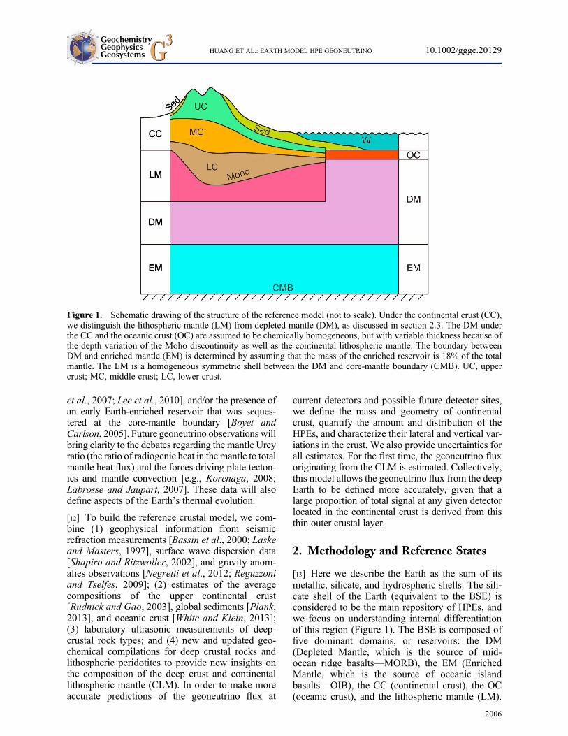
[13] Here we describe the Earth as the sum of itsmetallic, silicate, and hydrospheric shells. The sili-cate shell of the Earth (equivalent to the BSE) isconsidered to be the main repository of HPEs, andwe focus on understanding internal differentiationof this region (Figure 1). The BSE is composed offive dominant domains, or reservoirs: the DM(Depleted Mantle, which is the source of mid-ocean ridge basalts—MORB), the EM (EnrichedMantle, which is the source of oceanic islandbasalts—OIB), the CC (continental crust), the OC(oceanic crust), and the lithospheric mantle (LM).

Figure 1. Schematic drawing of the structure of the reference model (not to scale). Under the continental crust (CC),we distinguish the lithospheric mantle (LM) from depleted mantle (DM), as discussed in section 2.3. The DM underthe CC and the oceanic crust (OC) are assumed to be chemically homogeneous, but with variable thickness because ofthe depth variation of the Moho discontinuity as well as the continental lithospheric mantle. The boundary betweenDM and enriched mantle (EM) is determined by assuming that the mass of the enriched reservoir is 18% of the totalmantle. The EM is a homogeneous symmetric shell between the DM and core-mantle boundary (CMB). UC, uppercrust; MC, middle crust; LC, lower crust.

GeochemistryGeophysicsGeosystemsG3G3 HUANG ET AL.: EARTH MODEL HPE GEONEUTRINO 10.1002/ggge.20129

2006

Tab

le1.

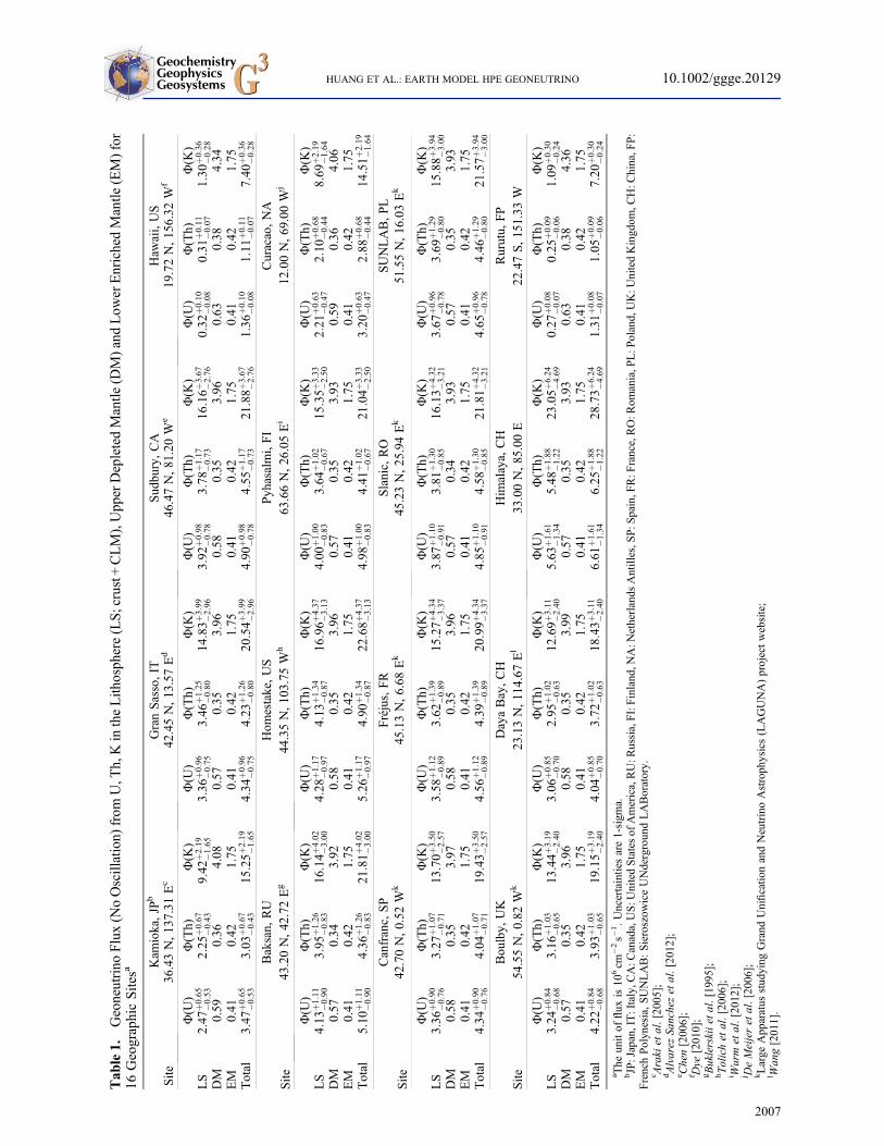
Geoneutrino

Flux(N

oOscillation)

from

U,T

h,KintheLith

osph

ere(LS;crust+CLM),Upp

erDepletedMantle

(DM)andLow

erEnrichedMantle

(EM)for

16GeographicSitesa

Site

Kam

ioka,JP

bGranSasso,IT

Sudbury,CA

Haw

aii,US

36.43N,137.31

Ec

42.45N,13.57Ed

46.47N,81.20W

e19.72N,156.32

Wf

Φ(U

)Φ(Th)

Φ(K

)Φ(U

)Φ(Th)

Φ(K

)Φ(U

)Φ(Th)

Φ(K

)Φ(U

)Φ(Th)

Φ(K

)LS

2:47

þ0:65

�0:53

2:25

þ0:67

�0:43

9:42

þ2:19

�1:65

3:36

þ0:96

�0:75

3:46

þ1:25

�0:80

14:83þ

3:99

�2:96

3:92

þ0:98

�0:78

3:78

þ1:17

�0:73

16:16þ

3:67

�2:76

0:32

þ0:10

�0:08

0:31

þ0:11

�0:07

1:30

þ0:36

�0:28

DM

0.59

0.36

4.08

0.57

0.35

3.96

0.58

0.35

3.96

0.63

0.38

4.34

EM

0.41

0.42

1.75

0.41

0.42

1.75

0.41

0.42

1.75

0.41

0.42

1.75

Total

3:47

þ0:65

�0:53

3:03

þ0:67

�0:43

15:25þ

2:19

�1:65

4:34

þ0:96

�0:75

4:23

þ1:26

�0:80

20:54þ

3:99

�2:96

4:90

þ0:98

�0:78

4:55

þ1:17

�0:73

21:88þ

3:67

�2:76

1:36

þ0:10

�0:08

1:11

þ0:11

�0:07

7:40

þ0:36

�0:28

Site

Baksan,

RU

Hom

estake,US

Pyhasalmi,FI

Curacao,NA

43.20N,42.72Eg

44.35N,103.75

Wh

63.66N,26.05Ei

12.00N,69.00W

j

Φ(U

)Φ(Th)

Φ(K

)Φ(U

)Φ(Th)

Φ(K

)Φ(U

)Φ(Th)

Φ(K

)Φ(U

)Φ(Th)

Φ(K

)LS

4:13

þ1:11

�0:90

3:95

þ1:26

�0:83

16:14þ

4:02

�3:00

4:28

þ1:17

�0:97

4:13

þ1:34

�0:87

16:96þ

4:37

�3:13

4:00

þ1:00

�0:83

3:64

þ1:02

�0:67

15:35þ

3:33

�2:50

2:21

þ0:63

�0:47

2:10

þ0:68

�0:44

8:69

þ2:19

�1:64

DM

0.57

0.34

3.92

0.58

0.35

3.96

0.57

0.35

3.93

0.59

0.36

4.06

EM

0.41

0.42

1.75

0.41

0.42

1.75

0.41

0.42

1.75

0.41

0.42

1.75

Total

5:10

þ1:11

�0:90

4:36

þ1:26

�0:83

21:81þ

4:02

�3:00

5:26

þ1:17

�0:97

4:90

þ1:34

�0:87

22:68þ

4:37

�3:13

4:98

þ1:00

�0:83

4:41

þ1:02

�0:67

21:04þ

3:33

�2:50

3:20

þ0:63

�0:47

2:88

þ0:68

�0:44

14:51þ

2:19

�1:64

Site

Canfranc,SP

Fréjus,FR

Slanic,RO

SUNLAB,PL

42.70N,0.52

Wk

45.13N,6.68

Ek

45.23N,25.94Ek

51.55N,16.03Ek

Φ(U

)Φ(Th)

Φ(K

)Φ(U

)Φ(Th)

Φ(K

)Φ(U

)Φ(Th)

Φ(K

)Φ(U

)Φ(Th)

Φ(K

)LS

3:36

þ0:90

�0:76

3:27

þ1:07

�0:71

13:70þ

3:50

�2:57

3:58

þ1:12

�0:89

3:62

þ1:39

�0:89

15:27þ

4:34

�3:37

3:87

þ1:10

�0:91

3:81

þ1:30

�0:85

16:13þ

4:32

�3:21

3:67

þ0:96

�0:78

3:69

þ1:29

�0:80

15:88þ

3:94

�3:00

DM

0.58

0.35

3.97

0.58

0.35

3.96

0.57

0.34

3.93

0.57

0.35

3.93

EM

0.41

0.42

1.75

0.41

0.42

1.75

0.41

0.42

1.75

0.41

0.42

1.75

Total

4:34

þ0:90

�0:76

4:04

þ1:07

�0:71

19:43þ

3:50

�2:57

4:56

þ1:12

�0:89

4:39

þ1:39

�0:89

20:99þ

4:34

�3:37

4:85

þ1:10

�0:91

4:58

þ1:30

�0:85

21:81þ

4:32

�3:21

4:65

þ0:96

�0:78

4:46

þ1:29

�0:80

21:57þ

3:94

�3:00

Site

Boulby,

UK

DayaBay,CH

Him

alaya,CH

Rurutu,

FP

54.55N,0.82

Wk

23.13N,114.67

El

33.00N,85.00E

22.47S,151.33

W

Φ(U

)Φ(Th)

Φ(K

)Φ(U

)Φ(Th)

Φ(K

)Φ(U

)Φ(Th)

Φ(K

)Φ(U

)Φ(Th)

Φ(K

)LS

3:24

þ0:84

�0:68

3:16

þ1:03

�0:65

13:44þ

3:19

�2:40

3:06

þ0:85

�0:70

2:95

þ1:02

�0:63

12:69þ

3:11

�2:40

5:63

þ1:61

�1:34

5:48

þ1:88

�1:22

23:05þ

6:24

�4:69

0:27

þ0:08

�0:07

0:25

þ0:09

�0:06

1:09

þ0:30

�0:24

DM

0.57

0.35

3.96

0.58

0.35

3.99

0.57

0.35

3.93

0.63

0.38

4.36

EM

0.41

0.42

1.75

0.41

0.42

1.75

0.41

0.42

1.75

0.41

0.42

1.75

Total

4:22

þ0:84

�0:68

3:93

þ1:03

�0:65

19:15þ

3:19

�2:40

4:04

þ0:85

�0:70

3:72

þ1:02

�0:63

18:43þ

3:11

�2:40

6:61

þ1:61

�1:34

6:25

þ1:88

�1:22

28:73þ

6:24

�4:69

1:31

þ0:08

�0:07

1:05

þ0:09

�0:06

7:20

þ0:30

�0:24

a The

unitof

flux

is10

6cm

�2s�

1.Uncertaintiesare1-sigm

a.bJP:Japan,IT:Italy,C

A:C

anada,US:U

nitedStatesof

America,RU:R

ussia,FI:Finland,N

A:N

etherlands

Antilles,S

P:S

pain,F

R:F

rance,RO:R

omania,P

L:P

oland,UK:U

nitedKingdom

,CH:C

hina,F

P:

FrenchPolynesia,SUNLAB:Sieroszow

iceUNdergroundLABoratory.

c Araki

etal.[2005];

dAlvarez

Sanchezet

al.[2012];

e Chen[2006];

f Dye

[2010];

gBuklerskiiet

al.[1995];

hTolichet

al.[2006];

i Wurm

etal.[2012];

j DeMeijeret

al.[2006];

kLarge

Apparatus

studying

Grand

Unificatio

nandNeutrinoAstrophysics(LAGUNA)projectwebsite;

l Wang[2011].

GeochemistryGeophysicsGeosystemsG3G3 HUANG ET AL.: EARTH MODEL HPE GEONEUTRINO 10.1002/ggge.20129

2007

It follows that BSE=DM+EM+CC+OC+LM.The modern convecting mantle is composed of theDM and the EM. We do not include a term for ahidden reservoir, which may or may not exist inthe BSE; its potential existence is not a consider-ation of this paper.

2.1. Selection of Flux Calculation Sites

[14] Although geoneutrinos can be measured, inprinciple, anywhere on the Earth, the experimentsneed to be carried out in underground (or underwa-ter) laboratories in order to shield detectors fromcosmic radiation; only a few locations thereforehave particular experimental interest. We havecalculated the fluxes at 16 sites where the explora-tion of the Earth through geoneutrinos is either cur-rently underway (Kamioka, Japan, with theKamLAND experiment [Araki et al., 2005; Gandoet al., 2011, 2013]; Gran Sasso, Italy, with theBorexino experiment [Alvarez Sanchez et al.,2012]; Sudbury, Ontario, Canada, with the SNO+experiment [Chen, 2006]), or where such experi-ments have been proposed or could be planned (Ta-ble 1). Hawaii (Hanohano) [Dye, 2010], Baksan(Baksan Neutrino Observatory) [Buklerskii et al.,1995], Homestake (Deep Underground Science andEngineering Laboratory) [Tolich et al., 2006],Curacao (Earth AntineutRino Tomography) [DeMeijer et al., 2006], and Daya Bay (Daya Bay II)[Wang, 2011] are all sites that have been proposedfor constructing liquid scintillator detectors capableof detecting geoneutrinos. LAGUNA (Large Appara-tus studying Grand Unification and Neutrino Astro-physics) is looking for the best site in Europe wherethe LENA (Low Energy Neutrino Astronomy) ex-periment [Wurm et al., 2012] could be built: sevenprospective underground sites in Europe (Pyhasalmi,Boulby, Canfranc, Fréjus, Slanic, and SUNLAB (seeLAGUNA website)) are being investigated. Finally,we also include the sites where the maximum andminimum geoneutrinos signal on the Earth’ssurface is expected: the Himalaya and Rurutu Island(Pacific Ocean), respectively.

2.2. Structure and Mass of the Crust

[15] In 1998, the CRUST 5.1 model [Mooney et al.,1998] was published as a refinement of the previous3SMAC model [Nataf and Richard, 1996]. Themodel included 2592 voxels on a 5� � 5� grid andreported the thickness and physical properties ofall ice and sediment accumulations and of normaland anomalous oceanic crust. Vast continentalregions (large portions of Africa, South America,

Antarctica, and Greenland) lacked direct observa-tions, and the predictions for these areas wereobtained by extrapolation based on the crustal struc-ture. Taking advantage of a compilation of newreflection and refraction seismic data, a global crustalmodel at 2� � 2� resolution (CRUST 2.0) by Bassinet al. [2000] provided an update to CRUST 5.1. Thismodel incorporates 16,200 crustal voxels and 360key profiles that contain the thickness, density andvelocity of compressional (Vp) and shear waves(Vs) for seven layers (ice, water, soft sediments, hardsediments, upper, middle, and lower crust) in eachvoxel. The Vp values are based on field measure-ments, while Vs and density are estimated by usingempirical Vp-Vs and Vp-density relationships,respectively [Mooney et al., 1998]. For regions lack-ing field measurements, the seismic velocity structureof the crust is extrapolated from the average crustalstructure for regions with similar crustal age and tec-tonic setting [Bassin et al., 2000]. Topography andbathymetry are adopted from a standard database(ETOPO-5). The same physical and elastic parame-ters are reported in a global sediment map digitizedon a 1� � 1� grid [Laske and Masters, 1997]. Theaccuracies of these models are not specified, and theymust vary with location and data coverage.

[16] The crust in our reference Earth model is com-posed of 64,800 voxels at a resolution of 1� � 1�and is divided into two main reservoirs: oceaniccrust (OC) and continental crust (CC). In the OC,we include the oceanic plateaus and the melt-affected oceanic crust of Bassin et al. [2000]. Theother crustal types identified in CRUST 2.0 are con-sidered to be CC, including oceanic plateaus com-prised of continental crust (the so-called “W” tilesof Bassin et al. [2000]), which are mainly foundin the north of the Scotia Plate, in the SeychellesPlate, in the plateaus around New Zealand(Campbell Plateau, Challenger Plateau, Lord HoweRise, and Chatham Rise), and on the northwestEuropean continental shelf. For each voxel, weadopt the physical information (density and relativethickness) of three sediment layers from the globalsediment map [Laske and Masters, 1997]; forupper, middle, and lower crust, we adopt the phys-ical and elastic parameters (Vp and Vs) fromCRUST 2.0 [Bassin et al., 2000].

[17] Evaluation of the uncertainties of the crustalstructure is complex, as the physical parameters(thickness, density, Vp, and Vs) are correlated,and their direct measurements are inhomogeneousover the globe [Mooney et al., 1998]. Seismicvelocities generally have smaller relative uncer-tainties than thickness [Christensen and Mooney,

GeochemistryGeophysicsGeosystemsG3G3 HUANG ET AL.: EARTH MODEL HPE GEONEUTRINO 10.1002/ggge.20129

2008

1995], since seismic velocities (Vp) are measureddirectly in the refraction method, while the depthsof refracting horizons are successively calculatedfrom the uppermost to the deepest layer measured.The uncertainties of seismic velocities in someprevious global crustal models were estimated tobe 3–4% [Holbrook et al., 1992; Mooney et al.,1998]. To be conservative, we adopt 5% (1-sigma)uncertainties for both Vp and Vs in our referencecrustal model.

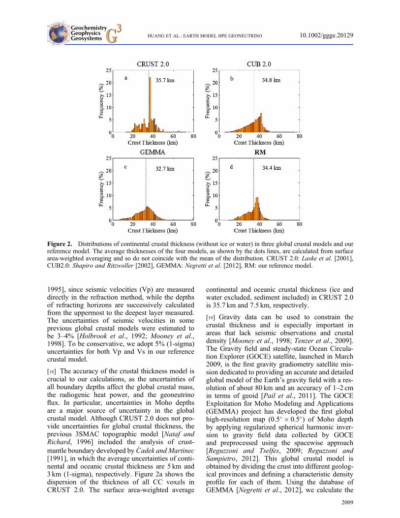
[18] The accuracy of the crustal thickness model iscrucial to our calculations, as the uncertainties ofall boundary depths affect the global crustal mass,the radiogenic heat power, and the geoneutrinoflux. In particular, uncertainties in Moho depthsare a major source of uncertainty in the globalcrustal model. Although CRUST 2.0 does not pro-vide uncertainties for global crustal thickness, theprevious 3SMAC topographic model [Nataf andRichard, 1996] included the analysis of crust-mantle boundary developed by �Cadek and Martinec[1991], in which the average uncertainties of conti-nental and oceanic crustal thickness are 5 km and3 km (1-sigma), respectively. Figure 2a shows thedispersion of the thickness of all CC voxels inCRUST 2.0. The surface area-weighted average

continental and oceanic crustal thickness (ice andwater excluded, sediment included) in CRUST 2.0is 35.7 km and 7.5 km, respectively.

[19] Gravity data can be used to constrain thecrustal thickness and is especially important inareas that lack seismic observations and crustaldensity [Mooney et al., 1998; Tenzer et al., 2009].The Gravity field and steady-state Ocean Circula-tion Explorer (GOCE) satellite, launched in March2009, is the first gravity gradiometry satellite mis-sion dedicated to providing an accurate and detailedglobal model of the Earth’s gravity field with a res-olution of about 80 km and an accuracy of 1–2 cmin terms of geoid [Pail et al., 2011]. The GOCEExploitation for Moho Modeling and Applications(GEMMA) project has developed the first globalhigh-resolution map (0.5� � 0.5�) of Moho depthby applying regularized spherical harmonic inver-sion to gravity field data collected by GOCEand preprocessed using the spacewise approach[Reguzzoni and Tselfes, 2009; Reguzzoni andSampietro, 2012]. This global crustal model isobtained by dividing the crust into different geolog-ical provinces and defining a characteristic densityprofile for each of them. Using the database ofGEMMA [Negretti et al., 2012], we calculate the

Figure 2. Distributions of continental crustal thickness (without ice or water) in three global crustal models and ourreference model. The average thicknesses of the four models, as shown by the dots lines, are calculated from surfacearea-weighted averaging and so do not coincide with the mean of the distribution. CRUST 2.0: Laske et al. [2001],CUB2.0: Shapiro and Ritzwoller [2002], GEMMA: Negretti et al. [2012], RM: our reference model.

GeochemistryGeophysicsGeosystemsG3G3 HUANG ET AL.: EARTH MODEL HPE GEONEUTRINO 10.1002/ggge.20129

2009

surface area-weighted average thicknesses of CCand OC to be 32.7 km and 8.8 km, respectively(Figure 2b).

[20] Another way to evaluate the global crustalthickness is by utilizing the phase and group veloc-ity measurements of the fundamental mode ofRayleigh and Love waves. Shapiro and Ritzwoller[2002] used a Monte Carlo method to invert surfacewave dispersion data for a global shear-velocitymodel of the crust and upper mantle on a 2� � 2�grid (CUB 2.0), with a priori constraints (includingdensity) from the CRUST 5.1 model [Mooneyet al., 1998]. With the data set of this model(courtesy of V. Lekic), the surface area-weightedaverage thicknesses of the CC and OC are34.8 km and 7.6 km, respectively (Figure 2c).

[21] The three global crustal models described abovewere obtained by different approaches, and the con-straints on the models are slightly dependent. Ideally,the best solution for a geophysical global crustalmodel is to combine data from different approaches:reflection and refraction seismic body wave, surfacewave dispersion, and gravimetric anomalies. In ourreference model, the thickness and its associated un-certainty of each 1� � 1� crustal voxel is obtained asthe mean and the half-range of the three models. Thesurface area-weighted average thicknesses of CC andOC are 34.4� 4.1 km (Figure 2d) and 8.0� 2.7 km(1-sigma) for our reference crustal model, respec-tively. The uncertainties reported here are not basedon the dispersions of thicknesses of CC and OCvoxels but are the surface area-weighted average ofuncertainties of each voxel’s thickness. Our esti-mated average CC thickness is about 16% less than41 km determined previously by Christensen andMooney [1995, see their Figure 2] on the basis ofavailable seismic refraction data at that time andassignment of crustal type sections for areas thatwere not sampled seismically. However, their compi-lation did not include continental margins, nor sub-merged continental platforms, which are included inthe three global crustal models used here. Inclusionof these areas will make the CC thinner, on average,than that based solely on exposed continents.

[22] Adopting from CRUST 2.0 the well-establishedthicknesses of water and ice, and the densities andrelative proportions of each crustal layer, we calcu-late the masses of all crustal layers, including thebulk CC and OC (Table 3). Summing the masses ofsediment, upper, middle, and lower crust, the totalmasses of CC and OC are estimated to be MCC=(20.6� 2.5)� 1021 kg and MOC= (6.7� 2.3)� 1021

kg (1-sigma). Thus, the fractional mass contribution

to the BSE of the CC is 0.51%, and the contributionof the OC is 0.17%. The uncertainty of crustal thick-ness of each voxel is dependent on that of othervoxels, but with undeterminable correlation, due tothe fact that the three crustal models are mutuallydependent, and the estimates of crustal thicknessesfor some voxels are extrapolated from the others.Considering these complexities, we make the conser-vative assumption that the uncertainty of Mohodepth in each voxel is totally dependent on thatof all the others. Compared to the total crustal mass(i.e., CC+OC) derived directly from CRUST 2.0(27.9� 1021 kg) [Dye, 2010], the total crustal massin our reference model ((27.3� 4.8)� 1021 kg) is~2% lower, but within uncertainty. Although theCC covers only ~40% of the Earth’s surface, itrepresents ~75% of the crustal mass; it is also thereservoir with the highest concentration of HPEs.Uncertainties in the concentrations of HPEs play aprominent role in constraining the crustal radiogenicheat power and geoneutrino flux, as discussed insection 6.

2.3. The Lithospheric Mantle

[23] Previous models of geoneutrino flux [Dye, 2010;Enomoto et al., 2007; Fogli et al., 2006; Mantovaniet al., 2004] have relied on CRUST 2.0 and thedensity profile of the mantle, as given by PREM (Pre-liminary Reference Earth Model, a 1-D seismo-logically based global model) [Dziewonski andAnderson, 1981]. In these models, the crust and themantle were treated as two separate geophysical andgeochemical reservoirs. In particular, the mantle wasconventionally described as a shell between the crustand the core and considered compositionally homo-geneous [Dye, 2010; Enomoto et al., 2007]. Thesemodels did not consider the heterogeneous topogra-phy of the base of the crust, or the likely differencesin composition of the lithospheric mantle underlyingthe oceanic and continental crusts.

[24] We treat the LM beneath the continents as a dis-tinct geophysical and geochemical reservoir that iscoupled to the crust in our reference Earth model(Figure 1). We assume that the LM beneath theoceans is compositionally identical to DM, and there-fore, we make no attempt to constrain its thickness.The thickness of the CLM is variable under eachcrustal voxel, with the top corresponding to theMohosurface and the bottom being difficult to constrain[Artemieva, 2006; Conrad and Lithgow-Bertelloni,

1Additional supporting information may be found in the onlineversion of this article.

GeochemistryGeophysicsGeosystemsG3G3 HUANG ET AL.: EARTH MODEL HPE GEONEUTRINO 10.1002/ggge.20129

2010

2006; Gung et al., 2003; Pasyanos, 2010]. Theseismically, thermally, and rheologically defineddepth to the base of the lithosphere may not be thesame [Jaupart and Mareschal, 1999; Jaupart et al.,1998; Jordan, 1975; Rudnick and Nyblade, 1999],and the thickness of the lithosphere can vary signifi-cantly across tectonic provinces, ranging from about100 km in areas affected by Phanerozoic tectonism,to ≥250 km in stable cratonic regions [Artemieva,2006; Pasyanos, 2010]. Here, we adopt 175� 75km(half-range uncertainty; 1-sigma) as representativeof the average depth to the base of CLM.

[25] The composition of the CLM is taken from anupdated database of xenolithic peridotite composi-tions [McDonough, 1990] (section D, DOI:10.1594/IEDA/100247 in the Supporting Informa-tion).1 The density profile of CLM under eachcrustal voxel is calculated using the linear parame-terization described in PREM. The mass of CLMis reported in Table 3; the main source of uncer-tainty comes from the average depth of the baseof CLM, while the uncertainty on Moho depthgives a negligible contribution.

2.4. The Sublithospheric Mantle

[26] Deeper in the Earth, direct observations de-crease dramatically, particularly, direct samplingof rocks for which geochemical data may beobtained. On the other hand, geoneutrinos are anextraordinary probe of the deep Earth. These parti-cles carry to the surface information about thechemical composition of the whole planet, and,in comparison with other emissions of the planet(e.g., heat or noble gases), they escape freely andinstantaneously from the Earth’s interior.

[27] The structure of mantle between the base oflithosphere and the core-mantle boundary (CMB)has been a topic of great debate. Tomographicimages of subducting slabs suggest deep mantleconvection [e.g., van der Hilst et al., 1997], whilesome geochemical observations favor a physicallyand chemically distinct upper and lower mantle,separated by the transition zone at the 660 km seis-mic discontinuity [e.g., Kramers and Tolstikhin,1997; Turcotte et al., 2001]. Within the geochemi-cal community, there is considerable disagreementregarding the composition of the upper and lowermantle [Allègre et al., 1996; Boyet and Carlson,2005; Javoy et al., 2010; McDonough and Sun,1995; Murakami et al., 2012].

[28] Evaluation of the detailed structure of the mantleis not a priority of this paper, and in our model, we

divide the sublithospheric mantle into two reservoirsthat are considered homogeneous. For simplicity,we assume these to be the depleted mantle (DM),which is on the top, and the underlying sphericallysymmetrical enriched mantle (EM) (Figure 1). TheDM is the source region for MORB, which provideconstraints on its chemical composition [Arevaloand McDonough, 2010; Arevalo et al., 2009]. TheDM under CC and OC is variable in thickness dueto the variable lithospheric thicknesses (Figure 1).The EM is an enriched reservoir beneath the DM,and the boundary between the two reservoirs,extending up to 710 km above the CMB, is estimatedby assuming that EM accounts 18% of the total massof the mantle [Arevalo et al., 2009; Arevalo et al.,2013]. The abundances of HPEs in the DM is 10times less than the global averageMORB abundances[Arevalo and McDonough, 2010]; the enrichmentfactor of EM over DM is estimated through a massbalance of HPEs in the mantle, assuming a BSEcomposition of McDonough and Sun [1995]. Thecompositions of the DM and EM (without any associ-ated uncertainties) are reported in Table 3. Šrámeket al. [2013] provide a detailed assessment of howdifferent geophysical and geochemical mantle modelsinfluence the calculated geoneutrino fluxes fromEarth’s mantle.

[29] The masses of DM and EM in our referencemodel (Table 3) are calculated by modeling the man-tle density profile using the coefficients of the poly-nomials reported in PREM in spherical symmetry.The total mantle mass is well-known, based on theterrestrial moment of inertia and the density-depthprofile of the Earth [Yoder, 1995]. The total massof the mantle in our model (CLM+DM+EM) is4.01� 1024 kg, in good agreement with thevalues reported by Anderson [2007] and Yoder[1995]. These results, combined with assumedabundances of HPEs in different reservoirs, willbe used in the following sections to predict thegeoneutrino flux and the global radiogenic heatpower of the Earth.

3. Compositions of Earth Reservoirs

[30] Here we review assumptions, definitions, anduncertainties in modeling the structure and com-position of all reservoirs in the reference modelexcept for the deep CC and CLM, for which wederive new estimates based on several new andupdated databases, as described in section 4.First-order constraints on the Earth’s structureare taken from PREM and a model for the

GeochemistryGeophysicsGeosystemsG3G3 HUANG ET AL.: EARTH MODEL HPE GEONEUTRINO 10.1002/ggge.20129

2011

composition of the Earth [McDonough, 2003;McDonough and Sun, 1995]. Beyond that, weconsider other input models and their associateduncertainties (Table 3).

3.1. The Core

[31] Following the discussion in McDonough[2003], the Earth’s core is considered to have neg-ligible amounts of K, Th, and U.

3.2. BSE Models and Uncertainties

[32] A first step in determining the compositions ofDM and EM in the reference model is to determinethe composition of the BSE. Methods used to esti-mate the amount of K, Th, and U in the BSE areprincipally based on cosmochemical, geochemical,and/or geodynamical data. Estimates based on U,a proxy for the total heat production in the planet,given planetary ratios of Th/U ~4 and K/U ~104,differs by almost a factor of 3 in the absolute HPEmasses in the BSE, i.e., between 0.5� 1017 and1.3� 1017 kg [Šrámek et al., 2013].

[33] A cosmochemical estimate for the BSE, whichyields the lowest U concentration, matches theEarth’s composition to a certain class of chondriticmeteorites, the enstatite chondrites. Javoy et al.[2010] and Warren [2011] noted the similarity inchemical and isotopic composition betweenenstatite chondrites and the Earth. Javoy et al.[2010] constructed an Earth model from thesechondritic building blocks and concluded that theBSE has a markedly low U content (i.e., 12 ng/gor 0.5� 1017 kg) and a total radiogenic heatproduction of 11 TW, using their preferred Th/Uof 3.6 and K/U of 11,000. This model requires thatthe lower two thirds of the mantle is enriched insilica, has a markedly lower Mg/Si value and differ-ent mineralogical composition than that of theupper mantle [e.g., Murakami et al., 2012], andthat the bulk of the HPEs is concentrated in theCC. However, large-scale, vertical differences inthe upper and lower mantle composition are seem-ingly inconsistent with seismological evidence forsubducting oceanic plates plunging into the deepmantle and stirring the entire convecting mantle.

[34] A BSE model with similarly low HPEs wasproposed by O’Neill and Palme [2008]. This modelhas only about 10 ng/g (i.e., 0.4� 1017 kg) of Ubased on the budget balance argument for the142Nd and 4He flux, and it invokes the loss of upto half of the planetary budget of Th and U (andother highly incompatible elements) due to

collisional erosion processes shortly followingEarth accretion. The major concern with modelsthat predict the BSE as having low overall HPEabundances is that this requires low radiogenic heatproduction in the mantle; the modern mantle isexpected to have only ~3 ng/g of U and ~3 TW ofradiogenic power, with the remaining fraction con-centrated in the CC.

[35] A geochemical method for modeling the BSEuses a combined approach of geochemical, petro-logic, and cosmochemical data to deconvolve thecompositional data from the mantle and crustalsamples [e.g., McDonough and Sun, 1995; Palmeand O’Neill, 2003]. These models predict about~0.8� 1017 kg U (i.e., ~20 ng/g) in the BSE, havea relatively homogeneous major element composi-tion throughout the mantle, and are consistent withelasticity models of the mantle and broader chon-dritic compositional models of the planet. Beingbased on samples, this method suffers from the factthat we may not sample the entire BSE and thusmay not identify all components in the mantle.

[36] The third approach to estimating the HPEs inthe BSE is based on the surface heat flux andderives solutions to the thermal evolution of theplanet by examining the relative contributions ofprimordial heat and heat production needed tomaintain a reasonable fit to the secular coolingrecord [e.g., Anderson, 2007; Turcotte and Schubert,2002]; the compositions derived using this methodare referred to here as geodynamical models. Suchgeodynamical models predict up to ~1.2� 1017 kgU (~30 ng/g) in the BSE and require that more than50% of the present heat flow is produced by radioac-tive decay. Defining the convective state of the man-tle in terms of Rayleigh convection, these modelscompare the force balance between buoyancy andviscosity, versus that between thermal and momen-tum diffusivities, and conclude that conditions inthe mantle greatly exceed the critical Rayleighnumber for the body, which marks the onset of con-vection. Thesemodels, however, also require markeddifferences in the chemical and mineralogical com-position of the upper and lower mantle but differfrom that of the cosmochemical models. A higherU content for the mantle translates into higher Caand Al contents (i.e., higher clinopyroxene andgarnet in the upper mantle or higher Ca-perovskitein the lower mantle), along with the rest of therefractory elements [McDonough and Sun, 1995],which, in turn, requires that the lower mantle has ahigher basaltic component than envisaged for theupper mantle.

GeochemistryGeophysicsGeosystemsG3G3 HUANG ET AL.: EARTH MODEL HPE GEONEUTRINO 10.1002/ggge.20129

2012

3.3. Sublithospheric Mantle (DM and EM)

[37] Here we adopt the model of McDonough andSun [1995] for the BSE, with updates for the absoluteHPE contents given in Arevalo et al. [2009]. In addi-tion, we use the definitions given by Arevalo et al.[2009] for the modern mantle, which is composedof two domains: a depleted mantle, DM, and a lowerenriched mantle, EM. We envisage no gross compo-sitional differences in major elements between thetwo domains, although the lowermost portion of themantle is assumed to be the source for OIB magmasand is consequently enriched in incompatible ele-ments (including HPEs) due to recycling of oceaniccrust [Hofmann and White, 1983].

3.4. Continental Lithospheric Mantle (CLM)

[38] The composition of the CLM adopted herestems from the earlier studies of McDonough[1990] and Rudnick et al. [1998], updated with newerliterature data (section 4). As described above, theCLM is taken as the region below the Moho to175� 75 km depth under the CC. These limits areset arbitrarily to cover the full range of variation seenin different locations, ~100 km in orogens and exten-sional regions and reaching ~250 km beneathcratons, but it allows for the inclusion of a CLM thatis likely to have a slight enrichment in HPEs due tosecondary processes (e.g., mantle metasomatism).A future goal of related studies is the incorporation ofgravimetric anomaly data and regional tomographicmodels, which may provide better geographicalresolution regarding the depth to the lithosphere-asthenosphere boundary.

3.5. Crustal Components, Compositions,and Uncertainties

[39] Compositional estimates for some portions ofthe crust are adopted from previous work, whereasthe composition of the deep continental crust isreevaluated in section 4.

3.5.1. Sediments

[40] We adopt the average composition of sedi-ments and reported uncertainties in the GlobalSubducting Sediments II model [Plank, 2013].

3.5.2. Oceanic Crust

[41] Areas in CRUST 2.0 labeled “A” and “B” arehere considered oceanic crust. We assume an aver-age oceanic crust composition as reported by Whiteand Klein [2013] and adopt a conservative

uncertainty of 30%. Seawater alteration can leadto enrichment of K and U in altered oceanic crust[Staudigel, 2003]. However, the oceanic crustmakes negligible contributions to the geoneutrinoflux and radiogenic heat power in the crust (Tables 2and 3), and increasing the U and K contents in theoceanic crust by a factor of 1.6, as suggested byPorter and White [2009], has no influence on theoutcomes of this study. We treat the three seismi-cally defined layers of basaltic oceanic crustreported by Mooney et al. [1998] as having thesame composition as average oceanic crust.

3.5.3. Upper Continental Crust

[42] We adopt the compositional model reported byRudnick and Gao [2003] for the upper continentalcrust and the uncertainties reported therein. Follow-ing Mooney et al. [1998], the upper continentalcrust is defined seismically as the uppermost crys-talline region in CRUST 2.0, having an averageVp of between 5.3 and 6.5 km s�1.

4. Refined Estimates for the Compositionof the Deep Continental Crust andContinental Lithospheric Mantle

4.1. General Considerations

[43] Given the large number of high-quality geo-chemical analyses now available for medium- tohigh-grade crustal metamorphic rocks, peridotites,ultrasonic laboratory velocity measurements, and,especially, the large numbers of seismic refractiondata for the crust (and their incorporation intoCRUST 2.0), we reevaluate here the compositionof the deep CC and lithospheric mantle.

[44] For the lithospheric mantle, we have updatedthe geochemical database for both massif and xeno-lithic peridotites of McDonough [1990] andRudnick et al. [1998], as detailed in section 4.3.2.For the deep CC, we follow the approach used byRudnick and Fountain [1995] and Christensenand Mooney [1995], who linked laboratory ultra-sonic velocity measurements to the geochemistryof various meta-igneous rocks. Laboratory mea-surements of Vp and Vs of both amphibolite andgranulite facies rocks are negatively correlated withtheir SiO2 contents (Figure 3). This correlation al-lows one to estimate the bulk chemical compositionof the lower and middle CC using seismic velocitydata [Christensen and Mooney, 1995; Rudnick andFountain, 1995].

GeochemistryGeophysicsGeosystemsG3G3 HUANG ET AL.: EARTH MODEL HPE GEONEUTRINO 10.1002/ggge.20129

2013

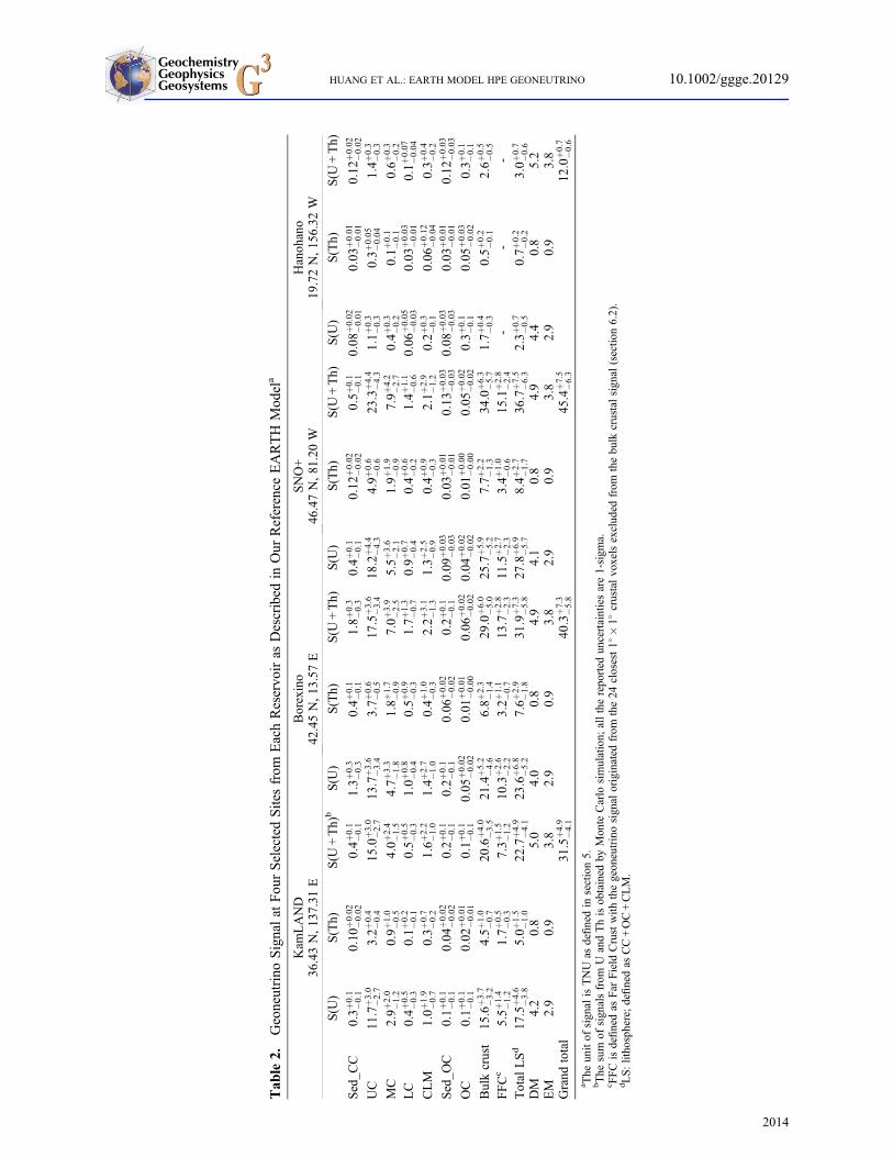
Tab

le2.

Geoneutrino

Signalat

Fou

rSelectedSitesfrom

EachReservo

iras

Described

inOur

Reference

EARTH

Mod

ela

Kam

LAND

Borexino

SNO+

Hanohano

36.43N,137.31

E42.45N,13.57E

46.47N,81.20W

19.72N,156.32

W

S(U

)S(Th)

S(U

+Th)

bS(U

)S(Th)

S(U

+Th)

S(U

)S(Th)

S(U

+Th)

S(U

)S(Th)

S(U

+Th)

Sed_C

C0:3þ

0:1

�0:1

0:10

þ0:02

�0:02

0:4þ

0:1

�0:1

1:3þ

0:3

�0:3

0:4þ

0:1

�0:1

1:8þ

0:3

�0:3

0:4þ

0:1

�0:1

0:12

þ0:02

�0:02

0:5þ

0:1

�0:1

0:08

þ0:02

�0:01

0:03

þ0:01

�0:01

0:12

þ0:02

�0:02

UC

11:7

þ3:0

�2:7

3:2þ

0:4

�0:4

15:0

þ3:0

�2:7

13:7

þ3:6

�3:4

3:7þ

0:6

�0:5

17:5

þ3:6

�3:4

18:2

þ4:4

�4:3

4:9þ

0:6

�0:6

23:3

þ4:4

�4:3

1:1þ

0:3

�0:3

0:3þ

0:05

�0:04

1:4þ

0:3

�0:3

MC

2:9þ

2:0

�1:2

0:9þ

1:0

�0:5

4:0þ

2:4

�1:5

4:7þ

3:3

�1:8

1:8þ

1:7

�0:9

7:0þ

3:9

�2:5

5:5þ

3:6

�2:1

1:9þ

1:9

�0:9

7:9þ

4:2

�2:7

0:4þ

0:3

�0:2

0:1þ

0:1

�0:1

0:6þ

0:3

�0:2

LC

0:4þ

0:5

�0:3

0:1þ

0:2

�0:1

0:5þ

0:5

�0:3

1:0þ

0:8

�0:4

0:5þ

0:9

�0:3

1:7þ

1:3

�0:7

0:9þ

0:7

�0:4

0:4þ

0:6

�0:2

1:4þ

1:1

�0:6

0:06

þ0:05

�0:03

0:03

þ0:03

�0:01

0:1þ

0:07

�0:04

CLM

1:0þ

1:9

�0:7

0:3þ

0:7

�0:2

1:6þ

2:2

�1:0

1:4þ

2:7

�1:0

0:4þ

1:0

�0:3

2:2þ

3:1

�1:3

1:3þ

2:5

�0:9

0:4þ

0:9

�0:3

2:1þ

2:9

�1:2

0:2þ

0:3

�0:1

0:06

þ0:12

�0:04

0:3þ

0:4

�0:2

Sed_O

C0:1þ

0:1

�0:1

0:04

þ0:02

�0:02

0:2þ

0:1

�0:1

0:2þ

0:1

�0:1

0:06

þ0:02

�0:02

0:2þ

0:1

�0:1

0:09

þ0:03

�0:03

0:03

þ0:01

�0:01

0:13

þ0:03

�0:03

0:08

þ0:03

�0:03

0:03

þ0:01

�0:01

0:12

þ0:03

�0:03

OC

0:1þ

0:1

�0:1

0:02

þ0:01

�0:01

0:1þ

0:1

�0:1

0:05

þ0:02

�0:02

0:01

þ0:01

�0:00

0:06

þ0:02

�0:02

0:04

þ0:02

�0:02

0:01

þ0:00

�0:00

0:05

þ0:02

�0:02

0:3þ

0:1

�0:1

0:05

þ0:03

�0:02

0:3þ

0:1

�0:1

Bulkcrust

15:6

þ3:7

�3:2

4:5þ

1:0

�0:7

20:6

þ4:0

�3:5

21:4

þ5:2

�4:6

6:8þ

2:3

�1:4

29:0

þ6:0

�5:0

25:7

þ5:9

�5:2

7:7þ

2:2

�1:3

34:0

þ6:3

�5:7

1:7þ

0:4

�0:3

0:5þ

0:2

�0:1

2:6þ

0:5

�0:5

FFCc

5:5þ

1:4

�1:2

1:7þ

0:5

�0:3

7:3þ

1:5

�1:2

10:3

þ2:6

�2:2

3:2þ

1:1

�0:7

13:7

þ2:8

�2:3

11:5

þ2:7

�2:3

3:4þ

1:0

�0:6

15:1

þ2:8

�2:4

--

-Total

LSd

17:5

þ4:6

�3:8

5:0þ

1:5

�1:0

22:7

þ4:9

�4:1

23:6

þ6:8

�5:2

7:6þ

2:9

�1:8

31:9

þ7:3

�5:8

27:8

þ6:9

�5:7

8:4þ

2:7

�1:7

36:7

þ7:5

�6:3

2:3þ

0:7

�0:5

0:7þ

0:2

�0:2

3:0þ

0:7

�0:6

DM

4.2

0.8

5.0

4.0

0.8

4.9

4.1

0.8

4.9

4.4

0.8

5.2

EM

2.9

0.9

3.8

2.9

0.9

3.8

2.9

0.9

3.8

2.9

0.9

3.8

Grand

total

31:5

þ4:9

�4:1

40:3

þ7:3

�5:8

45:4

þ7:5

�6:3

12:0

þ0:7

�0:6

a The

unitof

signal

isTNU

asdefinedin

section5.

bThe

sum

ofsignalsfrom

UandThisobtained

byMonte

Carlo

simulation;

allthereported

uncertaintiesare1-sigm

a.c FFCisdefinedas

Far

Field

Crustwith

thegeoneutrinosignal

originated

from

the24

closest1�

�1�

crustalvoxelsexcluded

from

thebulk

crustalsignal

(sectio

n6.2).

dLS:lithosphere;definedas

CC+OC+CLM.

GeochemistryGeophysicsGeosystemsG3G3 HUANG ET AL.: EARTH MODEL HPE GEONEUTRINO 10.1002/ggge.20129

2014

[45] Behn and Kelemen [2003], following Sobolevand Babeyko [1994], examined the relationshipbetween Vp and major elements abundances ofanhydrous igneous and meta-igneous rocks by mak-ing thermodynamic calculations of stable mineralassemblages for a variety of igneous rock composi-tions at deep crustal conditions and then calculatingtheir seismic velocities. They found a correlationbetween composition and seismic velocities but alsofound very broad compositional bounds for a specificVp in the deep CC and concluded that P-wave veloc-ities alone are insufficient to provide constraints on thedeep crustal composition. In particular, they noted thatin situ P-wave velocities in the lower crust of up to7.0 km/s (corresponding to room temperature and600MPa Vp of 7.14km/s calculated for an averagecrustal geotherm of 60mW/m2, using the temperaturederivative given below) may reflect granulite-faciesrocks having dacitic (~60wt% SiO2) compositions.However, such broad compositional bounds are notobserved in the laboratory data plotted in Figure 3.For example, the SiO2 content of rocks with Vp of~7.1 km/s ranges from 42 to 52wt% SiO2 for bothamphibolite and granulite-facies lithologies.

[46] We conclude that the correlation between seis-mic velocities and SiO2, and the range in velocitiesat a given SiO2 (Figure 3), allow quantitative esti-mates of deep crustal composition and associateduncertainties. In the next three sections, we de-scribe, in detail, the methodology employed here.

4.2. In Situ Velocity to Rock Type

[47] Ultrasonic compressional and shear wavevelocities have been determined for a variety ofcrustal rocks at different pressures and temperatures[e.g., Birch, 1960]. We have compiled publishedlaboratory seismic velocity data for deep crustal rocktypes and summarize their average seismic propertiesat a confining pressure of 0.6GPa and room temper-ature (section A, DOI: 10.1594/IEDA/100238;Figure 4; Table 4).

[48] Several selection criteria are applied to the dataset. The compilation includes only data for grain-boundary-fluid free and unaltered rocks whoselaboratory measurements were made in at leastthree orthogonal directions. We limit our compila-tion to measurements made at pressures ≥0.6GPain order to simulate pressures appropriate for thedeep crust. Complete or near-complete closure ofmicrocracks in the samples included in the compila-tion was ascertained by examining whether theseismic velocities increase linearly with pressureT

able

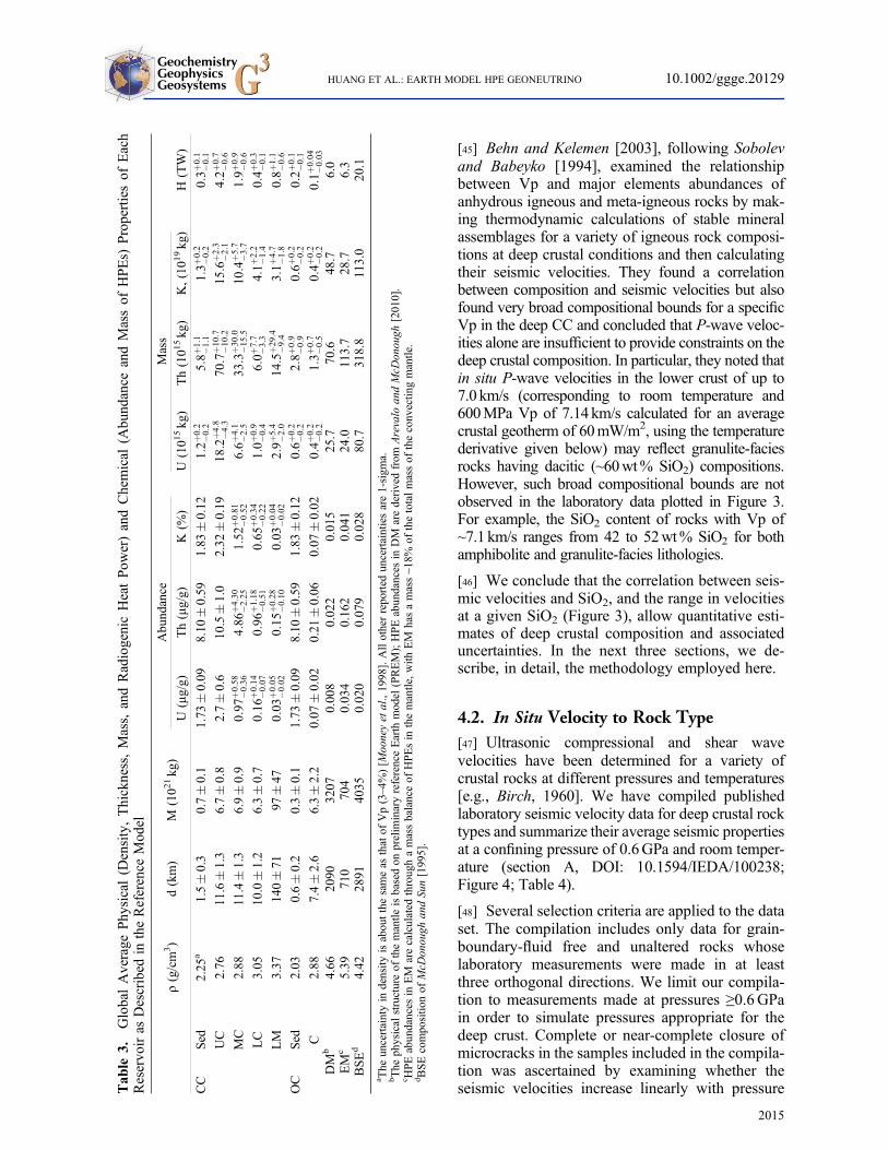
3.GlobalAverage

Phy

sical(D

ensity,Thickness,Mass,

andRadiogenicHeatPow

er)andChemical

(Abu

ndance

andMassof

HPEs)

Propertiesof

Each

Reservo

iras

Described

intheReference

Mod

el

r(g/cm

3)

d(km)

M(102

1kg)

Abundance

Mass

H(TW)

U(mg/g)

Th(mg/g)

K(%

)U

(101

5kg)

Th(101

5kg)

K,(101

9kg)

CC

Sed

2.25

a1.5�0.3

0.7�0.1

1.73

�0.09

8.10

�0.59

1.83

�0.12

1:2þ

0:2

�0:2

5:8þ

1:1

�1:1

1:3þ

0:2

�0:2

0:3þ

0:1

�0:1

UC

2.76

11.6�1.3

6.7�0.8

2.7�0.6

10.5�1.0

2.32

�0.19

18:2

þ4:8

�4:3

70:7

þ10:7

�10:2

15:6

þ2:3

�2:1

4:2þ

0:7

�0:6

MC

2.88

11.4�1.3

6.9�0.9

0:97

þ0:58

�0:36

4:86

þ4:30

�2:25

1:52

þ0:81

�0:52

6:6þ

4:1

�2:5

33:3

þ30:0

�15:5

10:4

þ5:7

�3:7

1:9þ

0:9

�0:6

LC

3.05

10.0�1.2

6.3�0.7

0:16

þ0:14

�0:07

0:96

þ1:18

�0:51

0:65

þ0:34

�0:22

1:0þ

0:9

�0:4

6:0þ

7:7

�3:3

4:1þ

2:2

�1:4

0:4þ

0:3

�0:1

LM

3.37

140�71

97�47

0:03

þ0:05

�0:02

0:15

þ0:28

�0:10

0:03

þ0:04

�0:02

2:9þ

5:4

�2:0

14:5

þ29:4

�9:4

3:1þ

4:7

�1:8

0:8þ

1:1

�0:6

OC

Sed

2.03

0.6�0.2

0.3�0.1

1.73

�0.09

8.10

�0.59

1.83

�0.12

0:6þ

0:2

�0:2

2:8þ

0:9

�0:9

0:6þ

0:2

�0:2

0:2þ

0:1

�0:1

C2.88

7.4�2.6

6.3�2.2

0.07

�0.02

0.21

�0.06

0.07

�0.02

0:4þ

0:2

�0:2

1:3þ

0:7

�0:5

0:4þ

0:2

�0:2

0:1þ

0:04

�0:03

DM

b4.66

2090

3207

0.008

0.022

0.015

25.7

70.6

48.7

6.0

EM

c5.39

710

704

0.034

0.162

0.041

24.0

113.7

28.7

6.3

BSEd

4.42

2891

4035

0.020

0.079

0.028

80.7

318.8

113.0

20.1

a The

uncertaintyin

density

isaboutthesameas

that

ofVp(3–4%)[M

ooneyet

al.,1998].Allotherreported

uncertaintiesare1-sigm

a.bThe

physical

structureof

themantle

isbasedon

prelim

inaryreferenceEarth

model

(PREM);HPEabundances

inDM

arederivedfrom

Arevalo

andMcD

onough

[2010].

c HPEabundances

inEM

arecalculated

throughamassbalanceof

HPEsin

themantle,with

EM

hasamass~1

8%of

thetotalmassof

theconvectin

gmantle.

dBSEcompositio

nof

McD

onough

andSun[1995].

GeochemistryGeophysicsGeosystemsG3G3 HUANG ET AL.: EARTH MODEL HPE GEONEUTRINO 10.1002/ggge.20129

2015

after reaching 0.4GPa. Physical properties ofxenoliths are usually significantly influenced byirreversible grain boundary alteration that occursduring entrainment [Parsons et al., 1995; Rudnickand Jackson, 1995]. Since such alteration is notlikely to be a feature of in situ deep crust, xenolithdata are excluded from our compilation.

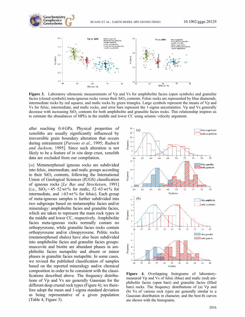
[49] Metamorphosed igneous rocks are subdividedinto felsic, intermediate, and mafic groups accordingto their SiO2 contents, following the InternationalUnion of Geological Sciences (IUGS) classificationof igneous rocks [Le Bas and Streckeisen, 1991](i.e., SiO2 = 45–52wt% for mafic, 52–63wt% forintermediate, and >63wt% for felsic). Each groupof meta-igneous samples is further subdivided intotwo subgroups based on metamorphic facies and/ormineralogy: amphibolite facies and granulite facies,which are taken to represent the main rock types inthe middle and lower CC, respectively. Amphibolitefacies meta-igneous rocks normally contain noorthopyroxene, while granulite facies rocks containorthopyroxene and/or clinopyroxene. Pelitic rocks(metamorphosed shales) have also been subdividedinto amphibolite facies and granulite facies groups:muscovite and biotite are abundant phases in am-phibolite facies metapelite and absent or minorphases in granulite facies metapelite. In some cases,we revised the published classification of samplesbased on the reported mineralogy and/or chemicalcomposition in order to be consistent with the classi-fications described above. The frequency distribu-tions of Vp and Vs are generally Gaussian for thedifferent deep crustal rock types (Figure 4); we there-fore adopt the mean and 1-sigma standard deviationas being representative of a given population(Table 4, Figure 3).

Figure 3. Laboratory ultrasonic measurements of Vp and Vs for amphibolite facies (open symbols) and granulitefacies (closed symbols) meta-igneous rocks versus their SiO2 contents. Felsic rocks are represented by blue diamonds,intermediate rocks by red squares, and mafic rocks by green triangles. Large symbols represent the means of Vp andVs for felsic, intermediate, and mafic rocks, and error bars represent the 1-sigma uncertainties. Vp and Vs generallydecrease with increasing SiO2 contents for both amphibolite and granulite facies rocks. This relationship inspires usto estimate the abundances of HPEs in the middle and lower CC using seismic velocity argument.

Figure 4. Overlapping histograms of laboratory-measured Vp and Vs of felsic (blue) and mafic (red) am-phibolite facies (open bars) and granulite facies (filledbars) rocks. The frequency distributions of (a) Vp and(b) Vs of various rock types are generally similar to aGaussian distribution in character, and the best-fit curvesare shown with the histograms.

GeochemistryGeophysicsGeosystemsG3G3 HUANG ET AL.: EARTH MODEL HPE GEONEUTRINO 10.1002/ggge.20129

2016

[50] Because seismic velocities of rocks in the deepcrust are strongly influenced by pressure and temper-ature, we correct the compiled laboratory-measuredvelocities for all rock groups (which were attainedat 0.6GPa and room temperature) to seismic veloci-ties appropriate for pressure-temperature conditionsin the deep crust. To compare our compiled labora-tory ultrasonic velocities to the velocities in thecrustal reference model, we apply pressure and tem-perature derivatives of 2� 10�4 km s�1MPa�1 and�4� 10�4 km s�1 �C�1, respectively, for both Vp

and Vs [Christensen and Mooney, 1995; Rudnickand Fountain, 1995] and assume a typical conduc-tive geotherm equivalent to a surface heat flow of60mW �m�2 [Pollack and Chapman, 1977]. Usingthe in situ Vp and Vs profiles for the middle(or lower) CC of each voxel given in CRUST 2.0,we estimate the fractions of felsic and mafic amphib-olite facies (or granulite facies) rocks by comparingthe in situ seismic velocities with the temperature-and pressure-corrected laboratory-measured veloci-ties under the assumption that the middle (or lower)

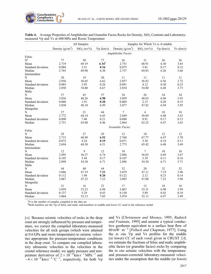
Table 4. Average Properties of Amphibolite and Granulite Facies Rocks for Density, SiO2 Contents and Laboratory-measured Vp and Vs at 600MPa and Room Temperature

All Samples Samples for Which Vs is Available

Density (g/cm3) SiO2 (wt%) Vp (km/s) Density (g/cm3) SiO2 (wt%) Vp (km/s) Vs (km/s)

Amphibolite FaciesFelsicNa 77 50 77 36 31 36 36Mean 2.719 69.19 6.34b 2.751 68.91 6.30 3.65Standard deviation 0.084 3.51 0.16 0.075 3.81 0.17 0.12Median 2.703 69.98 6.30 2.737 69.83 6.26 3.66IntermediateN 20 19 20 11 11 11 11Mean 2.856 56.65 6.62 2.857 56.83 6.56 3.72Standard deviation 0.085 3.95 0.26 0.091 4.12 0.30 0.23Median 2.850 54.80 6.67 2.854 54.80 6.48 3.73MaficN 57 43 57 34 26 34 34Mean 3.036 48.26 6.98 3.059 48.03 6.96 3.93Standard deviation 0.068 1.91 0.20 0.069 2.15 0.20 0.15Median 3.030 48.10 6.99 3.077 47.82 6.94 3.95MetapeliteN 27 21 44 7 4 18 18Mean 2.772 64.14 6.45 2.849 58.89 6.48 3.63Standard deviation 0.090 7.40 0.21 0.080 8.91 0.17 0.13Median 2.751 65.08 6.46 2.864 62.25 6.47 3.63

Granulite FaciesFelsicN 29 27 29 12 10 12 12Mean 2.715 68.89 6.52 2.760 67.77 6.47 3.70Standard deviation 0.072 4.24 0.19 0.071 5.38 0.18 0.11Median 2.694 68.30 6.51 2.773 65.42 6.48 3.69IntermediateN 12 9 12 10 7 10 10Mean 2.895 56.27 6.74 2.886 56.03 6.69 3.67Standard deviation 0.105 3.44 0.17 0.107 3.39 0.11 0.16Median 2.898 54.30 6.71 2.896 54.30 6.71 3.71MaficN 44 40 44 32 28 32 32Mean 3.066 47.19 7.21 3.079 47.11 7.19 3.96Standard deviation 0.112 1.98 0.20 0.122 2.12 0.23 0.14Median 3.067 47.23 7.23 3.085 47.00 7.23 3.98MetapeliteN 21 16 23 17 12 18 18Mean 3.059 53.23 6.98 3.067 53.31 6.90 3.99Standard deviation 0.137 5.29 0.43 0.150 5.89 0.43 0.18Median 3.064 52.13 7.03 3.074 52.13 6.97 3.99

aN is the number of samples compiled in the data set.bBold numbers are the Vp of felsic and mafic end-members in middle and lower CC used in the reference model.

GeochemistryGeophysicsGeosystemsG3G3 HUANG ET AL.: EARTH MODEL HPE GEONEUTRINO 10.1002/ggge.20129

2017

CC is a binary mixture of felsic and mafic end-members as defined by the following:

f þ m ¼ 1 (1)

f � vf þ m� vm ¼ vcrust (2)

where f and m are the mass fractions of felsic andmafic end-members in the middle (or lower) CC;vf, vm, and vcrust are Vp or Vs of the felsic and maficend-members (pressure- and temperature-corrected)and in the crustal layer, respectively. We use onlyVp to constrain the felsic fraction (f) in the middleor lower CC for three main reasons: using Vs givesresults for (f) in the deep crust that are in good agree-ment with those derived from the Vp data, the largeroverlap of Vs distributions for the felsic and maficend-members in the deep crust (Figure 4b) limitsits usefulness in distinguishing the two end-members, and Vs data in the crust are deduceddirectly from measured Vp data in CRUST 2.0.

[51] Intermediate composition meta-igneous rockshave intermediate seismic velocities compared tothose of felsic and mafic rocks; therefore, they arenot considered as a separate entity here. As pointedout by Rudnick and Fountain [1995], the very largerange in velocities for metapelitic sedimentaryrocks (metapelites) makes determination of theirdeep crustal abundances using seismic velocitiesimpossible. Here we assume that metapelites are anegligible component in the deep crust. Since theyhave higher abundances of HPEs than mafic rocksand similar HPE contents to felsic rocks, ignoringtheir presence may lead to an underestimation ofHPEs in the deep continental crust. Thus, our esti-mates should be regarded as minima.

[52] For room temperature and 600MPa pressure,amphibolite-facies felsic rocks have an averageVp of 6.34� 0.16 km/s (1-sigma) and a Vs of3.65� 0.12 km/s, while average mafic amphiboliteshave a Vp of 6.98� 0.20 km/s and a Vs of3.93� 0.15 km/s. Granulite-facies felsic rocks havean average Vp of 6.52� 0.19 km/s and a Vs of3.70� 0.11 km/s, while mafic granulites have anaverage Vp of 7.21� 0.20 km/s and a Vs of3.96� 0.14 km/s. Our new compilation yieldsaverage velocities that are consistent with previousestimates for similar rock types considered byChristensen and Mooney [1995] and Rudnick andFountain [1995] but provides a larger sample sizethan the latter study, due to more recently publishedlaboratory investigations. The sample size consideredhere is not as large as that reported byChristensen andMooney [1995], who incorporated many unpublishedresults that are not available to this study.

4.3. Rock Type to Chemistry

[53] New and updated compositional databases foramphibolite and granulite facies crustal rocks andmantle peridotites are used here (sections B (DOI:10.1594/IEDA/100245), C (DOI: 10.1594/IEDA/100246), and D) to derive a sample-driven estimateof the average composition of different regions ofthe continental lithosphere (e.g., amphibolite faciesfor middle CC, granulite facies for lower CC, andxenolithic peridotites for CLM). As with theultrasonic data compilation, several selectioncriteria were also applied to the geochemical datacompilation. Only data for whole rock samples thatwere accompanied by appropriate lithologicaldescriptions were used so that the metamorphicfacies of the sample could be properly assigned.X-ray fluorescence determinations of U and Thwere excluded due to generally poor data quality,and samples described as being weathered wereexcluded from the compilation. Finally, major ele-ment compositions of all rocks were normalized to100 wt% anhydrous, and the log-normal averagesof HPEs were adopted, following the recommenda-tion of Ahrens [1954], with uncertainties for the av-erage compositions representing the 1-sigma limits.

[54] In addition to the above considerations, intrinsicproblems associated with amassing such databases,particularly for peridotites, include the following[McDonough, 1990; Rudnick et al., 1998]:[55] 1. Overabundance of data from an individualstudy, region, or laboratory;[56] 2. Under-representation of some sample typesbecause of their intrinsically lower trace elementconcentrations (e.g., dunites), presenting a signi-ficant analytical challenge (lower limit of detectionproblems);[57] 3. Geological processes (e.g., magmatic en-trainment) are potentially nonrandom processes thatmay bias our overall view of the deeper portion ofthe lithosphere;[58] 4. Weathering can significantly affect theabundances of the mobile elements, particularly Kand U.

4.3.1. Deep Crust Composition

[59] The compositional databases for amphiboliteand granulite facies crustal rocks are bothsubdivided into felsic, intermediate, and maficmeta-igneous rocks based on the normalized SiO2

content and metasedimentary rocks. For each cate-gory, the frequency distributions of HPE abun-dances show ranges that span nearly four orders ofmagnitude and are strongly positively skewed,

GeochemistryGeophysicsGeosystemsG3G3 HUANG ET AL.: EARTH MODEL HPE GEONEUTRINO 10.1002/ggge.20129

2018

rather than Gaussian (Figure 5); they generally fit alog-normal distribution [Ahrens, 1954]. In order todecrease the influence of rare enriched or depletedsamples on the log-normal average chemicalcomposition for each category, we apply a 1.15-sigmafilter that removes ~25% of the data that fall beyondthese bounds and then calculate the centralvalues and associated 1-sigma uncertainties of HPEabundances based on the filtered data for eachcategory (see Supporting Information).

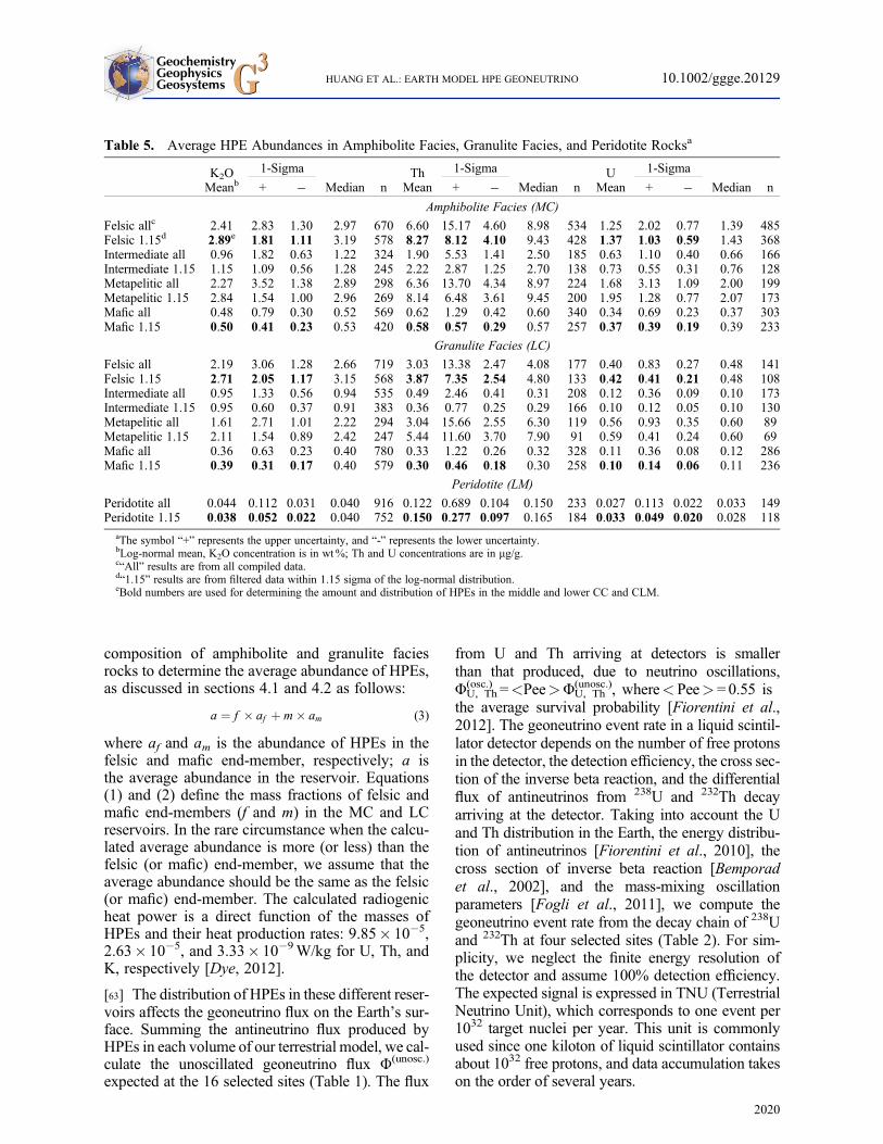
[60] The distributions of the HPE abundances infelsic and mafic amphibolite and granulite faciesrocks after such filtering are illustrated inFigure 6, and the results are reported in Table 5,along with associated 1-sigma uncertainties. Thesevalues are adopted in the reference model toestimate the HPE abundances in the heterogeneousmiddle and lower CC, as described in section 5.

4.3.2. Average Composition of Peridotitesand Uncertainties

[61] The peridotite database is subdivided into threecategories: spinel, garnet, and massif peridotites(section D). Spinel and garnet xenolithic peridotitesare assumed to represent the major rock types in theCLM, while massif peridotites are assumed to rep-resent lithospheric mantle under oceanic crust.Due to the analytical challenge of measuring lowU and Th concentrations in the lithospheric mantle,

there are only several tens of reliable measurementsavailable for statistical analyses of garnet andmassif peridotites. We apply the same data treat-ment (1.15-sigma filtering) to the peridotitedatabase, since distributions of HPEs of all thethree types of peridotites are positively skewedand fit the log-normal distribution better than nor-mal distribution. The log-normal mean valuesadopted in the reference model are close to themedian values of the database and provide robustand coherent estimates to the composition oflithospheric mantle (Table 5) [McDonough, 1990;Rudnick et al., 1998].

5. Methods of Analysis and Propagationof Uncertainties

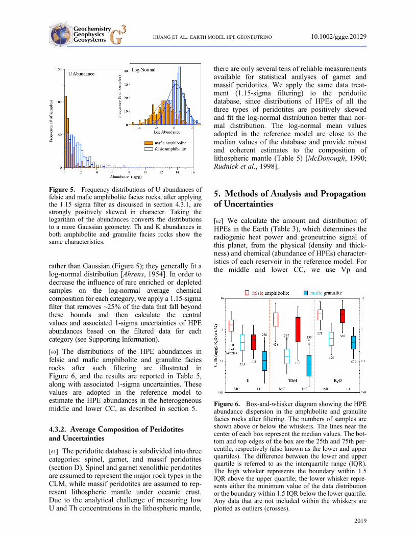
[62] We calculate the amount and distribution ofHPEs in the Earth (Table 3), which determines theradiogenic heat power and geoneutrino signal ofthis planet, from the physical (density and thick-ness) and chemical (abundance of HPEs) character-istics of each reservoir in the reference model. Forthe middle and lower CC, we use Vp and

Figure 5. Frequency distributions of U abundances offelsic and mafic amphibolite facies rocks, after applyingthe 1.15 sigma filter as discussed in section 4.3.1, arestrongly positively skewed in character. Taking thelogarithm of the abundances converts the distributionsto a more Gaussian geometry. Th and K abundances inboth amphibolite and granulite facies rocks show thesame characteristics.

Figure 6. Box-and-whisker diagram showing the HPEabundance dispersion in the amphibolite and granulitefacies rocks after filtering. The numbers of samples areshown above or below the whiskers. The lines near thecenter of each box represent the median values. The bot-tom and top edges of the box are the 25th and 75th per-centile, respectively (also known as the lower and upperquartiles). The difference between the lower and upperquartile is referred to as the interquartile range (IQR).The high whisker represents the boundary within 1.5IQR above the upper quartile; the lower whisker repre-sents either the minimum value of the data distributionor the boundary within 1.5 IQR below the lower quartile.Any data that are not included within the whiskers areplotted as outliers (crosses).

GeochemistryGeophysicsGeosystemsG3G3 HUANG ET AL.: EARTH MODEL HPE GEONEUTRINO 10.1002/ggge.20129

2019

composition of amphibolite and granulite faciesrocks to determine the average abundance of HPEs,as discussed in sections 4.1 and 4.2 as follows:

a ¼ f � af þ m� am (3)

where af and am is the abundance of HPEs in thefelsic and mafic end-member, respectively; a isthe average abundance in the reservoir. Equations(1) and (2) define the mass fractions of felsic andmafic end-members (f and m) in the MC and LCreservoirs. In the rare circumstance when the calcu-lated average abundance is more (or less) than thefelsic (or mafic) end-member, we assume that theaverage abundance should be the same as the felsic(or mafic) end-member. The calculated radiogenicheat power is a direct function of the masses ofHPEs and their heat production rates: 9.85� 10�5,2.63� 10�5, and 3.33� 10�9W/kg for U, Th, andK, respectively [Dye, 2012].

[63] The distribution of HPEs in these different reser-voirs affects the geoneutrino flux on the Earth’s sur-face. Summing the antineutrino flux produced byHPEs in each volume of our terrestrial model, we cal-culate the unoscillated geoneutrino flux Φ(unosc.)

expected at the 16 selected sites (Table 1). The flux

from U and Th arriving at detectors is smallerthan that produced, due to neutrino oscillations,Φ(osc.)U, Th =<Pee>Φ(unosc.)

U, Th , where< Pee>= 0.55 isthe average survival probability [Fiorentini et al.,2012]. The geoneutrino event rate in a liquid scintil-lator detector depends on the number of free protonsin the detector, the detection efficiency, the cross sec-tion of the inverse beta reaction, and the differentialflux of antineutrinos from 238U and 232Th decayarriving at the detector. Taking into account the Uand Th distribution in the Earth, the energy distribu-tion of antineutrinos [Fiorentini et al., 2010], thecross section of inverse beta reaction [Bemporadet al., 2002], and the mass-mixing oscillationparameters [Fogli et al., 2011], we compute thegeoneutrino event rate from the decay chain of 238Uand 232Th at four selected sites (Table 2). For sim-plicity, we neglect the finite energy resolution ofthe detector and assume 100% detection efficiency.The expected signal is expressed in TNU (TerrestrialNeutrino Unit), which corresponds to one event per1032 target nuclei per year. This unit is commonlyused since one kiloton of liquid scintillator containsabout 1032 free protons, and data accumulation takeson the order of several years.

Table 5. Average HPE Abundances in Amphibolite Facies, Granulite Facies, and Peridotite Rocksa

K2O1-Sigma Th 1-Sigma U 1-Sigma

Meanb + � Median n Mean + � Median n Mean + � Median n

Amphibolite Facies (MC)

Felsic allc 2.41 2.83 1.30 2.97 670 6.60 15.17 4.60 8.98 534 1.25 2.02 0.77 1.39 485Felsic 1.15d 2.89e 1.81 1.11 3.19 578 8.27 8.12 4.10 9.43 428 1.37 1.03 0.59 1.43 368Intermediate all 0.96 1.82 0.63 1.22 324 1.90 5.53 1.41 2.50 185 0.63 1.10 0.40 0.66 166Intermediate 1.15 1.15 1.09 0.56 1.28 245 2.22 2.87 1.25 2.70 138 0.73 0.55 0.31 0.76 128Metapelitic all 2.27 3.52 1.38 2.89 298 6.36 13.70 4.34 8.97 224 1.68 3.13 1.09 2.00 199Metapelitic 1.15 2.84 1.54 1.00 2.96 269 8.14 6.48 3.61 9.45 200 1.95 1.28 0.77 2.07 173Mafic all 0.48 0.79 0.30 0.52 569 0.62 1.29 0.42 0.60 340 0.34 0.69 0.23 0.37 303Mafic 1.15 0.50 0.41 0.23 0.53 420 0.58 0.57 0.29 0.57 257 0.37 0.39 0.19 0.39 233

Granulite Facies (LC)

Felsic all 2.19 3.06 1.28 2.66 719 3.03 13.38 2.47 4.08 177 0.40 0.83 0.27 0.48 141Felsic 1.15 2.71 2.05 1.17 3.15 568 3.87 7.35 2.54 4.80 133 0.42 0.41 0.21 0.48 108Intermediate all 0.95 1.33 0.56 0.94 535 0.49 2.46 0.41 0.31 208 0.12 0.36 0.09 0.10 173Intermediate 1.15 0.95 0.60 0.37 0.91 383 0.36 0.77 0.25 0.29 166 0.10 0.12 0.05 0.10 130Metapelitic all 1.61 2.71 1.01 2.22 294 3.04 15.66 2.55 6.30 119 0.56 0.93 0.35 0.60 89Metapelitic 1.15 2.11 1.54 0.89 2.42 247 5.44 11.60 3.70 7.90 91 0.59 0.41 0.24 0.60 69Mafic all 0.36 0.63 0.23 0.40 780 0.33 1.22 0.26 0.32 328 0.11 0.36 0.08 0.12 286Mafic 1.15 0.39 0.31 0.17 0.40 579 0.30 0.46 0.18 0.30 258 0.10 0.14 0.06 0.11 236

Peridotite (LM)

Peridotite all 0.044 0.112 0.031 0.040 916 0.122 0.689 0.104 0.150 233 0.027 0.113 0.022 0.033 149Peridotite 1.15 0.038 0.052 0.022 0.040 752 0.150 0.277 0.097 0.165 184 0.033 0.049 0.020 0.028 118

aThe symbol “+” represents the upper uncertainty, and “-” represents the lower uncertainty.bLog-normal mean, K2O concentration is in wt%; Th and U concentrations are in mg/g.c“All” results are from all compiled data.d“1.15” results are from filtered data within 1.15 sigma of the log-normal distribution.eBold numbers are used for determining the amount and distribution of HPEs in the middle and lower CC and CLM.

GeochemistryGeophysicsGeosystemsG3G3 HUANG ET AL.: EARTH MODEL HPE GEONEUTRINO 10.1002/ggge.20129

2020

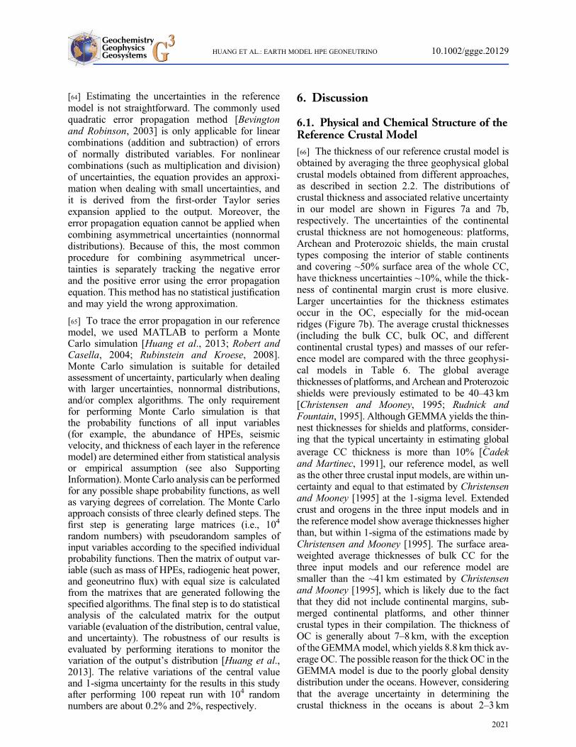
[64] Estimating the uncertainties in the referencemodel is not straightforward. The commonly usedquadratic error propagation method [Bevingtonand Robinson, 2003] is only applicable for linearcombinations (addition and subtraction) of errorsof normally distributed variables. For nonlinearcombinations (such as multiplication and division)of uncertainties, the equation provides an approxi-mation when dealing with small uncertainties, andit is derived from the first-order Taylor seriesexpansion applied to the output. Moreover, theerror propagation equation cannot be applied whencombining asymmetrical uncertainties (nonnormaldistributions). Because of this, the most commonprocedure for combining asymmetrical uncer-tainties is separately tracking the negative errorand the positive error using the error propagationequation. This method has no statistical justificationand may yield the wrong approximation.

[65] To trace the error propagation in our referencemodel, we used MATLAB to perform a MonteCarlo simulation [Huang et al., 2013; Robert andCasella, 2004; Rubinstein and Kroese, 2008].Monte Carlo simulation is suitable for detailedassessment of uncertainty, particularly when dealingwith larger uncertainties, nonnormal distributions,and/or complex algorithms. The only requirementfor performing Monte Carlo simulation is thatthe probability functions of all input variables(for example, the abundance of HPEs, seismicvelocity, and thickness of each layer in the referencemodel) are determined either from statistical analysisor empirical assumption (see also SupportingInformation).Monte Carlo analysis can be performedfor any possible shape probability functions, as wellas varying degrees of correlation. The Monte Carloapproach consists of three clearly defined steps. Thefirst step is generating large matrices (i.e., 104

random numbers) with pseudorandom samples ofinput variables according to the specified individualprobability functions. Then the matrix of output var-iable (such as mass of HPEs, radiogenic heat power,and geoneutrino flux) with equal size is calculatedfrom the matrixes that are generated following thespecified algorithms. The final step is to do statisticalanalysis of the calculated matrix for the outputvariable (evaluation of the distribution, central value,and uncertainty). The robustness of our results isevaluated by performing iterations to monitor thevariation of the output’s distribution [Huang et al.,2013]. The relative variations of the central valueand 1-sigma uncertainty for the results in this studyafter performing 100 repeat run with 104 randomnumbers are about 0.2% and 2%, respectively.

6. Discussion

6.1. Physical and Chemical Structure of theReference Crustal Model

[66] The thickness of our reference crustal model isobtained by averaging the three geophysical globalcrustal models obtained from different approaches,as described in section 2.2. The distributions ofcrustal thickness and associated relative uncertaintyin our model are shown in Figures 7a and 7b,respectively. The uncertainties of the continentalcrustal thickness are not homogeneous: platforms,Archean and Proterozoic shields, the main crustaltypes composing the interior of stable continentsand covering ~50% surface area of the whole CC,have thickness uncertainties ~10%, while the thick-ness of continental margin crust is more elusive.Larger uncertainties for the thickness estimatesoccur in the OC, especially for the mid-oceanridges (Figure 7b). The average crustal thicknesses(including the bulk CC, bulk OC, and differentcontinental crustal types) and masses of our refer-ence model are compared with the three geophysi-cal models in Table 6. The global averagethicknesses of platforms, andArchean and Proterozoicshields were previously estimated to be 40–43km[Christensen and Mooney, 1995; Rudnick andFountain, 1995]. Although GEMMA yields the thin-nest thicknesses for shields and platforms, consider-ing that the typical uncertainty in estimating globalaverage CC thickness is more than 10% [�Cadekand Martinec, 1991], our reference model, as wellas the other three crustal input models, are within un-certainty and equal to that estimated by Christensenand Mooney [1995] at the 1-sigma level. Extendedcrust and orogens in the three input models and inthe reference model show average thicknesses higherthan, but within 1-sigma of the estimations made byChristensen and Mooney [1995]. The surface area-weighted average thicknesses of bulk CC for thethree input models and our reference model aresmaller than the ~41 km estimated by Christensenand Mooney [1995], which is likely due to the factthat they did not include continental margins, sub-merged continental platforms, and other thinnercrustal types in their compilation. The thickness ofOC is generally about 7–8 km, with the exceptionof the GEMMAmodel, which yields 8.8 km thick av-erage OC. The possible reason for the thick OC in theGEMMA model is due to the poorly global densitydistribution under the oceans. However, consideringthat the average uncertainty in determining thecrustal thickness in the oceans is about 2–3 km

GeochemistryGeophysicsGeosystemsG3G3 HUANG ET AL.: EARTH MODEL HPE GEONEUTRINO 10.1002/ggge.20129

2021

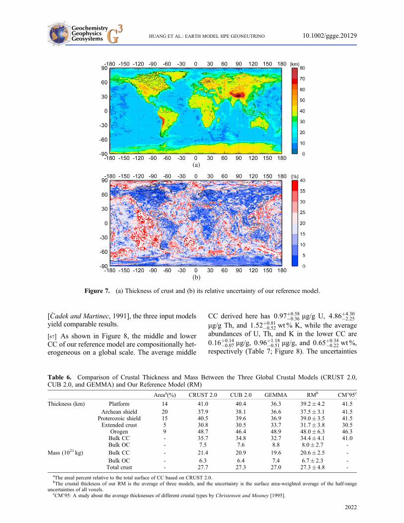
[�Cadek and Martinec, 1991], the three input modelsyield comparable results.

[67] As shown in Figure 8, the middle and lowerCC of our reference model are compositionally het-erogeneous on a global scale. The average middle

CC derived here has 0:97þ0:58�0:36 mg/g U, 4:86þ4:30

�2:25

mg/g Th, and 1:52þ0:81�0:52 wt% K, while the average

abundances of U, Th, and K in the lower CC are0:16þ0:14

�0:07 mg/g, 0:96þ1:18�0:51 mg/g, and 0:65þ0:34

�0:22 wt%,respectively (Table 7; Figure 8). The uncertainties

Figure 7. (a) Thickness of crust and (b) its relative uncertainty of our reference model.

Table 6. Comparison of Crustal Thickness and Mass Between the Three Global Crustal Models (CRUST 2.0,CUB 2.0, and GEMMA) and Our Reference Model (RM)

Areaa(%) CRUST 2.0 CUB 2.0 GEMMA RMb CM’95c

Thickness (km) Platform 14 41.0 40.4 36.3 39.2� 4.2 41.5Archean shield 20 37.9 38.1 36.6 37.5� 3.1 41.5

Proterozoic shield 15 40.5 39.6 36.9 39.0� 3.5 41.5Extended crust 5 30.8 30.5 33.7 31.7� 3.8 30.5

Orogen 9 48.7 46.4 48.9 48.0� 6.3 46.3Bulk CC - 35.7 34.8 32.7 34.4� 4.1 41.0Bulk OC - 7.5 7.6 8.8 8.0� 2.7 -

Mass (1021 kg) Bulk CC - 21.4 20.9 19.6 20.6� 2.5 -Bulk OC - 6.3 6.4 7.4 6.7� 2.3 -Total crust - 27.7 27.3 27.0 27.3� 4.8 -

aThe areal percent relative to the total surface of CC based on CRUST 2.0.bThe crustal thickness of our RM is the average of three models, and the uncertainty is the surface area-weighted average of the half-range

uncertainties of all voxels.cCM’95: A study about the average thicknesses of different crustal types by Christensen and Mooney [1995].

GeochemistryGeophysicsGeosystemsG3G3 HUANG ET AL.: EARTH MODEL HPE GEONEUTRINO 10.1002/ggge.20129

2022

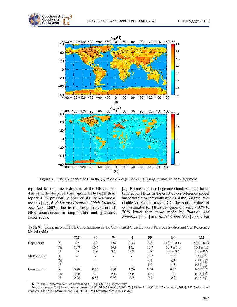
reported for our new estimates of the HPE abun-dances in the deep crust are significantly larger thanreported in previous global crustal geochemicalmodels [e.g., Rudnick and Fountain, 1995; Rudnickand Gao, 2003], due to the large dispersions ofHPE abundances in amphibolite and granulitefacies rocks.

[68] Because of these large uncertainties, all of the es-timates for HPEs in the crust of our reference modelagree with most previous studies at the 1-sigma level(Table 7). For the middle CC, the central values ofour estimates for HPEs are generally only ~10% to30% lower than those made by Rudnick andFountain [1995] and Rudnick and Gao [2003]. For

Figure 8. The abundance of U in the (a) middle and (b) lower CC using seismic velocity argument.

Table 7. Comparison of HPE Concentrations in the Continental Crust Between Previous Studies and Our ReferenceModel (RM)

TMa M W H RF RG RM

Upper crust K 2.8 2.8 2.87 2.32 2.8 2.32� 0.19 2.32� 0.19Th 10.7 10.7 10.3 10.5 10.7 10.5� 1.0 10.5� 1.0U 2.8 2.8 2.5 2.7 2.8 2.7� 0.6 2.7� 0.6

Middle crust K - - - - 1.67 1.91 1:52þ0:81�0:52

Th - - - - 6.1 6.5 4:86þ4:30�2:25

U - - - - 1.6 1.3 0:97þ0:58�0:36

Lower crust K 0.28 0.53 1.31 1.24 0.50 0.50 0:65þ0:34�0:22

Th 1.06 2.0 6.6 5.6 1.2 1.2 0:96þ1:18�0:51

U 0.28 0.53 0.93 0.7 0.2 0.2 0:16þ0:14�0:07

aK, Th, and U concentrations are listed as wt%, mg/g, and mg/g, respectively.bKeys to models: TM [Taylor and McLennan, 1995]; M [McLennan, 2001]; W [Wedepohl, 1995]; H [Hacker et al., 2011]; RF [Rudnick and

Fountain, 1995]; RG [Rudnick and Gao, 2003]; RM (Reference Model, this study).

GeochemistryGeophysicsGeosystemsG3G3 HUANG ET AL.: EARTH MODEL HPE GEONEUTRINO 10.1002/ggge.20129

2023

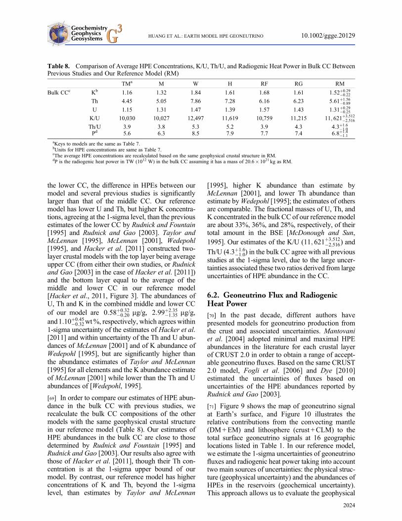
the lower CC, the difference in HPEs between ourmodel and several previous studies is significantlylarger than that of the middle CC. Our referencemodel has lower U and Th, but higher K concentra-tions, agreeing at the 1-sigma level, than the previousestimates of the lower CC by Rudnick and Fountain[1995] and Rudnick and Gao [2003]. Taylor andMcLennan [1995], McLennan [2001], Wedepohl[1995], and Hacker et al. [2011] constructed two-layer crustal models with the top layer being averageupper CC (from either their own studies, or Rudnickand Gao [2003] in the case of Hacker et al. [2011])and the bottom layer equal to the average of themiddle and lower CC in our reference model[Hacker et al., 2011, Figure 3]. The abundances ofU, Th and K in the combined middle and lower CCof our model are 0:58þ0:32

�0:20 mg/g, 2:99þ2:35�1:35 mg/g,

and1:10þ0:45�0:32wt%, respectively, which agrees within

1-sigma uncertainty of the estimates of Hacker et al.[2011] and within uncertainty of the Th and U abun-dances of McLennan [2001] and of K abundance ofWedepohl [1995], but are significantly higher thanthe abundance estimates of Taylor and McLennan[1995] for all elements and the K abundance estimateof McLennan [2001] while lower than the Th and Uabundances of [Wedepohl, 1995].

[69] In order to compare our estimates of HPE abun-dance in the bulk CC with previous studies, werecalculate the bulk CC compositions of the othermodels with the same geophysical crustal structurein our reference model (Table 8). Our estimates ofHPE abundances in the bulk CC are close to thosedetermined by Rudnick and Fountain [1995] andRudnick and Gao [2003]. Our results also agree withthose of Hacker et al. [2011], though their Th con-centration is at the 1-sigma upper bound of ourmodel. By contrast, our reference model has higherconcentrations of K and Th, beyond the 1-sigmalevel, than estimates by Taylor and McLennan

[1995], higher K abundance than estimate byMcLennan [2001], and lower Th abundance thanestimate byWedepohl [1995]; the estimates of othersare comparable. The fractional masses of U, Th, andK concentrated in the bulk CC of our referencemodelare about 33%, 36%, and 28%, respectively, of theirtotal amount in the BSE [McDonough and Sun,1995]. Our estimates of the K/U (11; 621þ3;512

�2;516) and

Th/U (4:3þ1:6�1:0) in the bulk CC agree with all previous

studies at the 1-sigma level, due to the large uncer-tainties associated these two ratios derived from largeuncertainties of HPE abundance in the CC.

6.2. Geoneutrino Flux and RadiogenicHeat Power

[70] In the past decade, different authors havepresented models for geoneutrino production fromthe crust and associated uncertainties. Mantovaniet al. [2004] adopted minimal and maximal HPEabundances in the literature for each crustal layerof CRUST 2.0 in order to obtain a range of accept-able geoneutrino fluxes. Based on the same CRUST2.0 model, Fogli et al. [2006] and Dye [2010]estimated the uncertainties of fluxes based onuncertainties of the HPE abundances reported byRudnick and Gao [2003].

[71] Figure 9 shows the map of geoneutrino signalat Earth’s surface, and Figure 10 illustrates therelative contributions from the convecting mantle(DM+EM) and lithosphere (crust +CLM) to thetotal surface geoneutrino signals at 16 geographiclocations listed in Table 1. In our reference model,we estimate the 1-sigma uncertainties of geoneutrinofluxes and radiogenic heat power taking into accounttwo main sources of uncertainties: the physical struc-ture (geophysical uncertainty) and the abundances ofHPEs in the reservoirs (geochemical uncertainty).This approach allows us to evaluate the geophysical

Table 8. Comparison of Average HPE Concentrations, K/U, Th/U, and Radiogenic Heat Power in Bulk CC BetweenPrevious Studies and Our Reference Model (RM)

TMa M W H RF RG RM

Bulk CCc Kb 1.16 1.32 1.84 1.61 1.68 1.61 1:52þ0:29�0:22

Th 4.45 5.05 7.86 7.28 6.16 6.23 5:61þ1:56�0:89

U 1.15 1.31 1.47 1.39 1.57 1.43 1:31þ0:29�0:25

K/U 10,030 10,027 12,497 11,619 10,759 11,215 11; 621þ3;512�2;516

Th/U 3.9 3.8 5.3 5.2 3.9 4.3 4:3þ1:6�1:0

Pd 5.6 6.3 8.5 7.9 7.7 7.4 6:8þ1:4�1:1

aKeys to models are the same as Table 7.bUnits for HPE concentrations are same as Table 7.cThe average HPE concentrations are recalculated based on the same geophysical crustal structure in RM.dP is the radiogenic heat power in TW (1012 W) in the bulk CC assuming it has a mass of 20.6� 1021 kg as RM.

GeochemistryGeophysicsGeosystemsG3G3 HUANG ET AL.: EARTH MODEL HPE GEONEUTRINO 10.1002/ggge.20129

2024

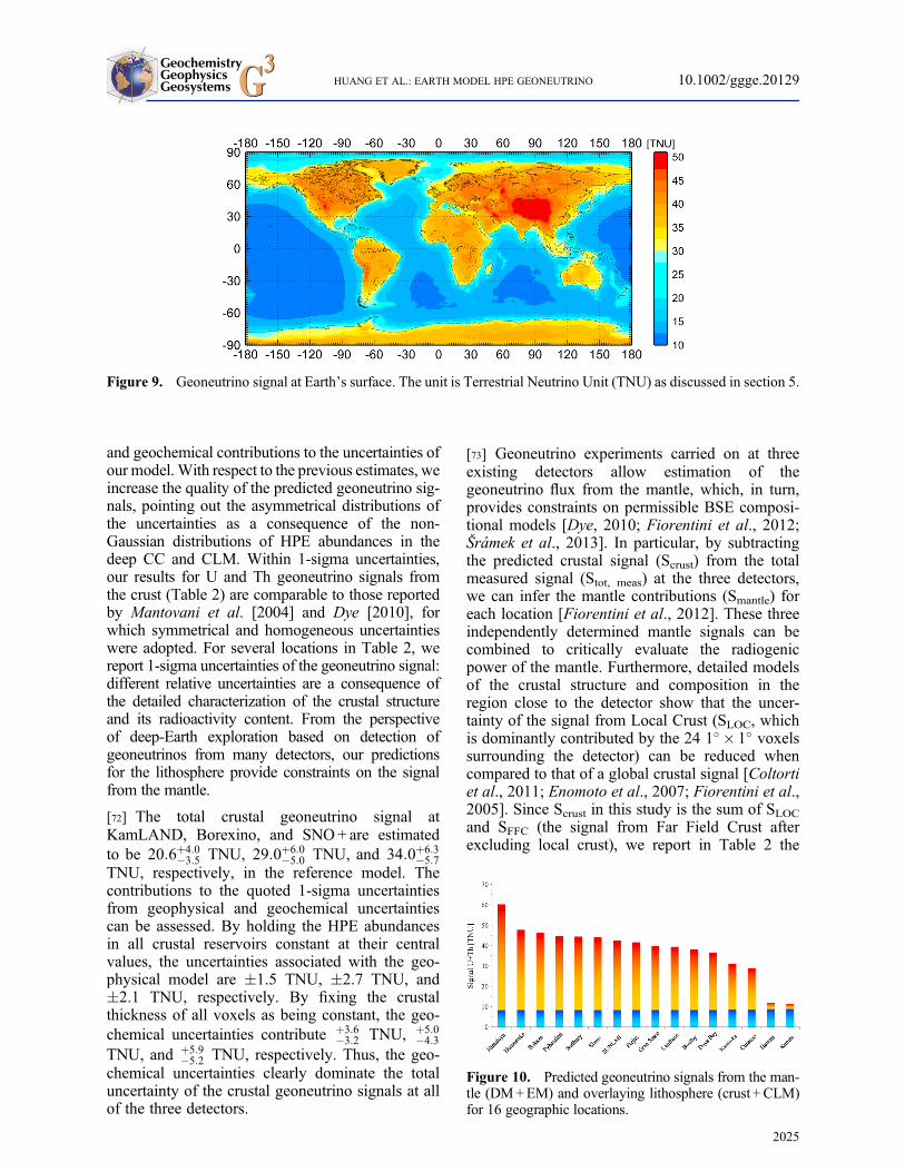
and geochemical contributions to the uncertainties ofour model. With respect to the previous estimates, weincrease the quality of the predicted geoneutrino sig-nals, pointing out the asymmetrical distributions ofthe uncertainties as a consequence of the non-Gaussian distributions of HPE abundances in thedeep CC and CLM. Within 1-sigma uncertainties,our results for U and Th geoneutrino signals fromthe crust (Table 2) are comparable to those reportedby Mantovani et al. [2004] and Dye [2010], forwhich symmetrical and homogeneous uncertaintieswere adopted. For several locations in Table 2, wereport 1-sigma uncertainties of the geoneutrino signal:different relative uncertainties are a consequence ofthe detailed characterization of the crustal structureand its radioactivity content. From the perspectiveof deep-Earth exploration based on detection ofgeoneutrinos from many detectors, our predictionsfor the lithosphere provide constraints on the signalfrom the mantle.

[72] The total crustal geoneutrino signal atKamLAND, Borexino, and SNO+ are estimatedto be 20:6þ4:0

�3:5 TNU, 29:0þ6:0�5:0 TNU, and 34:0þ6:3

�5:7TNU, respectively, in the reference model. Thecontributions to the quoted 1-sigma uncertaintiesfrom geophysical and geochemical uncertaintiescan be assessed. By holding the HPE abundancesin all crustal reservoirs constant at their centralvalues, the uncertainties associated with the geo-physical model are �1.5 TNU, �2.7 TNU, and�2.1 TNU, respectively. By fixing the crustalthickness of all voxels as being constant, the geo-chemical uncertainties contribute þ3:6

�3:2 TNU, þ5:0�4:3

TNU, and þ5:9�5:2 TNU, respectively. Thus, the geo-

chemical uncertainties clearly dominate the totaluncertainty of the crustal geoneutrino signals at allof the three detectors.

[73] Geoneutrino experiments carried on at threeexisting detectors allow estimation of thegeoneutrino flux from the mantle, which, in turn,provides constraints on permissible BSE composi-tional models [Dye, 2010; Fiorentini et al., 2012;Šrámek et al., 2013]. In particular, by subtractingthe predicted crustal signal (Scrust) from the totalmeasured signal (Stot, meas) at the three detectors,we can infer the mantle contributions (Smantle) foreach location [Fiorentini et al., 2012]. These threeindependently determined mantle signals can becombined to critically evaluate the radiogenicpower of the mantle. Furthermore, detailed modelsof the crustal structure and composition in theregion close to the detector show that the uncer-tainty of the signal from Local Crust (SLOC, whichis dominantly contributed by the 24 1� � 1� voxelssurrounding the detector) can be reduced whencompared to that of a global crustal signal [Coltortiet al., 2011; Enomoto et al., 2007; Fiorentini et al.,2005]. Since Scrust in this study is the sum of SLOCand SFFC (the signal from Far Field Crust afterexcluding local crust), we report in Table 2 the

Figure 10. Predicted geoneutrino signals from the man-tle (DM+EM) and overlaying lithosphere (crust +CLM)for 16 geographic locations.

Figure 9. Geoneutrino signal at Earth’s surface. The unit is Terrestrial Neutrino Unit (TNU) as discussed in section 5.

GeochemistryGeophysicsGeosystemsG3G3 HUANG ET AL.: EARTH MODEL HPE GEONEUTRINO 10.1002/ggge.20129

2025

geoneutrino signal SFFC (expected from the FarField Crust) on the base of our reference model.Thus, at the three existing detectors, one can sub-tract the SFFC and SLOC from the experimentallymeasured signal (Stot, meas) to define the mantlegeoneutrino signals:

Smantle ¼ Stot;meas � SFFC � SLOC (4)

[74] The CC in the reference model contributes6:8þ1:4

�1:1 TW radiogenic heat power to the total20.1 TW radiogenic power generated in the BSE,which agrees with previous estimates by Hackeret al. [2011], McLennan [2001], Rudnick andFountain [1995], and Rudnick and Gao [2003] atthe 1-sigma level, but is higher than estimate byTaylor and McLennan [1995] and lower than esti-mate by Wedepohl [1995] (Table 7). We estimatea 1-sigma uncertainty of �0.8 TW and þ1:1

�0:8 TW ofthe radiogenic heat power of the CC correspondingto geophysical and geochemical uncertainty in ourreference model, respectively.

[75] Although the mass of OC (excluding the overly-ing sediment) is poorly known, its contribution to theanticipated geoneutrino signals at the three existingdetectors is less than 0.2 TNU at the 1-sigma level.By contrast, we calculate that the CLM contributes1.6 TNU, 2.2 TNU, and 2.1 TNU to the geoneutrinosignal at KamLAND, Borexino, and SNO+, respec-tively (Table 2). The uncertainties associated with thesignal coming from this portion of lithosphere arelarge, and an increase in signal by a factor of 3 is per-mitted at the 1-sigma level. Determining the distribu-tion of U and Th in the lithospheric mantle sectionsunderlying the detectors would thus be desirable inthe future. Despite the fact that the mass of theCLM is about five times the crustal mass, it containsapproximately 10% of the total mass of HPEs in thecrust. The radiogenic heat power of CLM is0:8þ1:1

�0:6 TW: the main contribution to the uncertaintycomes from the large 1-sigma uncertainty of HPEabundances in peridotites.

7. Conclusions

[76] In this paper, we provide a reference model forthe geoneutrino flux and radiogenic heat powerfrom the main reservoirs of our planet. A particulareffort has been dedicated to estimating uncertaintiesderived from the geophysical constrains and fromthe geochemical data. We summarize here the mainresults reached in this study.

[77] 1. Three geophysical global crustal modelsbased on reflection and refraction seismic body wave(CRUST 2.0), surface wave dispersion (CUB 2.0),and gravimetric anomalies (GEMMA) are studiedwith the aim to estimate the geophysical uncertaintiesof our reference crustal model. It yields an averagecrustal thickness of 34.4� 4.1 km in the continentsand 8.0� 2.7 km in the oceans. Moreover, aglobal map of the uncertainties associated to thecrustal thickness has been produced with a grid of 1�1� voxel.[78] 2. The average continental crust derived herecontains 1:31þ0:29

�0:25 mg/g U, 5:61þ1:56�0:89 mg/g Th, and

1:52þ0:29�0:22 wt% K, has Th/U = 4:3þ1:6

�1:0 , K/U=

11; 621þ3;512�2;516 , and produces 6:8þ1:4

�1:1 TW of heat.These asymmetrical uncertainties are propagatedfrom the non-Gaussian distributions of HPEabundances in the deep continental crust andcontinental lithospheric mantle using Monte Carlosimulation.[79] 3. The radiogenic heat power in different Earthreservoirs and the geoneutrino flux at 16 geographiclocations are calculated with consideration of twomain sources of uncertainties: the physical structure(geophysical uncertainty) and the abundances ofHPEs in the reservoirs (geochemical uncertainty).Contributions from the two different sources ofuncertainty to the global uncertainties are estimatedfor the first time, and we show that the geochemicaluncertainty exerts the greatest control on the overalluncertainties.[80] 4. The geoneutrino flux from the continentallithospheric mantle (CLM) is calculated here forthe first time based on an updated xenolithic perido-tite database. The calculated geoneutrino signalfrom the CLM exceeds that from the oceanic crust(OC) at all three existing detectors.[81] 5. The combination of this global crust model,detailed local crust models, and the measured signalfor each detector provides the critical inputs neededto assess the global mantle signal and its uncertainty.Thus, the mantle signal at each detector and its uncer-tainty can be independently combined to place limits onacceptable models for the mantle’s radiogenic power.

Acknowledgments

[82] We thank Vedran Lekic for providing the data set of CUB2.0 and for insightful discussions about the seismic models. Weare grateful to Mirko Reguzzoni and Daniele Sampietro for shar-ing the GEMMA data. Discussions with MohammadBagherbandi about Moho Density Contrast model [Sjöberg andBagherbandi, 2011] helped us to understand the gravitationalanomaly model. Andrew Kerr kindly provided a geochemical

GeochemistryGeophysicsGeosystemsG3G3 HUANG ET AL.: EARTH MODEL HPE GEONEUTRINO 10.1002/ggge.20129

2026

database for basaltic oceanic plateaus. We appreciate statisticalinsights from Michael Evans, Eligio Lisi, and Gerti Xhixha.Thoughtful comments from William M. White and an anony-mous reviewer are sincerely appreciated. This study was fundedby National Science Foundation Grant EAR-1067983/1068097and partially by National Institute of Nuclear Physics (INFN).

References

Ahrens, L. H. (1954), The lognormal distribution of theelements (a fundamental law of geochemistry and its subsid-iary), Geochim. Cosmochim. Acta, 5(2), 49–73, doi:10.1016/0016-7037(54)90040-X.

Allègre, C. J., A. Hofmann, and K. O’Nions (1996), The argonconstraints on mantle structure, Geophys. Res. Lett., 23(24),3555–3557, doi:10.1029/96gl03373.

Allègre, C. J., J.-P. Poirier, E. Humler, and A. W. Hofmann(1995), The chemical composition of the Earth, Earth andPlanet. Sci. Lett., 134(3–4), 515–526, doi:10.1016/0012-821x(95)00123-t.

Alvarez Sanchez, P., et al. (2012), Measurement of CNGSmuon neutrino speed with Borexino, Phys. Lett. B, 716(3–5),401–405, doi:10.1016/j.physletb.2012.08.052.

Anderson, D. L. (2007), New Theory of the Earth, CambridgeUniversity Press, Cambridge.

Araki, T., et al. (2005), Experimental investigation of geologi-cally produced antineutrinos with KamLAND, Nature, 436(7050), 499–503, doi:10.1038/nature03980.

Arevalo, R., and W. F. McDonough (2010), Chemical varia-tions and regional diversity observed in MORB, Chem.Geol., 271(1-2), 70–85, doi:10.1016/j.chemgeo.2009.12.013.

Arevalo, R., W. F. McDonough, and M. Luong (2009), The K/U ratio of the silicate Earth: Insights into mantle composition,structure and thermal evolution, Earth Planet. Sci. Lett.,278(3-4), 361–369, doi:10.1016/j.epsl.2008.12.023.

Arevalo, R., W. F. McDonough, A. Stracke, M. Willbold, T. I.Ireland, and R. J. Walker (2013), Simplified mantle architec-ture and distribution of radiogenic power, Geochem.Geophys. Geosyst., in press.

Artemieva, I. M. (2006), Global 1� � 1� thermal model TC1 forthe continental lithosphere: Implications for lithosphere secularevolution, Tectonophysics, 416(1-4), 245–277, doi:10.1016/j.tecto.2005.11.022.

Bahcall, J. N., A. M. Serenelli, and S. Basu (2005), New solaropacities, abundances, helioseismology, and neutrino fluxes,The Astrophys. J. Lett., 621(1), L85, doi:10.1086/428929.

Bassin, C., G. Laske, and T. G. Masters (2000), The currentlimits of resolution for surface wave tomography in NorthAmerica, EOS Trans.

Behn, M. D., and P. B. Kelemen (2003), Relationship betweenseismic P-wave velocity and the composition of anhydrousigneous and meta-igneous rocks, Geochem. Geophys.Geosyst., 4(5), 1041, doi:10.1029/2002gc000393.

Bellini, G., et al. (2010), Observation of geo-neutrinos,Physics Letters B, 687(4–5), 299–304, doi:10.1016/j.physletb.2010.03.051.

Bellini, G., et al. (2013), Measurement of geo-neutrinos from1353 days of Borexino, arXiv:1303.2571.

Bemporad, C., G. Gratta, and P. Vogel (2002), Reactor-basedneutrino oscillation experiments, Rev. Mod. Phys., 74(2),297–328, doi:10.1103/RevModPhys.74.297.

Bevington, P. R., and D. K. Robinson (2003), Data Reductionand Error Analysis for the Physical Sciences, McGraw-Hill,Boston, 3rd edition.

Birch, F. (1960), The velocity of compressional waves in rocksto 10-kilobars .1, J. Geophys. Res., 65(4), 1083–1102,doi:10.1029/JZ065i004p01083.

Boyet, M., and R. W. Carlson (2005), 142Nd evidence for early(>4.53Ga) global differentiation of the silicate Earth,Science, 309(5734), 576–581, doi:10.1126/science.1113634.

Buklerskii, A. V., A. M. Kart, B. S. Klyachko, V. K. Kravchuk,V. K. Milyukov, I. V. Melezhnikov, A. V. Myasnikov, V. V.Nesterov, and V. N. Rudenko (1995), Baksen laser interferom-eter, Meas. Tech., 38(10), 1995.

�Cadek, O., and Z. Martinec (1991), Spherical harmonic expan-sion of the Earth’s crustal thickness up to degree and order30, Stud. Geophys. Geod., 35(3), 151–165, doi:10.1007/bf01614063.

Chen, M. C. (2006), Geo-neutrinos in SNO+, Earth, Moon,Planets, 99(1-4), 221–228, doi:10.1007/s11038-006-9116-4.

Christensen, N. I., and W. D. Mooney (1995), Seismic velocitystructure and composition of the continental crust: A globalview, J. Geophys. Res.-Solid Earth, 100(B6), 9761–9788,doi:10.1029/95jb00259.

Coltorti, M., et al. (2011), U and Th content in the CentralApennines continental crust: A contribution to the determina-tion of the geo-neutrinos flux at LNGS,Geochim. Cosmochim.Acta, 75(9), 2271–2294, doi:10.1016/j.gca.2011.01.024.

Conrad, C. P., and C. Lithgow-Bertelloni (2006), Influenceof continental roots and asthenosphere on plate-mantle cou-pling, Geophys. Res. Lett., 33(5), L05312, doi: 10.1029/2005gl025621.

De Meijer, R. J., F. D. Smit, F. D. Brooks, R. W. Fearick, H. J.Wörtche, and F.Mantovani (2006), Towards Earth antineutrinotomography (EARTH), Earth, Moon, and Planets, 99(1-4),193–206, doi:10.1007/s11038-006-9104-8.

Dye, S. T. (2010), Geo-neutrinos and silicate earth enrichmentof U and Th, Earth Planet. Sci. Lett., 297(1-2), 1–9,doi:10.1016/j.epsl.2010.06.012.

Dye, S. T. (2012), Geoneutrinos and the radioactive power of theEarth, Reviews of Geophysics, 50(3), doi:10.1029/2012rg000400.

Dziewonski, A. M., and D. L. Anderson (1981), Preliminaryreference Earth model, Phys. Earth Planet. Inter., 25, 297–356,doi:10.1016/0031-9201(81)90046-7.

Enomoto, S., E. Ohtani, K. Inoue, and A. Suzuki (2007),Neutrino geophysics with KamLAND and future prospects,Earth Planet. Sci. Lett., 258(1-2), 147–159, doi:10.1016/j.epsl.2007.03.038.

Fiorentini, G., M. Lissia, and F. Mantovani (2007), Geo-neutri-nos and Earth’s interior, Phys. Rep., 453(5-6), 117–172,doi:10.1016/j.physrep.2007.09.001.

Fiorentini, G., M. Lissia, F. Mantovani, and B. Ricci(2005), KamLAND results and the radiogenic terrestrialheat, Phys. Lett. B, 629(2–4), 77–82, doi:10.1016/j.physletb.2005.09.067.

Fiorentini, G., G. Fogli, E. Lisi, F. Mantovani, and A. Rotunno(2012), Mantle geoneutrinos in KamLAND and Borexino,Phys. Rev. D, 86(3), doi:10.1103/PhysRevD.86.033004.

Fiorentini, G., A. Ianni, G. Korga, M. Lissia, F. Mantovani, L.Miramonti, L. Oberauer, M. Obolensky, O. Smirnov, and Y.Suvorov (2010), Nuclear physics for geo-neutrino studies,Phys. Rev. C, 81(3), doi:10.1103/PhysRevC.81.034602.

Fogli, G. L., E. Lisi, A. Palazzo, and A. M. Rotunno (2006),Geo-neutrinos: A systematic approach to uncertainties andcorrelations, Earth, Moon, and Planets, 99(1-4), 111–130,doi:10.1007/s11038-006-9107-5.

Fogli, G. L., E. Lisi, A. Marrone, A. Palazzo, and A. M.Rotunno (2011), Evidence of θ13> 0 from global neutrino dataanalysis, Phys. Rev. D, 84(5), 053007, doi:10.1103/PhysRevD.84.053007.

GeochemistryGeophysicsGeosystemsG3G3 HUANG ET AL.: EARTH MODEL HPE GEONEUTRINO 10.1002/ggge.20129

2027

Gando, A., et al. (2011), Partial radiogenic heat model forEarth revealed by geoneutrino measurements, Nat. Geosci.,4(9), 647–651, doi:10.1038/ngeo1205.

Gando, A., et al. (2013), Reactor on-off antineutrino measure-ment with KamLAND, arXiv1303.4667.

Goldschmidt, V. M. (1933), Grundlagen der quantitativenGeochemie, Fortschr. Mienral. Kirst. Petrogr., 17, 112.

Gung, Y., M. Panning, and B. Romanowicz (2003),Global anisotropy and the thickness of continents, Nature,422(6933), 707–711, doi:10.1038/nature01559.

Hacker, B. R., P. B. Kelemen, and M. D. Behn (2011), Differ-entiation of the continental crust by relamination, EarthPlanet. Sci. Lett., 307(3–4), 501–516, doi:10.1016/j.epsl.2011.05.024.

Hart, S. R., and A. Zindler (1986), In search of a bulk-Earthcomposition, Chem. Geol., 57(3–4), 247–267, doi:10.1016/0009-2541(86)90053-7.

Hofmann, A. W., andW.M.White (1983), Ba, Rb, and Cs in theEarth’s mantle, Zeitschrift Naturforschung Teil A, 38, 256–266.

Holbrook, W. S., W. D. Mooney, and N. I. Christensen (1992),The seismic velocity structure of the deep continental crust,in Lower Continental Crust, edited by D. M. Fountain, R.Arculus and R. Kay, pp. 1–43, Elsevier, Amsterdam.

Huang, Y., W. F. McDonough, and F. Mantovani (2013),Propagation of uncertainties in geochemistry by Monte Carlosimulation, Chem. Geol., under review.

Jaupart, C., and J. C. Mareschal (1999), The thermal structureand thickness of continental roots, Lithos, 48(1–4), 93–114,doi:10.1016/s0024-4937(99)00023-7.

Jaupart, C., J. C. Mareschal, L. Guillou-Frottier, and A. Davaille(1998), Heat flow and thickness of the lithosphere in theCanadian Shield, J. Geophys. Res., 103(B7), 15,269–215,286.

Javoy, M., et al. (2010), The chemical composition of theEarth: Enstatite chondrite models, Earth and Planet. Sci. Lett.,293(3-4), 259–268, doi:10.1016/j.epsl.2010.02.033.

Jordan, T. H. (1975), The continental tectosphere, Rev.Geophys., 13(3), 1–12, doi:10.1029/RG013i003p00001.

Kobayashi, M., and Y. Fukao (1991), The Earth as an antineu-trino star, Geophys. Res. Lett., 18(4), 633–636, doi:10.1029/91gl00800.

Korenaga, J. (2008), Urey ratio and the structure and evolutionof Earth’s mantle, Rev. Geophys., 46(2), doi:10.1029/2007rg000241.

Kramers, J. D., and I. N. Tolstikhin (1997), Two terrestrial leadisotope paradoxes, forward transport modelling, core forma-tion and the history of the continental crust, Chem. Geol.,139(1–4), 75–110, doi:10.1016/s0009-2541(97)00027-2.

Labrosse, S., and C. Jaupart (2007), Thermal evolution of theEarth: Secular changes and fluctuations of plate characteristics,Earth and Planet. Sci. Lett., 260(3-4), 465–481, doi:10.1016/j.epsl.2007.05.046.

Labrosse, S., J. W. Hernlund, and N. Coltice (2007), A crystal-lizing dense magma ocean at the base of the Earth/’s mantle,Nature, 450(7171), 866–869, doi:10.1038/nature06355.

Laske, G., and T. G. Masters (1997), A global digital map ofsediment thickness, EOS Trans. AGU, 78F483.

Laske, G., T. G. Masters, and C. Reif, (2001), CRUST 2.0: Anew global crustal model at 2 x 2 degrees, http://igppweb.ucsd.edu/~gabi/crust2.htm

Le Bas, M. J., and A. L. Streckeisen (1991), The IUGS system-atics of igneous rocks, J. Geol. Soc., 148(5), 825–833,doi:10.1144/gsjgs.148.5.0825.

Lee, C.-T. A., P. Luffi, T. Hoink, J. Li, R. Dasgupta, andJ. Hernlund (2010), Upside-down differentiation and generationof a ’primordial’ lower mantle, Nature, 463(7283), 930–933,doi:10.1038/nature08824.

Lewis, J. S. (1971), Consequences of the presence of sulfurin the core of the earth, Earth and Planet. Sci. Lett., 11(1–5),130–134, doi:10.1016/0012-821x(71)90154-3.

Lyubetskaya, T., and J. Korenaga (2007a), Chemical composi-tion of Earth’s primitive mantle and its variance: 2. Implica-tions for global geodynamics, J. Geophys. Res., 112(B3),B03212, doi: 10.1029/2005jb004224.

Lyubetskaya, T., and J. Korenaga (2007b), Chemical composi-tion of Earth’s primitive mantle and its variance: 1. Methodand results, J. Geophys. Res., 112(B3), B03211, doi:10.1029/2005jb004223.

Mantovani, F., L. Carmignani, G. Fiorentini, and M. Lissia(2004), Antineutrinos from Earth: A reference model andits uncertainties, Phys. Rev. D, 69(1), doi:10.1103/PhysRevD.69.013001.

McDonough,W. F. (1990), Constraints on the composition of thecontinental lithospheric mantle, Earth and Planet. Sci. Lett.,101(1), 1–18, doi:10.1016/0012-821x(90)90119-i.

McDonough, W. F. (2003), Compositional model for the Earth’score, in TheMantle andCore, Vol. 2 Treatise onGeochemistry,edited by R. W. Carlson, Elsevier, Oxford, pp. 547–568.

McDonough, W. F., and S.-S. Sun (1995), The compositionof the Earth, Chem. Geol., 120, 223–253, doi:10.1016/0009-2541(94)00140-4.

McLennan, S. M. (2001), Relationships between the trace ele-ment composition of sedimentary rocks and upper continen-tal crust, Geochem. Geophys. Geosyst., 2(4), doi:10.1029/2000gc000109.

Mooney, W. D., G. Laske, and T. G. Masters (1998), CRUST5.1: A global crustal model at 5o� 5o, J. Geophys. Res.,103(B1), 727–747, doi:10.1029/97JB02122.

Murakami, M., Y. Ohishi, N. Hirao, and K. Hirose (2012), Aperovskitic lower mantle inferred from high-pressure, high-temperature sound velocity data, Nature, 485(7396), 90–94,doi:10.1038/nature11004.

Murrell, M. T., and D. S. Burnett (1986), Partitioning of K, U,and Th between sulfide and silicate liquids: Implicationsfor radioactive heating of planetary cores, J. Geophys. Res.,91(B8), 8126–8136, doi:10.1029/JB091iB08p08126.

Murthy, V. R.,W. vanWestrenen, and Y. Fei (2003), Experimen-tal evidence that potassium is a substantial radioactive heatsource in planetary cores, Nature, 423(6936), 163–165,doi:10.1038/nature01560.

Nataf, H.-C., and Y. Richard (1996), 3SMAC: An a prioritomographic model of the upper mantle based on geophysicalmodeling, Phys. Earth Planet. Inter., 95, 101–122,doi:10.1016/0031-9201(95)03105-7.

Negretti, M., M. Reguzzoni, and D. Sampietro (2012), Aweb processing service for GOCE data exploitation, in FirstInternational GOCE Solid Earth Workshop, Enschede, TheNetherlands.

O’Neill, H. S. C., and H. Palme (2008), Collisional erosion andthe non-chondritic composition of the terrestrial planets,Philosophical Transactions of the Royal Society A: Mathe-matical, Physical and Eng. Sci., 366(1883), 4205–4238,doi:10.1098/rsta.2008.0111.

Pail, R., et al. (2011), First GOCE gravity field models derivedby three different approaches, J. Geod., 85(11), 819–843,doi:10.1007/s00190-011-0467-X.

Palme, H., and H. S. C. O’Neill (2003), Cosmochemicalestimates of mantle composition, in The Mantle and Core,Vol. 2 Treatise of Geochemistry, edited by R. W. Carlson,pp. 1–38, Elsevier, Oxford.

Parsons, T., N. I. Christensen, and H. G. Wilshire (1995),Velocities of southern Basin and Range xenoliths: Insightson the nature of lower crustal reflectivity and composition,

GeochemistryGeophysicsGeosystemsG3G3 HUANG ET AL.: EARTH MODEL HPE GEONEUTRINO 10.1002/ggge.20129

2028

Geology, 23(2), 129–132, doi:10.1130/0091-7613(1995)023< 0129:vosbar> 2.3.co;2.

Pasyanos, M. E. (2010), Lithospheric thickness modeledfrom long-period surface wave dispersion, Tectonophysics,481(1-4), 38–50, doi:10.1016/j.tecto.2009.02.023.

Plank, T. (2013), The chemical composition of subductingsediments, in Treatise of Geochemistry, 2nd ed., Elsevier,Oxford.

Pollack, H. N., and D. S. Chapman (1977), On the regionalvariation of heat flow, geotherms, and lithospheric thickness,Tectonophysics, 38(3–4), 279–296, doi:10.1016/0040-1951(77)90215-3.

Porter, K. A., and W. M. White (2009), Deep mantle subduc-tion flux, Geochem. Geophys. Geosyst., 10(12), Q12016,doi: 10.1029/2009gc002656.

Reguzzoni, M., and N. Tselfes (2009), Optimal multi-stepcollocation: application to the space-wise approach forGOCE data analysis, J. Geod., 83(1), 13–29, doi:10.1007/s00190-008-0225-X.

Reguzzoni, M., and D. Sampietro (2012), Moho estimationusing GOCE data: A numerical simulation, in Geodesy forPlanet Earth, edited by S. Kenyon, M. C. Pacino and U.Marti, pp. 205–214, Springer, Berlin, Heidelberg.

Robert, C. P., and G. Casella (2004), Monte Carlo StatisticalMethods, 2nd ed., Springer, New York.

Rubinstein, R. Y., and D. P. Kroese (2008), Simulation and theMonte Carlo Method, Student Solution Manual, 2nd ed.,John Wiley & Sons. Inc., Hoboken, New Jersey.

Rudnick, R. L., and D. M. Fountain (1995), Nature and composi-tion of the continental crust: A lower crustal perspective, Rev.Geophys., 33(3), 267–309, doi:10.1029/95rg01302.

Rudnick, R. L., and I. Jackson (1995), Measured and calculatedelastic wave speeds in partially equilibrated mafic granulite xe-noliths: Implications fro the properties of an underplated lowercontinental crust, J. Geophys. Res.-Solid Earth, 100(B6),10211–10218, doi:10.1029/94jb03261.

Rudnick, R. L., and A. A. Nyblade (1999), The compositionand thickness of Archean continental roots: constraints fromxenolith thermobarometry, in Mantle Petrology: FieldObservations and High-Pressure Experimentation: A Tributeto Francis R. (Joe) Boyd, edited by Y. Fei, C. M. Bertka andB. O. Mysen, pp. 3–12, Geochemical Society Special Publi-cation 6, St. Louis, MO.

Rudnick, R. L., and S. Gao (2003), Composition of the conti-nental crust, in The Crust, Vol. 3 Treatise on Geochemistry,edited by R. L. Rudnick, Elsevier, Oxford, pp. 1–64.

Rudnick, R. L., W. F. McDonough, and R. J. O’Connell (1998),Thermal structure, thickness and composition of continentallithosphere, Chem. Geol., 145, 395–411, doi:10.1016/S0009-2541(97)00151-4.

Shapiro, N. M., and M. H. Ritzwoller (2002), Monte-Carloinversion for a global shear-velocity model of the crust andupper mantle, Geophys. J. Int., 151, 88–105, doi:10.1046/j.1365-246X.2002.01742.X.

Sjöberg, L. E., and M. Bagherbandi (2011), A method ofestimating the Moho density contrast with a tentativeapplication of EGM08 and CRUST2.0, Acta Geophys.,59(3), 502–525, doi:10.2478/s11600-011-0004-6.

Sobolev, S., and A. Babeyko (1994), Modeling of mineralogicalcomposition, density and elastic wave velocities inanhydrous magmatic rocks, Surv Geophys., 15(5), 515–544,doi:10.1007/bf00690173.

Šrámek, O.,W. F.McDonough, E. S. Kite, V. Lekić, S. T. Dye, andS. Zhong (2013), Geophysical and geochemical constraints ongeoneutrino fluxes from Earth’s mantle, Earth and Planet. Sci.Lett., 361, 356–366, doi:10.1016/j.epsl.2012.11.001.

Staudigel, H. (2003), Hydrotherml alteration processes in theoceanic crust, in The Crust, vol. 3 Treatise on Geochemistry,edited by R. L. Rudnick, Elsevier, Oxford, pp. 511–535 .

Taylor, S. R., and S. M. McLennan (1995), The geochemicalevolution of the continental crust, Rev. Geophys., 33(2),241–265, doi:10.1029/95rg00262.

Tenzer, R., K. Hamayun, and P. Vajda (2009), Global maps of theCRUST 2.0 crustal components stripped gravity disturbances,J. Geophys. Res., 114(B5), B05408, doi: 10.1029/2008jb006016.

Tolich, N., Y. D. Chan, C. A. Currat, B. K. Fujikawa, R.Henning, K. T. Lesko, A. W. P. Poon, M. P. Decowski, J.Wang, and K. Tolich (2006), A geoneutrino experiment atHomestake, Earth, Moon, and Planets, 99(1-4), 229–240,doi:10.1007/s11038-006-9112-8.

Turcotte, D. L., and G. Schubert (2002), Geodynamics, Applica-tions of Continuum Physics to Geological Problems, 2nd ed.,Cambridge University Press, Cambridge, UK.

Turcotte, D. L., D. Paul, andW.M.White (2001), Thorium-uraniumsystematics require layered mantle convection, J. Geophys.Res., 106(B3), 4265–4276, doi:10.1029/2000jb900409.

van der Hilst, R. D., S. Widiyantoro, and E. R. Engdahl (1997),Evidence for deep mantle circulation from global tomogra-phy, Nature, 386(6625), 578–584, doi:10.1038/386578a0.

Wang, Y. F. (2011), Daya Bay experiment and its future.Rep., Venice.

Warren, P. H. (2011), Stable-isotopic anomalies and the accre-tionary assemblage of the Earth and Mars: A subordinaterole for carbonaceous chondrites, Earth Planet. Sci. Lett.,311(1–2), 93–100, doi:10.1016/j.epsl.2011.08.047.

Wedepohl, K. H. (1995), The composition of the continentalcrust, Geochim. Cosmochim. Acta, 59(7), 1217–1232,doi:10.1016/0016-7037(95)00038-2.

White, W. M., and E. M. Klein (2013), The oceanic crust, inTreatise of Geochemistry, 2nd edition, edited.

Wurm, M., et al. (2012), The next-generation liquid-scintillatorneutrino observatory LENA,Astropart. Phys., 35(11), 685–732,doi:10.1016/j.astropartphys.2012.02.011.

Yoder, C. F. (1995), Astrometric and geodetic properties of Earthand the solar system, in Global Earth Physics: A Handbook ofPhysical Constants, edited by T. J. Ahrens, pp. 1–31, AGUreference shelf Series No. 1, American Geophysical Union,Washington, D.C.

GeochemistryGeophysicsGeosystemsG3G3 HUANG ET AL.: EARTH MODEL HPE GEONEUTRINO 10.1002/ggge.20129

2029