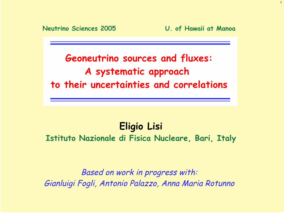
Geoneutrino sources and fluxes:A systematic approach

to their uncertainties and correlations

Eligio LisiIstituto Nazionale di Fisica Nucleare, Bari, Italy

Neutrino Sciences 2005 U. of Hawaii at Manoa

1

Based on work in progress with: Gianluigi Fogli, Antonio Palazzo, Anna Maria Rotunno

2

Congratulations to the KamLAND collaboration!

3

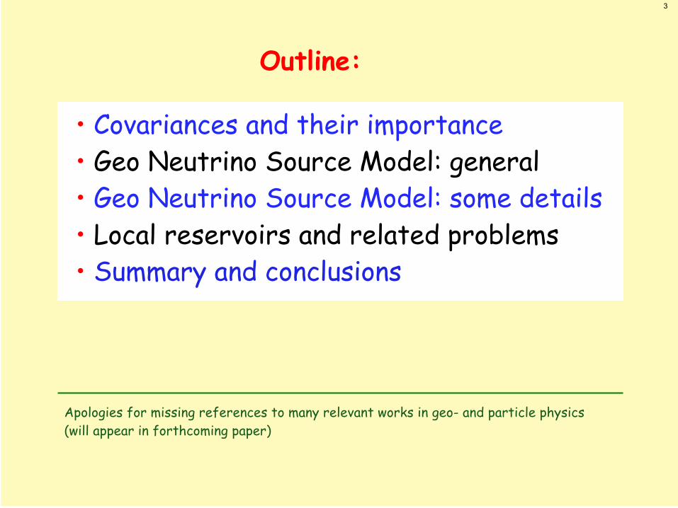
• Covariances and their importance • Geo Neutrino Source Model: general• Geo Neutrino Source Model: some details• Local reservoirs and related problems• Summary and conclusions

Apologies for missing references to many relevant works in geo- and particle physics(will appear in forthcoming paper)

Outline:

4

Covariances and their importance

5

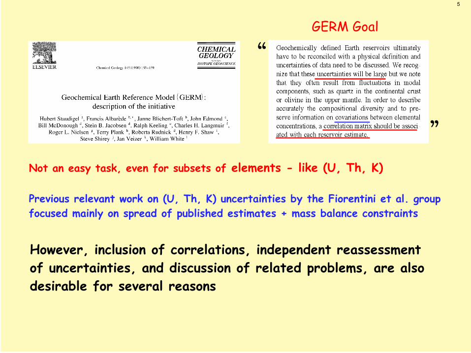
Not an easy task, even for subsets of elements - like (U, Th, K)

Previous relevant work on (U, Th, K) uncertainties by the Fiorentini et al. group focused mainly on spread of published estimates + mass balance constraints

However, inclusion of correlations, independent reassessment of uncertainties, and discussion of related problems, are alsodesirable for several reasons

“

”

GERM Goal

6

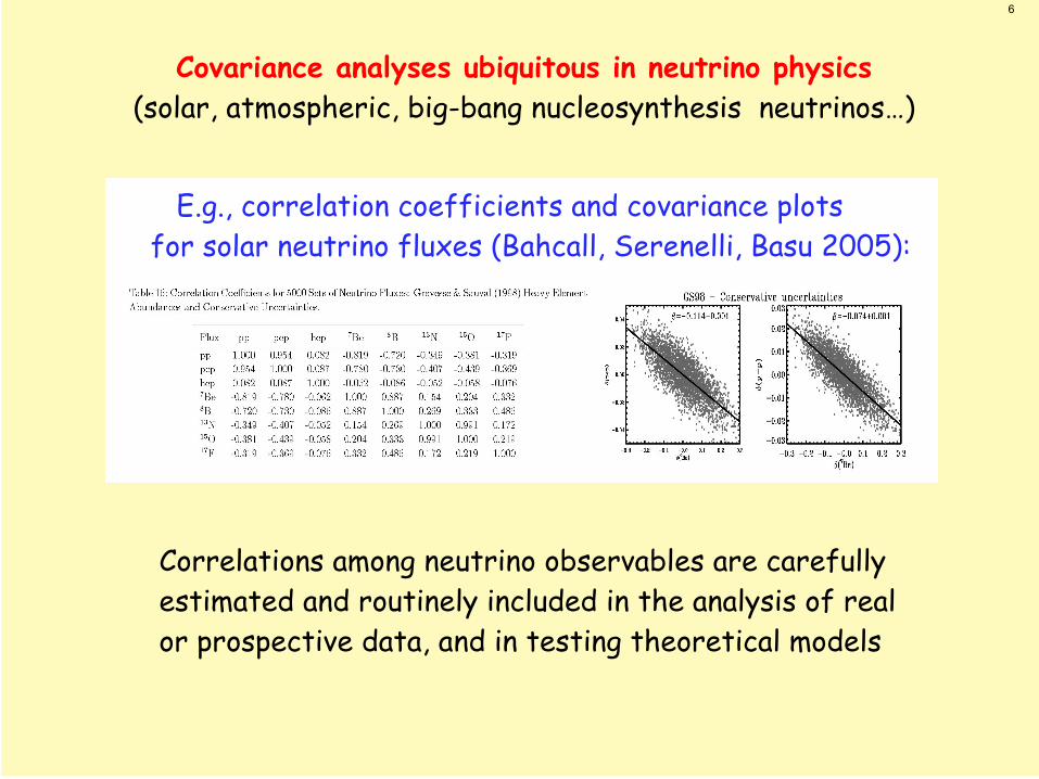
Covariance analyses ubiquitous in neutrino physics(solar, atmospheric, big-bang nucleosynthesis neutrinos…)

E.g., correlation coefficients and covariance plotsfor solar neutrino fluxes (Bahcall, Serenelli, Basu 2005):

Correlations among neutrino observables are carefullyestimated and routinely included in the analysis of realor prospective data, and in testing theoretical models

7

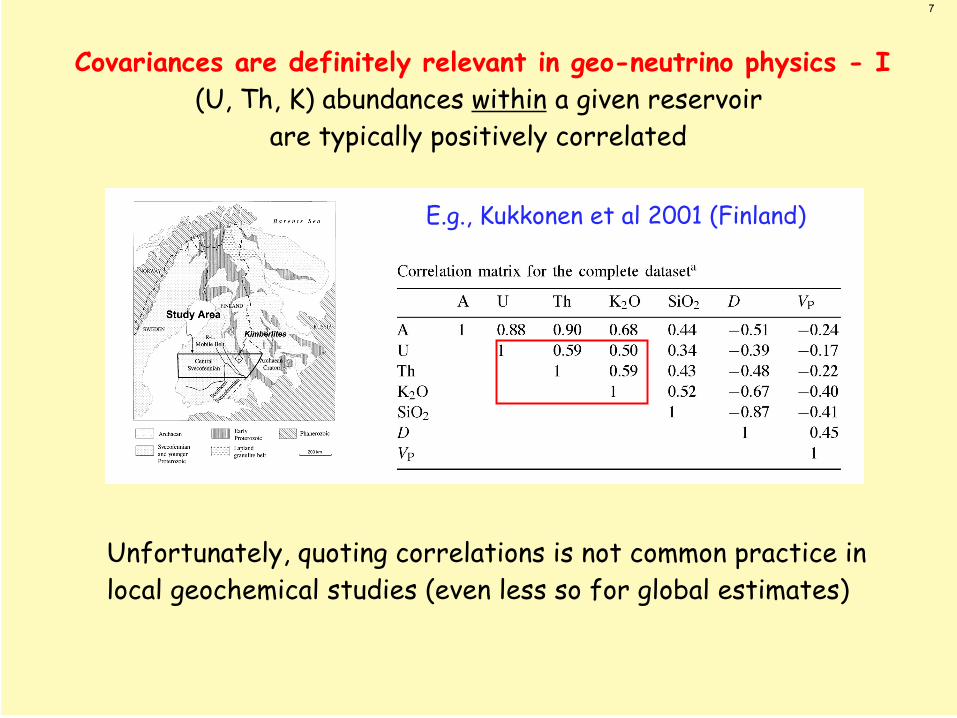
Covariances are definitely relevant in geo-neutrino physics - I(U, Th, K) abundances within a given reservoir

are typically positively correlated

Unfortunately, quoting correlations is not common practice inlocal geochemical studies (even less so for global estimates)

E.g., Kukkonen et al 2001 (Finland)

8

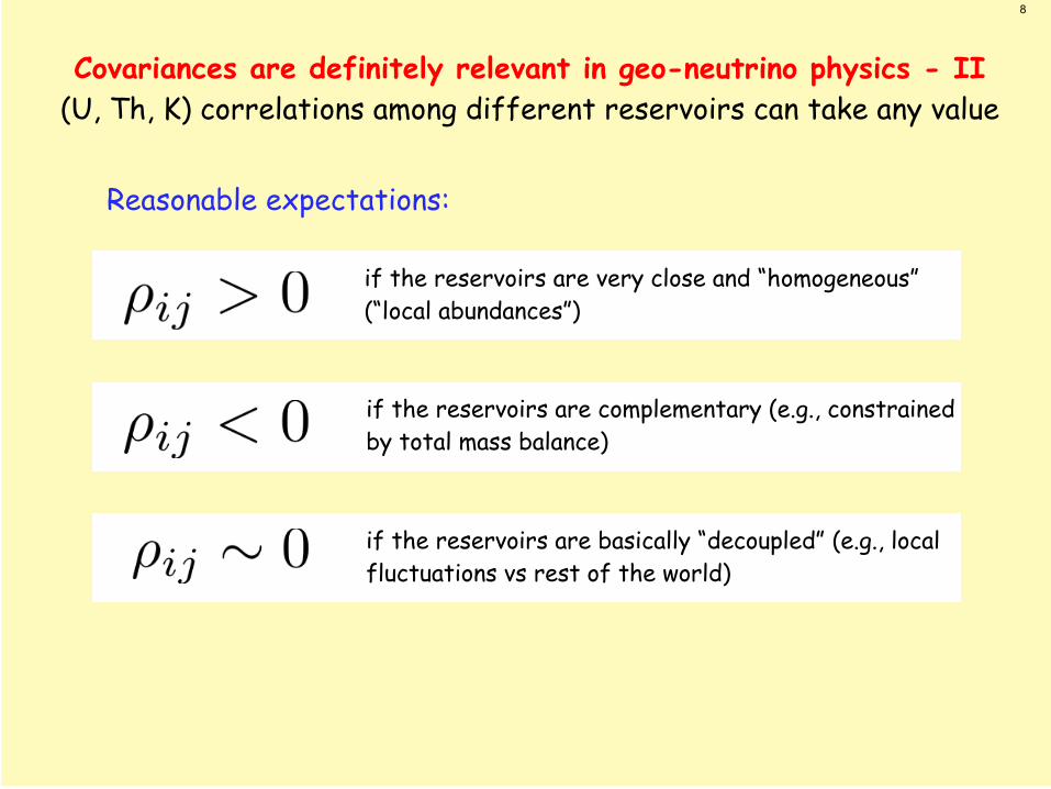
Covariances are definitely relevant in geo-neutrino physics - II(U, Th, K) correlations among different reservoirs can take any value

if the reservoirs are complementary (e.g., constrainedby total mass balance)

if the reservoirs are very close and “homogeneous”(“local abundances”)

if the reservoirs are basically “decoupled” (e.g., localfluctuations vs rest of the world)

Reasonable expectations:

9

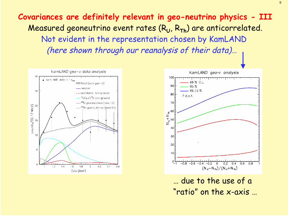
Covariances are definitely relevant in geo-neutrino physics - IIIMeasured geoneutrino event rates (RU, RTh) are anticorrelated.

Not evident in the representation chosen by KamLAND (here shown through our reanalysis of their data)…

… due to the use of a “ratio” on the x-axis …

10

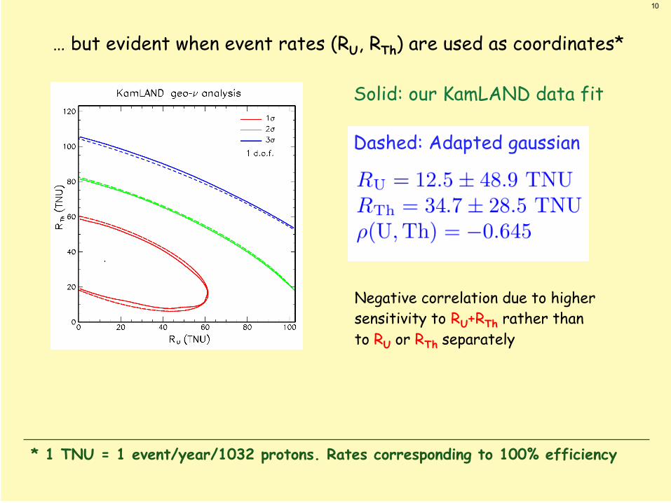
… but evident when event rates (RU, RTh) are used as coordinates*

* 1 TNU = 1 event/year/1032 protons. Rates corresponding to 100% efficiency

Solid: our KamLAND data fit

Negative correlation due to highersensitivity to RU+RTh rather thanto RU or RTh separately

Dashed: Adapted gaussian

11

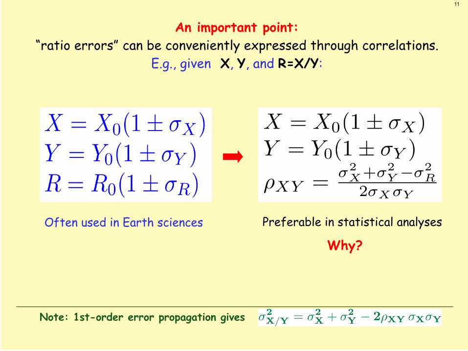
An important point:“ratio errors” can be conveniently expressed through correlations.

E.g., given X, Y, and R=X/Y:

Often used in Earth sciences Preferable in statistical analyses

Why?

Note: 1st-order error propagation gives

12

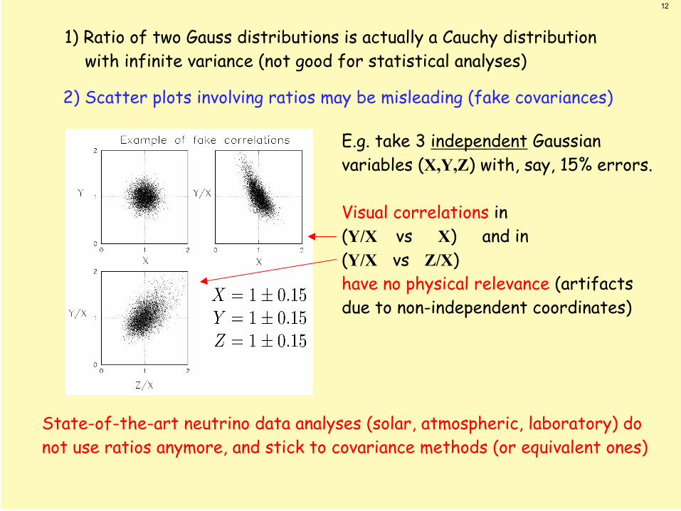
1) Ratio of two Gauss distributions is actually a Cauchy distribution with infinite variance (not good for statistical analyses)

2) Scatter plots involving ratios may be misleading (fake covariances)

E.g. take 3 independent Gaussianvariables (X,Y,Z) with, say, 15% errors.

Visual correlations in(Y/X vs X) and in(Y/X vs Z/X)have no physical relevance (artifactsdue to non-independent coordinates)

State-of-the-art neutrino data analyses (solar, atmospheric, laboratory) donot use ratios anymore, and stick to covariance methods (or equivalent ones)

13

GNSM: general aspects

14

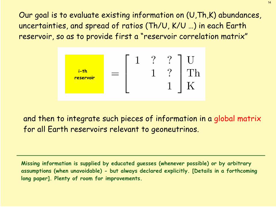
Our goal is to evaluate existing information on (U,Th,K) abundances,uncertainties, and spread of ratios (Th/U, K/U …) in each Earth reservoir, so as to provide first a “reservoir correlation matrix”

i-th reservoir

and then to integrate such pieces of information in a global matrix for all Earth reservoirs relevant to geoneutrinos.

Missing information is supplied by educated guesses (whenever possible) or by arbitrary assumptions (when unavoidable) - but always declared explicitly. [Details in a forthcoming long paper]. Plenty of room for improvements.

15

Assumed structure of the total correlation matrix of abundances:(local=close to given detectors; global=rest of the world)

GlobalReservoirs

(OC, CC, UM, LM)

Local 1

Local 2

Local 3

Basically we assume that “local” abundance fluctuations are decoupled fromglobal abundance uncertainties (this must be true after a certain distance).

Of course, definition of what is a “local” reservoir is not innocent.

OC = Oceanic CrustCC = Continental CrustUM = Upper MantleLM = Lower mantle

(Core excluded for simplicity)

16

CC

CC

UM

OC

LM

LM

UM

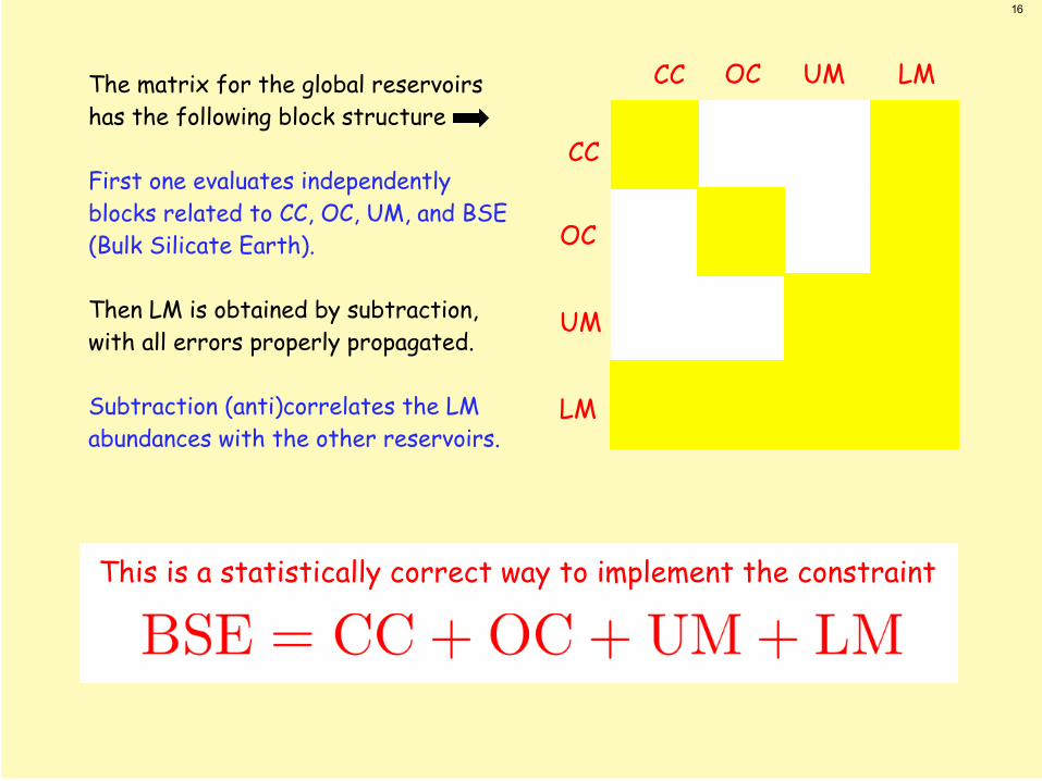
OCThe matrix for the global reservoirshas the following block structure

First one evaluates independently blocks related to CC, OC, UM, and BSE (Bulk Silicate Earth).

Then LM is obtained by subtraction, with all errors properly propagated.

Subtraction (anti)correlates the LMabundances with the other reservoirs.

This is a statistically correct way to implement the constraint

17

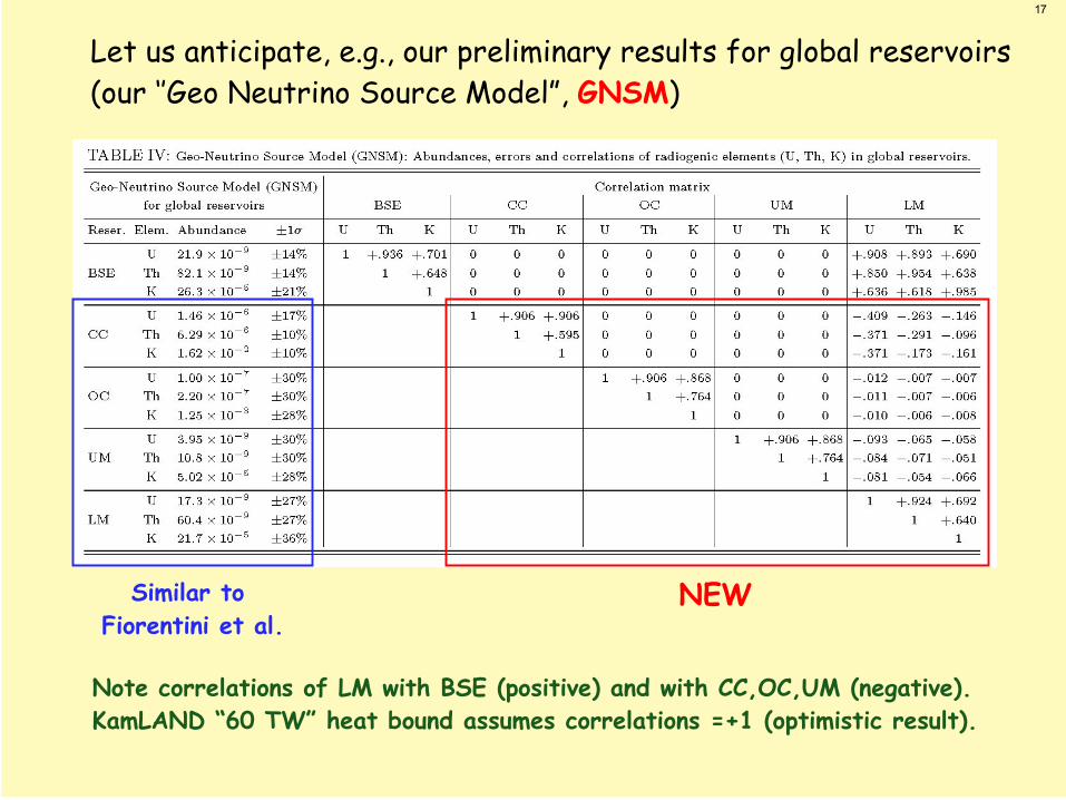
Let us anticipate, e.g., our preliminary results for global reservoirs(our ‘’Geo Neutrino Source Model”, GNSM)

Similar to Fiorentini et al.

NEW

Note correlations of LM with BSE (positive) and with CC,OC,UM (negative).KamLAND “60 TW” heat bound assumes correlations =+1 (optimistic result).

18

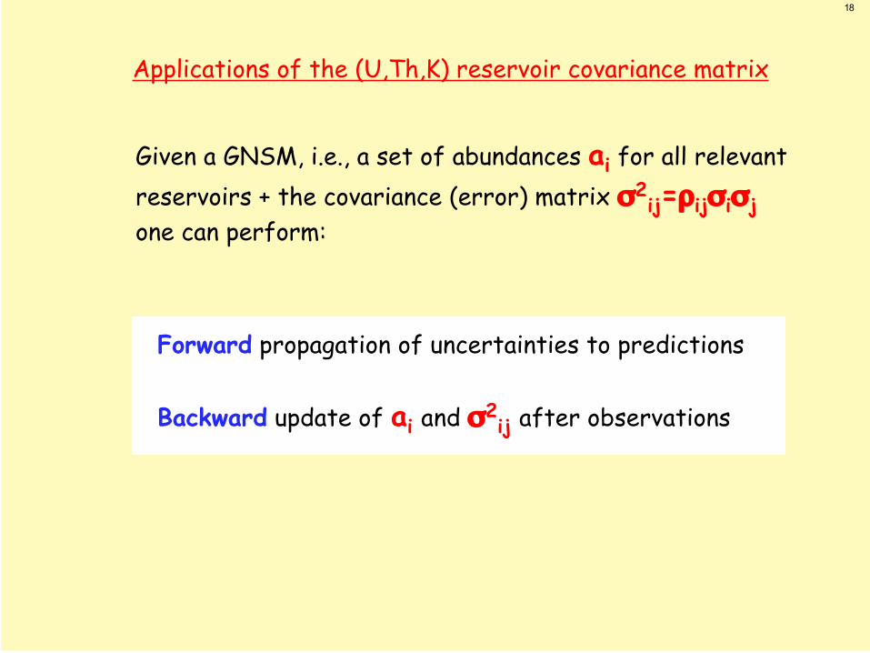
Applications of the (U,Th,K) reservoir covariance matrix

Given a GNSM, i.e., a set of abundances ai for all relevantreservoirs + the covariance (error) matrix σ2

ij=ρijσiσjone can perform:

Forward propagation of uncertainties to predictions

Backward update of ai and σ2ij after observations

19

ForwardSeveral quantities of interest (total elemental mass, radiogenic heat, geoneutrino fluxes and event rates) are linear combinations of the (U,Th,K) abundances with

known coefficients:

Their “theoretical” errors and correlations (induced by uncertainties ofthe GNSM) are then easily computed as

20

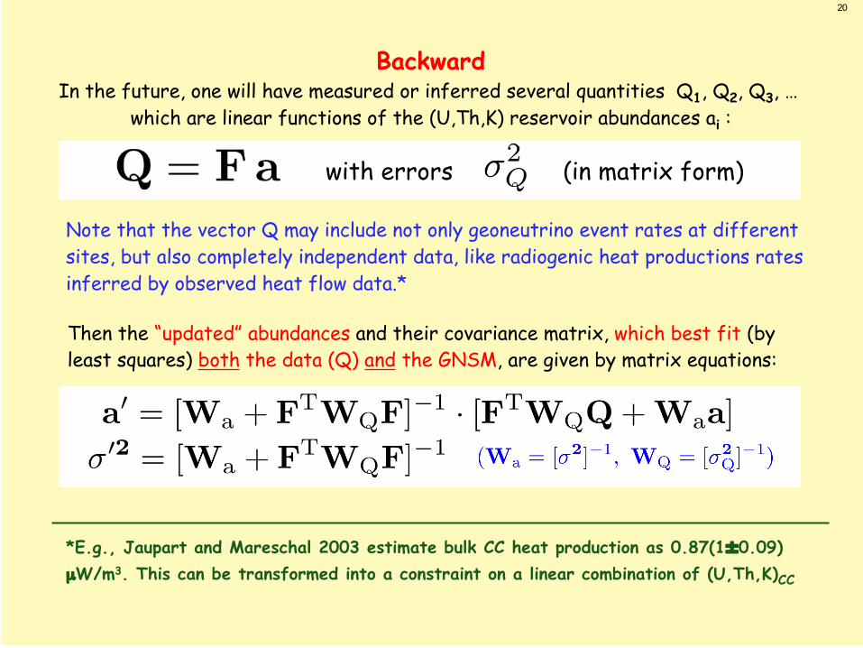
BackwardIn the future, one will have measured or inferred several quantities Q1, Q2, Q3, …

which are linear functions of the (U,Th,K) reservoir abundances ai :

Note that the vector Q may include not only geoneutrino event rates at differentsites, but also completely independent data, like radiogenic heat productions ratesinferred by observed heat flow data.*

with errors (in matrix form)

*E.g., Jaupart and Mareschal 2003 estimate bulk CC heat production as 0.87(1±0.09)µW/m3. This can be transformed into a constraint on a linear combination of (U,Th,K)CC

Then the “updated” abundances and their covariance matrix, which best fit (byleast squares) both the data (Q) and the GNSM, are given by matrix equations:

21

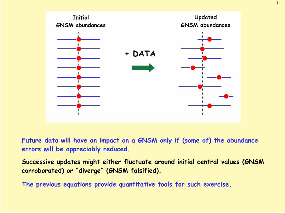
InitialGNSM abundances

UpdatedGNSM abundances

+ DATA

Future data will have an impact on a GNSM only if (some of) the abundanceerrors will be appreciably reduced.

Successive updates might either fluctuate around initial central values (GNSMcorroborated) or “diverge” (GNSM falsified).

The previous equations provide quantitative tools for such exercise.

22

GNSM construction: some details

23

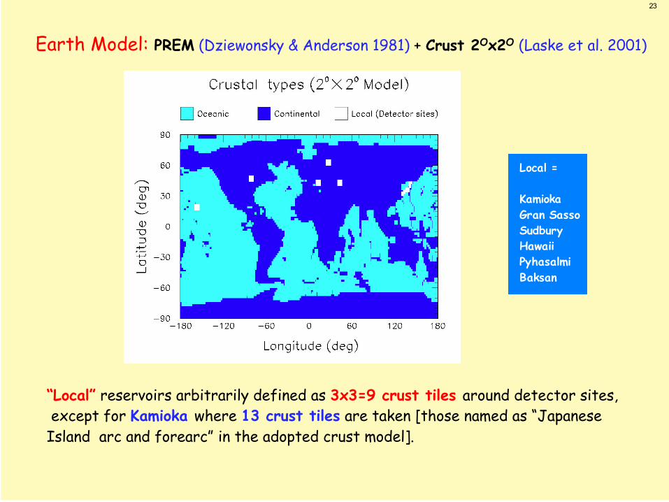
Earth Model: PREM (Dziewonsky & Anderson 1981) + Crust 2Ox2O (Laske et al. 2001)

Local =

KamiokaGran SassoSudburyHawaiiPyhasalmiBaksan

“Local” reservoirs arbitrarily defined as 3x3=9 crust tiles around detector sites, except for Kamioka where 13 crust tiles are taken [those named as “JapaneseIsland arc and forearc” in the adopted crust model].

24

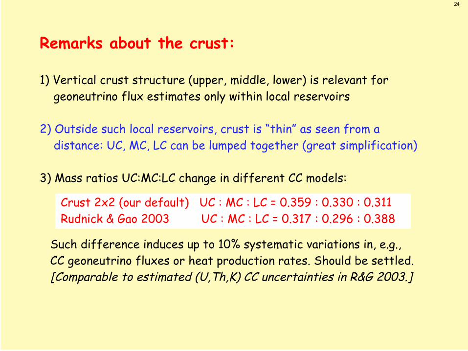
Remarks about the crust:

1) Vertical crust structure (upper, middle, lower) is relevant for geoneutrino flux estimates only within local reservoirs

2) Outside such local reservoirs, crust is “thin” as seen from a distance: UC, MC, LC can be lumped together (great simplification)

3) Mass ratios UC:MC:LC change in different CC models:

Crust 2x2 (our default) UC : MC : LC = 0.359 : 0.330 : 0.311 Rudnick & Gao 2003 UC : MC : LC = 0.317 : 0.296 : 0.388

Such difference induces up to 10% systematic variations in, e.g., CC geoneutrino fluxes or heat production rates. Should be settled. [Comparable to estimated (U,Th,K) CC uncertainties in R&G 2003.]

25

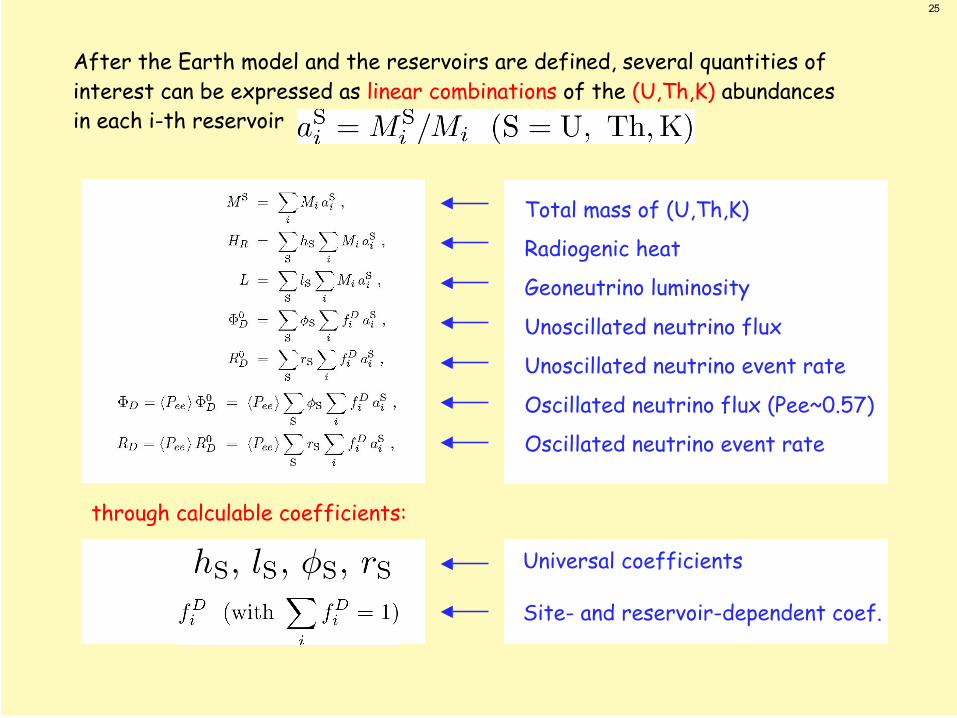
After the Earth model and the reservoirs are defined, several quantities of interest can be expressed as linear combinations of the (U,Th,K) abundances in each i-th reservoir

through calculable coefficients:

Total mass of (U,Th,K)

Radiogenic heat

Geoneutrino luminosity

Unoscillated neutrino flux

Unoscillated neutrino event rate

Oscillated neutrino flux (Pee~0.57)

Oscillated neutrino event rate

Universal coefficients

Site- and reservoir-dependent coef.

26

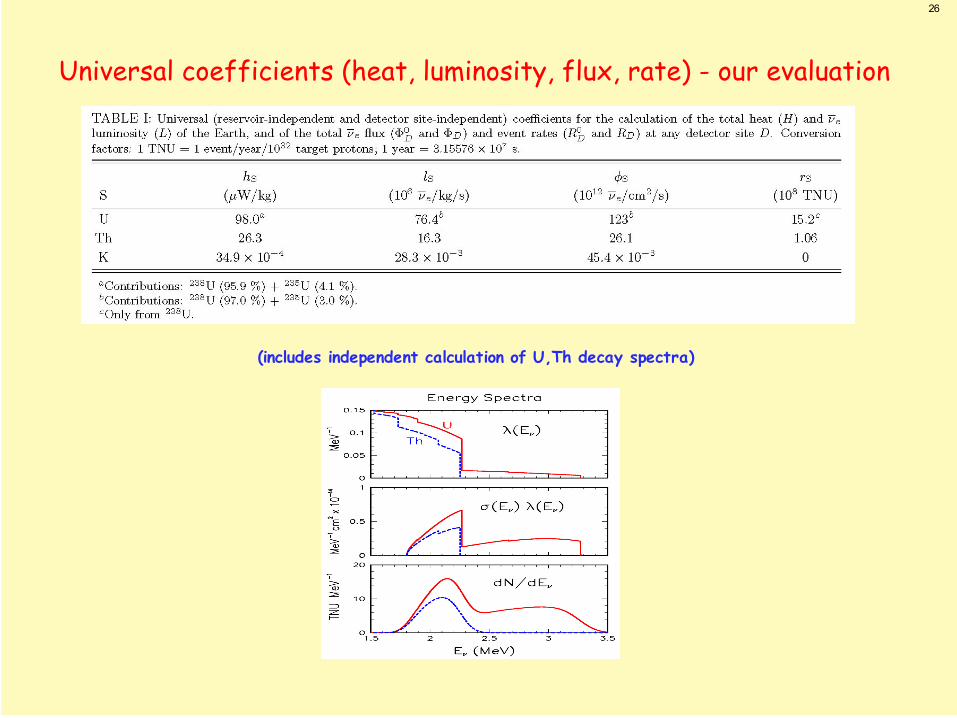
Universal coefficients (heat, luminosity, flux, rate) - our evaluation

(includes independent calculation of U,Th decay spectra)

27

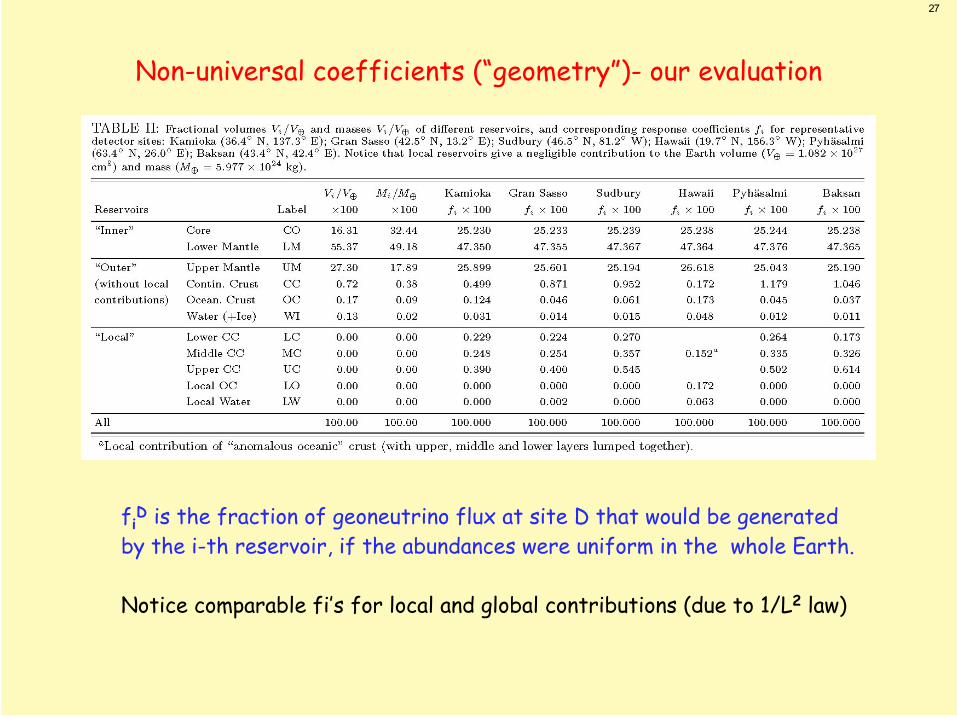
Non-universal coefficients (“geometry”)- our evaluation

fiD is the fraction of geoneutrino flux at site D that would be generated

by the i-th reservoir, if the abundances were uniform in the whole Earth.

Notice comparable fi’s for local and global contributions (due to 1/L2 law)

28

Such coefficients have relatively minor uncertainties, whichcan be neglected at this stage.

[Some systematic deviations among independent published values for universal coefficients may be attributed, e.g., to old decay orcross-section data, or to neglect of U-235]

The main task is thus reduced, as anticipated, to assess reasonable (U,Th,K) abundances (central values, errors, and covariances fromratios) based on existing geo-literature and databases.

Not a straightforward task, in general...

Famous quotes:

29

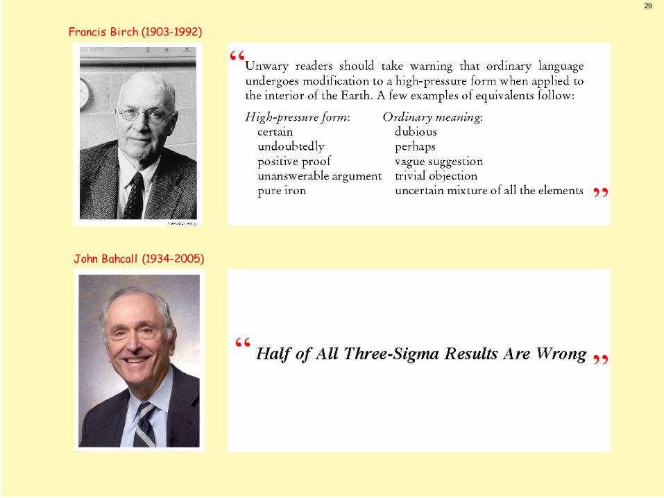
Francis Birch (1903-1992)

John Bahcall (1934-2005)

“

”

“ ”

30

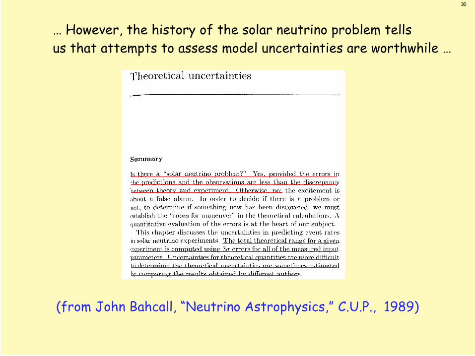
… However, the history of the solar neutrino problem tellsus that attempts to assess model uncertainties are worthwhile …

(from John Bahcall, “Neutrino Astrophysics,” C.U.P., 1989)

31

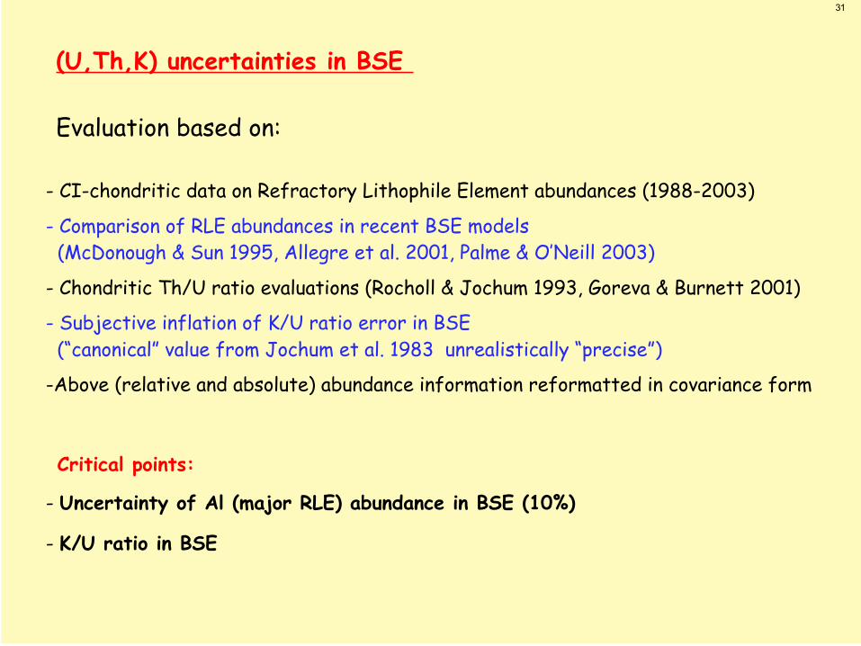
(U,Th,K) uncertainties in BSE

Evaluation based on:

- CI-chondritic data on Refractory Lithophile Element abundances (1988-2003)

- Comparison of RLE abundances in recent BSE models (McDonough & Sun 1995, Allegre et al. 2001, Palme & O’Neill 2003)

- Chondritic Th/U ratio evaluations (Rocholl & Jochum 1993, Goreva & Burnett 2001)

- Subjective inflation of K/U ratio error in BSE (“canonical” value from Jochum et al. 1983 unrealistically “precise”)

-Above (relative and absolute) abundance information reformatted in covariance form

Critical points:

- Uncertainty of Al (major RLE) abundance in BSE (10%)

- K/U ratio in BSE

32

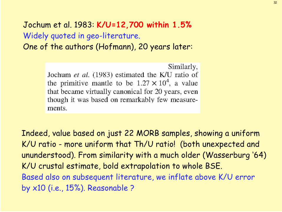
Jochum et al. 1983: K/U=12,700 within 1.5%Widely quoted in geo-literature.One of the authors (Hofmann), 20 years later:

Indeed, value based on just 22 MORB samples, showing a uniformK/U ratio - more uniform that Th/U ratio! (both unexpected and ununderstood). From similarity with a much older (Wasserburg ‘64) K/U crustal estimate, bold extrapolation to whole BSE. Based also on subsequent literature, we inflate above K/U error by x10 (i.e., 15%). Reasonable ?

33

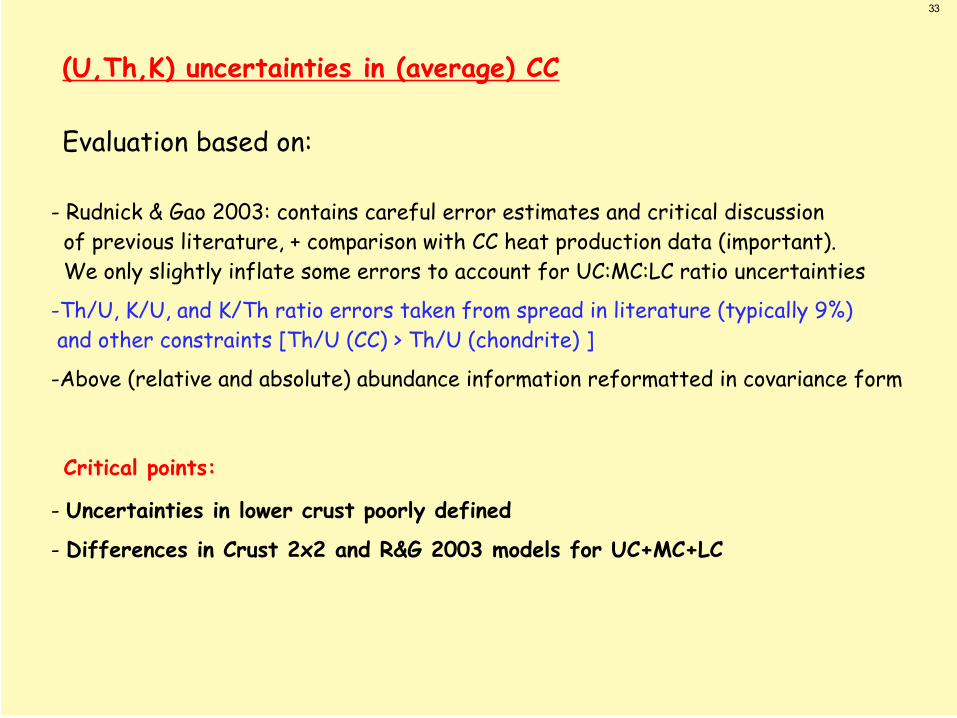
(U,Th,K) uncertainties in (average) CC

Evaluation based on:

- Rudnick & Gao 2003: contains careful error estimates and critical discussion of previous literature, + comparison with CC heat production data (important). We only slightly inflate some errors to account for UC:MC:LC ratio uncertainties

-Th/U, K/U, and K/Th ratio errors taken from spread in literature (typically 9%) and other constraints [Th/U (CC) > Th/U (chondrite) ]

-Above (relative and absolute) abundance information reformatted in covariance form

Critical points:

- Uncertainties in lower crust poorly defined

- Differences in Crust 2x2 and R&G 2003 models for UC+MC+LC

34

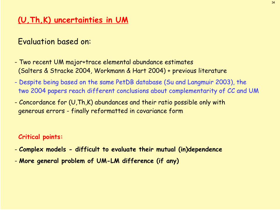
(U,Th,K) uncertainties in UM

Evaluation based on:

- Two recent UM major+trace elemental abundance estimates (Salters & Stracke 2004, Workmann & Hart 2004) + previous literature

- Despite being based on the same PetDB database (Su and Langmuir 2003), the two 2004 papers reach different conclusions about complementarity of CC and UM

- Concordance for (U,Th,K) abundances and their ratio possible only with generous errors - finally reformatted in covariance form

Critical points:

- Complex models - difficult to evaluate their mutual (in)dependence

- More general problem of UM-LM difference (if any)

35

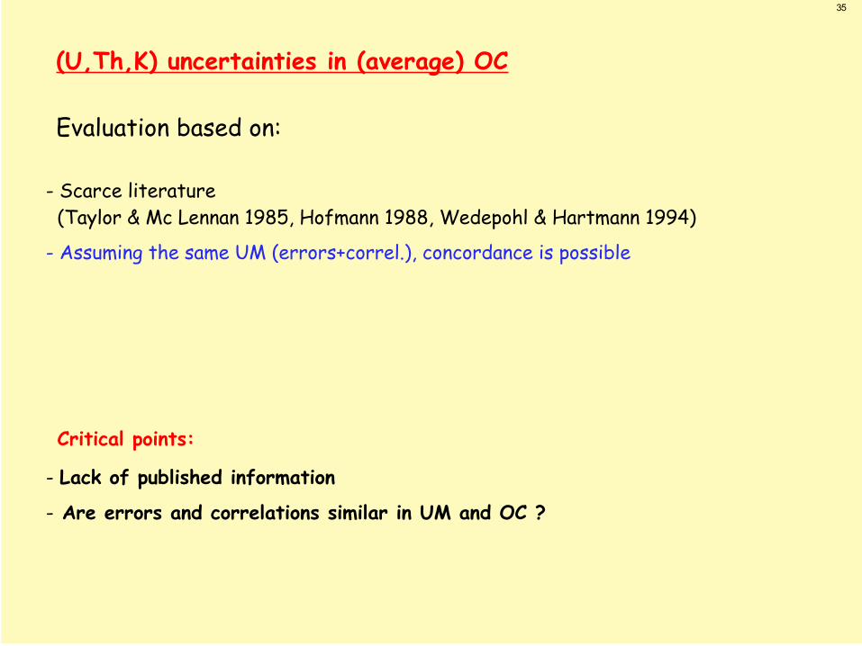
(U,Th,K) uncertainties in (average) OC

Evaluation based on:

- Scarce literature (Taylor & Mc Lennan 1985, Hofmann 1988, Wedepohl & Hartmann 1994)

- Assuming the same UM (errors+correl.), concordance is possible

Critical points:

- Lack of published information

- Are errors and correlations similar in UM and OC ?

36

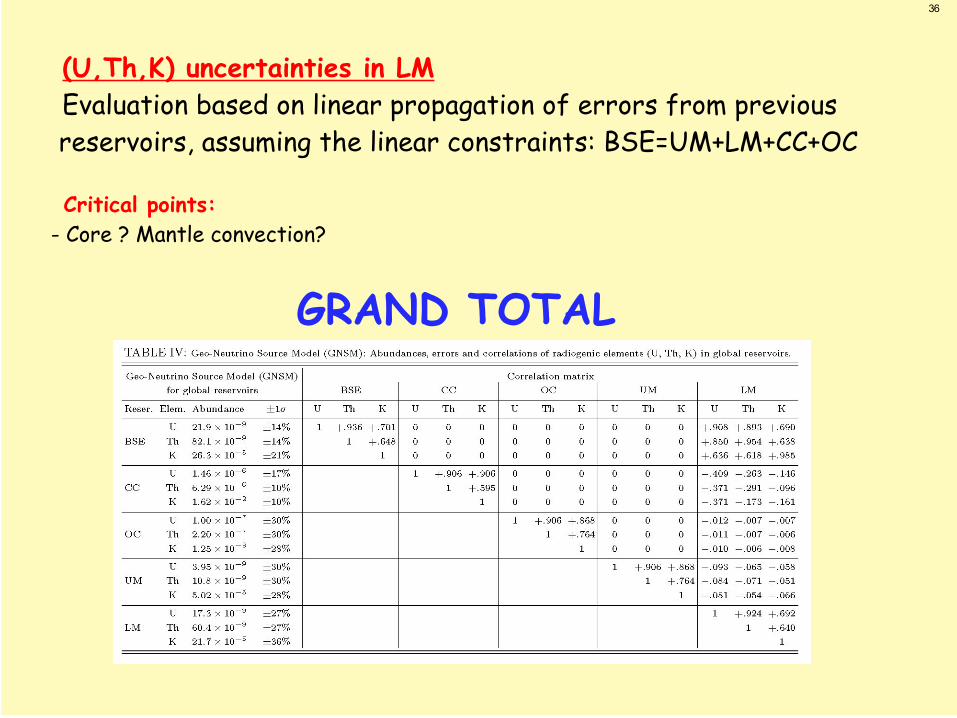
(U,Th,K) uncertainties in LM Evaluation based on linear propagation of errors from previous reservoirs, assuming the linear constraints: BSE=UM+LM+CC+OC Critical points:- Core ? Mantle convection?

GRAND TOTAL

37

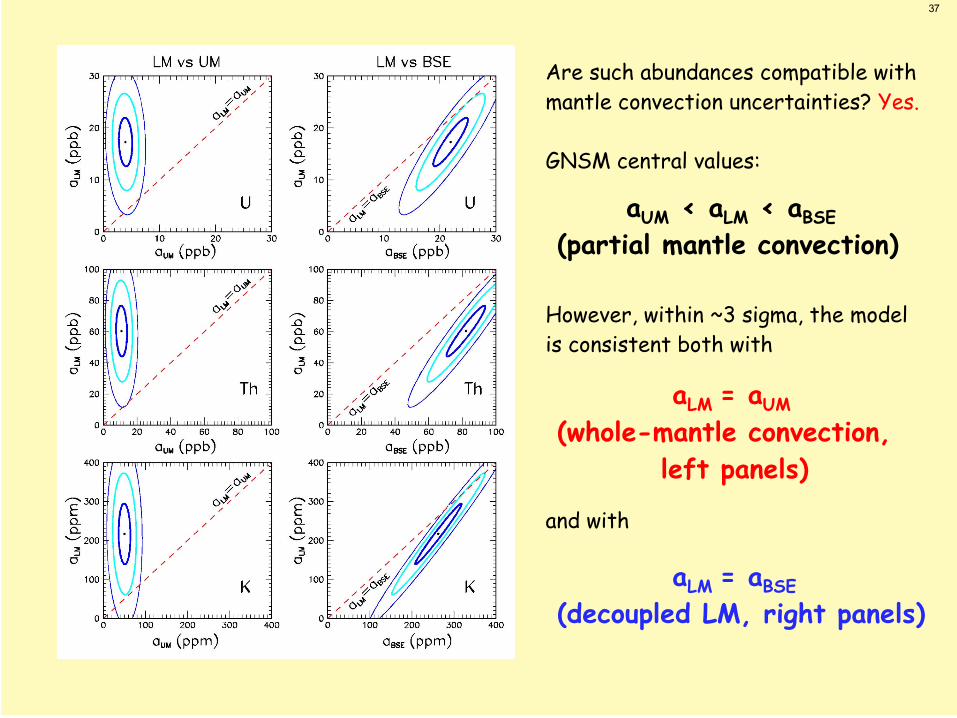
Are such abundances compatible withmantle convection uncertainties? Yes.

GNSM central values:

aUM < aLM < aBSE

(partial mantle convection)

However, within ~3 sigma, the modelis consistent both with

aLM = aUM

(whole-mantle convection, left panels)

and with

aLM = aBSE

(decoupled LM, right panels)

38

Local reservoirs and related problems

39

The characterization of local crust reservoirs (which give a large- but not necessarily interesting - contribution to the geoneutrino signal) is not easy. Problems:

2x2 crust resolution is poorHorizontal distribution of (U,Th,K) often not well knownVertical distribution of (U,Th,K) largely unknownElemental ratios (e.g., Th/U) may locally be anomalous …

However, at least some of these problems can be solvedby merging existing information on:

3D local models of the crust (and mantle)(Un)published rock sample databasesSurface heat flow dataBorehole data …

Interdisciplinary approach + long-term work required

40

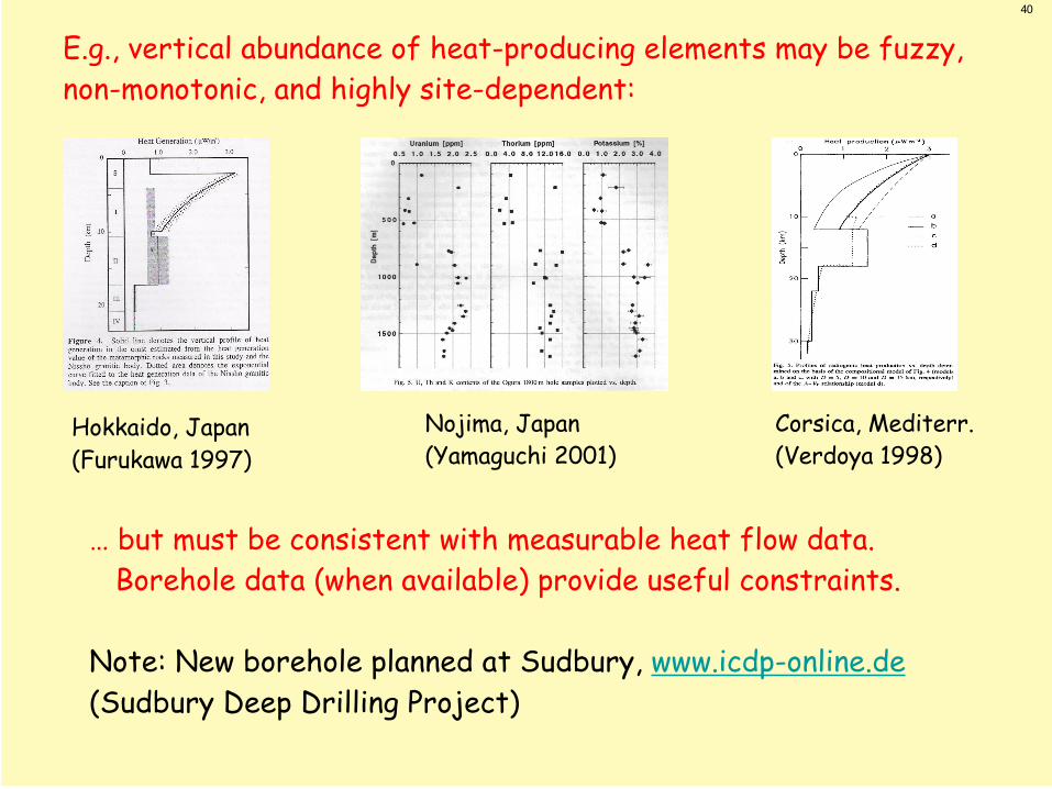
E.g., vertical abundance of heat-producing elements may be fuzzy,non-monotonic, and highly site-dependent:

Hokkaido, Japan(Furukawa 1997)

Nojima, Japan(Yamaguchi 2001)

Corsica, Mediterr.(Verdoya 1998)

… but must be consistent with measurable heat flow data. Borehole data (when available) provide useful constraints.

Note: New borehole planned at Sudbury, www.icdp-online.de(Sudbury Deep Drilling Project)

41

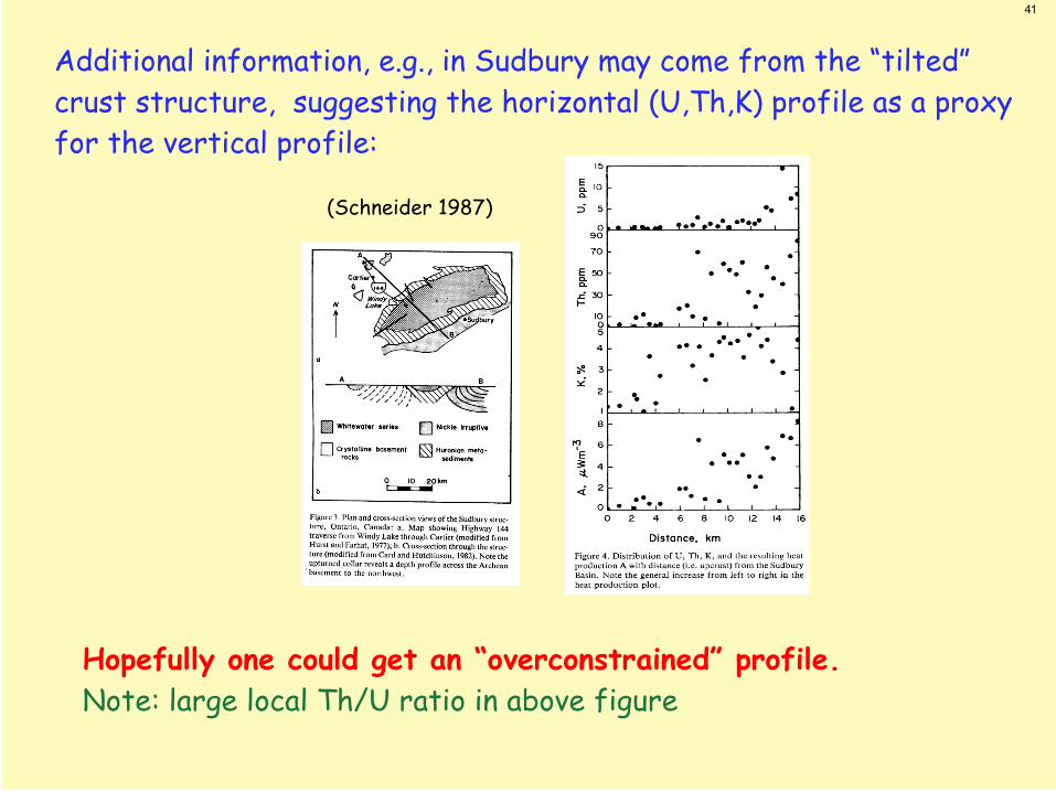
Additional information, e.g., in Sudbury may come from the “tilted” crust structure, suggesting the horizontal (U,Th,K) profile as a proxy for the vertical profile:

(Schneider 1987)

Hopefully one could get an “overconstrained” profile. Note: large local Th/U ratio in above figure

42

Inter-disciplinary work desirable to assess local uncertainties.By merging available (+new?) local info, maybe a 10% accuracy goalreachable for local geoneutrino fluxes (similar to average UC error)(Enomoto et al., and Fiorentini et al. estimates for local Japanese crust are in this range)

Uncertainties should be probably increased by, say, x2 in middlecrust, and perhaps by x4 in lower crust.Local oceanic crust presumably affected by a larger error (20% ?)(More difficult access, poorer sampling.)

We have attached such hypothetical errors to all local crustcontributions, assuming (UC+MC+LC) abundances as in Rudnick &Gao 2003, except for Japan, where upper crust is well known(Togashi 2000). Local correlations among (U,Th,K) are taken equalto average crust. Clearly, the results can only be indicative.

Examples of outputs including local contributions in the GNSM:

43

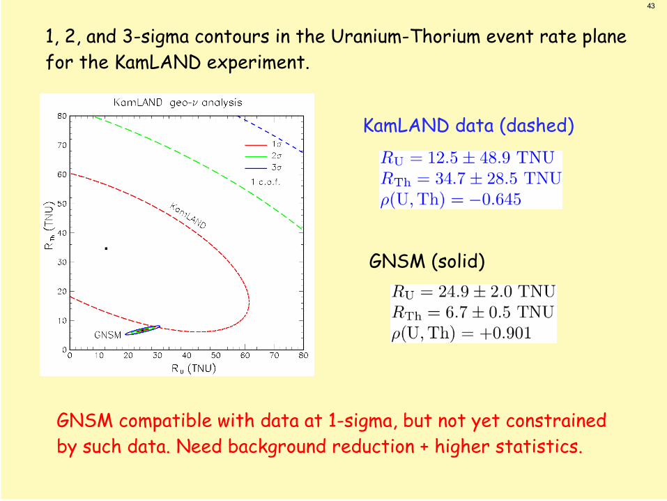
1, 2, and 3-sigma contours in the Uranium-Thorium event rate planefor the KamLAND experiment.

GNSM compatible with data at 1-sigma, but not yet constrainedby such data. Need background reduction + higher statistics.

KamLAND data (dashed)

GNSM (solid)

44

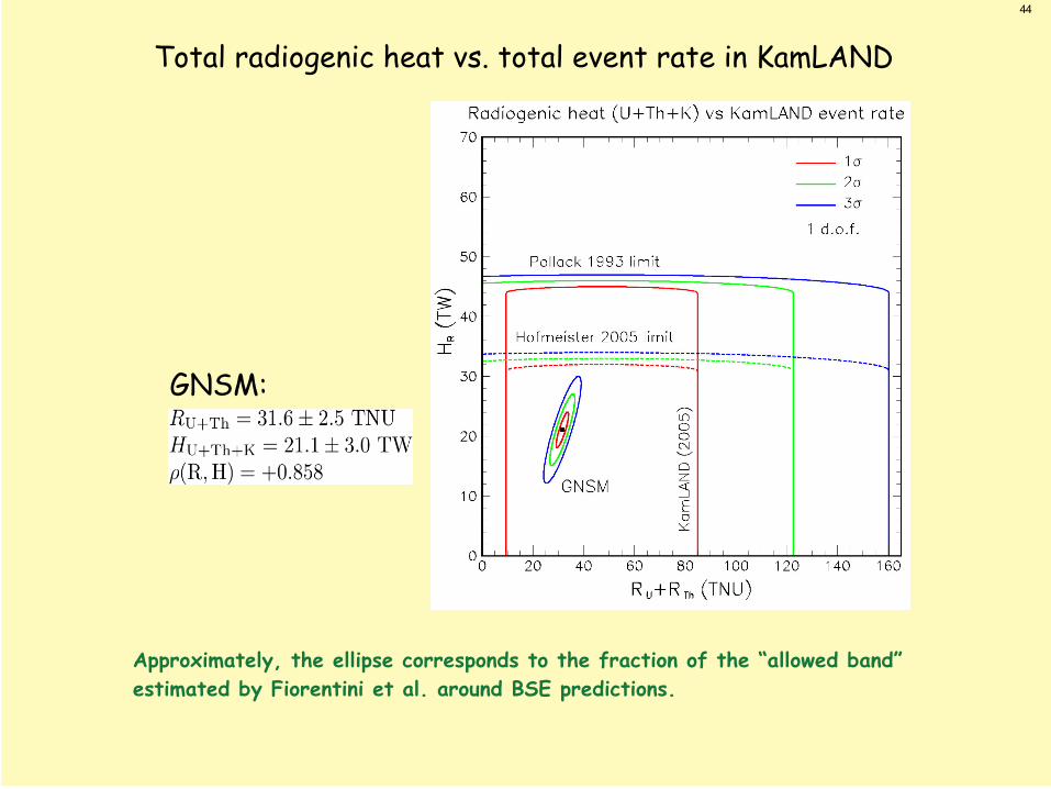
Total radiogenic heat vs. total event rate in KamLAND

Approximately, the ellipse corresponds to the fraction of the “allowed band”estimated by Fiorentini et al. around BSE predictions.

GNSM:

45

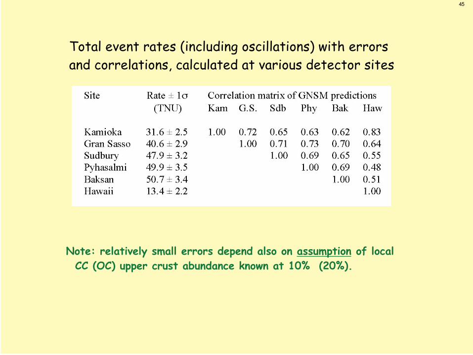
Total event rates (including oscillations) with errorsand correlations, calculated at various detector sites

Note: relatively small errors depend also on assumption of local CC (OC) upper crust abundance known at 10% (20%).

46

GNSM

Rate 1

Rate

2

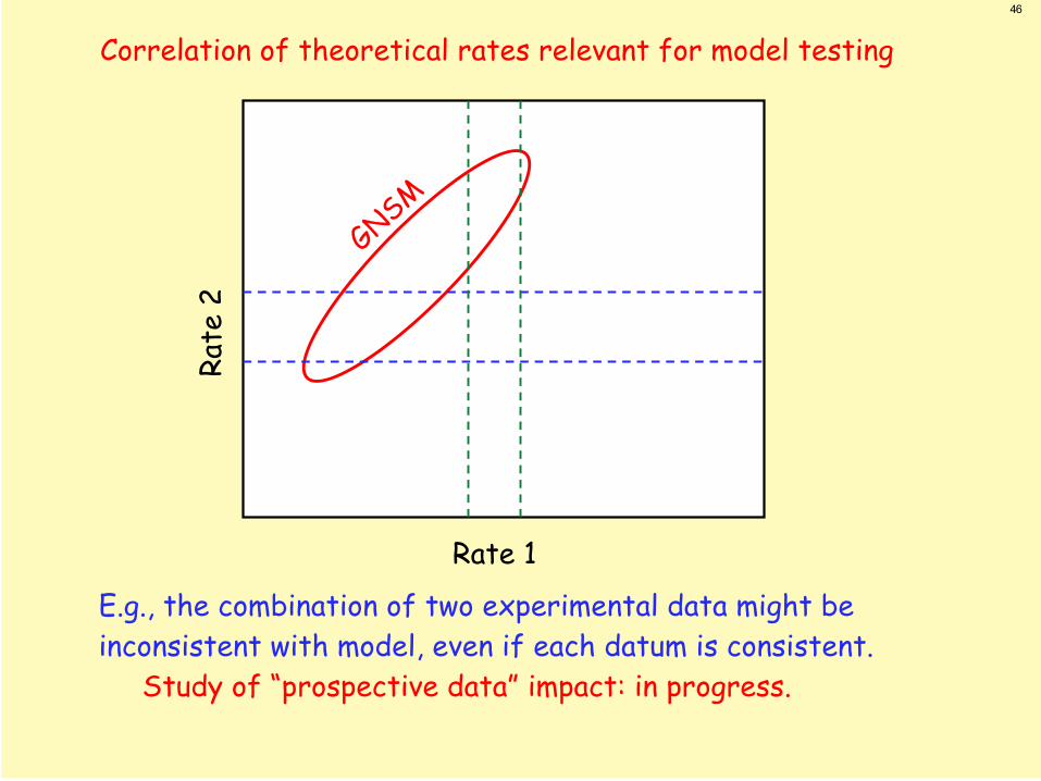
Correlation of theoretical rates relevant for model testing

E.g., the combination of two experimental data might beinconsistent with model, even if each datum is consistent. Study of “prospective data” impact: in progress.

47

ConclusionsCovariance analysis represents a useful “template” to embedcurrent and future information relevant to geoneutrino physics(it is already so in other neutrino research sub-fields)

We are still far from a satisfactory approach of this kind in(U,Th,K) geochemistry, due to intrinsic difficulties (large uncertainties, incomplete data, conflicting estimates, etc.) However, at least a tentative GNSM can be constructed

Improvements, especially for local contributions, crucial to assess quantitatively the impact of future expt’l data (and oftheir combination) on any GNSM (including non-orthodox ones)

Significant progress will benefit from joint, inter-disciplinary work by geophysicists, geochemists, and particle physicists