A Random Sampling Scheme

for Path Planning

J�erome Barraquand� Lydia Kavrakiy Jean-Claude Latombey Tsai-Yen Liz

Rajeev Motwaniy Prabhakar Raghavanx

June 24, 1996

Abstract

Several randomized path planners have been proposed during the last few years. Their at-tractiveness stems from their applicability to virtually any type of robots, and their empiricallyobserved success. In this paper we attempt to present a unifying view of these planners and totheoretically explain their success. First, we introduce a general planning scheme that consistsof randomly sampling the robot's con�guration space. We then describe two previously developedplanners as instances of planners based on this scheme, but applying very di�erent samplingstrategies. These planners are probabilistically complete: if a path exists, they will �nd one withhigh probability, if we let them run long enough. Next, for one of the planners, we analyze therelation between the probability of failure and the running time. Under assumptions character-izing the \goodness" of the robot's free space, we show that the running time only grows as theabsolute value of the logarithm of the probability of failure that we are willing to tolerate. Wealso show that it increases at a reasonable rate as the space goodness degrades. In the last sectionwe suggest directions for future research.

1 Introduction

Robot path planning has been proven a hard problem [40]. There is strong evidence that its solution

requires exponential time in the number of dimensions of the con�guration space, i.e., the number

of degrees of freedom (dofs) of the robot. This result is remarkably stable: it still holds for rather

speci�c robots, e.g., planar linkages consisting of links serially connected by revolute joints [17] and

sets of rectangles executing axis-parallel translations in a rectangular workspace [13, 14]. Though

general and complete algorithms have been proposed [6, 42], their high complexity precludes any

useful application. This negative result has led some researchers to seek heuristic algorithms.

�Salomon Brothers Int. Ltd., Victoria Plaza, 111 Buckingham Palace Road, London SW1W 0SB, UK. Email:

jerome.barraquand@sbil.co.uk.yDepartment of Computer Science, Stanford University, Stanford, CA 94305, USA. Email: fkavraki, latombe,

motwanig@cs.stanford.edu.zDepartment of Computer Science, National Chengchi University, Wenshan, Taipei, Taiwan. Email:

li@cs.nccu.edu.tw.xIBM Almaden Research Center, San Jose, CA 95120, USA. Email: pragh@almaden.ibm.com.

1

While several such planners solve di�cult problems, they also often fail or take prohibitive time on

seemingly simpler ones. The fact that their behavior is not well characterized is a major drawback:

they cannot be used as blackboxes in larger robot control systems.

The number of dofs beyond which existing complete algorithms become practically useless is low,

somewhere between 3 and 5. This means that they cannot be used to compute paths for rigid objects

translating and rotating in three dimensions, nor for six-dof manipulator arms, two important cases

in practice. On the other hand, robot applications tend to involve more degrees of freedom than

ever before. For example, an increasing number of manufacturing workcells use several cooperating

robots to augment throughput and exibility. Cells with more than twenty dofs are no longer

exceptions. As costs and time for designing and deploying them become more critical, path planners

integrated with CAD systems will be in higher demand to facilitate robot programming. Eventually,

planners will run online to allow for non-deterministic sequences of goals and events [31]. Robots

in domains other than manufacturing (e.g., medical surgery, space exploration) will also require

e�cient and reliable path planners. Some non-robotics domains raise a similar need as well. In

computer graphics, animation of synthetic actors to produce digital movies or video games requires

dealing with several dozen dofs. Here, motion planning may drastically reduce the work of human

animators who currently input large numbers of key frames. In molecular biology, motion planning

can help compute plausible docking motions of molecules modeled as spatial linkages with many

dofs.

Collision-free path planning, which assumes perfect knowledge of the world and stationary obstacles,

is only the most basic motion planning problem in robotics. Clearly, we would ultimately like

robot planners to also deal with issues such as uncertainties, moving obstacles, movable objects,

and dynamic constraints [29, 30]. But every extension of the basic problem adds in computational

complexity. For instance, allowing moving obstacles makes the problem exponential in the number

of moving obstacles [6, 41]; uncertainties in control and sensing make the problem exponential in

the complexity of the robot environment [6]. Before we can e�ectively investigate such extensions

in large con�guration spaces, it seems that we must better understand how to practically solve

basic path planning.

Path-planning applications are so diverse that it is infeasible to design a tailor-made algorithm

for every possible robot.1 Instead, we need general path planning algorithms not bound to the

speci�cs of any particular robot. We believe that between the two extreme types of planners

suggested above { complete and heuristic { there is place for practically e�cient general planners

achieving a weaker form of completeness. In other words, we may perhaps trade a limited amount of

completeness against a major gain in computing e�ciency. Full completeness requires the planner

to always answer a path-planning query correctly, in asymptotically bounded time. A weaker, but

still interesting form of completeness is the following: if a solution path exists, the planner will

�nd one in bounded time, with high probability. We call it probabilistic completeness. This weaker

completeness becomes particularly interesting if we can show that the planner's running time grows

slowly with the inverse of the failure probability that we are willing to tolerate.

With this philosophy in mind, we have designed new path planners and experimented with them

in large con�guration spaces. One of them, described in [3, 4, 29], is a potential-�eld-based planner

that escapes local minima by performing random walks; in the following, we will refer to it as the

1In any case, very few tailor-made planners have been successfully designed for speci�c robots with more than

four dofs.

2

potential-�eld planner. Another planner, presented in [18, 20, 21, 24], precomputes a \roadmap"

(network) of simple paths connecting randomly selected con�gurations and tries to construct a

path between any two input con�gurations by connecting them to this roadmap; we will refer

to this planner as the roadmap planner. Both these planners have been successfully applied to

complex problems. For example, in [26], the potential-�eld planner was used to automatically

synthesize a video clip with graphically simulated human and robot characters entailing a 78-

dimension con�guration space. Both the potential-�eld and the roadmap planners have been used

to check that parts can be removed from an aircraft engine for inspection and maintenance [8];

here, paths are generated in con�guration spaces having only six dimensions, but the parts have

particularly complex geometry.

These two planners achieve probabilistic completeness. For the potential-�eld planner, this property

remains qualitative: if there exists a path, the probability that the planner �nds one tends toward

one as the running time increases; but the convergence speed is unknown. But, for the roadmap

planner, we have proven stronger results that relate the probability that it �nds a path, when one

exists, to its running time [18, 19, 22, 23]. In turn, these theoretical results suggest improvements

of the planner.

Other work investigating similar or related randomized planning approaches include [1, 5, 15, 16,

35, 36]. Formal attempts to predict the behavior of speci�c random planners are proposed in very

few papers [9, 28].

This paper proposes a consistent framework to describe and study the randomized planners cited

above, with the goal to eventually build more powerful planners. In the planners cited above, the

robot's free space is not explicitly represented, but randomly sampled. We believe that this is

the central concept underlying their success. In Section 2 we capture this concept into a general

computational scheme for path planning in large con�guration spaces.2 In Section 3 we make our

discussion more precise by presenting our potential-�eld and roadmap planners as two instances of

planners using this scheme, but applying two di�erent sampling strategies. In Section 4 we give

two formal analyses of the probabilistic completeness of variants of the roadmap planner. These

analyses provide a theoretical explanation for the empirically observed success of the roadmap

planner. They are the crux of this paper. Indeed, as it has become relatively easy to design

new randomized path planners that outperform previous ones on some well-selected problems, it

is increasingly important to formally explain their strengths and weaknesses. This paper does

not present experimental results obtained with our planners. Many such results were previously

reported in [3, 8, 18, 20, 21, 24, 26, 27] and in papers by other authors [7, 11, 47]. The reader is

referred to [34] for a textbook on randomized algorithms and sampling techniques.

2 General Scheme

We consider the problem of planning collision-free paths for an arbitrary n-degree-of-freedom

holonomic3 robot A. We let C denote the con�guration space of A and Cfree stand for the open

subset of the collision-free con�gurations in C. We also refer to Cfree as the free space and to con�g-

2This scheme can also be applied to con�guration spaces having few dimensions; but it is less interesting in that

case, since complete algorithms are then available.3Our presentation can be extended to nonholonomic robots. See [36, 43, 44].

3

urations in Cfree as free con�gurations. A planning problem is speci�ed by two free con�gurations,

qinit and qgoal, called the initial and the goal con�gurations, respectively. Any path lying in Cfreethat joins these two con�gurations is a solution of this problem.

We assume for simpli�city that C is the cube [0; 1]n, so that each con�guration q is described by

an n-tuple (q1; : : : ; qn). However, it is straightforward to extend our presentation to cases where Cis multiply connected, i.e., one or more dimensions can \wrap around". The only requirement is

that C be measurable (in the Lebesgue sense), which is always achieved in practice.

Although there exist algorithms to construct an explicit representation of Cfree given the geometry

of A and the obstacles in semi-algebraic form, their time complexity makes them impractical for

any su�ciently large value of n. On the other hand, reasonably e�cient algorithms are available

to compute the Euclidean distance between two objects in three-dimensional space (e.g., [10, 32,

37, 39, 45]). This leads us to assume that Cfree is implicitly given by a function, clearance:

C ! R, that maps any con�guration q to the distance (in the workspace) between the robot placed

according to q and the obstacles, or between two bodies of the robot, whichever is smaller. In the

case where the robot collides with an obstacle or with itself, clearance(q) returns 0 or a negative

number. Thus, whenever clearance(q) is positive, q belongs to Cfree. We refer to clearance(q)

as the clearance of q.

For any bounded robot A, there exists a positive constant � such that when A moves along a

straight path in C between any two con�gurations q = (q1; : : : ; qn) and q0 = (q01; : : : ; q

0

n), no point

of A traces a curve segment longer than �maxi2[1;n] jqi�q0

ij. We assume here that � is given, though

for most usual robots its computation is straightforward and can be included in the planner. Rather

than using a single �, we may also partition C into several regions and have a distinct constant �ifor each region. If the �i's di�er by large amounts, this could substantially reduce the running time

of a planner based on the scheme presented below, but we will not go into such detail in this paper.

De�nition 1 Let q = (q1; : : : ; qn) and q0 = (q01; : : : ; q

0

n) be two free con�gurations whose respective

clearances are � and �0. They are said to be adjacent if �maxi2[1;n] jqi � q

0

ij < maxf�; �0g=2.

Clearly, if two con�gurations are adjacent the straight-line segment joining them lies entirely in

Cfree. In fact, the coe�cient 1=2 appearing on the right-hand side of the above inequality is

intended to make sure that the robot cannot collide with itself, since two bodies might then move

simultaneously toward each other. This coe�cient can be removed if self-collisions are known in

advance to be impossible. Note also that the map:

(q; q0) 2 C2 7! maxi2[1;n]

jqi � q0

ij 2 R+ [ f0g

is the L1 distance in C. We could choose other distances in C to de�ne adjacency. Of course, the

constant � depends on this choice.

Now we can state our general planning scheme as follows:

Pick con�gurations in C at random; retain those con�gurations which lie in Cfree (alongwith qinit and qgoal) as the nodes of a graph G; and connect adjacent con�gurations by

links of G.

Return yes if qinit and qgoal belong to the same connected component of G.

4

Return no if no path has been found after having generated c con�gurations, where c

is an input parameter.

The answer yes is always correct, that is, whenever the planner returns yes, there actually exists a

collision-free path connecting qinit to qgoal; moreover such a path can easily be extracted from the

graph G. But the answer no is not necessarily correct. Indeed, after a �nite amount of computation

(de�ned by the parameter c), the planner may still not have found a path between qinit and qgoal,

even if one exists.

The key component of this planning scheme is the sampling strategy applied to generate the nodes of

G. Di�erent strategies are possible. For example, if multiple planning queries are to be made with

the same robot and obstacles (multi-query case), then it may be suitable to invest preprocessing

time to construct a network of con�gurations (which we call a roadmap). Processing each query

then only requires connecting the input initial and goal con�gurations to the roadmap. If the

queries are not known in advance, it seems reasonable to construct the roadmap by choosing

con�gurations uniformly at random from [0; 1]n since the resulting free con�gurations are then

uniformly distributed over Cfree. However, we will see in Section 3.2 that, while the roadmap is

being generated, it is possible to derive heuristic information from it and bias the selection of the

new con�gurations.

Instead, if a single or very few queries are to be made with the same robot and obstacles (single-

query case), the planner may be more successful by using a sampling strategy that picks new

con�gurations, �rst in neighborhoods of the initial and goal con�gurations and then, iteratively, in

neighborhoods of the newly generated con�gurations, until the two \sampling waves" meet. A sim-

ilar strategy could also be used in the multi-query case to connect the initial and goal con�gurations

to the roadmap.

Although the e�ciency of any planner may be evaluated through experimentation, formal analysis

is desirable to compare planners and stress their strengths and weaknesses. Ideally a planner's

outcome should be yes with the highest probability whenever a free path exists and this outcome

should be generated in minimal time. Hence, the analysis should relate the probability that the

planner produces an incorrect answer to its running time. Given a small positive number � (the

acceptable probability that the planner's output is no while a free path exists), we would like to

bound the running time of the planner by a function of �. If this function grows slowly with 1=�,

then the planner is particularly interesting since we can get arbitrarily close to full completeness

at a reasonable cost.

Let us assume for simpli�city that clearance takes constant time to evaluate. Then the planner's

running time mainly depends on two numbers: the number of sample con�gurations and the number

of pairs of free con�gurations checked for adjacency. The number of sample con�gurations is at

most c. But only a fraction of them, f , are in Cfree, hence in the constructed graph G. In practice,

it is often the case that f � c. The planner should thus strive to get the greatest ratio f=c, but

the distribution of the generated free con�gurations is also crucial to eventually �nd a path. The

number of adjacency checks is at most proportional to f2; however, the planner may choose not to

test all pairs of free con�gurations for adjacency.4

4Checking the sample con�gurations for adjacency is an instance of the orthogonal range-searching problem [2, 38].

Using the range-tree technique, the pairs of adjacent con�gurations can be computed in O(f logn�1 f) time, or slightlyfaster. This is better than O(f2) when f is large enough.

5

It seems likely that no strong property can be proven for any given planner, if we do not make

some assumption about Cfree. Moreover, no single planner is likely to be the most e�cient for

all possible problems. This suggests that planners should be analyzed under some well-speci�ed

assumptions. In Section 4, we will study the work carried out by a two-phase planner under two

distinct assumptions. In one, the visibility volume assumption, Cfree is such that every free con�g-

uration \sees" a subset of Cfree whose volume is at least an � fraction of the total volume of Cfree(we then say that Cfree is �-good). In the second assumption, the path clearance assumption, there

exists a collision-free path between qinit and qgoal that has some given clearance �. Assumptions

must be carefully crafted. Indeed, if these are too speci�c or unrealistic, the analysis will not yield

useful results; on the other hand, if they are too general, the results will be too weak.

3 Speci�c Planners

We now present two planners that make use of the above scheme with di�erent sampling strategies.

3.1 Potential-Field Planner

This planner was originally described in [3, 4, 29], along with experimental results.5 Extensions

and additional experimental results were presented in [8, 11, 26, 27]. Here, we focus on its relation

to the general scheme presented above.

The planner is given a function U : Cfree ! R+ [ f0g, the potential �eld, with a single global

minimum (0) at the goal con�guration.6 It then attempts to connect qinit to qgoal by alternating

down motions and escape motions. Each down motion \descends" along U until it reaches a local

minimum, while escape motions attempt to ee from local minima.

The following algorithm, in which h is an input parameter, constructs a down motion starting at

con�guration qs:

Down-Motion(qs):

1. q qs.

2. While q is not labelled as a local minimum do:

(a) Pick at random up to h con�gurations adjacent to q, until one of them, q0, satis�es

U(q0) < U (q).

(b) If the previous step succeeded in generating q0, then reset q to q0; else label q as a local

minimum.

3. Return q.

At Step 2(a) let q = (q1; : : : ; qn) and � = clearance(q). Con�gurations are picked at random

from the volume de�ned by �i=1;:::;n[qi � �=�; qi + �=�] \ [0; 1]n. According to De�nition 1, all

con�gurations in this volume are adjacent to q. To guarantee that Step 2 does not loop for ever,

5The planner is available by anonymous ftp from flamingo.stanford.edu:/pub/li/rpp3d.tar.gz.6Techniques to automatically construct this function are proposed in [3, 29].

6

U must have no local minimum in the boundary of Cfree. This can easily be obtained by including

in the de�nition of U (q) a term proportional to 1/clearance(q).

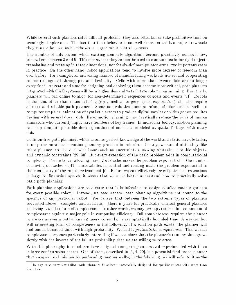
The following algorithm constructs an escape motion starting at a local minimum ql:

Escape-Motion(ql):

1. Pick at random the length, `, of the motion.7

2. q ql; l 0.

3. While l < ` do:

(a) Pick at random a free con�guration q0 adjacent to q.

(b) l l+ maxi jqi � q0

ij.

(c) q q0.

4. Return q.

The overall planning algorithm is the following:

Potential-Field-Planner(qinit; qgoal):

1. ql Down-Motion(qinit).

2. While ql 6= qgoal do:

(a) Do:

i. If the total number of con�gurations generated so far exceeds c then return no and

halt.

ii. qs Escape-Motion(ql);

iii. q0l Down-Motion(qs);

until U (q0l) < U(ql).

(b) ql q0

l.

3. Return yes.

The graph G constructed by the planner is a tree of paths rooted at qinit. Each con�guration

q0 entered as a node of G has been picked so that it is adjacent to a con�guration q already in

G (Steps 2(a) and 3(a) of Down-Motion and Escape-Motion, respectively). Moreover, q0 is only

linked to q in G. Hence, the planner does not test pairs of con�gurations for adjacency, avoiding

the cost of this test. During a down motion, the potential U introduces a bias in the choice

of the tree path that will be followed by the planner. Although the global geometry of Cfree is

unknown, U can be seen as a specialist that gives some heuristic indications about this geometry,

i.e.: which directions are promising and which aren't. The techniques in [3, 29] compute U by

7In [3], we note that, on the average, a random walk of length ` endsp` away from its starting point. This leads

us to suggest choosingp` according to a truncated Laplace distribution with mean value equal to the \radius" of

the con�guration space. Here, this radius is 1.

7

combining local-minima functions computed over the robot's workspace. Although the resulting U

often prevents the planner from getting trapped into big obstacle cavities, it still has local minima

and therefore is an imperfect characterization of the free space's geometry. On the other hand,

computing local-minima-free potentials in large dimensional spaces is a di�cult problem [25] that

is at least as hard as path planning itself.

Using well-known properties of random motions, the potential-�eld planner can be shown proba-

bilistically complete [3, 28]. Moreover, a calculation of the �nite expected number of invocations of

Escape-Motion is given in [28]. The idea underlying this calculation is the following. The basins

of attraction of the local minima of U which have non-zero measure (the goal basin is assumed to

be one of them) form a partition of the free space. For any two such basins Bi and Bj , one can

de�ne the �nite transition probability pij that a random walk generated by Escape-Motion from

the minimum in Bi terminates into Bj . The expected number of invocations of Escape-Motion

before entering the goal basin is then expressed as a function of the pij 's. In theory, this result

gives some indication of the expected complexity of the potential-�eld planner. But, in practice,

the pij 's are unknown. In fact, a key issue in analyzing a planner based on random sampling is to

translate some geometric property of the free space into probabilistic terms.

The potential-�eld planner has successfully solved many di�cult problems (e.g., see [3, 8, 11, 26]).

However, it is easy to create problems that it fails to solve in a reasonable amount of time, though

they admit rather obvious solutions. Not surprisingly, most failures are due to traps, which cause

some transition probabilities pij to be very small (in particular, the probabilities to enter the goal

basin from some other basins). A trap is a basin of attraction of a local minimum of U that is

almost completely surrounded by forbidden con�gurations (i.e., CnCfree). Hence, a trap admits

only narrow exits and the potential function inside the trap guides the robot away from these exits.

If the robot's path starts within a trap or is guided into one by U , each escape motion executed

then has a tiny probability of escaping the local minimum. One could imagine a variant of the

planner where the potential �eld is randomly guessed among a collection of several functions and

changed several times during planning, hoping that the various potentials would entail di�erent

traps. We did some experiments with this idea, but we only got limited results.

3.2 Roadmap Planner

The problems encountered with the potential-�eld planner led us to develop another planner, the

roadmap planner8 described in [18, 20, 21, 24]. Several variants of this planner have been im-

plemented; we present one below. Unlike the potential-�eld planner, this new planner uses no

problem-speci�c heuristics.

The roadmap planner operates in two phases, preprocessing and query processing: The preprocess-

ing phase consists of constructing a network R of con�gurations, the roadmap. The con�gurations

in R are called milestones. They only form a subset of all the sample con�gurations generated

by the planner; hence, the roadmap is not exactly the graph G mentioned in the general scheme.

Every query speci�es two con�gurations, qinit and qgoal, in Cfree. Processing the query consists

of connecting these con�gurations to two milestones and checking that these two milestones are in

the same connected component of R.

8The planner is available by anonymous ftp from flamingo.stanford.edu:/pub/kavraki/prm.tar.gz.

8

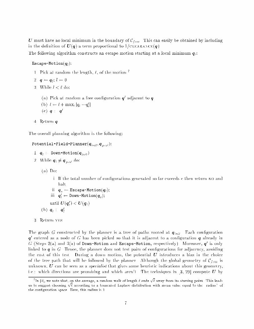
The planner uses a simple algorithm, Connect (also called the connector), to construct the links ofR.

Given any two milestones,m1 andm2, the connector checks if the straight-line segment connecting

them lies in Cfree. It does so by dichotomically breaking the segment into shorter segments and

checking the endpoints of each segment for adjacency. It stops breaking a segment whenever its

two endpoints are adjacent or one of them is not in free space. In the second case, Connect

halts, without generating a link between m1 and m2 in the roadmap. Instead, if the connector

eventually succeeds in partitioning the segmentm1m2 into segments (possibly, of unequal lengths)

such that the endpoints of each segment are adjacent, it establishes a link between m1 and m2 in

the roadmap. The work done by the connector is part of the sampling work done by the roadmap

planner, but the sample con�gurations it generates are not permanently stored; they are not part

of the roadmap R. In other words, the planner does not attempt to �nd additional connections

among sample con�gurations generated between milestones. To keep our presentation simple, we

assume that Connect only tries straight paths, but it could try other canonical paths as well. We

say that a con�guration sees another con�guration if the straight-line segment joining them lies

entirely in Cfree.

In the following algorithm we could limit the total number of sample con�gurations to c, as in the

general scheme of Section 2. However, putting the limit on the number of generated milestones

instead is more convenient; it will also facilitate the analyses of Section 4. The preprocessing phase

constructs an initial roadmap containing r milestones (Steps 2 and 3 in the algorithm shown below).

Then it expands this initial roadmap into a �nal one containing s > r milestones. Both r and s

are input parameters. The �rst r milestones are chosen uniformly over Cfree. The remaining s� r

milestones are selected in small regions considered as \di�cult" parts of Cfree. The preprocessingalgorithm is the following:

Preprocessing:

1. i 0.

2. While i < r do:

(a) Pick a con�guration q in C at random.

(b) If clearance(q) > 0 then

i. Store q as a milestone of the roadmap.

ii. i i+ 1.

3. For every pair of milestonesm1 andm2 whose distance is less than d, do: Connect(m1;m2).

4. Invoke Resample to expand the roadmap by s� r milestones (see below).

The threshold d at Step 3 is an input parameter. It is used to limit the number of pairs of milestones

that are tested by Connect, since in most spaces two milestones that are far apart are unlikely to

see each other. Step 3 takes time at most quadratic in r, which is usually much smaller than the

total number of sample con�gurations generated by the roadmap planner.9

Resample selects milestones with probability inversely proportional to their degrees in the roadmap

(i.e., their number of connections to other milestones). Intuitively, a milestone with few or no

9Footnote 4 applies here too.

9

connections lies in a di�cult region of the free space. For each milestonem that it selects, Resample

picks a number of new milestones at random in a neigborhood ofm and invokes Connect to try to

link each of these new milestones to other milestones. This expansion of the roadmap terminates

when the total number of milestones is s. Experiments have been done with and without the

roadmap expansion step (Step 4). Roadmaps containing the same total number of milestones

have been constructed both ways. The roadmaps generated using the expansion step have been

consistently better, i.e., subsequent queries were processed more quickly with less incorrect no

answers. Over a large range of problems, generating 2/3 of the milestones at Step 2 and 1/3 at

Step 4 gave good results.

After preprocessing, each query is handled as follows (g is an input parameter):

Query-Processing(qinit; qgoal):

1. For i = finit; goalg do:

(a) If there exists a milestone m that sees qi then mi m.

(b) Else

i. Repeat g times:

Pick a con�guration q at random in the neighborhood of qi

until q sees both qi and a milestone m.

ii. If all g trials failed then return no and halt, else mi m.

2. If minit and mgoal are in the same component of the roadmap then return yes; else return

no.

4 Analysis

We now give formal analyses of two variants of the roadmap planner. We characterize the amount

of computation that the planner must do in order to give correct answers with high probability.

The intuitive reason for the experimental success of the above planners is that there usually exist

many collision-free paths joining two con�gurations. Hence, to bound the running time of the

roadmap planner, we assume that Cfree satis�es some geometric property capturing the above

intuition. We propose two such properties. Our thesis is that the success of any sampling strategy

will stem from a similar property.

In both analyses, we consider that the key number a�ecting the planner's running time is the

number of milestones in the constructed roadmap. Since to generate a single milestone it might be

necessary to randomly pick several (possibly, many) con�gurations in C, we implicitly assume that

the volume of Cfree relative to the volume of C is not too small. If this assumption is not satis�ed,

any variant of the roadmap algorithm presented in Section 3.2 will behave poorly. In this case, we

should probably make the additional assumption that a few free con�gurations are given (after all,

every query will give two such con�gurations); then, a possible sampling strategy could be to build

a roadmap by generating milestones in small regions centered at the given con�gurations, �rst, and

at the newly generated milestones, next.

10

Note that bounding the number of milestones is not su�cient to bound the running time of the

planner, because it does not account for the running time of Connect. If two milestones passed

to Connect see each other, but the line segment connecting them is arbitrarily close to the free

space boundary, then the connector will have to break it into arbitrarily many small segments.

This problem could be eliminated by extending the general scheme of Section 2 with a primitive

computing the volume swept out by the robot when it moves between two con�gurations along a

straight path in con�guration space.

Here, we only state the main results of our analyses. We give formal proofs of the three main

theorems (Theorems 1, 2, and 7) in the appendix. The proofs of two other theorems (Theorems 3

and 4) are straighforward and short; they appear in the text below. For the proofs of Theorems 5

and 6, we refer the reader to [22, 23]. Indeed, these proofs are longer and more technical, while the

theorems themselves are less important to a robotics audience. Finally, Theorem 8 is essentially a

re�nement of Theorem 7. Its proof can be found in [18, 19].

In the rest of this section we denote the volume of a subset X of C by �(X ).

4.1 Visibility Volume Assumption

4.1.1 De�nition and algorithms

For any con�guration q 2 Cfree, let S(q) consist of all those con�gurations q0 2 Cfree that q sees.

De�nition 2 Let � be a positive real. A con�guration q 2 Cfree is �-good if �(S(q)) � ��(Cfree).Furthermore, Cfree is �-good if all the con�gurations it contains are �-good.

The visibility volume assumption made here is that Cfree is �-good, that is, each con�guration in it

sees a signi�cant portion of Cfree. The underlying intuition is that it is then relatively easy to pick

a set of milestones that, collectively, can see most of Cfree. But the assumption fails to prevent

Cfree from containing narrow passages through which it might be di�cult to connect milestones.

For example, consider the case where C is two-dimensional and Cfree consists of two disks of equalsize that overlap by a very small amount. Then Cfree is �-good for � � 0:5. But the probability

that any milestone in one disk sees a milestone in the other disk is very small. For this reason, we

use a variant of the roadmap algorithm that embeds a \complex planner". We assume that this

complex planner is error-free in that it discovers a path between two given con�gurations whenever

one exists, and reports failure when there is none. But of necessity such a complete planner must

be expensive to run, and so we seek to use it sparingly. In particular, to keep query processing fast,

we restrict the use of the complex planner to the preprocessing stage.

The preprocessing algorithm is similar to the one given in Section 3.2. The main di�erence is that

Step 4 invokes Permeation, instead of Resample. Permeation uses the complex planner to improve

the roadmap connectivity; unlike Resample, it does not add new milestones to the roadmap. The

constructed roadmap contains s milestones; these are all generated at Step 2.

Preprocessing:

1. i 0.

2. While i < s do:

11

(a) Pick a con�guration q in C at random.

(b) If clearance(q) > 0 then

i. Store q as a milestone of the roadmap.

ii. i i+ 1.

3. For every pair of milestones m1 and m2, do: Connect(m1;m2).

4. Pick one representative milestone from each component of the current roadmap. Let V be

the set of these representative milestones. Invoke Permeation(V ) to improve the connectivity

of the milestones (see below).

The result of this preprocessing is a roadmap such that any two nodes are in the same component

if and only if the corresponding milestones are in the same component of Cfree. Step 3 may

fail to �nd all possible links between the milestones due to the incompleteness of the connector.

Permeation invoked in Step 4 �xes this problem by using the complex planner to discover additional

connections between milestones. Note that Permeation is a last resort; hopefully, much if not all

of the connectivity information should have been discovered before this step.

It is worth noticing that the algorithms of the implemented planner presented in [18, 20, 21]

are similar to those described here, except that it uses the potential-�eld planner of Section 3.1

instead of the complex planner. The potential-�eld planner is not complete, but it is quite rare in

practice that two milestones in the same component of the free space can be connected neither by

invoking Connect at Step 3 of the proprocessing, nor by the potential-�eld planner. The planner

of [18, 20, 21] seems a good approximation of the algorithms given here, and the analysis proposed

below is relevant to this planner.

The query processing is handled by the following algorithm, which is similar to the query-processing

algorithm of Section 3.2:

Query-Processing(qinit; qgoal):

1. For i = finit; goalg do:

(a) If there exists a milestone m that sees qi then mi m.

(b) Else

i. Repeat g times:

Pick a con�guration q at random in S(qi)

until q sees both qi and a milestone m.

ii. If all g trials failed then return failure and halt, else mi m.

2. If minit and mgoal are in the same component of the roadmap then return yes; else return

no.

Step 1(b)i di�ers slightly from the corresponding step in the query-processing algorithm of Sec-

tion 3.2. Since in general we do not know how to compute S(qi), picking con�gurations in this set

requires guessing con�gurations in con�guration space and retaining only those that are seen by

qi. This means that each of the g iterations performed at Step 1(b)i may require several trials to

12

obtain a con�guration visible from qi. The analysis proposed below ignores these trials and focuses

only on the number g.

Another di�erence between the above algorithm and the one of Section 3.2 is that it returns failure

(instead of no) at Step 1(b)ii. Due to the use of the Permeation in the preprocessing, both the

answers yes and no are now always correct. With some probability though, the query-processing

algorithm may fail to give an answer.

4.1.2 Performance guarantees

Let us �rst present some performance guarantee for the preprocessing phase. Call a set of milestones

adequate if the volume of the subset of Cfree not visible from any of these milestones is at most

(�=2)�(Cfree). Intuitively, if we were to place a point source of light at each milestone, we would

like a fraction at least 1� �=2 of Cfree to be illuminated.

Let C be a positive constant large enough that for any x 2 (0; 1], (1�x)(C=x)(log1=x+log2=�) � x�=2.

Clearly, there exists such a constant.

Theorem 1 Let � 2 (0; 1] be a positive real constant. If s � (C=�)(log 1=�+ log 2=�), then prepro-

cessing generates an adequate set of milestones with probability at least 1� �.

Note that as � increases, the requirement for adequacy grows weaker, i.e., the portion of the free

space that has to be visible by at least one milestone gets smaller. Intuitively, this comes from the

fact that a greater � will make it easier to connect query con�gurations to the roadmap. Naturally,

the number of milestones needed becomes smaller.

Theorem 1 only says that most of Cfree is likely to be visible from some milestone in the roadmap;

using this property alone, we can show that queries can be answered quickly. But the adequacy of

the milestones is not su�cient to imply that the roadmap is a good representation of the connectivity

of Cfree. The use of the complex planner in the permeation algorithm is inevitable to ensure a good

probability that the query processing outcomes yes or no.

Let us choose g = log(2= ) at Step 2 of Query-Processing, where 2 (0; 1] is the failure probability

we are willing to tolerate during a query. We can show the following performance guarantee for

the query processing phase:

Theorem 2 If the set of milestones chosen during preprocessing is adequate, then the probability

that the query-processing algorithm outputs failure is at most .

In fact, our analysis (in the Appendix, Section B) implies that the expected number of executions

of Step 1(b)i in the query-processing algorithm is at most 2.

Theorems 1 and 2 give performance guarantees for the preprocessing phase and the query-processing

phase, respectively. This is appropriate, since many queries will be made using the same roadmap.

However, we can easily blend the two theorems to bound the probability that the planner returns

failure for a single query by (1 � �) + � (this is obtained by bounding by one the probability

that the planner returns failure when the set of milestones is not adequate). Then, let � 2 (0; 1]

be the probability of a failure outcome which we are willing to tolerate. Neither the number s of

milestones, nor the number g of trials at Step 2 of Query-Processing grow faster than log(1=�),

when �! 0.

13

4.1.3 Number of calls to complex planner

We now turn to the description of Permeation and its analysis. Our goal is to evaluate how many

times the complex planner must be invoked at Step 4 for the preprocessing algorithm.

Permeation must determine which milestones in V are reachable from each other, i.e., it must

partition V into subsets such that all milestones in the same subset belong to the same component

of Cfree and no two milestones in two di�erent subsets are in the same component of Cfree. If p is

the size of V , it can do so with O(p2) invocations of the complex planner by trying it on every pair

of milestones in V , but we show below that far fewer invocations may su�ce.

We work with the following abstract version of the permeation problem. The input is a graph N

with p vertices, consisting of k disjoint cliques. The goal is to determine this clique partition of N .

The graph is presented as an adjacency matrix and the cost of an algorithm is measured by the

number of entries it examines in the adjacency matrix of N . This is the edge probe model used in

the study of evasive graph properties [33]. The vertices of N correspond to the milestones in V , and

an edge is present between two vertices if the corresponding milestones lie in the same component

of Cfree. The milestones from any particular component of Cfree will form a clique in N , and there

are no edges between two distinct cliques. A probe into the adjacency matrix corresponds to an

invocation of the complex planner.

Let NC(p; k) denote the non-deterministic complexity of this problem. A non-deterministic algo-

rithm is only required to verify that some partition into k cliques is the right partition. It must

make at least one probe on each of the p vertices. It must also have veri�ed that each of the

k

2

!

pairs of cliques is in fact disconnected. Hence:

Theorem 3 For 1 � k � p, NC(p; k) = �(p+ k2).

The non-deterministic complexity of the problem is clearly a lower bound on its deterministic and

even randomized complexity.

We now characterize the worst-case deterministic complexity of this problem, denoted T (p; k).

Consider the following deterministic algorithm: by probing all edge slots incident on an arbitrary

vertex x, determine the neighborhood of x, say �(x); let Cx = fxg [ �(x), and output Cx; then,

recur on the vertex-induced subgraph N [V n Cx]. The number of levels in the recursion is k, since

one of the k cliques is removed from N prior to each recursive call. The number of probes made

in the process of determining each such clique is at most p. The total number of probes is O(pk).

The following permeation algorithm is an iterative version of the recursive algorithm (the nodes of

N are named 1; 2; : : : ; p):

Deterministic-Permeation(V ):

1. Mark all vertices of N as being live.

2. Initialize x 1.

3. While x � p do:

(a) �(x) ;.

14

(b) For y = x+ 1 to p do:

i. If vertex y is marked live then probe the edge (x; y) in N .

ii. If edge (x; y) is probed and found present then mark y as dead and add y to �(x).

(c) Output fxg [ �(x) as being a clique.

(d) Mark x as being dead.

(e) Set x to the smallest numbered live vertex, or p+ 1 if there are no live vertices left.

By the preceding discussion, we have:

Theorem 4 Deterministic-Permeation correctly solves the permeation problem using O(pk)

probes.

The following lower bound establishes that Deterministic-Permeation is optimal. The proof uses

a non-trivial adversary argument [23].

Theorem 5 For 1 � k � p, T (p; k) = (pk).

We now give a randomized algorithm that beats the lower bound of Theorem 5 when

the sizes of the k cliques di�er signi�cantly, which is often the case in practice (when

k > 1). Randomized-Permeation labels the vertices in a random order and then invokes

Deterministic-Permeation.

Randomized-Permeation(V ):

1. Permute the vertices randomly. Rename the nodes by 1; : : : ; n, in the order of the generated

list.

2. Invoke Deterministic-Permeation(V ).

Let w1 � w2 � � � � � wk be the sizes of the cliques in an instance N arranged in a non-increasing

order, where p =Pk

i=1wi. Denote by Ci the ith largest clique in N . De�ne a function u() on an

ordered k-tuple of positive integers n1; n2; : : : ; nk by u(n1; n2; : : : ; nk) =Pk

i=1 ini.

Theorem 6 Randomized-Permeation correctly determines the clique structure and incurs an ex-

pected cost that is at most

2u(w1; w2; : : : ; wk)� p� k:

Furthermore, with high probability, the cost is at most

O(u(w1; w2; : : : ; wk) log p):

Observe that the worst case is when all wi are equal to p=k, in which case the expected cost is

O(pk). On the other hand when there is one giant clique and k�1 cliques of size O(1) the expectedcost is �(p+ k

2), which is essentially the non-deterministic lower bound.

15

4.2 Path Clearance Assumption

The visibility volume assumption does not prevent the existence of narrow passages in Cfree. To

remove the need for the \complex planner" and get closer to the roadmap planner of Section 3.2,

we now consider a seemingly stronger assumption: between the two con�gurations given by a

query, there exists a collision-free path � that achieves some clearance � between the robot and the

obstacles. More formally, let us parametrize � by the arc length ` from the initial con�guration

and let L designate the path's total length, i.e., � : ` 2 [0; L]! �(`) 2 Cfree. We de�ne �(`) to be

the Euclidean distance between �(`) and the free space boundary, and �inf to be inf `2[0;L] �(`).

We consider a variant of the roadmap planner in which the preprocessing algorithm consists of the

�rst three steps of the algorithm given in Section 4.1. Unlike the planner of Section 3.2, it does not

include the resampling step. The query-processing algorithm is also simpler than in Section 3.2, in

that it only checks that the initial and goal con�gurations see milestones in the roadmap. If any one

of these connections fails, the query-processing algorithm returns no. Hence, this query-processing

algorithm is deterministic.

Under the path clearance assumption, any no outcome is incorrect. Let � be the probability that

we are willing to tolerate for this event. The following two theorems relate the size of the roadmap

to this probability, as well as to the two parameters of the assumption, that is, the length L of the

hypothesized path and its clearance. They give a performance guarantee for the whole planner.

Theorem 7 Let � 2 (0; 1] be a positive real constant. Let a be the constant 2�n�(B1)=�(Cfree)

where B1 denotes the unit ball in Rn. If s is chosen such that:

2L

�inf(1� a�

ninf )

s � �; (1)

then the planner outputs yes with probability at least 1� �.

Note that, for any given L and �inf , the quantity on the left side of the above inequality tends

toward zero when s ! 1. It is even more important to remark that it depends exponentially on

s, so that the number of milestones s needed grows no faster than the logarithm of 1=�.

The following theorem is similar to the previous one, but makes use of the clearance distribution

�(`) rather than just its in�mum:

Theorem 8 Let � 2 (0; 1] be a positive real constant. Let a be the same constant as in Theorem 7.

If s is chosen such that:

6

Z L

0

(1� (a=2n)�n(`))s

�(`)d` � �; (2)

then the planner outputs yes with probability at least 1� �.

Using the inequality 1� x � e�x, for x � 0, we get the following easier-to-use relations:

� The bound of Theorem 7 becomes:

2L

�infexp(�a�ninfs) � �: (3)

16

0 10

1

2ω

ω

ωq

q

init

goal

τ

Figure 1: Illustrative example

� The bound of Theorem 8 becomes:

6

Z L

0

exp(�a2�n�n(`)s)

�(`)d` � �: (4)

Relation 3 implies that the number of milestones that the planner must generate to output yes

with probability at least 1� � is polynomial in 1=�inf and logarithmic in L.

Remark that �(`) � (1=2�) clearance(�(`)), where � is the constant introduced in Section 2.

Indeed, for any q 2 Cfree, let qc be the con�guration in the free space boundary that achieves

minimum distance with q and let �(q) be this distance. We have: �(q) � maxi jqi � qci j. By the

de�nition of �, all con�gurations q0 such that maxi jqi � q0

ij � clearance(q)=2� are in the free

space. Hence, clearance(q)=2� < maxi jqi � qci j � �(q). Therefore, the bounds given above

remain valid if we choose to de�ne �(`) as (1=2�) clearance(�(`)), rather than as the distance

between �(`) and the free space boundary.

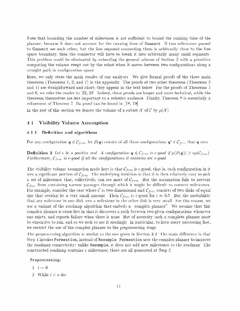
4.3 Example

Consider the two-dimensional problem (n = 2) shown in Figure 1. This problem is parametrized

by !. The walls are obstacles, but have zero thickness; hence, �(Cfree) = 1. We are interested in

the order of magnitude of s when ! is small. Let x � y mean that (1=C)x � y � Cx for some

constant C > 0. In particular, we have L � 1 and �inf � !.

Estimate of s using Theorem 1: The space in Figure 1 is �-good for � = 2!2 (clearly, because

of the \box" on the left). In order to bound the probability that the query-processing algorithm of

section 4.1 outputs failure, while a collision-free path exists (Theorem 2), the roadmap must be

adequate. According to Theorem 1, this is achieved with high probability if:

s �1

!2log

1

!: (5)

17

Estimate of s using Theorem 7: Using (3) we can derive the following order of magnitude for

s that will make the planning algorithm of Section 4.2 to return yes with high probability [19]:

s �1

!2log

1

!: (6)

Estimate of s using Theorem 8: The bound given by (4) leads to choosing (see [19]):

s �1

!2log log

1

!: (7)

Comparison: Note that to answer queries with high probability it is necessary and su�cient in

this example to pick a bounded number of milestones in the box, which happens with probability

� !2. Hence, a tight estimate of s is

s �1

!2:

The estimates (5), (6), and (7) can be seen as the unavoidable quantity 1=!2 times some factor.

By exploiting the fact that �(`) is small only brie y, we get a smaller factor in (7) than in (6).

5 Discussion

Between complete planners, which take prohibitive time to run in large dimensional con�guration

spaces, and ad hoc planners, which are too unreliable, there exist planners that are reasonably

e�cient while achieving some form of completeness. In this paper we have discussed a class of such

planners. These are based on a general computational scheme presented in Section 2, which consists

of randomly sampling the free space and checking pairs of sample con�gurations for adjacency. By

choosing an appropriate sampling strategy, this scheme can be turned into a concrete planner that

achieves probabilistic completeness. In Section 3 we have presented two examples of probabilistically

complete planners: the potential-�eld and the roadmap planners. In Section 4 we have analyzed in

more detail the probabilistic completeness of variants of the roadmap planner, under two di�erent

assumptions: the visibility volume assumption and the path clearance assumption. In each case,

we have established a relation between the probability that the planner �nds a path, when one

exists, and its running time (measured in that case by the number of milestones in the roadmap).

Both analyses show that the number of milestones needed grows only as the absolute value of the

logarithm of the probability of an incorrect answer that we are willing tolerate. Moreover, this

number is polynomial in the inverse of the parameter used to measure the goodness of free space

(� in the �rst analysis, �inf in the second).

How realistic and useful are our assumptions? Clearly, in most cases, there is no pratical way to

verify that they are satis�ed. Furthermore, it is easy to create spaces that are �-good for very small

values of �, as well as spaces that are not �-good for any positive value of �. For instance, this is

the case of the space comprised between two circles C1 and C2 tangent at some point P , with C2

contained in C1. On the other hand, in many applications, we are willing to discard collision-free

paths if their clearance is too small, due to uncertainties in robot control and sensing. In those

cases, a planner that would return a path with high probability, whenever there exists one that has

18

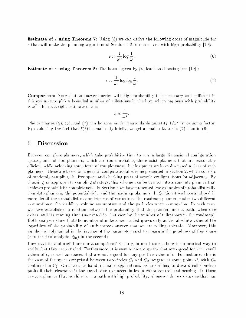
Figure 2: Robot arm example

enough clearance, would be quite satisfactory.10 Remark also that, if there exists a collision-free

path with a clearance greater than some given �inf , this path must lie in a subset of Cfree that isat least �-good for an � that can be derived11 from �inf . Hence, the assumption of �-goodness is

realistic as well: for any given value of �, our analysis characterizes the probability that the planner

�nds a path in the subset of Cfree that is �-good.

But we think that much more could be done. In particular, neither of the two analyses we have

given considers the resampling step (Step 4) in the preprocessing algorithm of Section 3.2. On

the other hand, our experiments have shown that adding this step yields a much better roadmap

planner. In relation to this observation, we have empirically tested the free space corresponding to

the setting of Figure 2 (a seven-revolute-dof planar arm among several barriers forming multiple

gates) for �-goodness. To do so we have picked 9,000 milestones at random and we have computed

how many other milestones each milestone can see. The milestones with the \most" visibility could

only see about 0:06 (i.e., 6%) of the remaining milestones, suggesting that they are 0:06-good. As

many as 3:3% of the milestones could see no other milestones, and fully 22% could see 0:001 (i.e.,

0:1%) or less; in other words, only about 78% of the con�guration space is 0:001-good or better.

On the other hand, the implemented planner, which includes the resampling step, handles queries

in this setting with quasi-perfect reliability, after having constructed a roadmap containing 5,000 to

10,000 milestones. Other experiments con�rm that the use of Resampling improves the coverage

of the free space by the milestones.

To explain the role of Resampling we introduce a generalization of the notion of �-goodness. We

say that a free con�guration q is (�; 1)-good if �(S(q)) � ��(Cfree), corresponding to our original

de�nition of �-goodness for a con�guration. Next, we say a free con�guration q is (�; t)-good if

�(fq0 2 S(q) j q0 is (�; t� 1)-goodg) � �(S(q))=2. For t > 1, we say that Cfree is (�; t)-good if

�(fq 2 Cfreejq is (�; 1)-goodg) � �(Cfree)=2 and every free con�guration is (�; i)-good for i � t.

If Cfree is (�; t)-good for a small value of t, we can give a theoretical basis for the resampling

strategy. The main idea is that single links discovered by the connector in the algorithms are now

simulated using t-link paths found by resampling and connecting using the connector. This leads to

a generalized de�nition of an adequate set of milestones, and eventually to a version of Theorem 2

10Note that the roadmap planner may nevertheless return a path with a smaller clearance.11However, the bound derived from �inf may be much smaller than the actual �. E.g., if the free space is a rectangle

having very small width �, then �inf � �, but � = 1.

19

in which the number of invocations of the connector is larger by a factor of 2t. See [23] for more

detail.

We believe that future research should develop and analyze new sampling strategies, as well as

combinations of strategies, under various assumptions. In particular, it would be of particular

interest to investigate strategies suitable for single-query planning problems. In this case, instead

of spreading milestones all over the free space, one could expand a \cloud" of sample con�gurations

from the initial con�guration toward the goal, or in both directions concurrently. This could be

achieved by iteratively generating con�gurations in small neighborhoods of previously generated

con�gurations, while keeping only those con�gurations which are in the same free space component

as the initial con�guration. This strategy could use a function similar to a potential �eld as a

probability distribution to randomly choose which con�gurations to expand from at every iteration.

In the multi-query case, it would also be useful to consider the case where all queries are made in

the same component of Cfree and the preprocessing is given one con�guration in that component.

The case where the volume of the free space is very small relative to the total volume of the

con�guration space should also be investigated. We envision that ultimately randomized planners

will automatically select and combine sampling strategies from a library of basic strategies to closely

match the characteristics of the input problems. This sort of combination has already given good

results in another area, graphic rendering [46].

We did not discuss distance calculation in this paper, but it is a key computation in the context of

our sampling scheme. Indeed, our planners spend most of their time evaluating clearance. So,

any improvement of the time e�ciency of the algorithm implementing clearance would translate

into a planning improvement of the same order of magnitude. One could also try to match the

distance calculation algorithm and the sampling strategy, to get the best global result. For exam-

ple, a sampling strategy generating con�gurations in small neighborhoods of previously generated

con�gurations could be combined with an incremental distance calculation algorithm such as the

one proposed in [32]. Such an algorithm uses the nearest points computed at the previous con�gu-

ration to quickly �nd the nearest points at the new con�guration. As another example, the distance

calculation algorithm proposed in [39] (and used in our planners) precomputes data structures to

later accelerate the processing of distance calculation queries. Each such data structure is a binary

tree of spheres approximating a single rigid body. Given two bodies, a simple traversal of their

respective trees allows us to quickly detect collision or identify the nearest points between the two

bodies. A perhaps more e�cient solution would be to create a single data structure for all the rigid

bodies forming the robot and to e�ciently update this data structure when con�guration parame-

ters vary (as proposed in [12]). Then the sampling strategy should try to generate con�gurations

in a sequence that minimizes update costs.

The random sampling scheme for path planning proposed in this paper o�ers many opportunities

for further research. We are con�dent that it can ultimately produce very fast planners able to

correctly handle a wide range of problems with high probability.

Acknowledgments: The development of the potential-�eld and roadmap planners has been supported by

ARPA contracts DAAA21-89-C0002, N00014-92-J-1809, and N00014-94-1-0721. The formal analysis of these

planners and the design of the general random sampling scheme was supported by MURI grant DAAH04-

96-1-0007 (Army). The experimental part of this research has also bene�ted from gifts by General Electric,

General Motors, Renault, and Rockwell. Lydia Kavraki and Jean-Claude Latombe are partially supported

20

by ARPA contract N00014-94-1-0721 and a MURI grant of the Army. Rajeev Motwani is supported by

an Alfred P. Sloan Research Fellowship, an IBM Faculty Partnership Award, and NSF Young Investigator

Award CCR-9357849, with matching funds from IBM, Schlumberger Foundation, Shell Foundation, and

Xerox Corporation. This paper has bene�ted from useful comments by Leo Guibas, Dan Halperin, and

Jean-Paul Laumond.

References

[1] J.M. Ahuactzin Larios, Le Fil d'Ariane: Une M�ethode de Plani�cation G�en�erale. Application �a laPlani�cation Automatique de Trajectoires, Th�ese de l'Institut National Polytechnique de Grenoble,

Septembre 1994.

[2] S. Arya and D.M. Mount, Approximate Range Searching, Proc. of ACM Symp. on ComputationalGeometry, 172-181, 1995.

[3] J. Barraquand and J.C. Latombe, Robot Motion Planning: A Distributed Representation Approach,

The Int. J. of Robotics Research, 10(6):628-649, 1991.

[4] J. Barraquand, B. Langlois, and J.C. Latombe, Numerical potential Field Techniques for Robot Path

Planning, IEEE Tr. on Syst., Man, and Cyb., 22(2):224-241, 1992.

[5] P. Bessi�ere, E. Mazer, J.M. Ahuactzin, Planning in a Continuous Space with Forbidden Regions: The

Ariadne's Clew Algorithm, Algorithmic Foundations of Robotics, K. Goldberg et al. (eds.), AKPeters,

Wellesley, MA, 39-47, 1995.

[6] J.F. Canny, The Complexity of Robot Motion Planning, MIT Press, Cambridge, MA, 1988.

[7] D. Challou and M. Gini, Parallel Formulation of Informed Randomized Search for Robot Motion Plan-

ning Problems, Proc. of IEEE Int. Conf. on Robotics and Automation, 709-714, Nayoga, Japan, 1995.

[8] H. Chang and T.Y. Li, Assembly Maintainability Study with Motion Planning, Proc. of IEEEInt. Conf. on Robotics and Automation, 1012-1019, Nagoya, 1995.

[9] P.C. Chen, Adaptive Path Planning: Algorithm and Analysis, Proc. IEEE Int. Conf. on Robotics andAutomation, 721-728, Nagoya, 1995.

[10] E.G. Gilbert, D.W. Johnson, and S.S. Keerthi, A Fast Procedure for Computing the Distance Between

Complex Objects in Three-Dimensional Space, IEEE J. of Robotics and Automation, 4(2):193-203, 1988.

[11] L. Graux, P. Millies, P.L. Kociemba, and B. Langlois, Integration of a Path Generation Algorithm

into O�-Line Programming of AIRBUS Panels. Aerospace Automated Fastening Conf. and Exp., SAETech. Paper 922404, 1992.

[12] D. Halperin, J.C. Latombe, and R. Motwani, Dynamic Maintenance of Kinematic Structures,Tech. Rep. , Dept. of Computer Science, Stanford Univ., 1995.

[13] J.E. Hopcroft, J.T. Schwartz, and M. Sharir, On the Complexity of Motion Planning for Multiple In-

dependent Objects: PSPACE-Hardness of the `Warehouseman's Problem', Int. J. of Robotics Research,3(4):76-88, 1984.

[14] J.E. Hopcroft and G.T.Wilfong, Reducing Multiple Object Motion Planning to Graph Searching. SIAMJ. on Computing, 15(3):768-785, 1986.

[15] T. Horsch, F. Schwarz, and H. Tolle, Motion Planning for Many Degrees of Freedom - Random Re-

ections at C-Space Obstacles, Proc. of IEEE Int. Conf. on Robotics and Automation, 3318-3323, SanDiego, CA, 1994.

[16] Y.K. Hwang and P.C. Chen, A Heuristic and Complete Planner for the Classical Mover's Problem,

Proc. IEEE Int. Conf. on Robotics and Automation, 729-736, Nagoya, 1995.

[17] D.A. Joseph and W.H. Plantiga, On the Complexity of Reachability and Motion Planning Questions.

Proc. of the First ACM Symp. on Computational Geometry, 62-66, 1985.

21

[18] L. Kavraki,Random Networks in Con�guration Space for Fast Path Planning, Ph.D. Thesis, Rep. STAN-CS-TR-95-1535, Comp. Sci. Dept., Stanford Univ., January 1995.

[19] L. Kavraki, M. Kolountzakis, and J.C. Latombe, Analysis of Probabilistic Roadmaps for Path Planning,

Proc. of the IEEE Int. Conf. on Robotics and Automation, 3020{3025, Minneapolis, MN, April 1996.

[20] L. Kavraki and J.C. Latombe, RandomizedPreprocessing of Con�guration Space for Fast Path Planning,

Proc. IEEE Int. Conf. on Robotics and Automation, 2138-2145, San Diego, CA, 1994.

[21] L. Kavraki and J.C. Latombe, Randomized Preprocessing of Con�guration Space for Path Planning:

Articulated Robots, Proc. IROS, 1764-1771, M�unchen, Germany, 1994.

[22] L. Kavraki, J.C. Latombe, R. Motwani, and P. Raghavan, Randomized Query Processing in RobotMotion Planning, Rep. STAN-CS-TR-94-1533, Dept. of Computer Science, Stanford University, 1994.

[23] L. Kavraki, J.C. Latombe, R. Motwani, and P. Raghavan, Randomized Query Processing in Robot Path

Planning, 27th Annual ACM Symp. on Theory of Computing (STOC), 353-362, Las Vegas, NV, 1995.(A journal version of this paper will appear in Journal of Computer and System Sciences.)

[24] L. Kavraki, P. �Svestka, J.C. Latombe, and M. Overmars, Probabilistic Roadmaps for Fast Path Planning

in High Dimensional Con�guration Spaces, to appear in IEEE Tr. on Robotics and Automation.

[25] D.E. Koditschek, Exact Robot Navigation by Means of Potential Functions: Some Topological Consid-

erations, Proc. IEEE Int. Conf. on Robotics and Automation, Raleigh, NC, 1-6, 1987.

[26] Y. Koga, K. Kondo, J. Ku�ner, and J.C. Latombe, Planning Motions with Intentions. Proc. of SIG-GRAPH'94, 395-408, 1994.

[27] Y. Koga and J.C. Latombe, On Multi-Arm Manipulation Planning, Proc. IEEE Int. Conf. on Roboticsand Automation, 945-952, San Diego, CA, 1994.

[28] F. Lamiraux and J.P. Laumond,On the Expected Complexity of Random Path Planning, Rep. No. 95087,LAAS/CNRS, Toulouse, March 1995.

[29] J.C. Latombe, Robot Motion Planning, Kluwer Academic Publ., Boston, MA,1991.

[30] J.C. Latombe, Controllability, Recognizability, and Complexity Issues in Robot Motion Planning,

Proc. 36th Annual Symp. on Foundations of Computer Science (FOCS), 484-500, Milwaukee, Wis-

consin, 1995.

[31] T.Y. Li and J.C. Latombe, On-Line Motion Planning for Two Robot Arms in a Dynamic Environment,

Proc. IEEE Int. Conf. on Robotics and Automation, 1048-1055, Nagoya, 1995.

[32] M.C. Lin and J.F. Canny, A Fast Algorithm f0r Incremental Distance Calculation, Proc. IEEEInt. Conf. on Robotics and Automation, 1008-1014, Sacramento, CA, 1991.

[33] L. Lov�asz and N. Young, Lecture Notes on Evasiveness of Graph Properties, Tech. Rep. CS-TR-317-91,Comp. Sci. Dept., Princeton Univ., 1991.

[34] R. Motwani and P. Raghavan, Randomized Algorithms, Cambridge University Press, 1995.

[35] M. Overmars, A Random Approach to Motion Planning, Tech. Rep. RUU-CS-92-32, Dept. of Comp. Sci.,

Utrecht Univ., 1992.

[36] M. Overmars and P. �Svestka, A Probabilistic Learning Approach to Motion Planning, AlgorithmicFoundations of Robotics, K. Goldberg et al. (eds.), A.K.Peters, Wellesley, MA, 19-37, 1995.

[37] M. Ponamgi, D. Manocha, and M.C. Lin, Incremental Algorithms for Collision Detection Between Solid

Models, Proc. 3rd ACM Symp. on Solid Modeling and Applications, 293-304, Salt Lake City, UT, 1995.

[38] F.P. Preparata and M.I. Shamos, Computational Geometry: An Introduction, Springer-Verlag, NewYork, NY, 1985.

[39] S. Quinlan, E�cient Distance Computation Between Non-Convex Objects. Proc. IEEE Int. Conf. onRobotics and Automation, 3324-3330, San Diego, CA, 1994.

[40] J. Reif, Complexity of the Mover's Problem and Generalizations. FOCS, 421-4127, 1979.

[41] J.H. Reif and M. Sharir, Motion Planning in the Presence of Moving Obstacles, proc. 25th IEEESymp. on Foundations of Computer Science, 144-154, 1985.

22

[42] J.T. Schwartz and M. Sharir, On the `Piano Movers' Problem: II. General Techniques for Computing

Topological Properties of Real Algebraic Manifolds. Advances in Applied Mathematics, 4:298-351, 1983.

[43] S. Sekhavat, P. �Svestka, J.P. Laumond, and M. Overmars, Probabilistic Path Planning for Tractor-Trailer Robots, Tech. Rep., LAAS/CNRS, Toulouse, September 1995.

[44] P. �Svestka, A Probabilistic Approach to Motion Planning for Car-Like Robots, RUU-CS-93-18,

Comp. Sci. Dept., Utrecht Univ., The Netherlands, April 1993.

[45] F. Thomas and C. Torras, Interference Detection Between Non-Convex Polyhedra Revisited with a

Practical Aim, Proc. IEEE Int. Conf. on Robotics and Automation, 587-590, San Diego, CA, 1994.

[46] E. Veach and L.J. Guibas, Optimally Combining Sampling Techniques for Monte Carlo Rendering,

Proc. of SIGGRAPH'95, 419-428, 1995.

[47] X. Zhu and K. Gupta, On Local Minima and Random Search in Robot Motion Planning, TechnicalReport, Simon Fraser Univ., BC, Canada, 1993.

Appendix: Selected Proofs

A. Proof of Theorem 1

Let M denote the set of the s randomly chosen milestones. The volume H of con�gurations not

visible from any of these milestones is:

�(fq 2 Cfree j q 62 [m2MS(m)g):

Its expected value is:

E[H ] =

Zq2Cfree

Pr[q 62 [m2MS(m)]dq:

The �-goodness of the free space entails that the probability that any given con�guration is not

visible from any of the s milestones is at most (1� �)s. Thus:

E[H ] � �(Cfree)(1� �)s � �(Cfree)��=2: (8)

Given a random variable X assuming only non-negative values, the Markov inequality [34]:

Pr[X � x] � E[X ]=x

holds for all x 2 R+. Using this inequality and the relation (8), we get:

Pr[H � (�=2)�(Cfree)] � �:

Hence, with probability 1� �, H is at most (�=2)�(Cfree), in which case M is adequate.

B. Proof of Theorem 2

Assume an adequate set of milestones. For any q 2 Cfree, the volume of the subset of S(q) visiblefrom some milestone is at least:

�(S(q))� (�=2)�(Cfree) � (�=2)�(Cfree):

Therefore, for either query con�guration qi (i 2 finit; goalg), the probability that a random con-

�guration chosen from S(qi) is not visible from any milestone is at most 1=2. The probability that

query-processing fails to connect qi to a milestone on log(2= ) trials at Step 1(b)i is thus less

than =2. Since Step1(b)i is performed for both query con�gurations, the overall failure probability

is at most .

23

C. Proof of Theorem 7

We assume the existence of a path � : ` 2 [0; L] 7! �(`) 2 Cfree connecting qinit to qgoal, where `stands for the arc length from qinit. For simplicity, let � (instead of �inf ) designate the in�mum of

the Euclidean distance between �(`) and the free space boundary, when ` spans the interval [0; 1].

Given any two con�gurations q = �(`) and q0 = �(`0) on � , let l(q; q0) denote the path length

j`� `0j.

Let Br(x) designate the ball of radius r centered at x 2 Rn. We pick k = d2L=�e con�gurations on

� , denoted by q0 = qinit; q1; : : : ; qk = qgoal, such that l(qi; qi+1) � �=2, for all i 2 [0; k � 1]. We

have that:

B�=2(qi+1) � B�(qi):

For any two points pi 2 B�=2(qi) and pi+1 2 B�=2(qi+1), the straight-line segment connecting pi

and pi+1 lies entirely in Cfree; indeed, the above relation implies that pi+1 also lies in B�(qi). So,

a su�cient condition for the query-processing algorithm to �nd a path is that each ball B�=2(qi),i = 1; : : : ; k � 1 contains at least one milestone. The probability that a ball of radius r lying

entirely in the free space contains none of the s milestones is (1� �(Br)=�(Cfree))s. In Rn we have

�(Br) = rn�(B1). Therefore, the probability that the planner does not �nd a path is at most:

�d2L

�e � 1

� 1�

�(B�=2)

�(Cfree)

!s

;

which is itself no greater than:

2L

�

1� 2�n �(B1)

�(Cfree)�n

!s

:

Hence, choosing s such that the above quantity is at most � 2 (0; 1] guarantees that the planner

will �nd a path with probability at least 1� �.

24