A Quick Tool to forecast VaR using Implied

and Realized Volatilities

Francesco Cesarone1, Stefano Colucci1,2

1 Universita degli Studi Roma Tre - Dipartimento di Studi Aziendali

francesco.cesarone@uniroma3.it, stefano.colucci@uniroma3.it

2 Symphonia Sgr - Torino - Italy

stefano.colucci@symphonia.it

January 12, 2016

Abstract

We propose here a naive model to forecast ex-ante Value-at-Risk (VaR) using

a shrinkage estimator between realized volatility estimated on past return time

series, and implied volatility extracted from option pricing data. Implied volatility

is often indicated as the operators expectation about future risk, while the historical

volatility straightforwardly represents the realized risk prior to the estimation point,

which by definition is backward looking. In a nutshell, our prediction strategy for

VaR uses information both on the expected future risk and on the past estimated

risk.

We examine our model, called Shrinked Volatility VaR, both in the univariate

and in the multivariate cases, empirically comparing its forecasting power with that

of two benchmark VaR estimation models based on the Historical Filtered Bootstrap

and on the RiskMetrics approaches.

The performance of all VaR models analyzed is evaluated using both statistical

accuracy tests and efficiency evaluation tests, according to the Basel II and ESMA

1

regulatory frameworks, on several major markets around the world over an out-of-

sample period that covers different financial crises.

Our results confirm the efficacy of the implied volatility indexes as inputs for

a VaR model, but combined together with realized volatilities. Furthermore, due

to its ease of implementation, our prediction strategy to forecast VaR could be

used as a tool for portfolio managers to quickly monitor investment decisions before

employing more sophisticated risk management systems.

Keywords: Value-at-Risk Forecast, Backtest, Shrinkage, Empirical Finance, Mar-

ket Risk, ESMA, UCITS.

1 Introduction

Financial markets are often affected by recessions and crises. In the last decades we recall

the black Monday October 19, 1987, when the Dow Jones fell more than 20% and many

quantitative portfolio insurances (OBPI and CPPI) collapsed; or the Black Wednesday

September 16, 1992, when the British government was forced to withdraw the pound

sterling from the European Exchange Rate Mechanism (ERM). Later in 1997 the UK

Treasury estimated the cost of the Black Wednesday at £3.4 billion. At the end of the ’90s

the Russian government and the Russian Central Bank devalued the ruble and announced

the default (Russian crisis 1998). In the last decade three great crises have afflicted the

markets: the dot-com bubble (2001-2002), where the Nasdaq index fell more than 70%;

the subprime financial crisis with the defaults of large investment banks (2008); and the

Eurozone Government Bond crises (2011). A way to be well prepared to manage periods

of financial turbulence is groped to predict market risk, estimated by some risk measures.

One may use volatility, Value-at-Risk (VaR), Conditional VaR, downside volatility, or

others. However, all these indicators should be monitored in order to have an idea of

the markets conditions. In financial firms, as banks and asset management companies,

the VaR risk measure is commonly used (Jorion, 2007). For instance, the banks must

periodically report to their own vigilance authority a VaR estimate of the entire business,

along with an accurate backtesting procedure that validates the VaR model used for the

2

estimate.

Many models have been developed to foresee market risk (see, e.g., Abad et al, 2014;

Boucher et al, 2014; Louzis et al, 2014, and references therein), taking into account the

following stylized facts that characterize the returns time series: volatility clustering, fat

tails, and mild skewness (Cont, 2001). Furthermore, VaR models to be accurate should

satisfy two conditions: statistical significance when comparing the observed frequency of

VaR violations w.r.t. the expected one, and independence of violations (Campbell, 2005).

In this paper, we propose a naive model to forecast ex-ante VaR using a shrinkage esti-

mator (Ledoit and Wolf, 2004) between realized volatility estimated on daily return time

series, and implied volatility extracted from option pricing data. Indeed, several studies

highlight that models based on implied volatility produce competitive VaR forecasts (see,

for instance, Giot, 2005; Kuester et al, 2006). Implied volatility is often indicated as

the operators expectation about future risk, while the historical-based volatility simply

represents the realized risk up to the estimation time, thus employing a backward looking

approach.

The purpose of this work is to compare our model, called Shrinked Volatility VaR (Sh-

VolVaR), with several prediction strategies both in the univariate and in the multivariate

cases. More in detail, we firstly discuss and analyze three simple models to forecast the

one-day-ahead VaR, using implied volatility, realized volatility, and a shrinkage of them.

Then we empirically compare their forecasting power with two benchmark VaR models

based on Historical Filtered Bootstrap (Barone-Adesi et al, 1999; Bollerslev, 1986; Bran-

dolini et al, 2001; Brandolini and Colucci, 2012; Marsala et al, 2004; Vosvrda and Zikes,

2004; Zenti and Pallotta, 2000) and on RiskMetrics (Morgan, 1996) approaches over a

relatively long time period (at least fourteen years) that depends on the availability of

implied volatility values. For these five models, we evaluate the statistical accuracy of

one-day-ahead VaR estimates by means of the unconditional coverage test (Kupiec, 1995),

which analyzes the statistical significance of the observed frequency of violations w.r.t.

the expected one, the independence test (Christoffersen, 1998) which gauges the inde-

pendence of violations, namely the absence of violation clustering, and the conditional

coverage test which combines these two desirable properties (Christoffersen and Pelletier,

3

2004). In addition to performing tests on accuracy, we check the practical compliance of

the VaR models with respect to specific regulatory rules. More precisely, for backtest-

ing aims the European Regulator, i.e., the Committee of European Securities Regulators

CESR (now the European Securities and Markets Authority, ESMA), will accept no more

than seven violations of V aR1% (related to a one-day time horizon) on 250-day rolling time

windows (CESR, 2010). Furthermore, the one-day ahead VaR should satisfy the coverage

condition, while no tests are required by ESMA regarding the independence property of

VaR violations. From the viewpoint of the Regulator, a model that overestimates VaR

(i.e., it is conservative) is accepted, even though the backtesting shows a high percentage

of zero violations, but from the investor viewpoint this means the mismanagement of cap-

ital. Conversely, an underestimation of VaR (i.e., the model is aggressive) is convenient

for the investor, but it is not accepted from the Vigilance. Therefore, in our backtest-

ing we highlight the right tradeoff between these two different points of view, controlling

both the lack and the excess of violations. In other words, the features that a VaR model

should satisfy are to minimize on period of 250 days the frequency of absence of violations

(the investor viewpoint) and to minimize the frequency that more than seven violations

occur (the Regulator viewpoint).

Our results confirm the efficacy of the implied volatility indexes as inputs for a VaR

model, but together with realized volatilities. Indeed, implied and realized volatilities,

taken individually, are not able to predict VaR violations, and, furthermore, they often

fail the accuracy tests. On the other hand, the model based on their shrinkage signif-

icantly increases its predictive power of VaR, and also shows that the null hypotheses

of independence of VaR violations and the null hypotheses of conditional coverage are

usually not rejected.

The contribution of our study can therefore be summarized as follows:

1. we present a simple prediction strategy to model VaR with performance comparable

to that of sophisticated simulation models;

2. we provide a tool for portfolio managers that is easy to implement, for example

on a common spreadsheet, in order to quickly monitor investment decisions before

4

passing the tests of more sophisticated risk management systems;

3. we empirically observe that the use of the shrinkage estimator between realized

and implied volatilities implicitly tends to satisfy the well-known stylized facts that

characterize the returns time series, and works well both in the univariate and in

the multivariate contexts;

4. the performance of all VaR models is treated both using statistical accuracy tests

and efficiency evaluation tests according to the Basel II and ESMA regulatory frame-

works;

5. we analyze the one-day-ahead VaR forecasts performance on several major markets

around the world (S&P500, Eurostoxx 50, DAX, FTSE 100 and TOPIX) over an

out-of-sample period that covers different financial crises, the Russian crises (1998),

the dot-com bubble (2001), the Emerging Markets flash crash (2004), the subprime

crises (2008), and the Eurozone Government Bond Crises (2011).

The rest of this paper is structured as follows. Section 2 describes the five models an-

alyzed, and provides the description of the methodologies used to test Unconditional

Coverage, Independence and Conditional Coverage, along with the backtesting procedure

of Regulator. In Section 3 we illustrate the data sets considered, and discuss the main

results of the empirical analysis. Finally, some concluding remarks are drawn in Section

4.

2 Models and Tests

Before introducing the models analyzed in this study to forecast the one-day-ahead Value-

at-Risk (VaR), it is useful to specify its mathematical definition. VaR is defined as the

maximum loss at a specified confidence level and it is one of the most important risk

management tool in the financial industry (Morgan, 1996).

Let us introduce some notations and assumptions. Since we study the VaR perfor-

mance of the proposed models both in the univariate and the multivariate framework, we

5

use linear returns, so if pt,k is the price of asset k at time t, then rt,k =pt,k − pt−1,k

pt−1,k

rep-

resents its return at time t. Even though for econometric models the returns are usually

defined as log-returns, namely rlnt,k = ln pt,k− ln pt−1,k, in case of assets portfolios the linear

returns are preferred to the logarithmic ones, due to their mathematical tractability. In

addition, for small values of rt,k, as in this context, it is straightforward to demonstrate

that rt,k ≃ rlnt,k.

We denote by x = (x1, x2, . . . , xn)T the vector of the assets weights in a portfolio.

Thus assuming that n assets are available in an investment universe, the portfolio return

at time t Rt(x) =n∑

k=1

xkrt,k. Furthermore, the set of feasible portfolios considered in this

study satisfy the budget constraint (n∑

k=1

xk = 1) and the no short-selling condition (xk ≥ 0

for all k = 1, . . . , n).

That being said, V aRε is defined as the minimum level of loss at a given confidence

level related to a predefined time horizon. Usually, the confidence level are 95% and 99%,

that is in general equal to (1−ε)100%. Hence, V aRε(x) is the value such that the possible

portfolio loss L(x) = −R(x) exceeds V aRε(x) with a probability of ε100% (Acerbi and

Tasche, 2002). In other words, V aRε(x) of a portfolio return distribution is the lower

ε-quantile of its distribution with negative sign:

V aRε(x) = −F−1R (ε, x) (1)

where F−1R (ε, x) = inf {r : FR(r) > ε}, and F−1

R is the inverse of the portfolio return

cumulative distribution function. If R has a multivariate normal distribution with zero

means and covariance matrix Σ, then

V aRε(x) = ϕ−1(ε)σ(x)

where ϕ−1(ε) is the ε−quantile of the standard normal distribution, and σ(x) = xTΣx.

Below, we briefly describe the RiskMetrics and Historical Filtered Bootstrap strategies

(see Sections 2.1 and 2.2 respectively), that are considered as benchmarks to estimate the

one-day-ahead VaR. In Section 2.3 we present our model, called Shrinked Volatility VaR

6

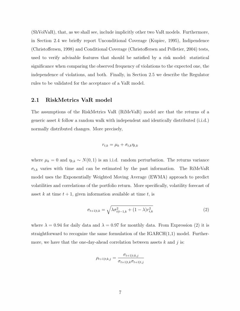
(ShVolVaR), that, as we shall see, include implicitly other two VaR models. Furthermore,

in Section 2.4 we briefly report Unconditional Coverage (Kupiec, 1995), Indipendence

(Christoffersen, 1998) and Conditional Coverage (Christoffersen and Pelletier, 2004) tests,

used to verify advisable features that should be satisfied by a risk model: statistical

significance when comparing the observed frequency of violations to the expected one, the

independence of violations, and both. Finally, in Section 2.5 we describe the Regulator

rules to be validated for the acceptance of a VaR model.

2.1 RiskMetrics VaR model

The assumptions of the RiskMetrics VaR (RiMeVaR) model are that the returns of a

generic asset k follow a random walk with independent and identically distributed (i.i.d.)

normally distributed changes. More precisely,

rt,k = µk + σt,kηt,k

where µk = 0 and ηt,k ∼ N(0, 1) is an i.i.d. random perturbation. The returns variance

σt,k varies with time and can be estimated by the past information. The RiMeVaR

model uses the Exponentially Weighted Moving Average (EWMA) approach to predict

volatilities and correlations of the portfolio return. More specifically, volatility forecast of

asset k at time t+ 1, given information available at time t, is

σt+1|t,k =√

λσ2t|t−1,k + (1− λ)r2t,k (2)

where λ = 0.94 for daily data and λ = 0.97 for monthly data. From Expression (2) it is

straightforward to recognize the same formulation of the IGARCH(1,1) model. Further-

more, we have that the one-day-ahead correlation between assets k and j is:

ρt+1|t;k,j =σt+1|t;k,j

σt+1|t,kσt+1|t,j

7

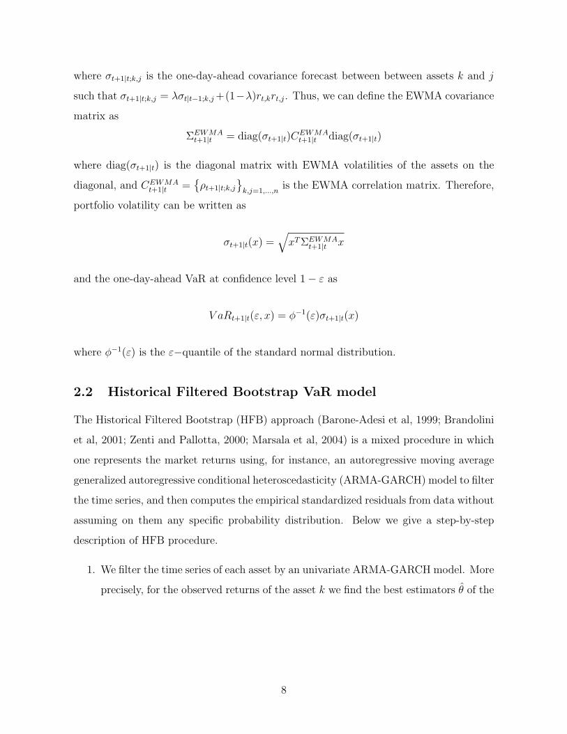
where σt+1|t;k,j is the one-day-ahead covariance forecast between between assets k and j

such that σt+1|t;k,j = λσt|t−1;k,j+(1−λ)rt,krt,j. Thus, we can define the EWMA covariance

matrix as

ΣEWMAt+1|t = diag(σt+1|t)C

EWMAt+1|t diag(σt+1|t)

where diag(σt+1|t) is the diagonal matrix with EWMA volatilities of the assets on the

diagonal, and CEWMAt+1|t =

{ρt+1|t;k,j

}k,j=1,...,n

is the EWMA correlation matrix. Therefore,

portfolio volatility can be written as

σt+1|t(x) =√

xTΣEWMAt+1|t x

and the one-day-ahead VaR at confidence level 1− ε as

V aRt+1|t(ε, x) = ϕ−1(ε)σt+1|t(x)

where ϕ−1(ε) is the ε−quantile of the standard normal distribution.

2.2 Historical Filtered Bootstrap VaR model

The Historical Filtered Bootstrap (HFB) approach (Barone-Adesi et al, 1999; Brandolini

et al, 2001; Zenti and Pallotta, 2000; Marsala et al, 2004) is a mixed procedure in which

one represents the market returns using, for instance, an autoregressive moving average

generalized autoregressive conditional heteroscedasticity (ARMA-GARCH) model to filter

the time series, and then computes the empirical standardized residuals from data without

assuming on them any specific probability distribution. Below we give a step-by-step

description of HFB procedure.

1. We filter the time series of each asset by an univariate ARMA-GARCH model. More

precisely, for the observed returns of the asset k we find the best estimators θ of the

8

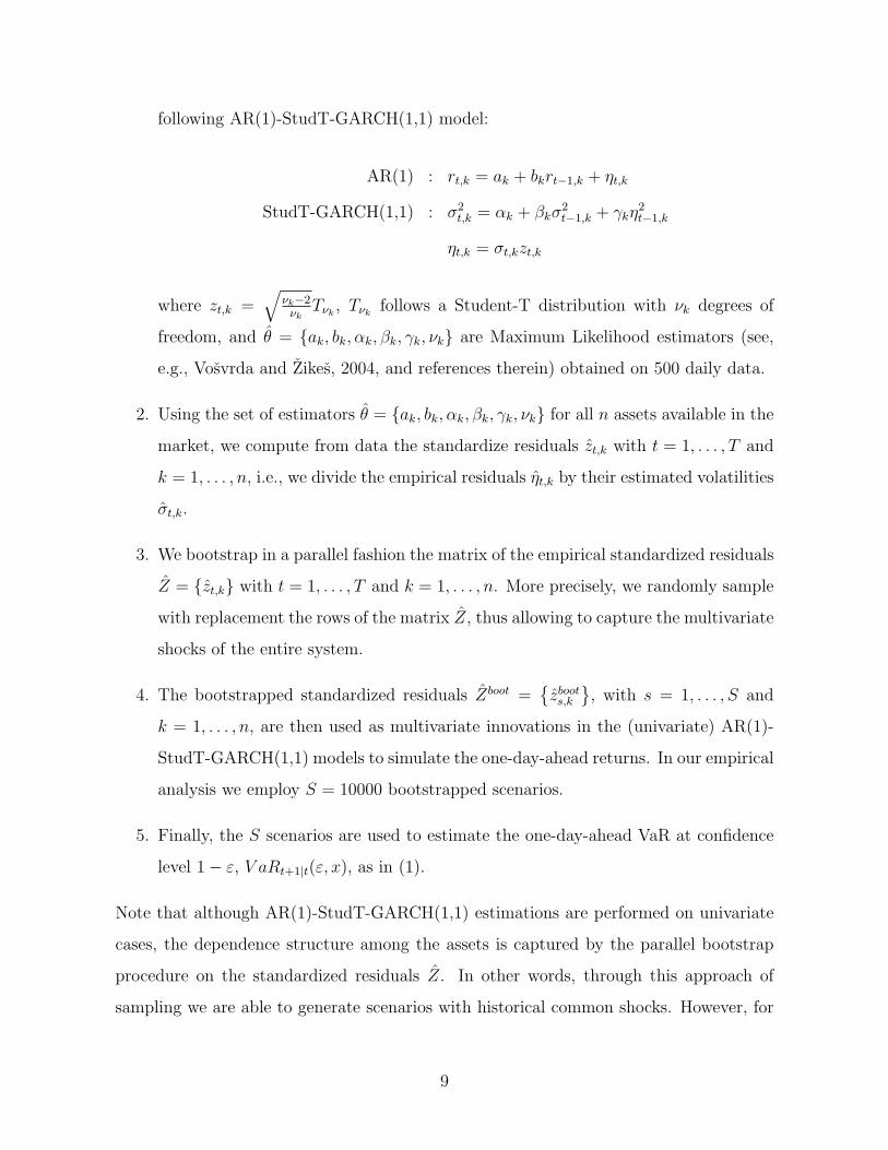
following AR(1)-StudT-GARCH(1,1) model:

AR(1) : rt,k = ak + bkrt−1,k + ηt,k

StudT-GARCH(1,1) : σ2t,k = αk + βkσ

2t−1,k + γkη

2t−1,k

ηt,k = σt,kzt,k

where zt,k =√

νk−2νk

Tνk , Tνk follows a Student-T distribution with νk degrees of

freedom, and θ = {ak, bk, αk, βk, γk, νk} are Maximum Likelihood estimators (see,

e.g., Vosvrda and Zikes, 2004, and references therein) obtained on 500 daily data.

2. Using the set of estimators θ = {ak, bk, αk, βk, γk, νk} for all n assets available in the

market, we compute from data the standardize residuals zt,k with t = 1, . . . , T and

k = 1, . . . , n, i.e., we divide the empirical residuals ηt,k by their estimated volatilities

σt,k.

3. We bootstrap in a parallel fashion the matrix of the empirical standardized residuals

Z = {zt,k} with t = 1, . . . , T and k = 1, . . . , n. More precisely, we randomly sample

with replacement the rows of the matrix Z, thus allowing to capture the multivariate

shocks of the entire system.

4. The bootstrapped standardized residuals Zboot ={zboots,k

}, with s = 1, . . . , S and

k = 1, . . . , n, are then used as multivariate innovations in the (univariate) AR(1)-

StudT-GARCH(1,1) models to simulate the one-day-ahead returns. In our empirical

analysis we employ S = 10000 bootstrapped scenarios.

5. Finally, the S scenarios are used to estimate the one-day-ahead VaR at confidence

level 1− ε, V aRt+1|t(ε, x), as in (1).

Note that although AR(1)-StudT-GARCH(1,1) estimations are performed on univariate

cases, the dependence structure among the assets is captured by the parallel bootstrap

procedure on the standardized residuals Z. In other words, through this approach of

sampling we are able to generate scenarios with historical common shocks. However, for

9

more details see Barone-Adesi et al (1999); Brandolini et al (2001); Zenti and Pallotta

(2000); Marsala et al (2004).

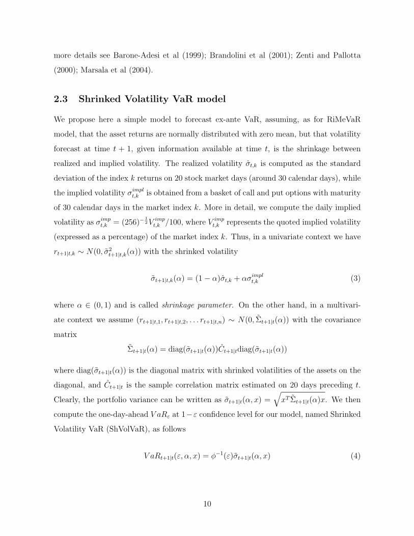
2.3 Shrinked Volatility VaR model

We propose here a simple model to forecast ex-ante VaR, assuming, as for RiMeVaR

model, that the asset returns are normally distributed with zero mean, but that volatility

forecast at time t + 1, given information available at time t, is the shrinkage between

realized and implied volatility. The realized volatility σt,k is computed as the standard

deviation of the index k returns on 20 stock market days (around 30 calendar days), while

the implied volatility σimplt,k is obtained from a basket of call and put options with maturity

of 30 calendar days in the market index k. More in detail, we compute the daily implied

volatility as σimpt,k = (256)−

12V imp

t,k /100, where V impt,k represents the quoted implied volatility

(expressed as a percentage) of the market index k. Thus, in a univariate context we have

rt+1|t,k ∼ N(0, σ2t+1|t,k(α)) with the shrinked volatility

σt+1|t,k(α) = (1− α)σt,k + ασimplt,k (3)

where α ∈ (0, 1) and is called shrinkage parameter. On the other hand, in a multivari-

ate context we assume (rt+1|t,1, rt+1|t,2, . . . rt+1|t,n) ∼ N(0, Σt+1|t(α)) with the covariance

matrix

Σt+1|t(α) = diag(σt+1|t(α))Ct+1|tdiag(σt+1|t(α))

where diag(σt+1|t(α)) is the diagonal matrix with shrinked volatilities of the assets on the

diagonal, and Ct+1|t is the sample correlation matrix estimated on 20 days preceding t.

Clearly, the portfolio variance can be written as σt+1|t(α, x) =√

xT Σt+1|t(α)x. We then

compute the one-day-ahead V aRε at 1−ε confidence level for our model, named Shrinked

Volatility VaR (ShVolVaR), as follows

V aRt+1|t(ε, α, x) = ϕ−1(ε)σt+1|t(α, x) (4)

10

In our empirical analysis we consider the shrinkage parameter α for different equally-

spaced values belonging to the interval (0, 1). Note that if α = 0, then Model (4) coincides

with the Realized Volatility VaR (ReVolVaR) model; while if α = 1 we have the Implied

Volatility VaR (ImVolVaR) model.

In Section 3 we will test and compare the ReVolVaR, ImVolVaR and ShVolVaR mod-

els with the Historical Filtered Bootstrap VaR (HFBVaR) and the RiskMetrics VaR

(RiMeVaR) models that are considered as benchmarks.

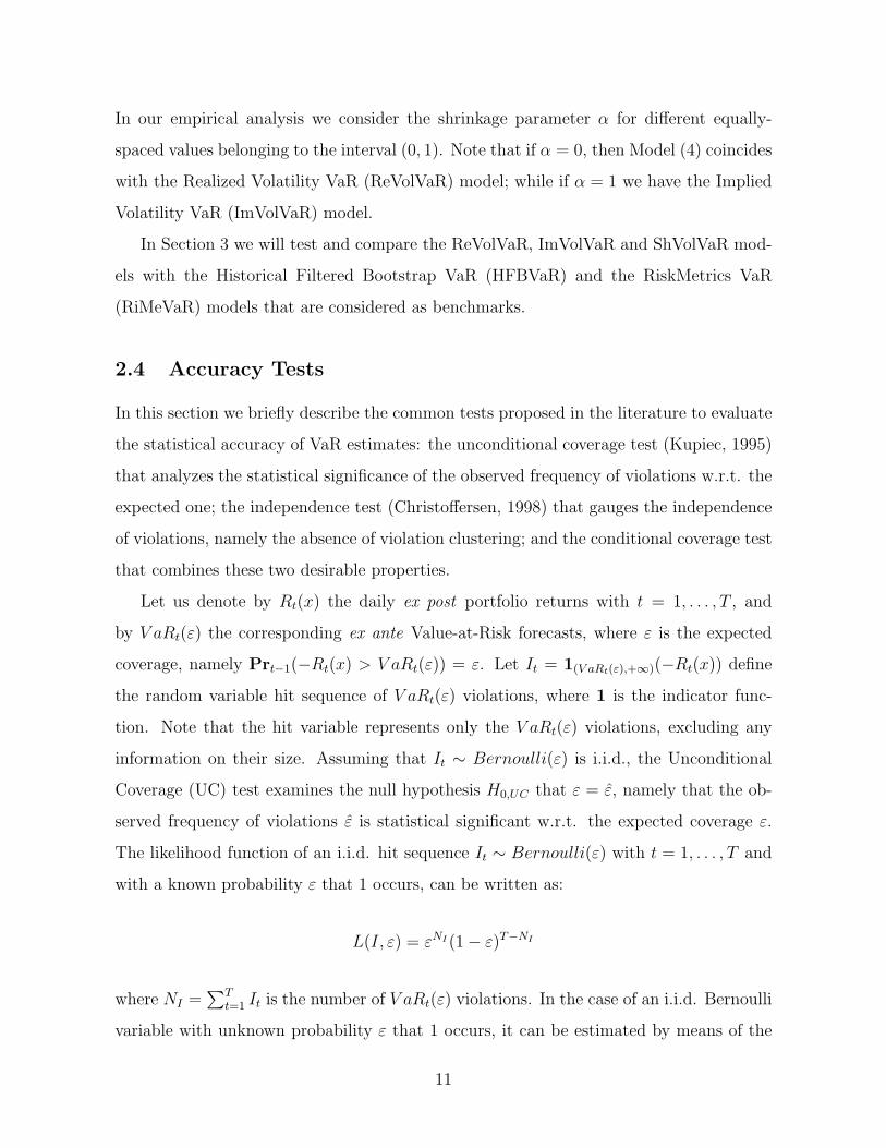
2.4 Accuracy Tests

In this section we briefly describe the common tests proposed in the literature to evaluate

the statistical accuracy of VaR estimates: the unconditional coverage test (Kupiec, 1995)

that analyzes the statistical significance of the observed frequency of violations w.r.t. the

expected one; the independence test (Christoffersen, 1998) that gauges the independence

of violations, namely the absence of violation clustering; and the conditional coverage test

that combines these two desirable properties.

Let us denote by Rt(x) the daily ex post portfolio returns with t = 1, . . . , T , and

by V aRt(ε) the corresponding ex ante Value-at-Risk forecasts, where ε is the expected

coverage, namely Prt−1(−Rt(x) > V aRt(ε)) = ε. Let It = 1(V aRt(ε),+∞)(−Rt(x)) define

the random variable hit sequence of V aRt(ε) violations, where 1 is the indicator func-

tion. Note that the hit variable represents only the V aRt(ε) violations, excluding any

information on their size. Assuming that It ∼ Bernoulli(ε) is i.i.d., the Unconditional

Coverage (UC) test examines the null hypothesis H0,UC that ε = ε, namely that the ob-

served frequency of violations ε is statistical significant w.r.t. the expected coverage ε.

The likelihood function of an i.i.d. hit sequence It ∼ Bernoulli(ε) with t = 1, . . . , T and

with a known probability ε that 1 occurs, can be written as:

L(I, ε) = εNI (1− ε)T−NI

where NI =∑T

t=1 It is the number of V aRt(ε) violations. In the case of an i.i.d. Bernoulli

variable with unknown probability ε that 1 occurs, it can be estimated by means of the

11

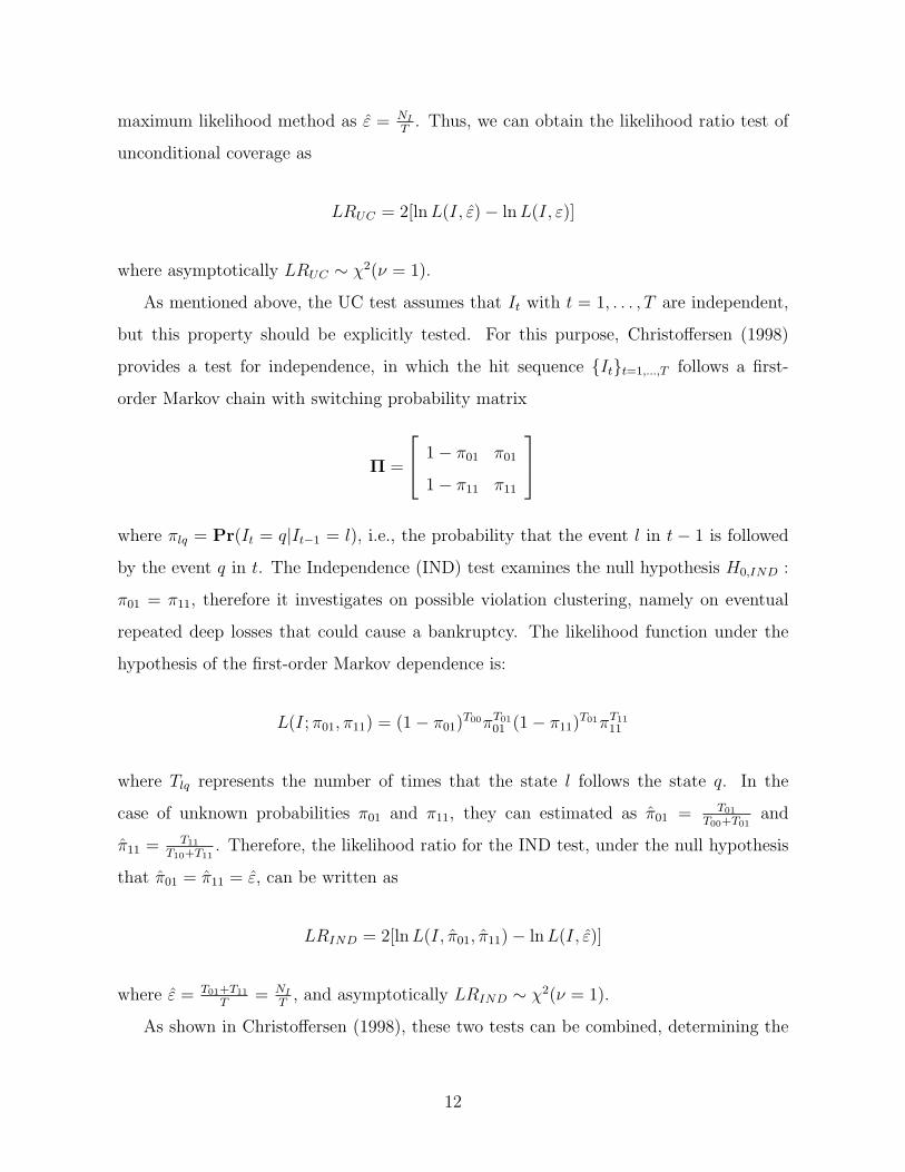
maximum likelihood method as ε = NI

T. Thus, we can obtain the likelihood ratio test of

unconditional coverage as

LRUC = 2[lnL(I, ε)− lnL(I, ε)]

where asymptotically LRUC ∼ χ2(ν = 1).

As mentioned above, the UC test assumes that It with t = 1, . . . , T are independent,

but this property should be explicitly tested. For this purpose, Christoffersen (1998)

provides a test for independence, in which the hit sequence {It}t=1,...,T follows a first-

order Markov chain with switching probability matrix

Π =

1− π01 π01

1− π11 π11

where πlq = Pr(It = q|It−1 = l), i.e., the probability that the event l in t − 1 is followed

by the event q in t. The Independence (IND) test examines the null hypothesis H0,IND :

π01 = π11, therefore it investigates on possible violation clustering, namely on eventual

repeated deep losses that could cause a bankruptcy. The likelihood function under the

hypothesis of the first-order Markov dependence is:

L(I;π01, π11) = (1− π01)T00πT01

01 (1− π11)T01πT11

11

where Tlq represents the number of times that the state l follows the state q. In the

case of unknown probabilities π01 and π11, they can estimated as π01 = T01

T00+T01and

π11 =T11

T10+T11. Therefore, the likelihood ratio for the IND test, under the null hypothesis

that π01 = π11 = ε, can be written as

LRIND = 2[lnL(I, π01, π11)− lnL(I, ε)]

where ε = T01+T11

T= NI

T, and asymptotically LRIND ∼ χ2(ν = 1).

As shown in Christoffersen (1998), these two tests can be combined, determining the

12

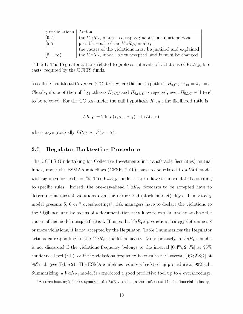
♯ of violations Action[0, 4] the V aR1% model is accepted; no actions must be done[5, 7] possible crash of the V aR1% model;

the causes of the violations must be justified and explained[8,+∞) the V aR1% model is not accepted, and it must be changed

Table 1: The Regulator actions related to prefixed intervals of violations of V aR1% fore-casts, required by the UCITS funds.

so-called Conditional Coverage (CC) test, where the null hypothesisH0,CC : π01 = π11 = ε.

Clearly, if one of the null hypotheses H0,UC and H0,IND is rejected, even H0,CC will tend

to be rejected. For the CC test under the null hypothesis H0,CC , the likelihood ratio is

LRCC = 2[lnL(I, π01, π11)− lnL(I, ε)]

where asymptotically LRCC ∼ χ2(ν = 2).

2.5 Regulator Backtesting Procedure

The UCITS (Undertaking for Collective Investments in Transferable Securities) mutual

funds, under the ESMA’s guidelines (CESR, 2010), have to be related to a VaR model

with significance level ε =1%. This V aR1% model, in turn, have to be validated according

to specific rules. Indeed, the one-day-ahead V aR1% forecasts to be accepted have to

determine at most 4 violations over the earlier 250 (stock market) days. If a V aR1%

model presents 5, 6 or 7 overshootings1, risk managers have to declare the violations to

the Vigilance, and by means of a documentation they have to explain and to analyze the

causes of the model misspecification. If instead a V aR1% prediction strategy determines 8

or more violations, it is not accepted by the Regulator. Table 1 summarizes the Regulator

actions corresponding to the V aR1% model behavior. More precisely, a V aR1% model

is not discarded if the violations frequency belongs to the interval [0.4%; 2.4%] at 95%

confidence level (c.l.), or if the violations frequency belongs to the interval [0%; 2.8%] at

99% c.l. (see Table 2). The ESMA guidelines require a backtesting procedure at 99% c.l..

Summarizing, a V aR1% model is considered a good predictive tool up to 4 overshootings,

1An overshooting is here a synonym of a VaR violation, a word often used in the financial industry.

13

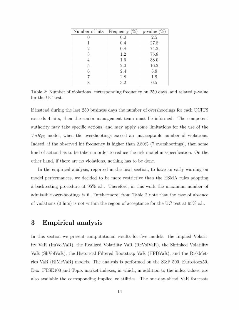
Number of hits Frequency (%) p-value (%)0 0.0 2.51 0.4 27.82 0.8 74.23 1.2 75.84 1.6 38.05 2.0 16.26 2.4 5.97 2.8 1.98 3.2 0.5

Table 2: Number of violations, corresponding frequency on 250 days, and related p-valuefor the UC test.

if instead during the last 250 business days the number of overshootings for each UCITS

exceeds 4 hits, then the senior management team must be informed. The competent

authority may take specific actions, and may apply some limitations for the use of the

V aR1% model, when the overshootings exceed an unacceptable number of violations.

Indeed, if the observed hit frequency is higher than 2.80% (7 overshootings), then some

kind of action has to be taken in order to reduce the risk model misspecification. On the

other hand, if there are no violations, nothing has to be done.

In the empirical analysis, reported in the next section, to have an early warning on

model performances, we decided to be more restrictive than the ESMA rules adopting

a backtesting procedure at 95% c.l.. Therefore, in this work the maximum number of

admissible overshootings is 6. Furthermore, from Table 2 note that the case of absence

of violations (0 hits) is not within the region of acceptance for the UC test at 95% c.l..

3 Empirical analysis

In this section we present computational results for five models: the Implied Volatil-

ity VaR (ImVolVaR), the Realized Volatility VaR (ReVolVaR), the Shrinked Volatility

VaR (ShVolVaR), the Historical Filtered Bootstrap VaR (HFBVaR), and the RiskMet-

rics VaR (RiMeVaR) models. The analysis is performed on the S&P 500, Eurostoxx50,

Dax, FTSE100 and Topix market indexes, in which, in addition to the index values, are

also available the corresponding implied volatilities. The one-day-ahead VaR forecasts

14

Market Index Implied Volatility Start End daily VaRticker ticker date date forecasts

SP500 SPTR VIX 30/01/1990 30/9/2015 6472Eurostoxx50 SX5T V2X 01/02/1999 30/9/2015 4265

DAX DAX V1X 30/01/1992 30/9/2015 5994FTSE100 TUKXG VFTSE 01/02/2000 30/9/2015 3959Topix TPXDDVD VXJ 02/03/1998 30/9/2015 4320

Table 3: List of the data sets analyzed.

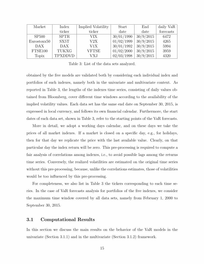
obtained by the five models are validated both by considering each individual index and

portfolios of such indexes, namely both in the univariate and multivariate context. As

reported in Table 3, the lengths of the indexes time series, consisting of daily values ob-

tained from Bloomberg, cover different time windows according to the availability of the

implied volatility values. Each data set has the same end date on September 30, 2015, is

expressed in local currency, and follows its own financial calendar. Furthermore, the start

dates of each data set, shown in Table 3, refer to the starting points of the VaR forecasts.

More in detail, we adopt a working days calendar, and on these days we take the

prices of all market indexes. If a market is closed on a specific day, e.g., for holidays,

then for that day we replicate the price with the last available value. Clearly, on that

particular day the index return will be zero. This pre-processing is required to compute a

fair analysis of correlations among indexes, i.e., to avoid possible lags among the returns

time series. Conversely, the realized volatilities are estimated on the original time series

without this pre-processing, because, unlike the correlations estimates, those of volatilities

would be too influenced by this pre-processing.

For completeness, we also list in Table 3 the tickers corresponding to each time se-

ries. In the case of VaR forecasts analysis for portfolios of the five indexes, we consider

the maximum time window covered by all data sets, namely from February 1, 2000 to

September 30, 2015.

3.1 Computational Results

In this section we discuss the main results on the behavior of the VaR models in the

univariate (Section 3.1.1) and in the multivariate (Section 3.1.2) framework.

15

3.1.1 Univariate framework

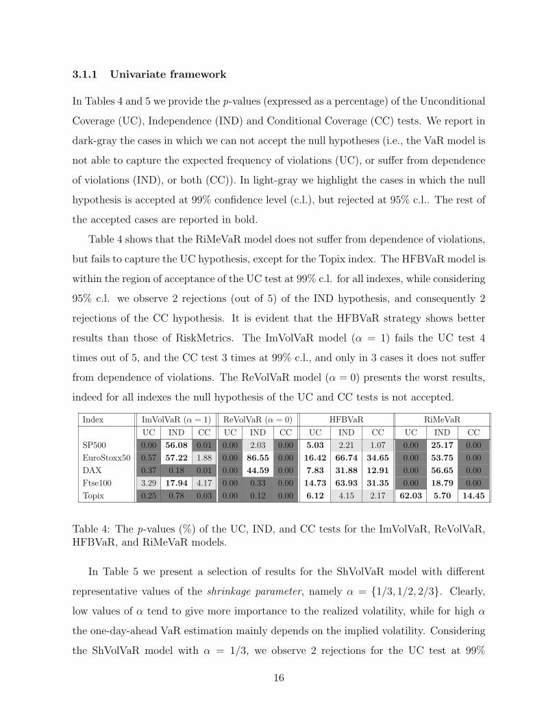
In Tables 4 and 5 we provide the p-values (expressed as a percentage) of the Unconditional

Coverage (UC), Independence (IND) and Conditional Coverage (CC) tests. We report in

dark-gray the cases in which we can not accept the null hypotheses (i.e., the VaR model is

not able to capture the expected frequency of violations (UC), or suffer from dependence

of violations (IND), or both (CC)). In light-gray we highlight the cases in which the null

hypothesis is accepted at 99% confidence level (c.l.), but rejected at 95% c.l.. The rest of

the accepted cases are reported in bold.

Table 4 shows that the RiMeVaR model does not suffer from dependence of violations,

but fails to capture the UC hypothesis, except for the Topix index. The HFBVaR model is

within the region of acceptance of the UC test at 99% c.l. for all indexes, while considering

95% c.l. we observe 2 rejections (out of 5) of the IND hypothesis, and consequently 2

rejections of the CC hypothesis. It is evident that the HFBVaR strategy shows better

results than those of RiskMetrics. The ImVolVaR model (α = 1) fails the UC test 4

times out of 5, and the CC test 3 times at 99% c.l., and only in 3 cases it does not suffer

from dependence of violations. The ReVolVaR model (α = 0) presents the worst results,

indeed for all indexes the null hypothesis of the UC and CC tests is not accepted.

Index ImVolVaR (α = 1) ReVolVaR (α = 0) HFBVaR RiMeVaR

UC IND CC UC IND CC UC IND CC UC IND CC

SP500 0.00 56.08 0.01 0.00 2.03 0.00 5.03 2.21 1.07 0.00 25.17 0.00

EuroStoxx50 0.57 57.22 1.88 0.00 86.55 0.00 16.42 66.74 34.65 0.00 53.75 0.00

DAX 0.37 0.18 0.01 0.00 44.59 0.00 7.83 31.88 12.91 0.00 56.65 0.00

Ftse100 3.29 17.94 4.17 0.00 0.33 0.00 14.73 63.93 31.35 0.00 18.79 0.00

Topix 0.25 0.78 0.03 0.00 0.12 0.00 6.12 4.15 2.17 62.03 5.70 14.45

Table 4: The p-values (%) of the UC, IND, and CC tests for the ImVolVaR, ReVolVaR,HFBVaR, and RiMeVaR models.

In Table 5 we present a selection of results for the ShVolVaR model with different

representative values of the shrinkage parameter, namely α = {1/3, 1/2, 2/3}. Clearly,

low values of α tend to give more importance to the realized volatility, while for high α

the one-day-ahead VaR estimation mainly depends on the implied volatility. Considering

the ShVolVaR model with α = 1/3, we observe 2 rejections for the UC test at 99%

16

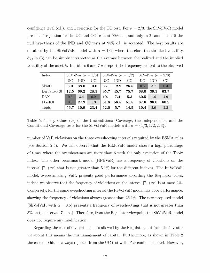
confidence level (c.l.), and 1 rejection for the CC test. For α = 2/3, the ShVolVaR model

presents 1 rejection for the UC and CC tests at 99% c.l., and only in 2 cases out of 5 the

null hypothesis of the IND and CC tests at 95% c.l. is accepted. The best results are

obtained by the ShVolVaR model with α = 1/2, where therefore the shrinked volatility

σk,t in (3) can be simply interpreted as the average between the realized and the implied

volatility of the asset k. In Tables 6 and 7 we report the frequency related to the observed

Index ShVolVar (α = 1/3) ShVolVar (α = 1/2) ShVolVar (α = 2/3)

UC IND CC UC IND CC UC IND CC

SP500 5.0 38.0 10.0 55.1 12.9 26.5 0.6 3.7 0.3

EuroStoxx50 12.5 69.2 28.5 95.7 45.7 75.7 68.0 39.3 63.7

DAX 0.5 3.4 0.2 10.1 7.4 5.3 60.5 1.6 4.9

Ftse100 0.6 27.9 1.3 31.8 56.5 51.5 67.6 36.0 60.2

Topix 56.7 10.9 23.4 62.0 5.7 14.5 10.4 2.6 2.2

Table 5: The p-values (%) of the Unconditional Coverage, the Independence, and theConditional Coverage tests for the ShVolVaR models with α = {1/3, 1/2, 2/3}.

number of VaR violations on the three overshooting intervals required by the ESMA rules

(see Section 2.5). We can observe that the RiMeVaR model shows a high percentage

of times where the overshootings are more than 6 with the only exception of the Topix

index. The other benchmark model (HFBVaR) has a frequency of violations on the

interval [7,+∞) that is not greater than 5.1% for the different indexes. The ImVolVaR

model, overestimating VaR, presents good performance according the Regulator rules,

indeed we observe that the frequency of violations on the interval [7,+∞) is at most 2%.

Conversely, for the same overshooting interval the ReVolVaR model has poor performance,

showing the frequency of violations always greater than 26.1%. The new proposed model

(ShVolVaR with α = 0.5) presents a frequency of overshootings that is not greater than

3% on the interval [7,+∞). Therefore, from the Regulator viewpoint the ShVolVaR model

does not require any modification.

Regarding the case of 0 violations, it is allowed by the Regulator, but from the investor

viewpoint this means the mismanagement of capital. Furthermore, as shown in Table 2

the case of 0 hits is always rejected from the UC test with 95% confidence level. However,

17

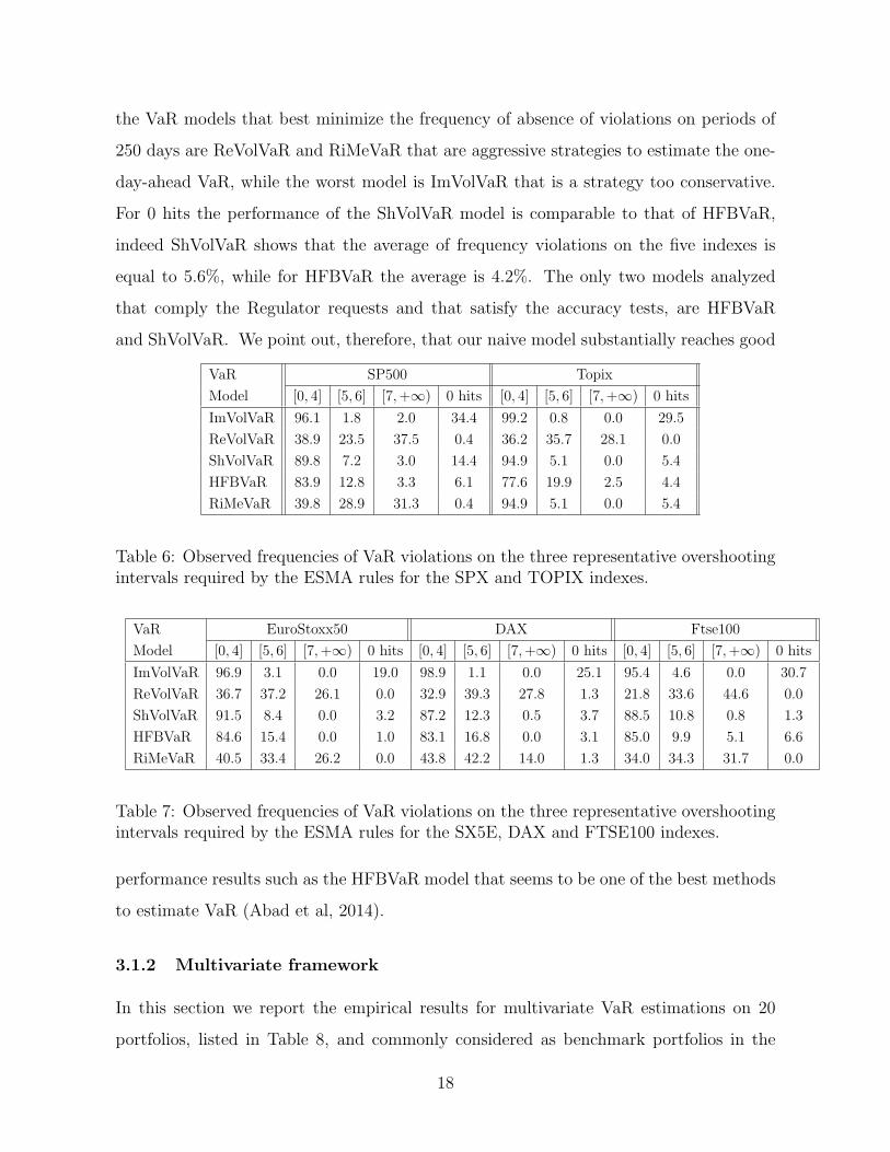
the VaR models that best minimize the frequency of absence of violations on periods of

250 days are ReVolVaR and RiMeVaR that are aggressive strategies to estimate the one-

day-ahead VaR, while the worst model is ImVolVaR that is a strategy too conservative.

For 0 hits the performance of the ShVolVaR model is comparable to that of HFBVaR,

indeed ShVolVaR shows that the average of frequency violations on the five indexes is

equal to 5.6%, while for HFBVaR the average is 4.2%. The only two models analyzed

that comply the Regulator requests and that satisfy the accuracy tests, are HFBVaR

and ShVolVaR. We point out, therefore, that our naive model substantially reaches good

VaR SP500 Topix

Model [0, 4] [5, 6] [7,+∞) 0 hits [0, 4] [5, 6] [7,+∞) 0 hits

ImVolVaR 96.1 1.8 2.0 34.4 99.2 0.8 0.0 29.5

ReVolVaR 38.9 23.5 37.5 0.4 36.2 35.7 28.1 0.0

ShVolVaR 89.8 7.2 3.0 14.4 94.9 5.1 0.0 5.4

HFBVaR 83.9 12.8 3.3 6.1 77.6 19.9 2.5 4.4

RiMeVaR 39.8 28.9 31.3 0.4 94.9 5.1 0.0 5.4

Table 6: Observed frequencies of VaR violations on the three representative overshootingintervals required by the ESMA rules for the SPX and TOPIX indexes.

VaR EuroStoxx50 DAX Ftse100

Model [0, 4] [5, 6] [7,+∞) 0 hits [0, 4] [5, 6] [7,+∞) 0 hits [0, 4] [5, 6] [7,+∞) 0 hits

ImVolVaR 96.9 3.1 0.0 19.0 98.9 1.1 0.0 25.1 95.4 4.6 0.0 30.7

ReVolVaR 36.7 37.2 26.1 0.0 32.9 39.3 27.8 1.3 21.8 33.6 44.6 0.0

ShVolVaR 91.5 8.4 0.0 3.2 87.2 12.3 0.5 3.7 88.5 10.8 0.8 1.3

HFBVaR 84.6 15.4 0.0 1.0 83.1 16.8 0.0 3.1 85.0 9.9 5.1 6.6

RiMeVaR 40.5 33.4 26.2 0.0 43.8 42.2 14.0 1.3 34.0 34.3 31.7 0.0

Table 7: Observed frequencies of VaR violations on the three representative overshootingintervals required by the ESMA rules for the SX5E, DAX and FTSE100 indexes.

performance results such as the HFBVaR model that seems to be one of the best methods

to estimate VaR (Abad et al, 2014).

3.1.2 Multivariate framework

In this section we report the empirical results for multivariate VaR estimations on 20

portfolios, listed in Table 8, and commonly considered as benchmark portfolios in the

18

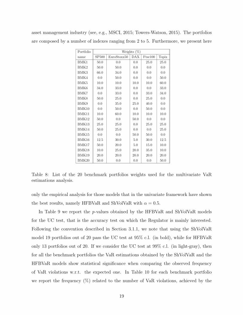
asset management industry (see, e.g., MSCI, 2015; Towers-Watson, 2015). The portfolios

are composed by a number of indexes ranging from 2 to 5. Furthermore, we present here

Portfolio Weights (%)

name SP500 EuroStoxx50 DAX Ftse100 Topix

BMK1 50.0 0.0 0.0 25.0 25.0

BMK2 50.0 50.0 0.0 0.0 0.0

BMK3 66.0 34.0 0.0 0.0 0.0

BMK4 0.0 50.0 0.0 0.0 50.0

BMK5 10.0 10.0 10.0 10.0 60.0

BMK6 34.0 33.0 0.0 0.0 33.0

BMK7 0.0 33.0 0.0 33.0 34.0

BMK8 50.0 25.0 0.0 25.0 0.0

BMK9 0.0 35.0 25.0 40.0 0.0

BMK10 0.0 50.0 0.0 50.0 0.0

BMK11 10.0 60.0 10.0 10.0 10.0

BMK12 50.0 0.0 50.0 0.0 0.0

BMK13 25.0 25.0 0.0 25.0 25.0

BMK14 50.0 25.0 0.0 0.0 25.0

BMK15 0.0 0.0 50.0 50.0 0.0

BMK16 12.5 30.0 5.0 30.0 12.5

BMK17 50.0 20.0 5.0 15.0 10.0

BMK18 10.0 25.0 20.0 35.0 10.0

BMK19 20.0 20.0 20.0 20.0 20.0

BMK20 50.0 0.0 0.0 0.0 50.0

Table 8: List of the 20 benchmark portfolios weights used for the multivariate VaRestimations analysis.

only the empirical analysis for those models that in the univariate framework have shown

the best results, namely HFBVaR and ShVolVaR with α = 0.5.

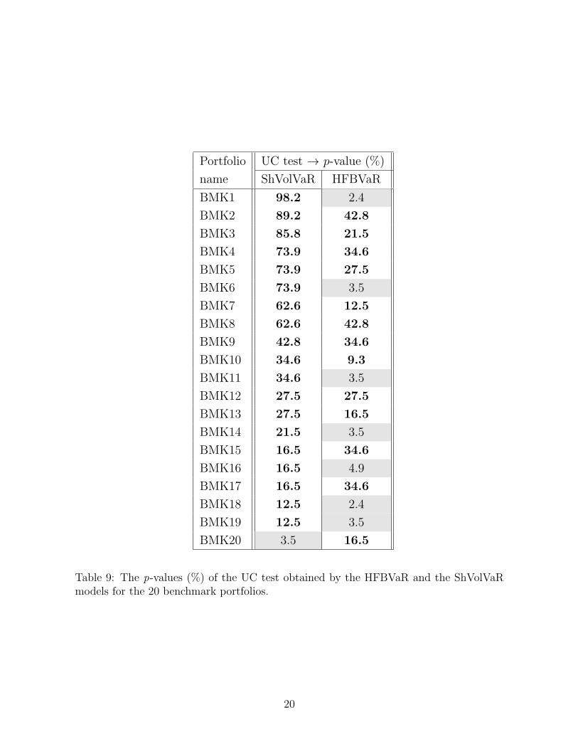
In Table 9 we report the p-values obtained by the HFBVaR and ShVolVaR models

for the UC test, that is the accuracy test on which the Regulator is mainly interested.

Following the convention described in Section 3.1.1, we note that using the ShVolVaR

model 19 portfolios out of 20 pass the UC test at 95% c.l. (in bold), while for HFBVaR

only 13 portfolios out of 20. If we consider the UC test at 99% c.l. (in light-gray), then

for all the benchmark portfolios the VaR estimations obtained by the ShVolVaR and the

HFBVaR models show statistical significance when comparing the observed frequency

of VaR violations w.r.t. the expected one. In Table 10 for each benchmark portfolio

we report the frequency (%) related to the number of VaR violations, achieved by the

19

Portfolio UC test → p-value (%)

name ShVolVaR HFBVaR

BMK1 98.2 2.4

BMK2 89.2 42.8

BMK3 85.8 21.5

BMK4 73.9 34.6

BMK5 73.9 27.5

BMK6 73.9 3.5

BMK7 62.6 12.5

BMK8 62.6 42.8

BMK9 42.8 34.6

BMK10 34.6 9.3

BMK11 34.6 3.5

BMK12 27.5 27.5

BMK13 27.5 16.5

BMK14 21.5 3.5

BMK15 16.5 34.6

BMK16 16.5 4.9

BMK17 16.5 34.6

BMK18 12.5 2.4

BMK19 12.5 3.5

BMK20 3.5 16.5

Table 9: The p-values (%) of the UC test obtained by the HFBVaR and the ShVolVaRmodels for the 20 benchmark portfolios.

20

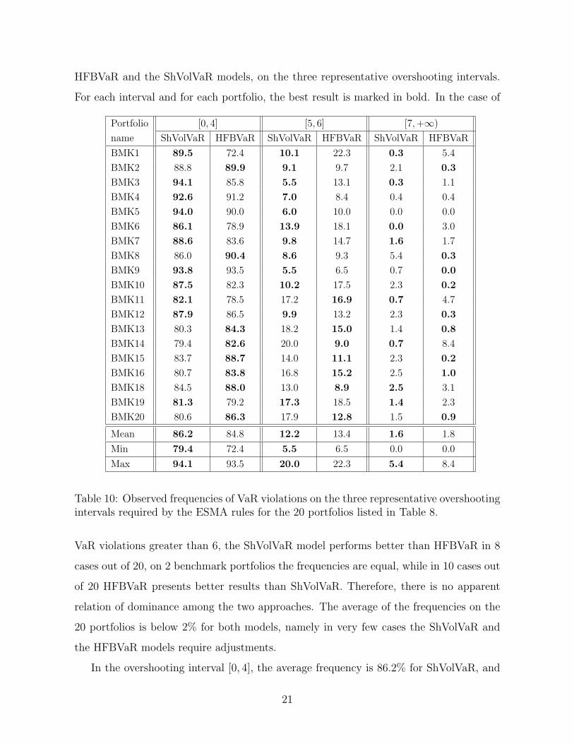
HFBVaR and the ShVolVaR models, on the three representative overshooting intervals.

For each interval and for each portfolio, the best result is marked in bold. In the case of

Portfolio [0, 4] [5, 6] [7,+∞)

name ShVolVaR HFBVaR ShVolVaR HFBVaR ShVolVaR HFBVaR

BMK1 89.5 72.4 10.1 22.3 0.3 5.4

BMK2 88.8 89.9 9.1 9.7 2.1 0.3

BMK3 94.1 85.8 5.5 13.1 0.3 1.1

BMK4 92.6 91.2 7.0 8.4 0.4 0.4

BMK5 94.0 90.0 6.0 10.0 0.0 0.0

BMK6 86.1 78.9 13.9 18.1 0.0 3.0

BMK7 88.6 83.6 9.8 14.7 1.6 1.7

BMK8 86.0 90.4 8.6 9.3 5.4 0.3

BMK9 93.8 93.5 5.5 6.5 0.7 0.0

BMK10 87.5 82.3 10.2 17.5 2.3 0.2

BMK11 82.1 78.5 17.2 16.9 0.7 4.7

BMK12 87.9 86.5 9.9 13.2 2.3 0.3

BMK13 80.3 84.3 18.2 15.0 1.4 0.8

BMK14 79.4 82.6 20.0 9.0 0.7 8.4

BMK15 83.7 88.7 14.0 11.1 2.3 0.2

BMK16 80.7 83.8 16.8 15.2 2.5 1.0

BMK18 84.5 88.0 13.0 8.9 2.5 3.1

BMK19 81.3 79.2 17.3 18.5 1.4 2.3

BMK20 80.6 86.3 17.9 12.8 1.5 0.9

Mean 86.2 84.8 12.2 13.4 1.6 1.8

Min 79.4 72.4 5.5 6.5 0.0 0.0

Max 94.1 93.5 20.0 22.3 5.4 8.4

Table 10: Observed frequencies of VaR violations on the three representative overshootingintervals required by the ESMA rules for the 20 portfolios listed in Table 8.

VaR violations greater than 6, the ShVolVaR model performs better than HFBVaR in 8

cases out of 20, on 2 benchmark portfolios the frequencies are equal, while in 10 cases out

of 20 HFBVaR presents better results than ShVolVaR. Therefore, there is no apparent

relation of dominance among the two approaches. The average of the frequencies on the

20 portfolios is below 2% for both models, namely in very few cases the ShVolVaR and

the HFBVaR models require adjustments.

In the overshooting interval [0, 4], the average frequency is 86.2% for ShVolVaR, and

21

84.8% for HFBVaR. For the intermediate interval [5, 6] the ShVolVaR and the HFBVaR

models show average frequencies of 12.2% and of 13.4%, respectively. Thus even in these

cases the two approaches seems to have similar performance.

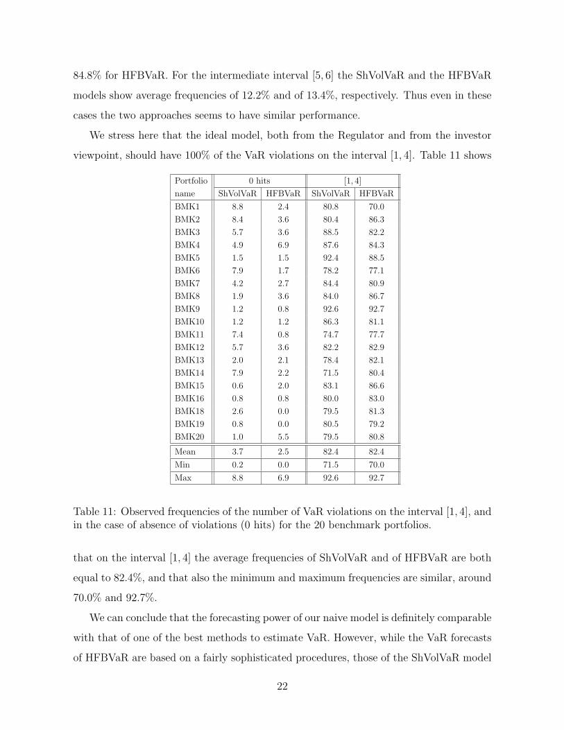
We stress here that the ideal model, both from the Regulator and from the investor

viewpoint, should have 100% of the VaR violations on the interval [1, 4]. Table 11 shows

Portfolio 0 hits [1, 4]

name ShVolVaR HFBVaR ShVolVaR HFBVaR

BMK1 8.8 2.4 80.8 70.0

BMK2 8.4 3.6 80.4 86.3

BMK3 5.7 3.6 88.5 82.2

BMK4 4.9 6.9 87.6 84.3

BMK5 1.5 1.5 92.4 88.5

BMK6 7.9 1.7 78.2 77.1

BMK7 4.2 2.7 84.4 80.9

BMK8 1.9 3.6 84.0 86.7

BMK9 1.2 0.8 92.6 92.7

BMK10 1.2 1.2 86.3 81.1

BMK11 7.4 0.8 74.7 77.7

BMK12 5.7 3.6 82.2 82.9

BMK13 2.0 2.1 78.4 82.1

BMK14 7.9 2.2 71.5 80.4

BMK15 0.6 2.0 83.1 86.6

BMK16 0.8 0.8 80.0 83.0

BMK18 2.6 0.0 79.5 81.3

BMK19 0.8 0.0 80.5 79.2

BMK20 1.0 5.5 79.5 80.8

Mean 3.7 2.5 82.4 82.4

Min 0.2 0.0 71.5 70.0

Max 8.8 6.9 92.6 92.7

Table 11: Observed frequencies of the number of VaR violations on the interval [1, 4], andin the case of absence of violations (0 hits) for the 20 benchmark portfolios.

that on the interval [1, 4] the average frequencies of ShVolVaR and of HFBVaR are both

equal to 82.4%, and that also the minimum and maximum frequencies are similar, around

70.0% and 92.7%.

We can conclude that the forecasting power of our naive model is definitely comparable

with that of one of the best methods to estimate VaR. However, while the VaR forecasts

of HFBVaR are based on a fairly sophisticated procedures, those of the ShVolVaR model

22

are extremely simple to obtain.

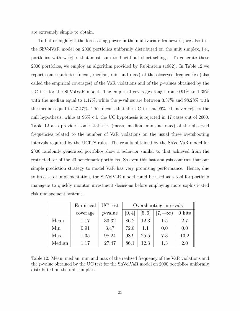
To better highlight the forecasting power in the multivariate framework, we also test

the ShVolVaR model on 2000 portfolios uniformly distributed on the unit simplex, i.e.,

portfolios with weights that must sum to 1 without short-sellings. To generate these

2000 portfolios, we employ an algorithm provided by Rubinstein (1982). In Table 12 we

report some statistics (mean, median, min and max) of the observed frequencies (also

called the empirical coverages) of the VaR violations and of the p-values obtained by the

UC test for the ShVolVaR model. The empirical coverages range from 0.91% to 1.35%

with the median equal to 1.17%, while the p-values are between 3.37% and 98.28% with

the median equal to 27.47%. This means that the UC test at 99% c.l. never rejects the

null hypothesis, while at 95% c.l. the UC hypothesis is rejected in 17 cases out of 2000.

Table 12 also provides some statistics (mean, median, min and max) of the observed

frequencies related to the number of VaR violations on the usual three overshooting

intervals required by the UCITS rules. The results obtained by the ShVolVaR model for

2000 randomly generated portfolios show a behavior similar to that achieved from the

restricted set of the 20 benchmark portfolios. So even this last analysis confirms that our

simple prediction strategy to model VaR has very promising performance. Hence, due

to its ease of implementation, the ShVolVaR model could be used as a tool for portfolio

managers to quickly monitor investment decisions before employing more sophisticated

risk management systems.

Empirical UC test Overshooting intervals

coverage p-value [0, 4] [5, 6] [7,+∞) 0 hits

Mean 1.17 33.32 86.2 12.3 1.5 2.7

Min 0.91 3.47 72.8 1.1 0.0 0.0

Max 1.35 98.24 98.9 25.5 7.3 13.2

Median 1.17 27.47 86.1 12.3 1.3 2.0

Table 12: Mean, median, min and max of the realized frequency of the VaR violations andthe p-value obtained by the UC test for the ShVolVaR model on 2000 portfolios uniformlydistributed on the unit simplex.

23

4 Conclusions

In this work we proposed a new method to predict VaR, both using variables known on

the market (implied volatilities) and variable estimated on data (realized volatilities). The

main idea behind our approach is to use a combination of information both on the ex-

pected future risk and on the past estimated risk. The forecasting power of our ShVolVaR

model is compared with that of several models proposed in the literature, including one

of the best methods to estimate VaR, such as the HFBVaR model. All models are tested

both on the statistical accuracy (by means of the Unconditional Coverage, the Indepen-

dence and the Conditional Coverage tests) and on efficiency (by means of the backtesting

procedure of the Vigilance). Furthermore, they are validated both on individual asset and

on portfolios of such assets, namely both in the univariate and multivariate framework.

Although the ShVolVaR model is based on strong assumptions such as those of Risk-

Metrics, namely the one-day-head returns are normally distributed with zero mean, its

forecasting power is comparable to that of the more sophisticated HFBVaR model. Thus,

we provide a fast and simple tool that can be also implemented on a common spreadsheet,

which, for instance, could be directly integrated with data providers.

Talking in practical terms, in this paper we examine the case of a portfolio manager

who administrates a flexible UCITS fund, aiming to obtain the maximum return with a

constraint on risk, measured by VaR. Since the portfolio manager must support transition

costs when he buys or sells assets, before performing the trading he could use our quick

tool of forecasting as what-if scenario analysis. If the portfolio VaR is within specific risk

bounds, the portfolio manager could purchase and sale; otherwise he should revise his

investment. Therefore, this pre-analysis obtained by our model can allow the control of

risk both upstream and downstream of the investment process. Indeed, the asset manager

typically constructs his portfolio, and only afterwards the risk manager ensures compliance

with the risk limits. So if the portfolio VaR goes out of the Regulator’s limitations, then

the portfolio manager has to change its investment strategy, thus leading to support twice

the trading costs.

24

References

Abad P, Benito S, Lopez C (2014) A comprehensive review of Value at Risk methodologies. The

Spanish Review of Financial Economics 12:15–32

Acerbi C, Tasche D (2002) On the coherence of expected shortfall. Journal of Banking & Finance

26:1487–1503

Barone-Adesi G, Giannopoulos K, Vosper L (1999) VaR without correlations for portfolios of

derivative securities. Journal of Futures Markets 19:583–602

Bollerslev T (1986) Generalized autoregressive conditional heteroskedasticity. Journal of Econo-

metrics 31:307–327

Boucher CM, Danıelsson J, Kouontchou PS, Maillet BB (2014) Risk models-at-risk. Journal of

Banking & Finance 44:72–92

Brandolini D, Colucci S (2012) Backtesting value-at-risk: a comparison between filtered boot-

strap and historical simulation. The Journal of Risk Model Validation 6:3

Brandolini D, Pallotta M, Zenti R (2001) Risk Management in an Asset Management Company:

A Practical Case. EFMA 2001 Lugano Available at SSRN: http://ssrncom/abstract=252294

Campbell SD (2005) A review of backtesting and backtesting procedures. Divisions of Research

& Statistics and Monetary Affairs, Federal Reserve Board

CESR (2010) CESRs guidelines on risk measurement and the calculation of global exposure and

counterparty risk for UCITS. Tech. rep., CESR/10-788

Christoffersen PF (1998) Evaluating interval forecasts. International economic review pp 841–

862

Christoffersen PF, Pelletier D (2004) Backtesting value-at-risk: A duration-based approach.

Journal of Financial Econometrics 2:84–108

Cont R (2001) Empirical properties of asset returns: stylized facts and statistical issues. Quan-

titative Finance 1:223–236

25

Giot P (2005) Implied volatility indexes and daily Value at Risk models. The Journal of deriva-

tives 12:54–64

Jorion P (2007) Value at risk: the new benchmark for managing financial risk, vol 3. McGraw-

Hill New York

Kuester K, Mittnik S, Paolella MS (2006) Value-at-risk prediction: A comparison of alternative

strategies. Journal of Financial Econometrics 4:53–89

Kupiec PH (1995) Techniques for verifying the accuracy of risk measurement models. The Jour-

nal of derivatives 3

Ledoit O, Wolf M (2004) Honey, I shrunk the sample covariance matrix. The Journal of Portfolio

Management 30:110–119

Louzis DP, Xanthopoulos-Sisinis S, Refenes AP (2014) Realized volatility models and alternative

Value-at-Risk prediction strategies. Economic Modelling 40:101–116

Marsala C, Pallotta M, Zenti R (2004) Integrated risk management with a filtered bootstrap

approach. Economic Notes 33:375–398

Morgan J (1996) Riskmetrics-technical document. Tech. rep., New York: Morgan Guaranty

Trust Company of New York, 4th ed.

MSCI (2015) MSCI World Index (USD). Tech. rep., MSCI/October 2015

Rubinstein R (1982) Generating random vectors uniformly distributed inside and on the surface

of different regions. European Journal of Operational Research 10(2):205–209

Towers-Watson (2015) Global Pension Assets Study 2015. Tech. rep., Towers Watson/February

2015

Vosvrda M, Zikes F (2004) An application of the GARCH-t model on Central European stock

returns. Prague Economic Papers 1:26–39

Zenti R, Pallotta M (2000) Risk analysis for asset managers: Historical simulation, the bootstrap

approach and Value-at-Risk calculation. In: EFMA 2001 Lugano Meetings

26