A QUANTITATIVE THERMAL IMAGING TECHNIQUE TO EXTRACT A

CROSS-STREAM SURFACE VELOCITY PROFILE FROM A FLOWING BODY

OF WATER

A Thesis

Presented to the Faculty of the Graduate School

of Cornell University

In Partial Fulfillment of the Requirements for the Degree of

Master of Science

by

Chad Stuart Helmle

May 2005

© 2005 Chad Stuart Helmle

ABSTRACT

The United States Geological Survey (USGS) is responsible for monitoring

river flow rates at over 7,000 locations across the United States. This operation is

expensive, inefficient, and often dangerous, as USGS personnel must deploy direct in-

the-field measurement equipment to obtain the required flow data during storm events.

An affordable, remote, non-contact sensor that is capable of determining river flow

rates under a variety of flow environments is, therefore, highly desired by the USGS

and other agencies worldwide charged with the task of water flow monitoring and

management.

A technique is presented in which a cross-stream surface velocity profile is

extracted from a series of thermal infrared images of a flowing water surface.

Analytical methods and algorithms are borrowed from Quantitative Imaging (QI)

fields such as Particle Image Velocimetry (PIV) and Particle Tracking Velocimetry

(PTV), and are adapted for use on the thermographic image set. Monte Carlo

Simulations are used to compare several iterative improvements to the initial

correlation-based displacement algorithm. Particular emphasis is placed upon

extracting reliable results from images with a very low signal-to-noise ratio (SNR)

typical of the image type recorded by an inexpensive thermal imaging system in the

nearly uniform temperature environment of interest.

Laboratory experiments are used to verify the capacity of the altered

displacement algorithm to extract cross-stream velocity profiles from thermal images

recorded from above an open-channel flume. Several cases ranging from high to low

SNR are studied. The displacement algorithm’s analysis of the high SNR data sets

provides a velocity profile that agrees with the profile measured by an Acoustic

Doppler Velocimeter (ADV). Displacement results for the medium and low SNR

cases required further processing after the initial displacement algorithm analysis. A

qualitative analysis of the post-processed data reveals that a deterministic signal can

be extracted from such noisy image sets, and further refinements of the displacement

algorithms to accomplish these tasks are possible.

iii

BIOGRAPHICAL SKETCH

The author was born in Lawrence, Kansas in 1975. He began college in 1993

at the University of Notre Dame and received his Bachelor’s degree in Engineering

and Environmental Science in 1997. He was immediately commissioned as a 2nd

Lieutenant in the United States Air Force where he spent the next five years serving as

a Civil Engineering Officer. In 2002, he separated at the rank of Captain and enrolled

in the graduate school at Cornell University as a Master’s of Science candidate. Over

the past two and a half years, he has focused his academic research on QI-based

remote sensing in environmental fluid mechanics. He is currently employed as an

associate research specialist at the University of California, Santa Barbara.

iv

To my incredible wife, Jill, and my rambunctious son, Beck

v

ACKNOWLEDGMENTS

So many people contributed to my efforts in finishing this thesis that there is

no way to include them all here. It is only with their support logistically,

intellectually, and emotionally that I was able to complete this project.

First and foremost, I would like to thank my advisor, Professor Edwin A.

Cowen for recognizing my potential as a Master’s Degree candidate and providing me

with the opportunity to accomplish my goal of earning that degree. I consider myself

fortunate to have been the individual that saw this idea of his to its initial fruition and I

look forward to working with him to further develop this technology. I would also

like to acknowledge the other committee member, Professor Tammo Steenhuis, who

was gracious and trusting enough to take me on as a minor advisee despite his

incredibly busy schedule.

I must recognize Professor Phillip L-F. Liu for the extra time he dedicated to

my understanding of the incredibly complex subject matter that he teaches in his

classes, and Professor Wilfried Brutsaert and Professor Jean-Yves Parlange for their

wisdom and their dazzling repertoires of stories and anecdotes. Special thanks also go

to Dr. Monroe Weber-Shirk for his support with laboratory software.

I would like to convey my appreciation to Cameron Wilkens for his quite

competent computer support and also Lee Virtue and Paul Charles for their shop

expertise. Many of my fellow graduate students in the Environmental Fluid

Mechanics and Hydrology program provided me with daily support on a variety of

issues. They are Qian Liao, Peter J. Rusello, Jon Lapsley, In Mei Sou, Gustavo

Zarruck, Khaled Abdullah Al-Banaa and Alexandra King, among others. In particular,

I must thank Evan Variano for listening to my rants at the gym, hearing out my ideas

on PIV and providing positive feedback on many subjects throughout my time at

vi

Cornell. And to my friend, Russ Dudley, thank you so much for spending hour upon

hour helping me collect late-night data sets both in the lab and at other local

establishments.

Acknowledgement must also go to the sponsor of this project, the National

Science Foundation’s Small Grant for Exploratory Research (SGER) program (grant

no. CTS-341911).

And finally, I must thank my parents and my loving siblings for their own

unique style of support in which they continually reminded me of their love by asking

questions such as, “Aren’t you done with that thing yet?!” Nobody deserves thanks,

however, more than my wonderful wife, Jill, who paid the greatest price for this

Master’s Thesis. I truly could not have finished this without her love, support and

guidance.

vii

TABLE OF CONTENTS

INTRODUCTION..........................................................................................................1

1.1 Motivation ............................................................................................................1 1.2 Literature Review .................................................................................................5

EXPERIMENTAL FACILITIES AND METHODS .....................................................9 2.1 Experimental Facility ...........................................................................................9 2.2 Infrared Image Collection...................................................................................11

2.2.1 Thermally Equilibrated Flow ......................................................................12 2.2.2 Thermally Disequilibrated Flow..................................................................13

2.3 Velocity Verification ..........................................................................................16 2.4 Camera................................................................................................................16

EXTRACTING SURFACE VELOCITY PROFILES FROM QUANTITATIVE THERMAL IMAGE SIMULATIONS.........................................................................19

3.1 Background.........................................................................................................19 3.2 Monte Carlo Simulation Images.........................................................................22 3.3 Traditional PIV Analysis....................................................................................27 3.4 Displacement Algorithm Improvements ............................................................30

3.4.1 Subwindow Extension .................................................................................30 3.4.2 MQD Integration .........................................................................................32 3.4.3 CBC Integration...........................................................................................36 3.4.4 Quantifying the Signal-to-Noise Ratio........................................................38

3.5 Algorithm Comparison.......................................................................................40 3.6 Background Effects ............................................................................................45 3.7 Analyzing Low SNR Image Data.......................................................................46 3.7 Conclusions ........................................................................................................47

EXTRACTING SURFACE VELOCITY PROFILES FROM QUANTITATIVE THERMAL LABORATORY IMAGES ......................................................................49

4.1 Thermally Disequilibrated Flows .......................................................................49 4.2 Zero Locking ......................................................................................................52 4.3 Equilibrated Flow ...............................................................................................56 4.4 Conclusions ........................................................................................................60

CONCLUSION ............................................................................................................61 5.1 Summary and Discussion ...................................................................................61

BIBLIOGRAPHY ........................................................................................................64

viii

LIST OF FIGURES

1 Experimental facility………………………………………………………………. .10 2 Thermal image (median background removed – see Figure 4 (a) for typical

median background image) recorded under “worst case” conditions in which very little thermal diversity exists on the water surface. Flow is from left to right………………………………………………………………………………. ..13

3 Thermal images (median background removed – see Figure 4 (a) for typical median background image) from Data Sets (a) 3, (b) 4, and (c) 5, respectively representing increasing thermal surface diversity. Flow is from left to right. ……15

4 (a) Typical median background image normalized to a mean pixel intensity of zero; (b) Intensity histogram of background image (a) ……………………………20

5 (a) Image from Data Set 5; (b)The same image with the median data set image removed (Note: This is the same image as Figure 3 (c) with different scaling)…...21

6 (a) Mean temporal camera pixel intensity; (b) Root mean square temporal camera pixel intensity…………………………….. ………………………………………..23

7 (a) Detrended mean spatial pixel intensity; (b) root mean square spatial deviation from the detrended pixel intensity (background image removed) …………………23

8 Monte Carlo Simulated images (See Table 2 for SNRMC values): Groups 1-7 (top row); Groups 8-14 (middle row); Groups 15-21 (bottom row) ……………...26

9 (a) Simulated traditional PIV image (maximum particle intensity: 250; background noise: 50); (b) Simulated infrared image (SNRMC = 3.0) …………...28

10 Cowen’s PIV algorithm results………… …………………………………………..29 11 PIV-ext results for MC Set 1…………… ………………………………………….32 12 MQD-ext subwindow search scheme….. …………………………………………..34 13 MQD-ext analysis of MC Set 1………..……………………………………………36 14 MQD-CBC multiplies several displacement planes from overlapping image areas..37 15 MQD-CBC analysis of MC Set 1……… …………………………………………..39 16 Displacement algorithm results for Image Set A …………………………………...41 17 Displacement histograms for Group 21, Image Set A ……………………………..42 18 Displacement histograms for Group 01, Image Set A ……………………………...43 19 Displacement histogram noise signatures …………………………………………..44 20 Displacement planes from MQD-CBC on Image Set A (a) Group 2; (b) Group 5;

(c) Group 8…………………………….. …………………………………………..46 21 Displacement histograms for Image Set B, Group 5 ……………………………….47 22 MQD-CBC results for Data Set 5 with 95% confidence intervals shown ………….50 23 Statistics from MQD-CBC analysis of Data Set 5 ………………………………….52 24 Displacement histograms for Data Sets (a) 3; and (b) 4 both display the “zero

lock”……………………………………. ………………………………………….53 25 Displacement planes for (a) Low SNR; (b) Medium SNR; and (c) High SNR

image sets……………………………… …………………………………………..53 26 Displacement histograms for Data Set 3 with the (a) median and (b) mean

background images subtracted…............ …………………………………………..55

ix

27 Displacement histograms for Data Set 1 at varying frame rates (where N represents analyzing every “Nth” image) ………………………………………….56

28 Displacement histogram noise signature from Data Set 1 ………………………….58 29 (a) Typical and (b) Mean displacement planes for one image pair from Data Set 1 .58 30 Displacement histograms minus the displacement histogram noise signature for

Data Set 1………………………………. ………………………………………….59

x

LIST OF TABLES

1 Data Set Characteristics………………………………… ………………………….15 2 Monte Carlo Image sets A and B are identical, except for the addition of the

inherent background image of the Omega Camera in Set B.. …….………………..25 3 Cowen’s PIV algorithm statistics ……………………….………………………….30 4 Uncertainty intervals for ADV velocity measurements; (b) Uncertainty intervals

in QI velocity measurements………………………………. …….………………..51

1

CHAPTER 1

INTRODUCTION

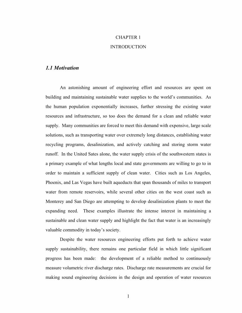
1.1 Motivation

An astonishing amount of engineering effort and resources are spent on

building and maintaining sustainable water supplies to the world’s communities. As

the human population exponentially increases, further stressing the existing water

resources and infrastructure, so too does the demand for a clean and reliable water

supply. Many communities are forced to meet this demand with expensive, large scale

solutions, such as transporting water over extremely long distances, establishing water

recycling programs, desalinization, and actively catching and storing storm water

runoff. In the United Sates alone, the water supply crisis of the southwestern states is

a primary example of what lengths local and state governments are willing to go to in

order to maintain a sufficient supply of clean water. Cities such as Los Angeles,

Phoenix, and Las Vegas have built aqueducts that span thousands of miles to transport

water from remote reservoirs, while several other cities on the west coast such as

Monterey and San Diego are attempting to develop desalinization plants to meet the

expanding need. These examples illustrate the intense interest in maintaining a

sustainable and clean water supply and highlight the fact that water is an increasingly

valuable commodity in today’s society.

Despite the water resources engineering efforts put forth to achieve water

supply sustainability, there remains one particular field in which little significant

progress has been made: the development of a reliable method to continuously

measure volumetric river discharge rates. Discharge rate measurements are crucial for

making sound engineering decisions in the design and operation of water resources

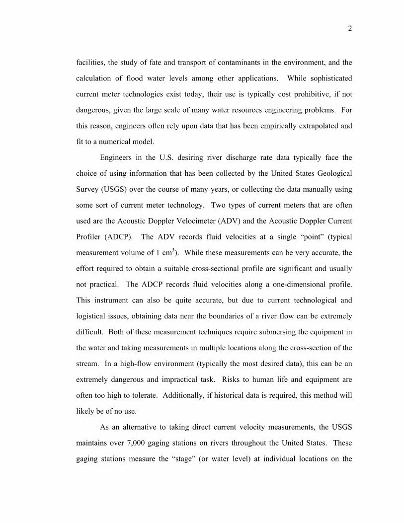
2

facilities, the study of fate and transport of contaminants in the environment, and the

calculation of flood water levels among other applications. While sophisticated

current meter technologies exist today, their use is typically cost prohibitive, if not

dangerous, given the large scale of many water resources engineering problems. For

this reason, engineers often rely upon data that has been empirically extrapolated and

fit to a numerical model.

Engineers in the U.S. desiring river discharge rate data typically face the

choice of using information that has been collected by the United States Geological

Survey (USGS) over the course of many years, or collecting the data manually using

some sort of current meter technology. Two types of current meters that are often

used are the Acoustic Doppler Velocimeter (ADV) and the Acoustic Doppler Current

Profiler (ADCP). The ADV records fluid velocities at a single “point” (typical

measurement volume of 1 cm3). While these measurements can be very accurate, the

effort required to obtain a suitable cross-sectional profile are significant and usually

not practical. The ADCP records fluid velocities along a one-dimensional profile.

This instrument can also be quite accurate, but due to current technological and

logistical issues, obtaining data near the boundaries of a river flow can be extremely

difficult. Both of these measurement techniques require submersing the equipment in

the water and taking measurements in multiple locations along the cross-section of the

stream. In a high-flow environment (typically the most desired data), this can be an

extremely dangerous and impractical task. Risks to human life and equipment are

often too high to tolerate. Additionally, if historical data is required, this method will

likely be of no use.

As an alternative to taking direct current velocity measurements, the USGS

maintains over 7,000 gaging stations on rivers throughout the United States. These

gaging stations measure the “stage” (or water level) at individual locations on the

3

river. In addition to the stage information, engineers deploy to each site on a regular

basis and record direct current velocity measurements using a current meter. With

these two pieces of information, over time a “rating curve” is developed in which

stage is directly related to discharge for that river at that particular location. This data

is typically readily available to the public. Unfortunately, due to sometimes dynamic

bathymetric profiles and rather sparse or non-existent flow data available to allow the

extrapolation of the rating curve to high-volume events, discharge rates calculated

with these curves can be in error ranging from 10 – 70%.

Given the important role that water resource management and engineering will

play in determining the future sustainability of global communities, it has become

imperative to develop a method to continuously, reliably, and accurately measure

volumetric river discharge rates. As other environmental measurement techniques

advance, the limiting factor in calculating the total load of contaminants and sediment

in river outfall is often the overall flow rate. To address this issue, the USGS has

developed the research committee Hydro 21. This group’s stated goal is to “identify

and evaluate new technologies and methods that might have the potential to change

the paradigm in the USGS stream gaging program,” primarily focusing on "non-

contact methods" that could be used in routine river discharge monitoring by direct

measurement of river cross-sectional area, water surface elevation, and water velocity

distribution across the river (http://or.water.usgs.gov/hydro21/index.shtml). Taking

one step toward that goal, this thesis investigates a promising new technique in which

the scalar temperature pattern (STP) on a flowing water surface is thermographically

imaged and tracked and a surface velocity profile is obtained.

This new technique will take advantage of the thermally diverse surface of a

flowing body of turbulent water as it equilibrates with its surroundings. The

momentum flux that takes place at the boundaries of a fluvial flow (primarily at the

4

river bed and the air/water interface) induces turbulence and, therefore, mixing within

the water column. While the turbulent mixing tends to homogenize the thermal

structure of the water column, the inevitable temperature heat flux at the air/water

interface tends to counter this phenomenon. As each parcel of water from the well

mixed water column arrives at the surface the heat exchange takes place rapidly,

ultimately resulting in a thermally diverse air/water interface.

The advantage of having this thermal diversity on the flowing water surface

becomes evident by sequentially thermographically imaging the surface. Given the

proper resolution, spectral sensitivity, and dynamic range, this thermal diversity is

visible to an infrared camera. Viewing these images, one can witness new parcels of

water arriving at the surface, reaching thermal equilibrium with the air, and being

displaced by other new parcels. As this phenomenon occurs, the water surface

continues to move downstream, carrying each of the surface parcels with it. Since the

overall STP maintains its general shape for a substantial amount of time, this

movement can be visually detected and tracked by viewing the sequential images.

The goal of this thesis is to establish a method in which the adaptation of

quantitative imaging (QI) algorithms commonly used in particle image velocimetry

(PIV) can be used to determine a surface velocity profile on a flowing water surface

using infrared thermography. Infrared images of flowing water are captured in a

laboratory setting and several displacement algorithms are tested with Monte Carlo

Simulation and thermographic images, eventually adapting the algorithms to enable

maximum efficiency in determining a comprehensive surface velocity profile.

5

1.2 Literature Review

Significant research has been accomplished in recent years studying and

testing different methods of non-contact river discharge measurement. Many of these

techniques directly apply a hybrid of well-studied QI techniques such as PIV and

particle tracking velocimetry (PTV) in the case of free surface flows. These

velocimetry techniques rely on surface imaging to determine the two-dimensional

flow fields in open channel flows, each with its own unique drawbacks and

advantages. Weitbrecht et al. (2002) used an "off the shelf" PIV package to measure

the two-dimensional surface velocity field and identify the dominant large coherent

structures on a shallow laboratory flow. This method required heavy seeding of the

surface with several different types of buoyant tracers ranging from polystyrene

particles to wooden spheres. While the tracers are generally considered to

satisfactorily trace the actual pathlines of the fluid flow, surface tension in some

conditions can create a problem in which the particles tend to stick together, deviating

from the true pathlines and hence misrepresenting the actual velocity of fluid

movement. Further, these particles integrate over their wetted depth of submergence

and are affected by any air-side motions (i.e., wind). This problem may be mostly

overcome in the laboratory by using surfactants and carefully selecting particle

materials, however the practicality of the overall method in the natural environment is

questionable for a multitude of reasons, including cost effectiveness, environmental

pollution, and reliability.

As an alternative to adding tracer particles to a flow, Creutin et al. (2002)

successfully used natural light reflection off of surface deformations to determine the

two-dimensional flow field. The images recorded were analyzed for brightness

variation and a traditional correlation PIV algorithm was used to determine the desired

6

velocity vector field. Fujita and Tsubaki (2002) presented a variation on this concept

by using a novel synthetic spatio-temporal technique developed to take full advantage

of the assumption that the dominant velocity component is in the streamwise direction.

The result of this non-correlation-based technique is a one-dimensional flow field

across the surface of the channel with a higher spatial resolution in the lateral

direction. While both of these tracerless methods are desirable because they require

no manual seeding of the fluid surface there are some obvious and significant

drawbacks. Since they depend entirely on light reflections off of the surface, these

methods are less accurate when less sunlight is reflected. They will therefore be

useless during night hours, in shaded areas, and even on overcast days.

A seemingly more robust method of non-contact surface velocimetry is

presented by Nicolas et al. (1997). Like the above natural light reflection technique,

this method requires no tracer particles. They used coherent high resolution radar to

image the surface and used a spatio-temporal technique to develop a velocity vector

field. Lee et al. (2002) and Mason et al. (2002) separately present a radar Doppler-

shift based surface velocimetry technique using "binning" to define the two-

dimensional flow field. Both of these seem to provide a solution to the problem of the

inability to take velocity measurements in poor or low light. Yet, they all still suffer

from what almost every other surface velocity measurement technique does: lack of

insight into subsurface velocities. Additionally, these methods are biased by the shear

from wind waves at the surface and have no way of obtaining subsurface velocities.

These are problems that potentially may be solved with the use of sequential

quantitative thermal imaging techniques.

Although velocimetry using thermographic images has scarcely been studied,

some research has been accomplished on the related topics of Scalar Image

Velocimetry (SIV) (Dahm et al., 1992; Su and Dahm, 1996; Pearlstein and Carpenter,

7

1995; Carpenter and Pearlstein, 1996), Correlation Image Velocimetry (CIV)

(Tokumaru and Dimotakis, 1995), and Optical Flow (OF) (Quenot, 1992). The image

analyses range from Direct Numerical Simulation (DNS) images of an arbitrary

passive scalar in 2 and 3 dimensional flows, to laboratory images of known dye-laden

flow regimes (Couette Flow, axis-symmetric turbulent jet, etc…), to satellite imagery

of weather patterns on the surface of Jupiter. The cumulative results of these studies

suggest that, among other methods, a QI-based algorithm may be used to determine

image-flow velocity from images of a passive scalar in a fluid flow.

Hetsroni et al. (2001) successfully used both traditional PIV and Optical Flow

(OF) algorithms to establish a flow field in the lower boundary layer of a fully

developed and artificially heated open channel flow by thermally imaging a piece of

foil on the outside of the lower boundary. The thermal diversity of the flow directly

above the bottom boundary instantly heated the foil, creating a thermal pattern that

could clearly be seen to advect downstream. The assumption that the scalar

temperature field seen on the foil in the infrared could be treated as a proxy tracer for

the fluid velocity was justified. While the techniques developed in this paper are

helpful, they have not been applied on thermographic images of a flowing water

surface.

In addition to temperature being a proxy tracer for fluid motion, researchers

studying mass transfer phenomena at the air/water interface also use it as a tracer for

gas exchange processes. As a result, a number of research efforts have used infrared

thermography on water body surfaces to study and measure mass transfer velocities.

Haussecker, et al (2002) successfully accomplished this measurement (among others)

by sequentially imaging the ocean surface using an infrared camera. The images were

used to verify existing models and theoretical predictions of surface temperature

distributions. Additionally, although fluid flow velocities were not investigated, the

8

images reveal thermal structure on the ocean surface that may enable the use of a QI-

based algorithm to make an accurate velocity measurement.

A similar study by Garbe et al (2003) uses high-resolution infrared

thermography of a laboratory wind driven water surface to further investigate gas

transfer processes. By developing a total derivative method and taking advantage of

the brightness change constraint equation (BCCE – similar to the SIV methods), they

are able to calculate surface renewal rates, verify surface temperature distributions,

and estimate gas transfer velocities. As a byproduct of their effort to determine the

total derivative of these image sequences, a velocity field estimate is obtained.

Although the details are not presented in his paper, Garbe did not use a QI-based

velocimetry technique and a detailed analysis of velocity errors was not presented.

The need for a robust, non-contact volumetric river flow measurement system

has been established. By combining advances in QI displacement algorithms and the

recent accomplishments of gas transfer studies involving thermographic imaging of

flowing water surfaces, this thesis takes the first step in developing a breakthrough

technology that integrates these techniques into a useable and practical surface

velocity profile extraction method. The potential advantages that a quantitative

thermographic image velocimetry system would provide make this initial investigation

into this new technique worth while. Although far beyond the scope of this thesis,

possible benefits of using this system include the fact that the information gathered in

each image may provide crucial information on energy budget analysis and gas

transfer rates, the ability to make uninterrupted river surface velocity measurements,

and the potential insight into subsurface velocities by using feature tracking

technology to measure the velocity of large parcels of hot or cold water traveling

slower or faster than the surrounding surface water and linking them to a certain depth

in the river.

9

CHAPTER 2

EXPERIMENTAL FACILITIES AND METHODS

Quantitatively measuring the surface velocity profile of a uniform fluid flow

using sequential infrared thermography has scarcely been attempted. The use of QI

algorithms as tools to accurately accomplish this measurement introduces a unique set

of challenges which can be overcome by employing the techniques and methods

described in this chapter. Key elements include introducing several methods of

enhancing the signal-to-noise ratio (SNR) of the STPs recorded by an inexpensive

infrared camera in a highly uniform temperature environment.

2.1 Experimental Facility

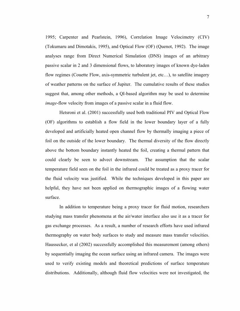
The experiments were carried out in the wide flume constructed in the DeFrees

Hydraulics Laboratory at Cornell University. It is a recirculating type wide open

channel flume allowing generation of spanwise meandering flow motions. As shown

in figure (Figure 1) the flume consists of inlet, test and outlet sections. The test section

is constructed entirely of glass panes allowing excellent optical access (essential for

PIV and Laser Induced Fluorescence (LIF) measurements). It is 15 m in length, 2 m in

width and the maximum water depth is 0.64 m. The flow is driven by two axial pumps

and carried into the inlet section through two 0.406 m diameter PVC pipes beneath the

facility. The rates of the two pumps can be controlled digitally, allowing individual

flow rates to vary either periodically or randomly while maintaining a constant total

flow rate, resulting in enhanced spanwise meandering motion with various length

scales in the test section. In the present study, however, the flow rates of both pumps

10

Q

Workstation

Pumps

Outlet Test section

x

z

Flow

Inlet

Pipe flow

Sandwich type grids

Stainless steel gridWeir

InfraredCamera

ADV

1.07 m

are kept constant at 8 Hz and the depth was kept constant at 30 cm. The flow is

conditioned in the inlet by a series of grids in a sandwich type construction. The grids

are constructed of 5.1 cm deep stainless steel strap with 0.1 m × 0.1 m square

openings. A 2.5 cm thick `horse hair' packing material layer is attached to the top of

the steel grids. These materials are sandwiched between polypropylene molded

thermoplastic mesh sheets. This series of grids is sufficient to break down large

vortices generated by the two pumps and yields a quasi-homogeneous and isotropic

turbulent flow. The turbulence is further conditioned by a nominally 4:1 contraction in

the vertical before entering the test section. A 4 mm polycarbonate rod is mounted

laterally along the junction between the inlet and test section to trip the boundary layer

turbulence. At the end of the test section, a sloping broad crested weir is mounted to

generate super-critical conditions at its crest, preventing free surface perturbations

from reflecting back into the test section (Liao, 2004).

Figure 1: Experimental facility

11

The experimental imaging area was located 10 meters downstream of the

flume entrance. The camera was mounted on the ceiling of the laboratory facility, 2.8

meters above the water surface. This was the maximum separation distance

achievable, therefore limiting the image area due to a fixed camera lens angle of 25o.

Care was taken to align the camera at 90o with respect to the water surface and to align

the image area at 90o with respect to the mean downstream flow direction. The image

area begins at the air/water/flume interface and extends into the center of the flume

1.32 meters, while reaching 1.07 meters in the streamwise direction.

2.2 Infrared Image Collection

Due to the nature of infrared thermography, environmental reflection can

significantly contaminate the true STP of the object being imaged. At the given flow

rate and depth, the surface of the water in the wide flume appears rather unperturbed

to the naked eye. Surface deformations are minor and light is therefore somewhat

clearly reflected. Depending on the angle, wavelength and intensity of external light

sources (among other things), they may appear as extra noise over the image sequence.

Although thermal reflections from the natural environment are unavoidable in a field

setting, Garbe et al. propose a temporal gradient method in which image areas that are

contaminated with environmental reflections are identified and de-weighted during

image processing.

For most of the data sets collected in this thesis, this potential noise source was

avoided by imaging at night with all laboratory lights turned off. Garbe’s reflection

de-weighting technique was therefore not used here, although it may prove to be

valuable in the analysis of future field data.

12

2.2.1 Thermally Equilibrated Flow

In order to test the limits of this proposed velocimetry method, Data Set 1 was

taken under the “worst case” flow conditions. As mentioned previously, due to the

very smooth flume walls and the relatively slow flow velocities, the level of

turbulence in the water is much lower than that typically expected to be found in the

natural environment. Additionally, the water was allowed to approach thermal

equilibrium with the experimental surroundings for several hours prior to collecting

the first data set. With the weaker turbulence carrying fewer and smaller random

parcels of water to the surface and such little temperature difference between the air

and water, these two conditions combine to create a narrow temperature distribution

on the water surface and therefore minimize the STP captured by the infrared camera.

Data Set 2 was collected under the exact same conditions, but the laboratory lights

were turned on.

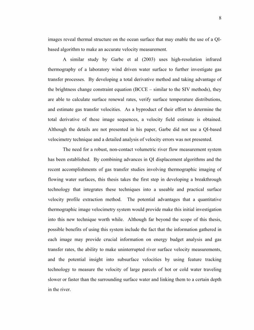
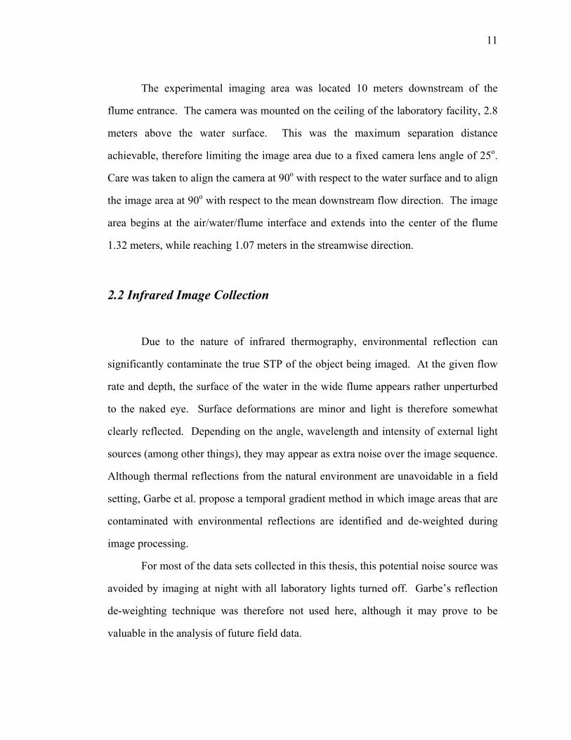
Initial analysis of these “worst case” flow conditions with early versions of the

displacement algorithms raised concerns that the fixed noise level of this specific

camera would obfuscate such a weak signal (Figure 2), making image displacement

analysis a fruitless effort. Images taken on water surfaces of similarly uniform

temperature by superior infrared cameras (such as the one used in the Garbe study)

clearly show a more coherent STP that is expected to provide much better velocimetry

results. Since a camera of this caliber was unavailable for these particular experiments

and ultimately the desire is to work exclusively with low-cost infrared cameras, the

decision was made to physically alter the surface temperature of the flow to obtain an

equally clear STP. This will significantly enhance the SNR similar to the manner in

which traditional PIV technicians seed the flow with particles and artificially

illuminate them.

13

Streamwise Distance [pixels]

Spa

nwis

e D

ista

nce

[pix

els]

20 40 60 80 100 120

20

40

60

80

100

120

140

160

Pix

el In

tens

ity [1

4 bi

t]

-10

-8

-6

-4

-2

0

2

4

6

8

2.2.2 Thermally Disequilibrated Flow

In order to achieve the maximum temperature differential on the flowing water

surface while disrupting the surface flow pattern as little as possible, several thermal

“tagging” methods were tested. This can be accomplished by either cooling or heating

different regions of the flowing water and ensuring that the maximum surface

temperature differential is achieved in the imaging area. Ideally a non-contact method

is desired in which parcels of water are heated or cooled remotely and therefore no

physical obstruction to the water flow is required. This can be achieved using

refrigeration coils at or near the surface or heating coils from beneath the flume.

Using the refrigeration coil method would allow for a uniform or patterned cooling of

the water surface some distance upstream, ultimately allowing the ensuing convective

currents to take place, and drastically diversifying the temperature range on the water

Figure 2: Thermal image (median background removed – see Figure 4 (a) for typical median background image) recorded under “worst case” conditions in which very little thermal diversity exists on the water surface. Flow is from left to right.

14

surface. Similarly a submerged parcel of water that is heated upstream will induce the

reverse convective currents to achieve the same goal. A third alternative exists to

thermally tag the surface anisotropically with a heat source. This buoyant, heated

water will advect downstream, maintaining some form of the imposed structure and

appear as a strong STP in the infrared against the background of the cooler surface

water.

Unfortunately, the resources available for this experiment were limited to

methods that required the introduction of some physical interference with the existing

flow. The first attempt at thermal tagging was to create convective currents by taking

advantage of the temperature difference between ice and the room temperature water

(roughly 25 oC). A mesh bag filled with roughly 100 kg of crushed ice was affixed

along the entire width of the flume upstream of the imaging area. In concept, the

water would flow through the mesh and be cooled as it slowly melted the ice,

eventually sinking as it grew denser. Aside from being exceptionally impractical and

difficult to implement, this method failed simply because the ice melted too quickly

and the mesh bag proved too significant of a disturbance to the surface flow velocities.

Lacking the facilities to build a reliable non-contact method to cool the surface

or heat the subsurface as was accomplished by Mosyak and Hetsroni, 2004, the only

practical alternative was to introduce parcels of buoyant hot water upstream. This was

accomplished with a simple garden hose flowing with hot water. The hose was fitted

with a sprinkler attachment and sprayed evenly on the flowing water surface at several

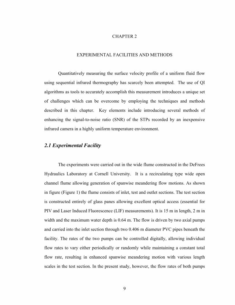
distances upstream. Data Sets 3 and 4 were collected in this manner (Figure 3). This

produced a visible pattern in the thermal images, although the evenness of the

distribution and fineness of the water droplets seemed to diminish the desired effect of

creating a wide thermal diversification. For this reason, the sprinkler head was

removed and the hot water was allowed to flow in bulk through the end of the hose

15

(a) (b) (c)

Streamwise Distance [pixels]

Spa

nwis

e D

ista

nce

[pix

els]

20 40 60 80 100 120

20

40

60

80

100

120

140

160

Pix

el In

tens

ity [1

4 bi

t]

-10

-8

-6

-4

-2

0

2

4

6

8

Streamwise Distance [pixels]

Span

wis

e D

ista

nce

[pix

els]

20 40 60 80 100 120

20

40

60

80

100

120

140

160

Pix

el In

tens

ity [1

4 bi

t]

-10

-8

-6

-4

-2

0

2

4

6

8

Streamwise Distance [pixels]

Spa

nwis

e D

ista

nce

[pix

els]

20 40 60 80 100 120

20

40

60

80

100

120

140

160

Pix

el In

tens

ity [1

4 bi

t]

-10

-8

-6

-4

-2

0

2

4

6

8

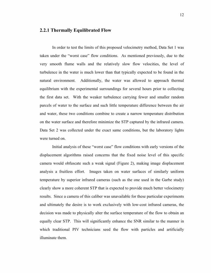
while it was manually moved back and forth across the flume. This method created

more discrete and thermally visible hot parcels of water advecting downstream against

the background of the cool surface water and therefore created the desired STP. Data

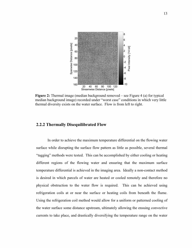
Set 5 was collected in this manner. A comprehensive description of each data set is

presented in Table 1.

Table 1: Data Set Characteristics

Data

Set

Thermal

Tagging

Tagging Distance

Upstream Lights

Sample

Frequency

#

Images

1 None N/A off 30 Hz 10,000

2 None N/A on 30 Hz 10,000

3 Spray 5 m off 30 Hz 10,000

4 Spray 1.5 m off 30 Hz 10,000

5 Bulk 1.5 m off 30 Hz 10,000

Figure 3: Thermal images (median background removed – see Figure 4 (a) for typical median background image) from Data Sets (a) 3, (b) 4, and (c) 5, respectively representing increasing thermal surface diversity. Flow is from left to right.

16

2.3 Velocity Verification

In order to establish a control for this experiment, velocity measurements made

at the water surface by another piece of velocimetry equipment are desired for

comparison. Ideally these measurements can be made in the imaging area laterally

across the surface simultaneously with the collection of the infrared images. For this

experiment, a Nortek Vector ADV was used to obtain point measurements near the

surface. This instrument consisted of a 15 cm probe attached to a 2 m cabled head that

was mounted in an upwards facing position. Due to the limitation of having only one

ADV available, measuring the surface velocity profile simultaneously with collecting

images was not feasible. A single point measurement was made during data collection

directly downstream of the imaging area. This was observed as a rough measurement

of the change in surface water velocity due to the individual seeding methods that

were employed in each set. Immediately following the collection of all five of the

data sets, a surface velocity profile was recorded in the imaging area at an interval of

10 cm under the same exact conditions. Data was sampled at 16 Hz for approximately

60 seconds at each location.

2.4 Camera

The water surface area of interest was imaged using an FLIR Systems

(formerly Indigo Systems) Omega 160 × 128 pixel infrared camera. The camera is

capable of up to 30 frames per second frame transfer, has both 8 bit (256) and 14 bit

(16384) dynamic range modes and a noise-equivalent delta temperature (NEdT) of <

80 mK. A bootstrap uncertainty interval analysis reveals that the typical pixel

intensity 95% confidence interval is +/- 0.12 counts. It is unique in its field as it is

17

drastically less expensive (O($10K) vs. O($100K)) than other infrared cameras of

comparable size and resolution. This is made possible by the distinct difference in

technologies between the expensive and inexpensive infrared cameras. While

traditional, scientific-grade infrared cameras physically count each individual photon

that passes through the filtered lens, ultimately relating the number of photons per

frame to pixel intensity, the inexpensive cameras correlate a bolometric measurement

(i.e. the radiation-induced change in electrical resistance) to pixel intensities.

The software that comes packaged with the camera provides adequate control

over many camera functions such as the automatic flat field correction and video

output modes. Unfortunately, the software is deficient in the areas of file management

and timing control, resulting in an unacceptable limit on total number of captured

images and unpredictable frame drops and repeats. For these reasons Boulder Imaging

of Boulder, Colorado was employed to adapt their Vision Now software to control the

camera and compensate for these problems.

The camera is driven and controlled using an IBM Thinkpad T40 laptop

equipped with a 1.50 GHz Intel Pentium Processor and 512 MB of RAM. Images are

captured by the camera and transferred via IEEE 1394 (FireWire) to an external LaCie

portable hard drive. This system was chosen to maximize performance and portability

to facilitate use in both laboratory and field environments. The Vision Now software

allows for live images to be viewed during data collection. Additionally, live images

may be viewed directly from the FireWire module via an analog output.

The camera lens is fixed with a focal length of 18 mm and a viewing angle of

25°. This narrow angle lens creates the problem of requiring a high overhead clearing

above the water surface that is to be imaged. This issue may be easily overcome in the

future because FLIR Systems now manufactures various other commercial lenses

including a wide angle 8.5 mm lens with a viewing angle of 55º. The image size was

18

calibrated by physically probing the edges of the image area with a heated rod and

measuring the two dimensions of the image area with a measuring tape. It should be

noted that much of the research involved with thermography of flowing water surfaces

has been accomplished using high resolution infrared cameras with very low NEdTs.

This allows the researchers to view extremely fine thermal structure in an environment

that is naturally quite uniform in temperature. A survey of several related papers

regarding gas transfer at the air water interface reveals typical surface water

temperature distributions have a total dynamic range of less than 200 mK. Many of

the infrared cameras used in these research efforts are able to resolve this temperature

difference into a dynamic range of 30 counts (a resolution of less than 10 mK). The

Omega camera used for the research in this paper is only able to resolve a temperature

difference of that magnitude into three to four counts. Since the goal of this

velocimetry technique is to be a widely used and distributed large-scale river

velocimetry device, the need for an extremely expensive camera would likely render

this method impractical. For this reason, one of the long-term focuses of this research

is to determine the minimum camera specifications that will be required to reliably

obtain velocity profile results from a flowing river surface.

19

CHAPTER 3

EXTRACTING SURFACE VELOCITY PROFILES FROM QUANTITATIVE

THERMAL IMAGE SIMULATIONS

This thesis is an investigation into the effectiveness of analyzing sequential

infrared images of a flowing water surface with QI displacement algorithms to extract

the surface velocity profile. In chapter 4 the results of this analysis are presented and

discussed, and in some cases compared to measurements made by the ADV. Before

discussing these results, however, it is essential to understand some of the challenges

that analyzing infrared images with displacement algorithms present. Additionally,

the effectiveness of different types of algorithms and methods are quantified and

compared in this chapter by using Monte Carlo Simulations.

3.1 Background

Traditionally, QI (more specifically, PIV) has been used to obtain a

comprehensive picture of fluid flow velocities in a small scale environment. This

usually involves seeding of the flow in some manner and often requires external

illumination by a light source (e.g. a laser light sheet). The resulting images of

discrete illuminated particles are processed through a correlation algorithm which

determines a mean displacement value for each region of the image and associated

group of particles (and therefore, each parcel of fluid, it is assumed).

While the concept of using a correlation algorithm to compare two sequential

infrared images seems quite similar to traditional PIV, there are several distinct and

important differences. Primarily, as is noted in the SIV research, these images lack the

20

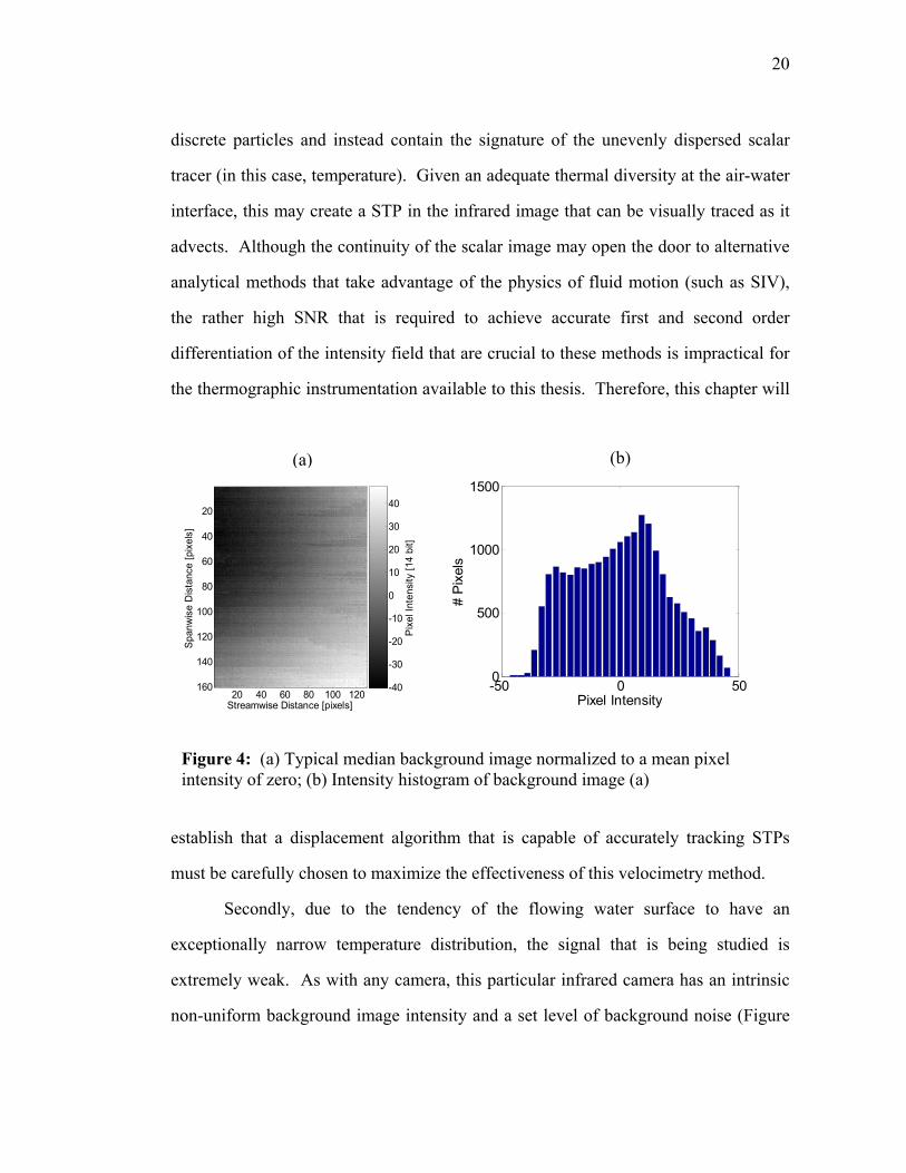
discrete particles and instead contain the signature of the unevenly dispersed scalar

tracer (in this case, temperature). Given an adequate thermal diversity at the air-water

interface, this may create a STP in the infrared image that can be visually traced as it

advects. Although the continuity of the scalar image may open the door to alternative

analytical methods that take advantage of the physics of fluid motion (such as SIV),

the rather high SNR that is required to achieve accurate first and second order

differentiation of the intensity field that are crucial to these methods is impractical for

the thermographic instrumentation available to this thesis. Therefore, this chapter will

establish that a displacement algorithm that is capable of accurately tracking STPs

must be carefully chosen to maximize the effectiveness of this velocimetry method.

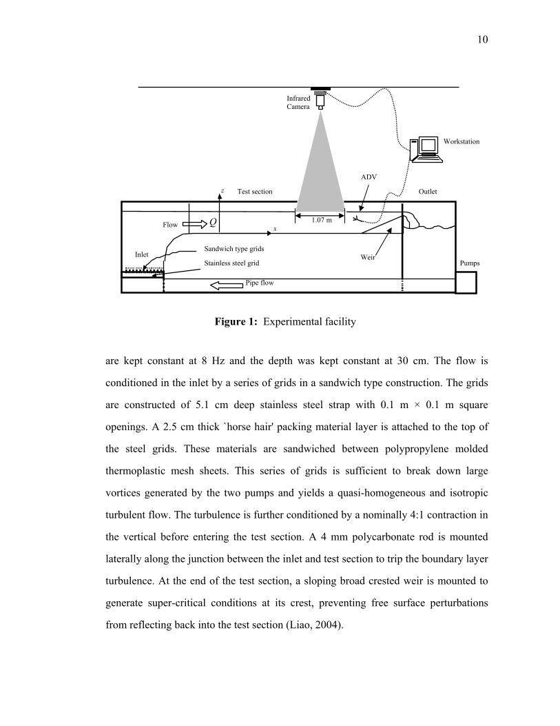
Secondly, due to the tendency of the flowing water surface to have an

exceptionally narrow temperature distribution, the signal that is being studied is

extremely weak. As with any camera, this particular infrared camera has an intrinsic

non-uniform background image intensity and a set level of background noise (Figure

-50 0 500

500

1000

1500

Pixel Intensity

# P

ixel

s(b) (a)

Streamwise Distance [pixels]

Span

wis

e D

ista

nce

[pix

els]

20 40 60 80 100 120

20

40

60

80

100

120

140

160

Pixe

l Int

ensi

ty [1

4 bi

t]

-40

-30

-20

-10

0

10

20

30

40

Figure 4: (a) Typical median background image normalized to a mean pixel intensity of zero; (b) Intensity histogram of background image (a)

21

4). In many of the environments that were imaged, the extremely weak signal was

often obscured by the background image intensity and/or the background noise level.

In other words, the dynamic range of the background can easily be several times larger

than the expected dynamic range of the signal that is being monitored on both the

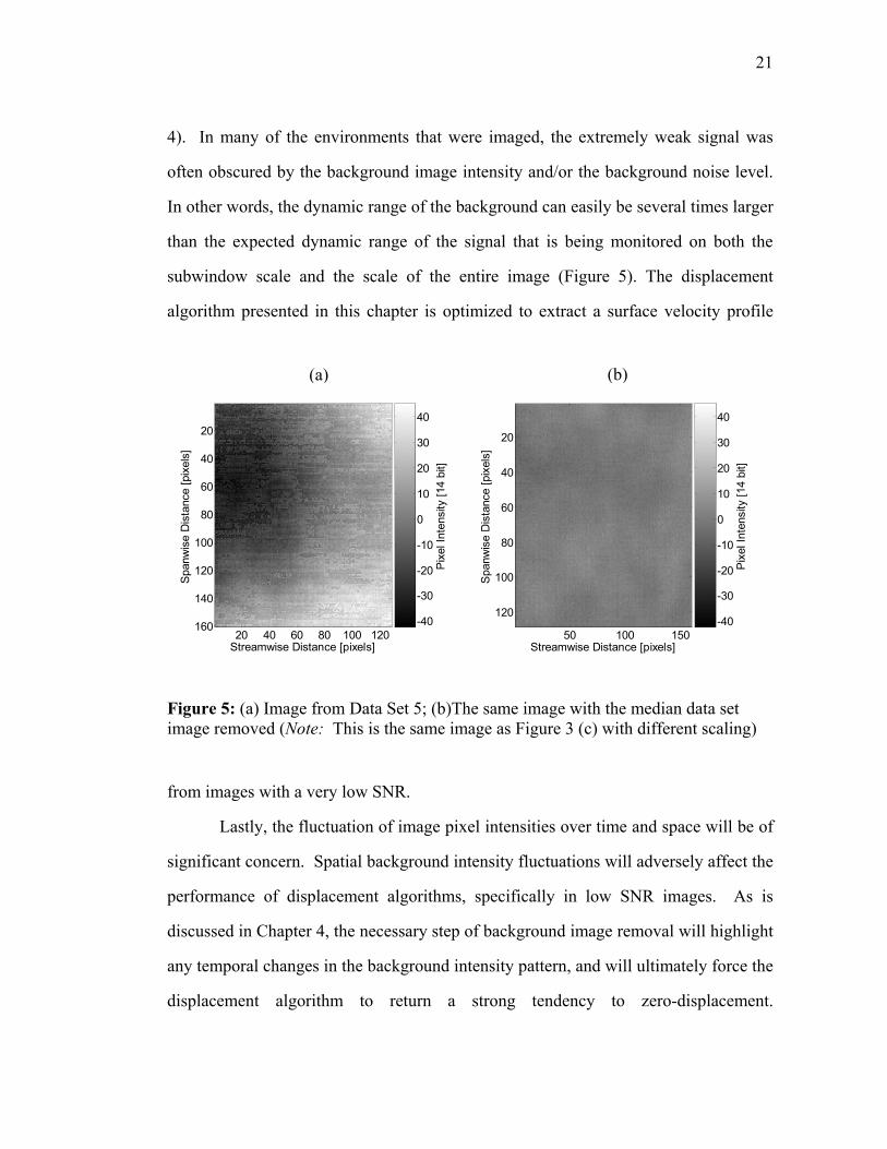
subwindow scale and the scale of the entire image (Figure 5). The displacement

algorithm presented in this chapter is optimized to extract a surface velocity profile

from images with a very low SNR.

Lastly, the fluctuation of image pixel intensities over time and space will be of

significant concern. Spatial background intensity fluctuations will adversely affect the

performance of displacement algorithms, specifically in low SNR images. As is

discussed in Chapter 4, the necessary step of background image removal will highlight

any temporal changes in the background intensity pattern, and will ultimately force the

displacement algorithm to return a strong tendency to zero-displacement.

(a) (b)

Streamwise Distance [pixels]

Spa

nwis

e D

ista

nce

[pix

els]

20 40 60 80 100 120

20

40

60

80

100

120

140

160

Pix

el In

tens

ity [1

4 bi

t]

-40

-30

-20

-10

0

10

20

30

40

Streamwise Distance [pixels]

Spa

nwis

e D

ista

nce

[pix

els]

50 100 150

20

40

60

80

100

120

Pix

el In

tens

ity [1

4 bi

t]

-40

-30

-20

-10

0

10

20

30

40

Figure 5: (a) Image from Data Set 5; (b)The same image with the median data set image removed (Note: This is the same image as Figure 3 (c) with different scaling)

22

Additionally, rapid thermal diffusion of the STP during its short time on the surface of

the water will cause a potentially significant distortion of the pattern that is being

tracked. This pattern distortion reduces the overall effectiveness of the displacement

algorithms. This latter issue can be controlled by the amount of time that is allowed to

pass between surface recordings.

3.2 Monte Carlo Simulation Images

In order to quantitatively test different displacement algorithms and properly

design proposed laboratory and field experiments, a Monte Carlo Simulation image

generator was developed. The goal of this simplistic model was to produce grayscale

images that resemble a thermographic scalar field in flow. For simplicity’s sake, the

generator does not model fluid physics. Similar synthetic images that are based on the

physics of surface renewal, thermal diffusion, and surface temperature distribution

have been developed (Handler et al., 2001); however, that level of detail was not

necessary to carry out the desired comparison of the displacement algorithms in this

thesis. Instead, this generator randomly superimposes several deformed, skewed, and

rotated two-dimensional Gaussian intensity distributions over a blank image. The

distributions of the density and scale of these random shapes were set as variables,

allowing the image to represent the near field or far field. Images were generated on a

trial and error basis while the variables were adjusted until they closely resembled

preliminary thermographic images that were recorded in the laboratory. The images

were then digitally translated using a two sided boundary layer flow modeled with the

1/7th power law. No-slip boundary conditions were established at the flume walls (the

128 pixel edges of the image) and the images were translated a maximum of 10 pixels

per frame pair in the direction perpendicular to these edges.

23

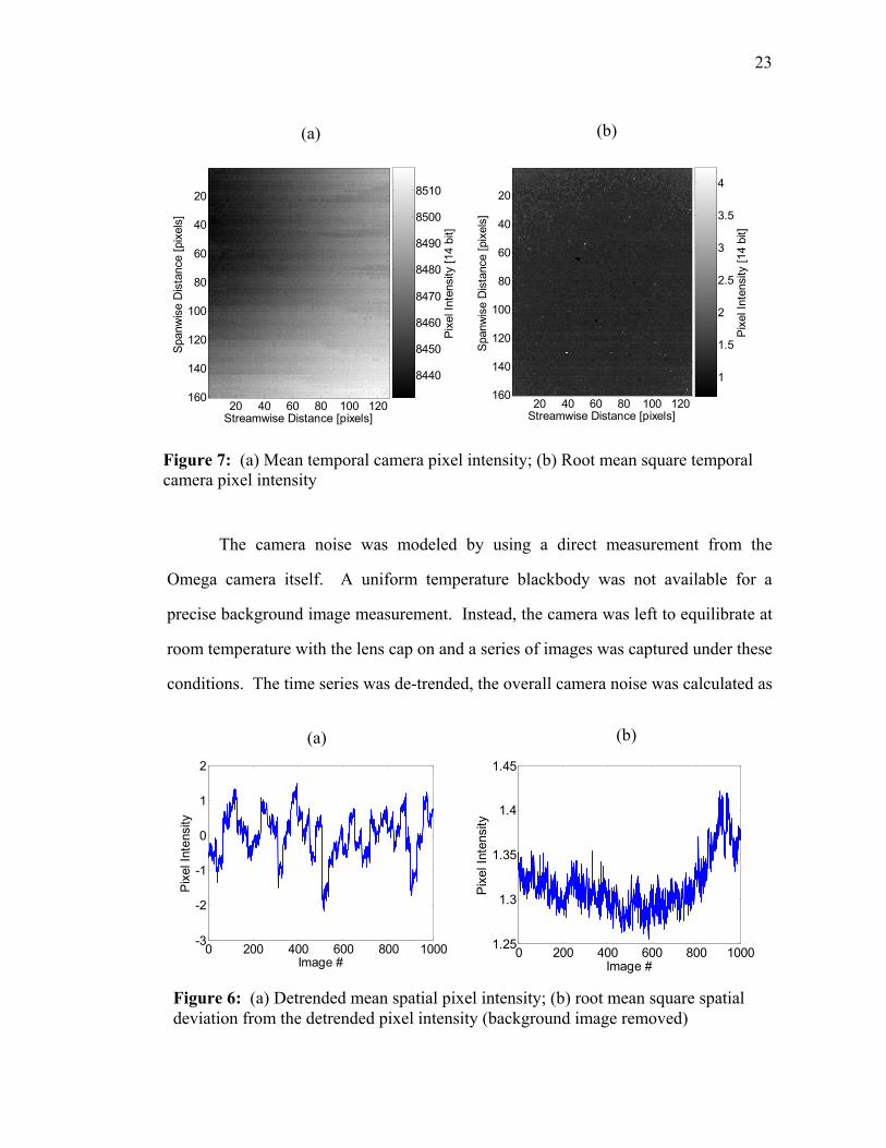
The camera noise was modeled by using a direct measurement from the

Omega camera itself. A uniform temperature blackbody was not available for a

precise background image measurement. Instead, the camera was left to equilibrate at

room temperature with the lens cap on and a series of images was captured under these

conditions. The time series was de-trended, the overall camera noise was calculated as

(a) (b)

Streamwise Distance [pixels]

Span

wis

e D

ista

nce

[pix

els]

20 40 60 80 100 120

20

40

60

80

100

120

140

160

Pixe

l Int

ensi

ty [1

4 bi

t]

8440

8450

8460

8470

8480

8490

8500

8510

Streamwise Distance [pixels]

Spa

nwis

e D

ista

nce

[pix

els]

20 40 60 80 100 120

20

40

60

80

100

120

140

160

Pix

el In

tens

ity [1

4 bi

t]

1

1.5

2

2.5

3

3.5

4

Figure 7: (a) Mean temporal camera pixel intensity; (b) Root mean square temporal camera pixel intensity

(a) (b)

0 200 400 600 800 1000-3

-2

-1

0

1

2

Image #

Pix

el In

tens

ity

0 200 400 600 800 10001.25

1.3

1.35

1.4

1.45

Image #

Pix

el In

tens

ity

Figure 6: (a) Detrended mean spatial pixel intensity; (b) root mean square spatial deviation from the detrended pixel intensity (background image removed)

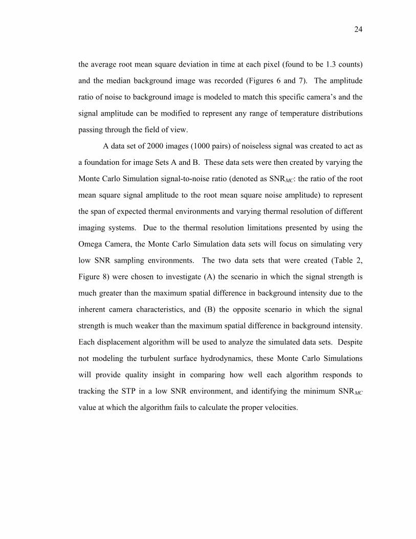
24

the average root mean square deviation in time at each pixel (found to be 1.3 counts)

and the median background image was recorded (Figures 6 and 7). The amplitude

ratio of noise to background image is modeled to match this specific camera’s and the

signal amplitude can be modified to represent any range of temperature distributions

passing through the field of view.

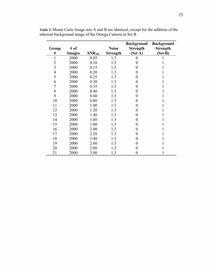
A data set of 2000 images (1000 pairs) of noiseless signal was created to act as

a foundation for image Sets A and B. These data sets were then created by varying the

Monte Carlo Simulation signal-to-noise ratio (denoted as SNRMC: the ratio of the root

mean square signal amplitude to the root mean square noise amplitude) to represent

the span of expected thermal environments and varying thermal resolution of different

imaging systems. Due to the thermal resolution limitations presented by using the

Omega Camera, the Monte Carlo Simulation data sets will focus on simulating very

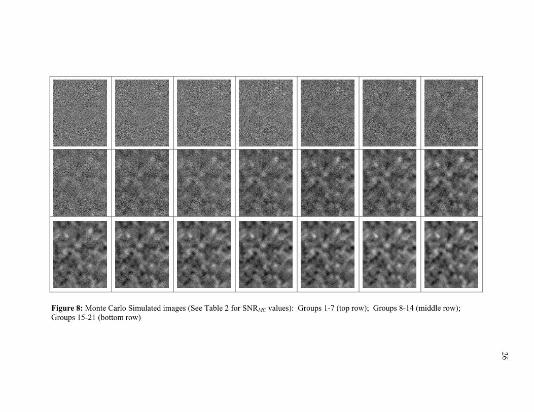
low SNR sampling environments. The two data sets that were created (Table 2,

Figure 8) were chosen to investigate (A) the scenario in which the signal strength is

much greater than the maximum spatial difference in background intensity due to the

inherent camera characteristics, and (B) the opposite scenario in which the signal

strength is much weaker than the maximum spatial difference in background intensity.

Each displacement algorithm will be used to analyze the simulated data sets. Despite

not modeling the turbulent surface hydrodynamics, these Monte Carlo Simulations

will provide quality insight in comparing how well each algorithm responds to

tracking the STP in a low SNR environment, and identifying the minimum SNRMC

value at which the algorithm fails to calculate the proper velocities.

25

Table 2: Monte Carlo Image sets A and B are identical, except for the addition of the inherent background image of the Omega Camera in Set B

Group #

# of Images SNRMC

Noise Strength

Background Strength (Set A)

Background Strength (Set B)

1 2000 0.05 1.3 0 1 2 2000 0.10 1.3 0 1 3 2000 0.15 1.3 0 1 4 2000 0.20 1.3 0 1 5 2000 0.25 1.3 0 1 6 2000 0.30 1.3 0 1 7 2000 0.35 1.3 0 1 8 2000 0.40 1.3 0 1 9 2000 0.60 1.3 0 1 10 2000 0.80 1.3 0 1 11 2000 1.00 1.3 0 1 12 2000 1.20 1.3 0 1 13 2000 1.40 1.3 0 1 14 2000 1.60 1.3 0 1 15 2000 1.80 1.3 0 1 16 2000 2.00 1.3 0 1 17 2000 2.20 1.3 0 1 18 2000 2.40 1.3 0 1 19 2000 2.60 1.3 0 1 20 2000 2.80 1.3 0 1 21 2000 3.00 1.3 0 1

26

Figure 8: Monte Carlo Simulated images (See Table 2 for SNRMC values): Groups 1-7 (top row); Groups 8-14 (middle row); Groups 15-21 (bottom row)

27

3.3 Traditional PIV Analysis

The PIV software developed by Cowen and Monismith (1997) (along with all

of its subsequent upgrades) provided the foundation on which all further QI codes

discussed in this paper were developed. The original version of this algorithm was

intended for use with traditional PIV images. It utilizes a Fast Fourier Transform

(FFT) correlation algorithm and implements several enhancing features such as, image

convolution, subwindow overlap, multiple filters, and data smoothing. The user is

given the flexibility to choose subwindow sizes of 2n × 2n pixels, and therefore has

significant control over the resolution and accuracy. A significant amount of research

has been accomplished on this PIV method, identifying details such as the optimum

particle size, dynamic range and concentration of particles in each subwindow. While

this version is a proven and robust tool in analyzing traditional PIV images, it is yet to

be seen how effective a tool it is for thermographic image analysis.

In order to obtain an understanding of how Cowen’s PIV method will perform

on thermographic images, it is helpful to compare the analysis of traditional synthetic

PIV images with the analysis of the similarly translated Monte Carlo Simulation

images (denoted MC Set 1 for the purposes of this thesis) discussed in the previous

section. To make a fair comparison, both sets of 1000 images have a high SNRMC, are

of equal size (Figure 9) and are subjected to a two-sided boundary layer downstream

translation (Note: This translation pattern is used for all synthetic images in this

thesis). The thermographic simulated images for MC Set 1 are taken from image Set

A, Group 21, as presented in Table 2. The traditional PIV images are created from

Cowen’s image generator (Cowen & Monismith, 1997), with a mean background

noise intensity set to 50 counts (on an 8-bit scale), maximum particle intensity set to

250, particle density of 20 particles per subwindow, and the standard deviation of

28

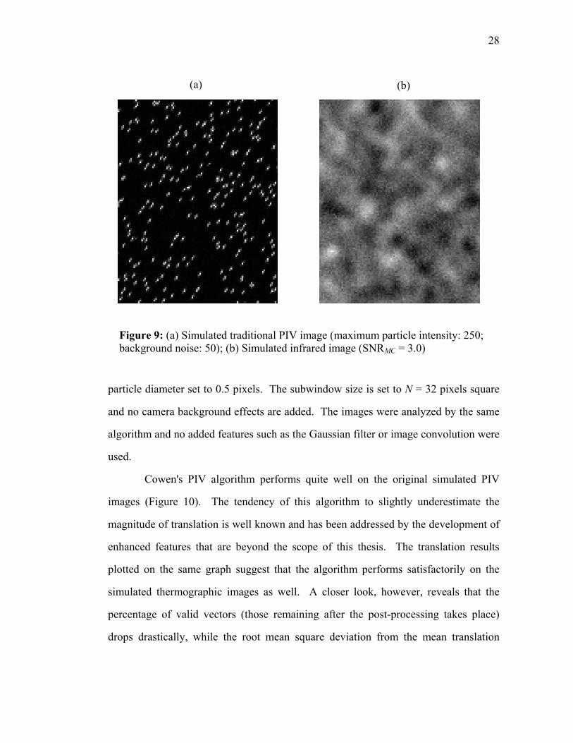
particle diameter set to 0.5 pixels. The subwindow size is set to N = 32 pixels square

and no camera background effects are added. The images were analyzed by the same

algorithm and no added features such as the Gaussian filter or image convolution were

used.

Cowen's PIV algorithm performs quite well on the original simulated PIV

images (Figure 10). The tendency of this algorithm to slightly underestimate the

magnitude of translation is well known and has been addressed by the development of

enhanced features that are beyond the scope of this thesis. The translation results

plotted on the same graph suggest that the algorithm performs satisfactorily on the

simulated thermographic images as well. A closer look, however, reveals that the

percentage of valid vectors (those remaining after the post-processing takes place)

drops drastically, while the root mean square deviation from the mean translation

(a) (b)

Figure 9: (a) Simulated traditional PIV image (maximum particle intensity: 250; background noise: 50); (b) Simulated infrared image (SNRMC = 3.0)

29

vector increases (Table 3). This alone hints at the possibility that this algorithm is not

entirely appropriate for use with these image types.

Furthermore, due to the large size of the subwindow selection relative to the

total image size, the level of resolution leaves much to be desired, resulting in just five

independent data points across the entire image. For this reason, the subwindow size

was reduced to 16 × 16 and the PIV algorithm was again run on MC Set 1. As

expected when reducing the subwindow size, the percentage of valid vectors

decreased and the root mean square deviation increased significantly due to the

reduction in available data to analyze. Unfortunately, the algorithm was unable to

0 50 100 1500

2

4

6

8

10

Image Pixels

Dis

plac

emen

t [P

ixel

s]

Simulated DisplacementPIV Traditional (32 x 32)PIV Simulated IR (32 x 32)PIV Simulated IR (16 x 16)

Figure 10: Cowen’s PIV algorithm results

30

accurately produce a displacement profile that resembled the one actually imposed on

the images (Figure 10).

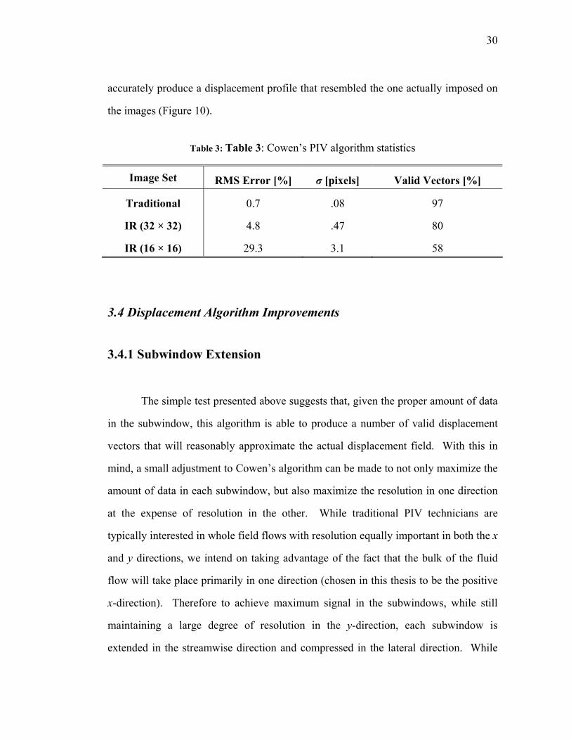
Table 3: Table 3: Cowen’s PIV algorithm statistics

Image Set RMS Error [%] σ [pixels] Valid Vectors [%]

Traditional 0.7 .08 97

IR (32 × 32) 4.8 .47 80

IR (16 × 16) 29.3 3.1 58

3.4 Displacement Algorithm Improvements

3.4.1 Subwindow Extension

The simple test presented above suggests that, given the proper amount of data

in the subwindow, this algorithm is able to produce a number of valid displacement

vectors that will reasonably approximate the actual displacement field. With this in

mind, a small adjustment to Cowen’s algorithm can be made to not only maximize the

amount of data in each subwindow, but also maximize the resolution in one direction

at the expense of resolution in the other. While traditional PIV technicians are

typically interested in whole field flows with resolution equally important in both the x

and y directions, we intend on taking advantage of the fact that the bulk of the fluid

flow will take place primarily in one direction (chosen in this thesis to be the positive

x-direction). Therefore to achieve maximum signal in the subwindows, while still

maintaining a large degree of resolution in the y-direction, each subwindow is

extended in the streamwise direction and compressed in the lateral direction. While

31

the result of this alteration will severely limit the use of this version to unidirectional

flow in the x-direction, the increase in signal is necessary to make it a robust tool in

analyzing these infrared images. For the purposes of this thesis only, this version of

the algorithm will be called “PIV-ext.”

PIV-ext uses the same correlation algorithm as Cowen’s original code, but

simply allows for rectangular subwindows instead of requiring square ones. The

lengths of these subwindows are still constrained (by the nature of the FFT currently

in use) to be of length 2n pixels (Note: This may be easily relaxed at the expense of a

moderate increase in computational time). Test runs quickly indicated that the

maximum resolution while maintaining acceptable accuracy was obtained by using

subwindows of size 8 × 64 pixels. For the Omega camera image resolution, this

allows for a maximum of 19 measured velocities laterally across the image area. .

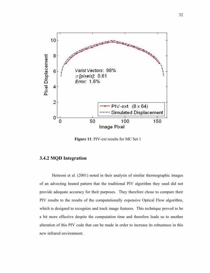
In order to fairly evaluate the effectiveness of this minor alteration, PIV-ext

was used to analyze MC Set 1 also. The results (Figure 11) reveal the success of this

minor alteration as the error is drastically reduced, the resolution is nearly quadrupled,

and the number of valid vectors increases. While these results are very promising

compared with the results of the previous version’s analysis of the same images, they

do not compete quite as well with the analysis of the traditional PIV images.

Additionally, due to the nature of the subwindow size constraints mentioned above,

this algorithm requires that nearly half of the image data be disregarded. To achieve

success in a low SNR environment, clearly as much data as possible must be analyzed,

and therefore further algorithm options are investigated.

32

3.4.2 MQD Integration

Hetsroni et al. (2001) noted in their analysis of similar thermographic images

of an advecting heated pattern that the traditional PIV algorithm they used did not

provide adequate accuracy for their purposes. They therefore chose to compare their

PIV results to the results of the computationally expensive Optical Flow algorithm,

which is designed to recognize and track image features. This technique proved to be

a bit more effective despite the computation time and therefore leads us to another

alteration of this PIV code that can be made in order to increase its robustness in this

new infrared environment.

Figure 11: PIV-ext results for MC Set 1

33

Gui and Merzkitch (2000) presented the Minimum Quadratic Difference

(MQD) algorithm (a least-squared algorithm that, in principle, tracks patterns rather

than individual particles) in an effort to better determine displacement in traditional

PIV images that have non-uniform seeding distribution or non-uniform background

illumination. They successfully demonstrated this technique by comparing their

algorithm to several traditional PIV methods and ultimately showed that the MQD

method was more accurate and much less susceptible to varying particle density and

size distribution. Since our images do not have individual particles, instead having

only a distinct STP advecting downstream, an algorithm that is robust to large changes

in these two variables could potentially perform much better than the traditional

correlation based method.

PIV-ext was adapted to incorporate the MQD method, thereby creating a new

displacement algorithm version which will be referred to as “MQD-ext” for the

remainder of this thesis. Keeping in mind the goals of using the maximum data

available and obtaining fine resolution in the y-direction, the window extension

concept was implemented in this algorithm as well. Due to the small size of these

images and the speed of the computer system involved, computation time was not an

issue and Gui and Merzkirch’s acceleration methods were not employed.

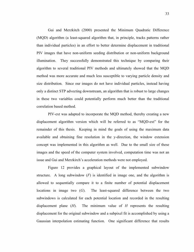
Figure 12 provides a graphical layout of the implemented subwindow

structure. A long subwindow (F) is identified in image one, and the algorithm is

allowed to sequentially compare it to a finite number of potential displacement

locations in image two (G). The least-squared difference between the two

subwindows is calculated for each potential location and recorded in the resulting

displacement plane (H). The minimum value of H represents the resulting

displacement for the original subwindow and a subpixel fit is accomplished by using a

Gaussian interpolation estimating function. One significant difference that results

34

from the use of this algorithm over the original correlation algorithm with an FFT is

that the subwindow data is not assumed to be periodic. While this significantly

diminishes the advantage gained by the central-difference dynamic subwindows

method used in PIV-ext, it also eliminates the ability to evaluate the subpixel fit when

the resulting displacement is found to be on the boundary of H. For this reason,

displacement values are ignored on the boundary of H and these MQD values are

instead used only for subpixel fit interpolation for their inward adjacent MQD values.

Figure 12: MQD-ext subwindow search scheme

To illustrate this, consider the arbitrary MQD peak height H(i,j) in the plane

H(m,n). Although MQD values are calculated for all i < m and j < n, only the values

located at 2 ≤ i ≤ m -1 and 2 ≤ j ≤ n -1 are used to search for MQD peak magnitude. In

the case that the greatest peak magnitude is found to be at H(i,n-1) and the peak

magnitude at H(i,n) happens to be greater than that, the Gaussian sub-pixel fit model

fails, and the displacement vector is rejected. Otherwise, the boundary value is used to

Image 1

Image 2

F G

H G

F

35

appropriately approximate the sub-pixel fit. This issue, of course, can be controlled by

the user in the experimental design (via limiting the time between images within a

pair) and post-analysis design (by defining (m,n) such that all physically realizable

displacements are contained within the usable portion of the plane.

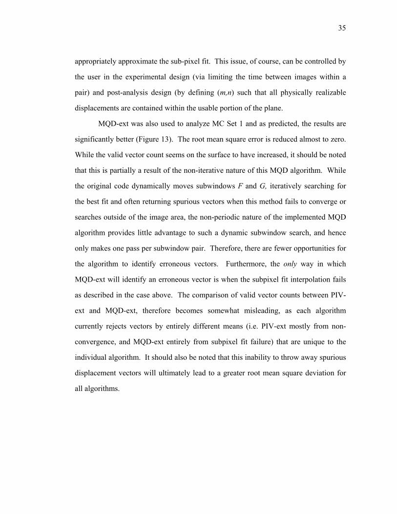
MQD-ext was also used to analyze MC Set 1 and as predicted, the results are

significantly better (Figure 13). The root mean square error is reduced almost to zero.

While the valid vector count seems on the surface to have increased, it should be noted

that this is partially a result of the non-iterative nature of this MQD algorithm. While

the original code dynamically moves subwindows F and G, iteratively searching for

the best fit and often returning spurious vectors when this method fails to converge or

searches outside of the image area, the non-periodic nature of the implemented MQD

algorithm provides little advantage to such a dynamic subwindow search, and hence

only makes one pass per subwindow pair. Therefore, there are fewer opportunities for

the algorithm to identify erroneous vectors. Furthermore, the only way in which

MQD-ext will identify an erroneous vector is when the subpixel fit interpolation fails

as described in the case above. The comparison of valid vector counts between PIV-

ext and MQD-ext, therefore becomes somewhat misleading, as each algorithm

currently rejects vectors by entirely different means (i.e. PIV-ext mostly from non-

convergence, and MQD-ext entirely from subpixel fit failure) that are unique to the

individual algorithm. It should also be noted that this inability to throw away spurious

displacement vectors will ultimately lead to a greater root mean square deviation for

all algorithms.

36

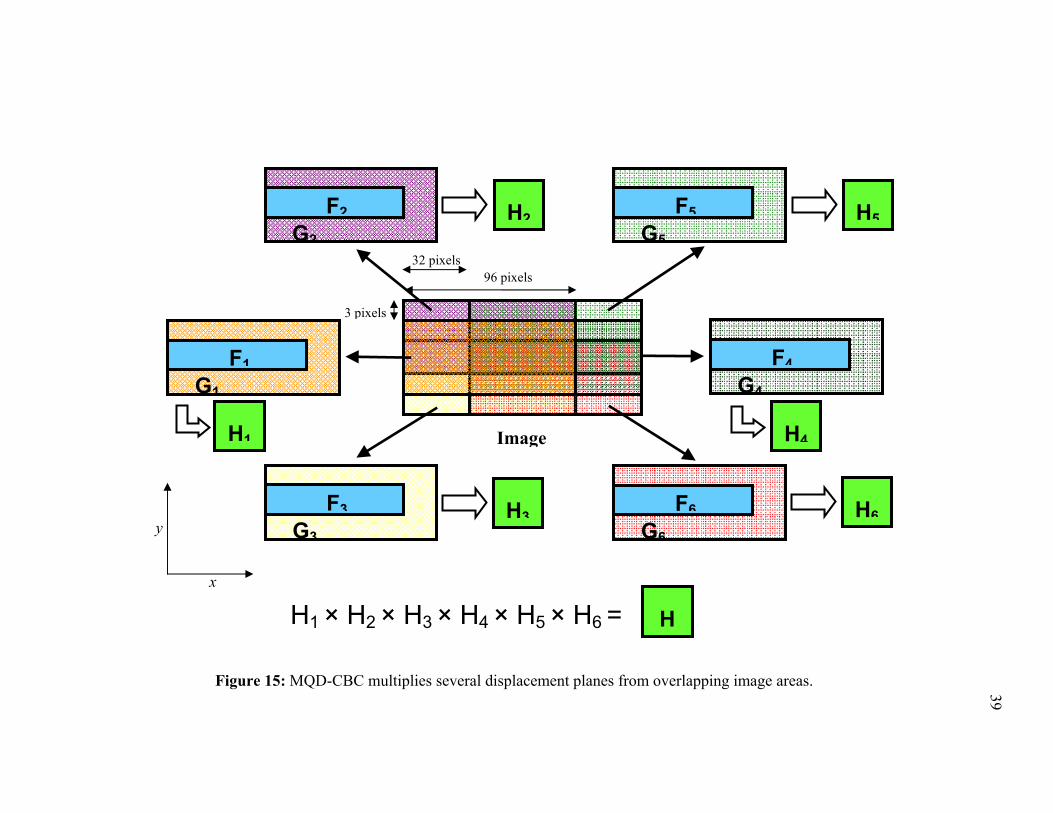
3.4.3 CBC Integration

The results of the MQD-ext analysis on MC Set 1 are quite good and further

algorithm investigation scarcely seems necessary. However, as has been stated earlier,

one of the primary goals of this thesis is to establish that accurate displacement

measurements are possible in an extremely low SNR environment. To further develop

this algorithm to be robust in an environment such as this, one can implement the

correlation based correction (CBC) method presented by Hart (2000). This method

employs a multiplicative noise-canceling technique in which several slightly

overlapping displacement planes from one local area of the image are multiplied on

top of one another. Since the background noise is presumably random while the signal

Figure 13: MQD-ext analysis of MC Set 1

37

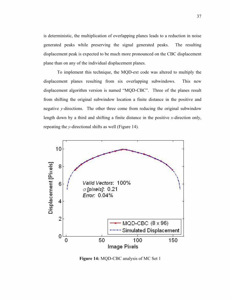
Figure 14: MQD-CBC analysis of MC Set 1

is deterministic, the multiplication of overlapping planes leads to a reduction in noise

generated peaks while preserving the signal generated peaks. The resulting

displacement peak is expected to be much more pronounced on the CBC displacement

plane than on any of the individual displacement planes.

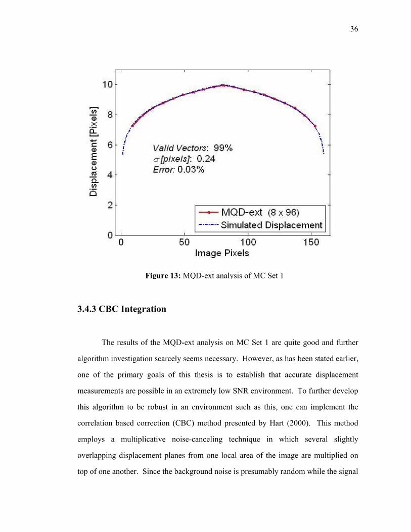
To implement this technique, the MQD-ext code was altered to multiply the

displacement planes resulting from six overlapping subwindows. This new

displacement algorithm version is named “MQD-CBC”. Three of the planes result

from shifting the original subwindow location a finite distance in the positive and

negative y-directions. The other three come from reducing the original subwindow

length down by a third and shifting a finite distance in the positive x-direction only,

repeating the y-directional shifts as well (Figure 14).

38

While these results from MQD-CBC (Figure 15) are nearly indistinguishable

from the results from MQD-ext, further tests on images of much lower SNRs will shed

light on this version’s robustness.

3.4.4 Quantifying the Signal-to-Noise Ratio

It is expected that due to the nearly uniform temperature distributions on the flowing

water surface and the high noise level of the Omega camera, determining

displacements from these thermographic images with the various QI algorithms will

be very difficult. In order to develop another potential comparison between these

algorithms, it is convenient to create a method of quantifying the SNR. For the

further purposes of this thesis, we will define the SNR as the ratio of maximum

magnitude of the displacement plane peak to the median displacement plane value

(Note: This is different from the definition of SNRMC). In order to obtain this value

for MQD-ext and MQD-CBC, the displacement plane is flipped upside down (as

MQD searches for the displacement plane minimum). Furthermore, for MQD-ext and

MQD-CBC, the edge peak magnitudes of the displacement plane will not be

considered in SNR calculations. To make a fair comparison only a limited area (i.e.

comparable displacement values to those resulting from the two MQD algorithms) of

the much larger PIV-ext displacement plane is used for this SNR calculation.

39

32 pixels 96 pixels

y

x

3 pixels

H

G2

F2

G5

F5

G4

F4

G6

F6G3

F3

G1

F1

H2 H5

H3 H6

H1 H4

H1 × H2 × H3 × H4 × H5 × H6 =

Image

Figure 15: MQD-CBC multiplies several displacement planes from overlapping image areas.

40

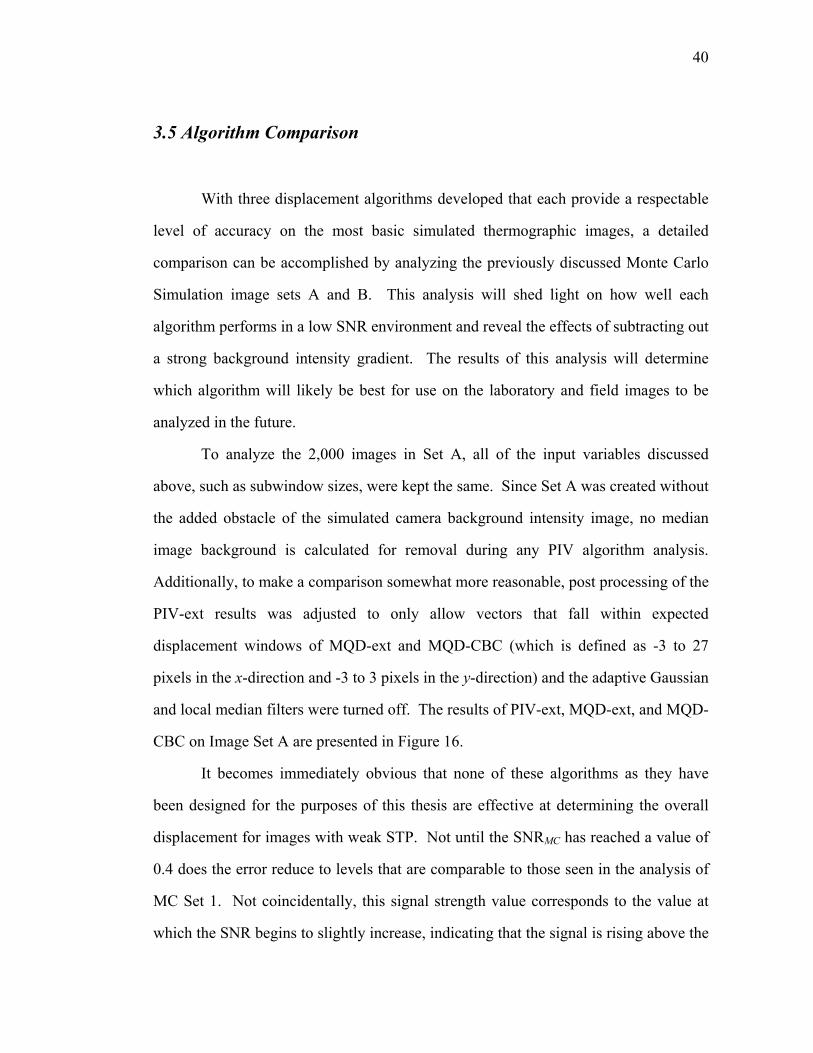
3.5 Algorithm Comparison

With three displacement algorithms developed that each provide a respectable

level of accuracy on the most basic simulated thermographic images, a detailed

comparison can be accomplished by analyzing the previously discussed Monte Carlo

Simulation image sets A and B. This analysis will shed light on how well each

algorithm performs in a low SNR environment and reveal the effects of subtracting out

a strong background intensity gradient. The results of this analysis will determine

which algorithm will likely be best for use on the laboratory and field images to be

analyzed in the future.

To analyze the 2,000 images in Set A, all of the input variables discussed

above, such as subwindow sizes, were kept the same. Since Set A was created without

the added obstacle of the simulated camera background intensity image, no median

image background is calculated for removal during any PIV algorithm analysis.

Additionally, to make a comparison somewhat more reasonable, post processing of the

PIV-ext results was adjusted to only allow vectors that fall within expected

displacement windows of MQD-ext and MQD-CBC (which is defined as -3 to 27

pixels in the x-direction and -3 to 3 pixels in the y-direction) and the adaptive Gaussian

and local median filters were turned off. The results of PIV-ext, MQD-ext, and MQD-

CBC on Image Set A are presented in Figure 16.

It becomes immediately obvious that none of these algorithms as they have

been designed for the purposes of this thesis are effective at determining the overall

displacement for images with weak STP. Not until the SNRMC has reached a value of

0.4 does the error reduce to levels that are comparable to those seen in the analysis of

MC Set 1. Not coincidentally, this signal strength value corresponds to the value at

which the SNR begins to slightly increase, indicating that the signal is rising above the

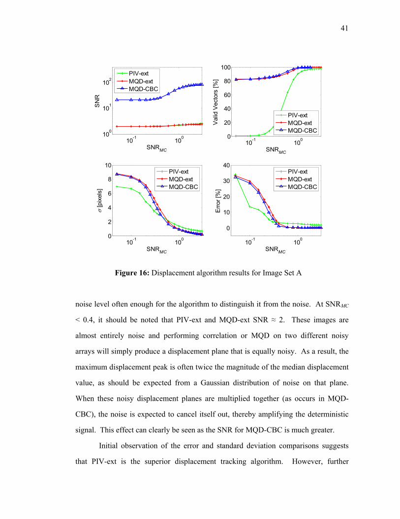
41

noise level often enough for the algorithm to distinguish it from the noise. At SNRMC

< 0.4, it should be noted that PIV-ext and MQD-ext SNR ≈ 2. These images are

almost entirely noise and performing correlation or MQD on two different noisy

arrays will simply produce a displacement plane that is equally noisy. As a result, the

maximum displacement peak is often twice the magnitude of the median displacement

value, as should be expected from a Gaussian distribution of noise on that plane.

When these noisy displacement planes are multiplied together (as occurs in MQD-

CBC), the noise is expected to cancel itself out, thereby amplifying the deterministic

signal. This effect can clearly be seen as the SNR for MQD-CBC is much greater.

Initial observation of the error and standard deviation comparisons suggests

that PIV-ext is the superior displacement tracking algorithm. However, further

10-1 100100

101

102

SN

R

SNRMC10-1 1000

20

40

60

80

100

Val

id V

ecto

rs [%

]

SNRMC

10-1 1000

2

4

6

8

10

SNRMC

σ [p

ixel

s]

10-1 100

0

10

20

30

40

SNRMC

Erro

r [%

]

PIV-extMQD-extMQD-CBC

PIV-extMQD-extMQD-CBC

PIV-extMQD-extMQD-CBC

PIV-extMQD-extMQD-CBC

Figure 16: Displacement algorithm results for Image Set A

42

investigation of the valid vector percentages provides a caveat before reaching this

conclusion. As stated in the previous section, PIV-ext is an iterative correlation

algorithm with an in-built mechanism to discard vectors that are unlikely to have

resulted from a valid correlation. On top of this ability to eliminate spurious vectors,

we artificially discarded vectors that did not fit into the prescribed displacement search

area defined for algorithms MQD-ext and MQD-CBC. The results of these

eliminations can be seen as the percentage of valid vectors is quite low for the regions

in which PIV-ext seems to out-perform the other two algorithms.

Beyond the SNRMC value of 0.4, the algorithms begin to behave as they did in

the initial tests, with MQD-ext performing nearly equally as well as MQD-CBC, and

both of them significantly outperforming PIV-ext. A clearer illustration of why this is

occurring may be obtained by plotting the displacement histograms for valid vectors

obtained from each subwindow in all three algorithms. In image groups that have

SNRMC much greater than 0.4 (Figure 17), MQD-CBC is producing the tightest

distribution of displacement vectors around the proper value (10 pixels), while MQD-

ext has a slightly higher standard deviation, and PIV-ext still higher yet. Note that the

valid vector count for this example is nearly 100% for all three algorithms. On the

-5 0 5 10 15 200

2000

4000

6000

8000Histogram of Xshifts

Displacement [pixels]-5 0 5 10 15 200

2000

4000

6000

8000Histogram of Xshifts

Displacement [pixels]-5 0 5 10 15 200

2000

4000

6000

8000Histogram of Xshifts

Displacement [pixels]

PIV-ext MQD-ext MQD-CBC

Figure 17: Displacement histograms for Group 21, Image Set A

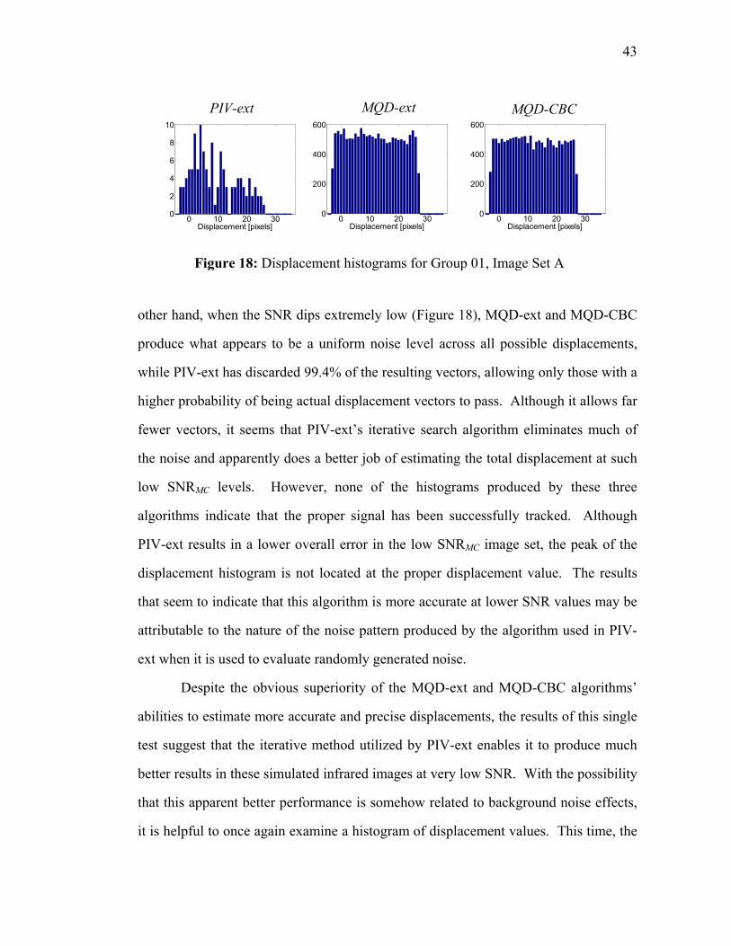
43

other hand, when the SNR dips extremely low (Figure 18), MQD-ext and MQD-CBC

produce what appears to be a uniform noise level across all possible displacements,

while PIV-ext has discarded 99.4% of the resulting vectors, allowing only those with a

higher probability of being actual displacement vectors to pass. Although it allows far

fewer vectors, it seems that PIV-ext’s iterative search algorithm eliminates much of

the noise and apparently does a better job of estimating the total displacement at such

low SNRMC levels. However, none of the histograms produced by these three

algorithms indicate that the proper signal has been successfully tracked. Although

PIV-ext results in a lower overall error in the low SNRMC image set, the peak of the

displacement histogram is not located at the proper displacement value. The results

that seem to indicate that this algorithm is more accurate at lower SNR values may be

attributable to the nature of the noise pattern produced by the algorithm used in PIV-

ext when it is used to evaluate randomly generated noise.

Despite the obvious superiority of the MQD-ext and MQD-CBC algorithms’

abilities to estimate more accurate and precise displacements, the results of this single

test suggest that the iterative method utilized by PIV-ext enables it to produce much

better results in these simulated infrared images at very low SNR. With the possibility

that this apparent better performance is somehow related to background noise effects,

it is helpful to once again examine a histogram of displacement values. This time, the

MQD-CBC

0 10 20 300

200

400

600

Displacement [pixels]

PIV-ext

0 10 20 300

2

4

6

8

10

Displacement [pixels]0 10 20 300

200

400

600

Displacement [pixels]

MQD-ext

Figure 18: Displacement histograms for Group 01, Image Set A

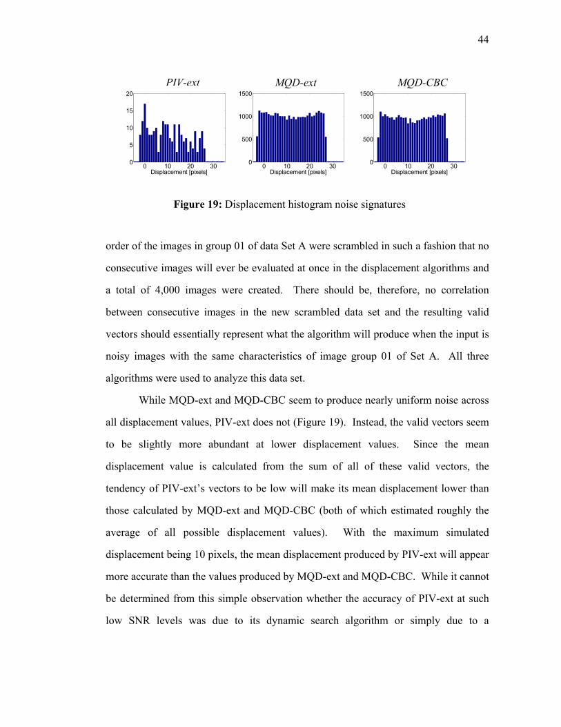
44

order of the images in group 01 of data Set A were scrambled in such a fashion that no

consecutive images will ever be evaluated at once in the displacement algorithms and

a total of 4,000 images were created. There should be, therefore, no correlation

between consecutive images in the new scrambled data set and the resulting valid

vectors should essentially represent what the algorithm will produce when the input is

noisy images with the same characteristics of image group 01 of Set A. All three

algorithms were used to analyze this data set.

While MQD-ext and MQD-CBC seem to produce nearly uniform noise across

all displacement values, PIV-ext does not (Figure 19). Instead, the valid vectors seem

to be slightly more abundant at lower displacement values. Since the mean

displacement value is calculated from the sum of all of these valid vectors, the

tendency of PIV-ext’s vectors to be low will make its mean displacement lower than

those calculated by MQD-ext and MQD-CBC (both of which estimated roughly the

average of all possible displacement values). With the maximum simulated

displacement being 10 pixels, the mean displacement produced by PIV-ext will appear

more accurate than the values produced by MQD-ext and MQD-CBC. While it cannot

be determined from this simple observation whether the accuracy of PIV-ext at such

low SNR levels was due to its dynamic search algorithm or simply due to a

0 10 20 300

500

1000

1500

Displacement [pixels]0 10 20 300

500

1000

1500

Displacement [pixels]

PIV-ext MQD-ext MQD-CBC

0 10 20 300

5

10

15

20

Displacement [pixels]

Figure 19: Displacement histogram noise signatures

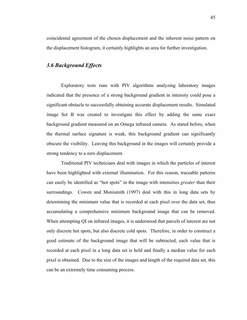
45

coincidental agreement of the chosen displacement and the inherent noise pattern on

the displacement histogram, it certainly highlights an area for further investigation.

3.6 Background Effects

Exploratory tests runs with PIV algorithms analyzing laboratory images

indicated that the presence of a strong background gradient in intensity could pose a

significant obstacle to successfully obtaining accurate displacement results. Simulated

image Set B was created to investigate this effect by adding the same exact

background gradient measured on an Omega infrared camera. As stated before, when

the thermal surface signature is weak, this background gradient can significantly

obscure the visibility. Leaving this background in the images will certainly provide a

strong tendency to a zero displacement.

Traditional PIV technicians deal with images in which the particles of interest

have been highlighted with external illumination. For this reason, traceable patterns

can easily be identified as “hot spots” in the image with intensities greater than their

surroundings. Cowen and Monismith (1997) deal with this in long data sets by

determining the minimum value that is recorded at each pixel over the data set, thus

accumulating a comprehensive minimum background image that can be removed.

When attempting QI on infrared images, it is understood that parcels of interest are not

only discrete hot spots, but also discrete cold spots. Therefore, in order to construct a

good estimate of the background image that will be subtracted, each value that is

recorded at each pixel in a long data set is held and finally a median value for each

pixel is obtained. Due to the size of the images and length of the required data set, this

can be an extremely time consuming process.

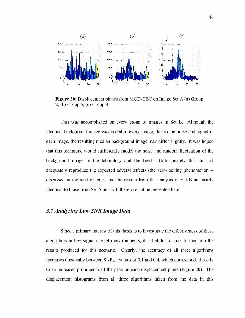
46

This was accomplished on every group of images in Set B. Although the

identical background image was added to every image, due to the noise and signal in

each image, the resulting median background image may differ slightly. It was hoped

that this technique would sufficiently model the noise and random fluctuation of the

background image in the laboratory and the field. Unfortunately this did not

adequately reproduce the expected adverse affects (the zero-locking phenomenon --

discussed in the next chapter) and the results from the analysis of Set B are nearly

identical to those from Set A and will therefore not be presented here.

3.7 Analyzing Low SNR Image Data

Since a primary interest of this thesis is to investigate the effectiveness of these

algorithms in low signal strength environments, it is helpful to look further into the

results produced for this scenario. Clearly, the accuracy of all three algorithms

increases drastically between SNRMC values of 0.1 and 0.4, which corresponds directly

to an increased prominence of the peak on each displacement plane (Figure 20). The

displacement histograms from all three algorithms taken from the data in this

(b) (c) (a)

Figure 20: Displacement planes from MQD-CBC on Image Set A (a) Group 2; (b) Group 5; (c) Group 8

47

transitional signal strength range (Figure 21) highlight the effectiveness of the higher-

order processing feature (iterative dynamic subwindow searching) available to PIV-

ext. The signal is responsible for the peak near the displacement value of 10, while

the analysis of noisy image data is responsible for the uniform noise level that appears

in the MQD-ext and MQD-CBC histograms. Once again, the non-convergent vector

elimination system used in PIV-ext is partially responsible for the shape of that

histogram, and it is unclear how much noise was originally present in the histogram.

The lack of a uniform noise floor, however, suggests that this dynamic subwindow

search algorithm provides superior accuracy for this image group.

3.7 Conclusions

These three displacement algorithms are valuable tools for which to evaluate

simulated thermal images of flowing bodies of water. It is clear that they can be used

to accurately evaluate images with strong signal. As was expected, PIV-ext was

improved upon by the MQD method due to its robustness to noise and pattern

intensity variations. The CBC method, while significantly increasing the SNR, made

only small improvements to the error and precision of the displacement results.

However, the combination of MQD and CBC do, in fact, make for the most accurate

PIV-ext MQD-ext MQD-CBC

0 10 20 300

200

400

600

800

1000

1200

Displacement [pixels]0 10 20 300

500

1000

Displacement [pixels]0 10 20 30

0

50

100

150

200

Displacement [pixels]

Figure 21: Displacement histograms for Image Set B, Group 5

48

algorithm for analysis of these Monte Carlo Simulation images of sufficiently high

SNRMC values.

The other important finding garnered from the comparison of these three

algorithms is that although PIV-ext’s dynamic subwindow vector elimination method

discards nearly 100% of the vectors at extremely low SNRMC (Figure 18), it is not at

all clear that the passing vectors are actually valid. Only in the transitional SNRMC

range (Figure 21) do we begin to see that this spurious vector elimination system may

provide PIV-ext an advantage over the other two MQD based algorithms. Therefore,

although we know that, on the whole, the MQD algorithms outperform the PIV

algorithm, a reliable method in which to eliminate the noise floor that is currently

associated with these displacement histograms must be implemented.

At first glance, it may be obvious to the reader that using an adaptive Gaussian

filter would solve this problem easily. While this would be ineffective on the

extremely low SNRMC image sets, it would be quite effective if used on the results

from all three algorithms in the transitional range. Additionally, the implementation

of a local median filter (elimination based on the magnitude of a vector’s neighbors) is

not entirely practical, due to the lack of surrounding vectors. Unfortunately, as will be

presented in the next section, the use of the adaptive Gaussian filter becomes

ineffective when used in the analysis of real thermal images of a flowing body of

water.

49

CHAPTER 4

EXTRACTING SURFACE VELOCITY PROFILES FROM QUANTITATIVE

THERMAL LABORATORY IMAGES

Although the previous chapter depicts that accurate results can be obtained by

applying the displacement algorithms to simulated infrared images, proof must also be

established that they can adequately extract surface velocity from thermographic

laboratory images. The five data sets that were collected in the large flume described

in chapter 2 were specifically designed to establish proof that these algorithms can be

used to extract surface velocity and ultimately to test the limits of this capability in

highly uniform temperature environments. In this chapter the laboratory

thermographic images are analyzed with the previously developed displacement

algorithms.

4.1 Thermally Disequilibrated Flows

As described in chapter 2, the flow recorded in Data Set 5 was heavily

disequilibrated by adding warm water in bulk from the nozzle of a hose. Since the

SNR for this image set is sufficiently high, all three of the displacement algorithms

perform quite well in extracting the correct surface velocity. For simplicity’s sake,

only the results from MQD-CBC analysis are presented, as it provided the most

precise (i.e. lowest standard deviation) displacement values at high SNR. A detailed

quantitative analysis of rms error will not be presented in this thesis. The ADV

velocity data was not collected simultaneously with each image set and since the

physical act of disrupting the flow with bulk flow from a hose nozzle likely biased the

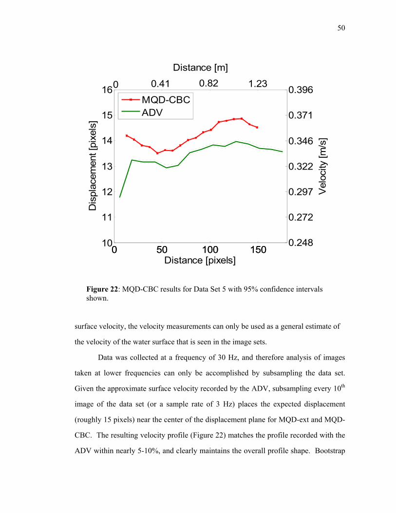
50

surface velocity, the velocity measurements can only be used as a general estimate of

the velocity of the water surface that is seen in the image sets.

Data was collected at a frequency of 30 Hz, and therefore analysis of images

taken at lower frequencies can only be accomplished by subsampling the data set.

Given the approximate surface velocity recorded by the ADV, subsampling every 10th

image of the data set (or a sample rate of 3 Hz) places the expected displacement

(roughly 15 pixels) near the center of the displacement plane for MQD-ext and MQD-

CBC. The resulting velocity profile (Figure 22) matches the profile recorded with the

ADV within nearly 5-10%, and clearly maintains the overall profile shape. Bootstrap

0 50 100 15010

11

12

13

14

15

16D

ispl

acem

ent [

pixe

ls]

0 50 100 1500.248

0.272

0.297

0.322

0.346

0.371

0.396

Distance [pixels]

Vel

ocity

[m/s

]

Distance [m]

MQD-CBCADV

0.41 0.82 1.230

Figure 22: MQD-CBC results for Data Set 5 with 95% confidence intervals shown.

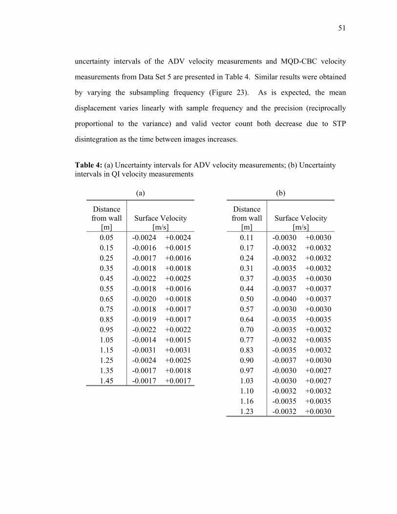
51

uncertainty intervals of the ADV velocity measurements and MQD-CBC velocity

measurements from Data Set 5 are presented in Table 4. Similar results were obtained

by varying the subsampling frequency (Figure 23). As is expected, the mean

displacement varies linearly with sample frequency and the precision (reciprocally

proportional to the variance) and valid vector count both decrease due to STP

disintegration as the time between images increases.

Table 4: (a) Uncertainty intervals for ADV velocity measurements; (b) Uncertainty intervals in QI velocity measurements

(a) (b)

Distance from wall

[m] Surface Velocity

[m/s] 0.05 -0.0024 +0.00240.15 -0.0016 +0.00150.25 -0.0017 +0.00160.35 -0.0018 +0.00180.45 -0.0022 +0.00250.55 -0.0018 +0.00160.65 -0.0020 +0.00180.75 -0.0018 +0.00170.85 -0.0019 +0.00170.95 -0.0022 +0.00221.05 -0.0014 +0.00151.15 -0.0031 +0.00311.25 -0.0024 +0.00251.35 -0.0017 +0.00181.45 -0.0017 +0.0017

Distance from wall

[m] Surface Velocity

[m/s] 0.11 -0.0030 +0.00300.17 -0.0032 +0.00320.24 -0.0032 +0.00320.31 -0.0035 +0.00320.37 -0.0035 +0.00300.44 -0.0037 +0.00370.50 -0.0040 +0.00370.57 -0.0030 +0.00300.64 -0.0035 +0.00350.70 -0.0035 +0.00320.77 -0.0032 +0.00350.83 -0.0035 +0.00320.90 -0.0037 +0.00300.97 -0.0030 +0.00271.03 -0.0030 +0.00271.10 -0.0032 +0.00321.16 -0.0035 +0.00351.23 -0.0032 +0.0030

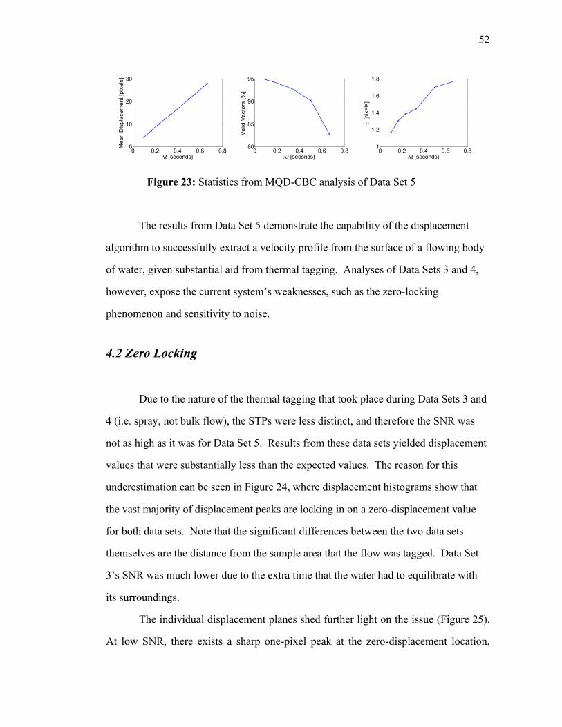
52

The results from Data Set 5 demonstrate the capability of the displacement

algorithm to successfully extract a velocity profile from the surface of a flowing body

of water, given substantial aid from thermal tagging. Analyses of Data Sets 3 and 4,

however, expose the current system’s weaknesses, such as the zero-locking

phenomenon and sensitivity to noise.

4.2 Zero Locking

Due to the nature of the thermal tagging that took place during Data Sets 3 and

4 (i.e. spray, not bulk flow), the STPs were less distinct, and therefore the SNR was

not as high as it was for Data Set 5. Results from these data sets yielded displacement

values that were substantially less than the expected values. The reason for this

underestimation can be seen in Figure 24, where displacement histograms show that

the vast majority of displacement peaks are locking in on a zero-displacement value

for both data sets. Note that the significant differences between the two data sets

themselves are the distance from the sample area that the flow was tagged. Data Set

3’s SNR was much lower due to the extra time that the water had to equilibrate with

its surroundings.

The individual displacement planes shed further light on the issue (Figure 25).

At low SNR, there exists a sharp one-pixel peak at the zero-displacement location,

0 0.2 0.4 0.6 0.80

10

20

30

∆t [seconds]

Mea

n D

ispl

acem

ent [

pixe

ls]

0 0.2 0.4 0.6 0.880

85

90

95

∆t [seconds]

Val

id V

ecto

rs [%

]

0 0.2 0.4 0.6 0.81

1.2

1.4

1.6

1.8

∆t [seconds]

σ [p

ixel

s]

Figure 23: Statistics from MQD-CBC analysis of Data Set 5

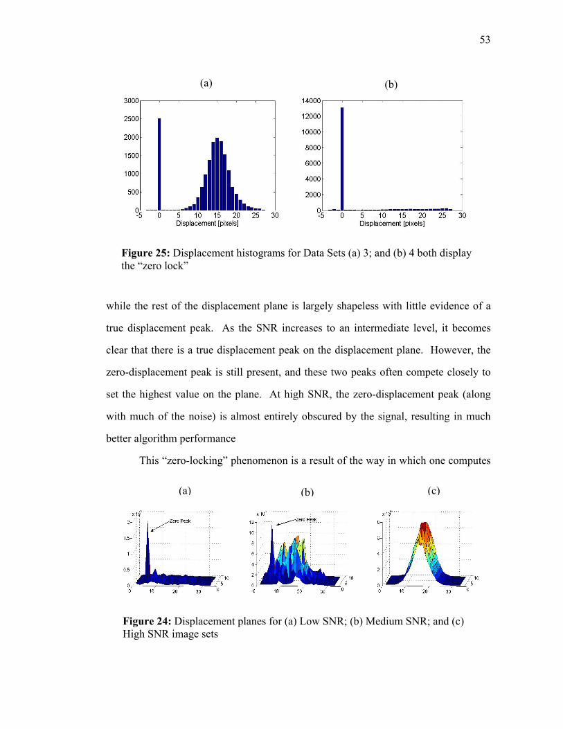
53

while the rest of the displacement plane is largely shapeless with little evidence of a

true displacement peak. As the SNR increases to an intermediate level, it becomes

clear that there is a true displacement peak on the displacement plane. However, the

zero-displacement peak is still present, and these two peaks often compete closely to

set the highest value on the plane. At high SNR, the zero-displacement peak (along

with much of the noise) is almost entirely obscured by the signal, resulting in much

better algorithm performance

This “zero-locking” phenomenon is a result of the way in which one computes

(a) (b)

Figure 25: Displacement histograms for Data Sets (a) 3; and (b) 4 both display the “zero lock”

(a) (b) (c)

Figure 24: Displacement planes for (a) Low SNR; (b) Medium SNR; and (c) High SNR image sets

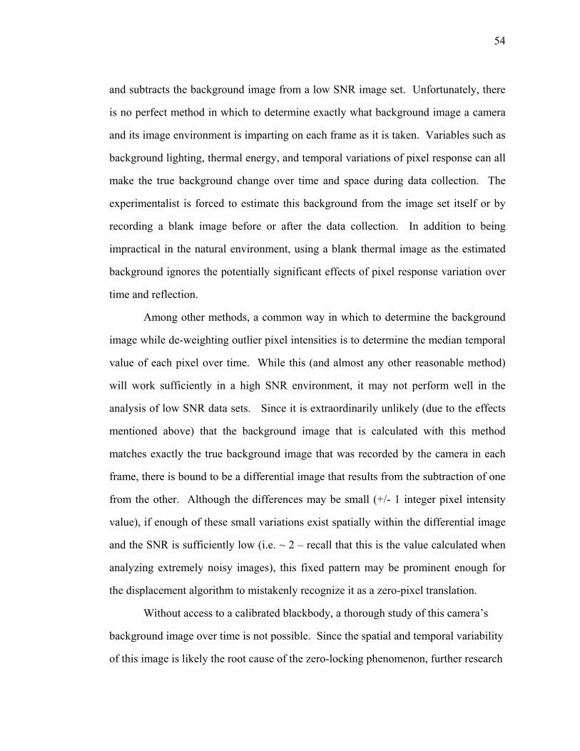
54

and subtracts the background image from a low SNR image set. Unfortunately, there

is no perfect method in which to determine exactly what background image a camera

and its image environment is imparting on each frame as it is taken. Variables such as

background lighting, thermal energy, and temporal variations of pixel response can all

make the true background change over time and space during data collection. The

experimentalist is forced to estimate this background from the image set itself or by

recording a blank image before or after the data collection. In addition to being

impractical in the natural environment, using a blank thermal image as the estimated

background ignores the potentially significant effects of pixel response variation over

time and reflection.

Among other methods, a common way in which to determine the background

image while de-weighting outlier pixel intensities is to determine the median temporal

value of each pixel over time. While this (and almost any other reasonable method)

will work sufficiently in a high SNR environment, it may not perform well in the

analysis of low SNR data sets. Since it is extraordinarily unlikely (due to the effects

mentioned above) that the background image that is calculated with this method

matches exactly the true background image that was recorded by the camera in each

frame, there is bound to be a differential image that results from the subtraction of one

from the other. Although the differences may be small (+/- 1 integer pixel intensity

value), if enough of these small variations exist spatially within the differential image

and the SNR is sufficiently low (i.e. ~ 2 – recall that this is the value calculated when

analyzing extremely noisy images), this fixed pattern may be prominent enough for

the displacement algorithm to mistakenly recognize it as a zero-pixel translation.

Without access to a calibrated blackbody, a thorough study of this camera’s

background image over time is not possible. Since the spatial and temporal variability

of this image is likely the root cause of the zero-locking phenomenon, further research

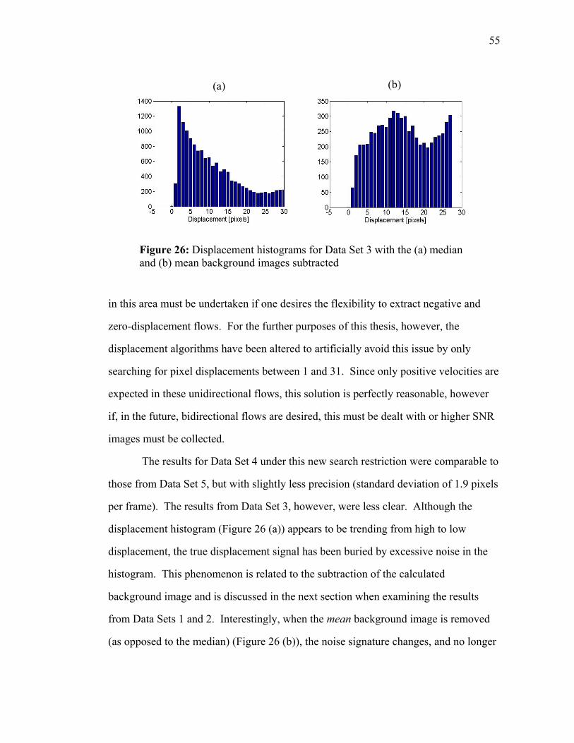
55

in this area must be undertaken if one desires the flexibility to extract negative and

zero-displacement flows. For the further purposes of this thesis, however, the

displacement algorithms have been altered to artificially avoid this issue by only

searching for pixel displacements between 1 and 31. Since only positive velocities are

expected in these unidirectional flows, this solution is perfectly reasonable, however

if, in the future, bidirectional flows are desired, this must be dealt with or higher SNR

images must be collected.

The results for Data Set 4 under this new search restriction were comparable to

those from Data Set 5, but with slightly less precision (standard deviation of 1.9 pixels

per frame). The results from Data Set 3, however, were less clear. Although the

displacement histogram (Figure 26 (a)) appears to be trending from high to low

displacement, the true displacement signal has been buried by excessive noise in the

histogram. This phenomenon is related to the subtraction of the calculated

background image and is discussed in the next section when examining the results

from Data Sets 1 and 2. Interestingly, when the mean background image is removed

(as opposed to the median) (Figure 26 (b)), the noise signature changes, and no longer

(a) (b)

Figure 26: Displacement histograms for Data Set 3 with the (a) median and (b) mean background images subtracted

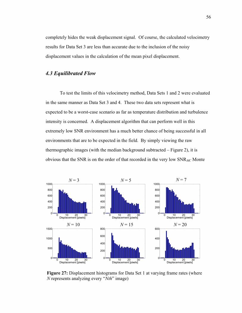
56

completely hides the weak displacement signal. Of course, the calculated velocimetry

results for Data Set 3 are less than accurate due to the inclusion of the noisy

displacement values in the calculation of the mean pixel displacement.

4.3 Equilibrated Flow

To test the limits of this velocimetry method, Data Sets 1 and 2 were evaluated

in the same manner as Data Set 3 and 4. These two data sets represent what is

expected to be a worst-case scenario as far as temperature distribution and turbulence

intensity is concerned. A displacement algorithm that can perform well in this

extremely low SNR environment has a much better chance of being successful in all

environments that are to be expected in the field. By simply viewing the raw

thermographic images (with the median background subtracted – Figure 2), it is

obvious that the SNR is on the order of that recorded in the very low SNRMC Monte

0 10 20 300

200

400

600

800

1000

Displacement [pixels]

N = 3

0 10 20 300

200

400

600

800

1000

Displacement [pixels]0 10 20 300

200

400

600

800

1000

Displacement [pixels]

0 10 20 300

500

1000

1500

Displacement [pixels]0 10 20 300

200

400

600

800

Displacement [pixels]0 10 20 300

200

400

600

Displacement [pixels]

N = 5 N = 7

N = 10 N = 15 N = 20

Figure 27: Displacement histograms for Data Set 1 at varying frame rates (where N represents analyzing every “Nth” image)

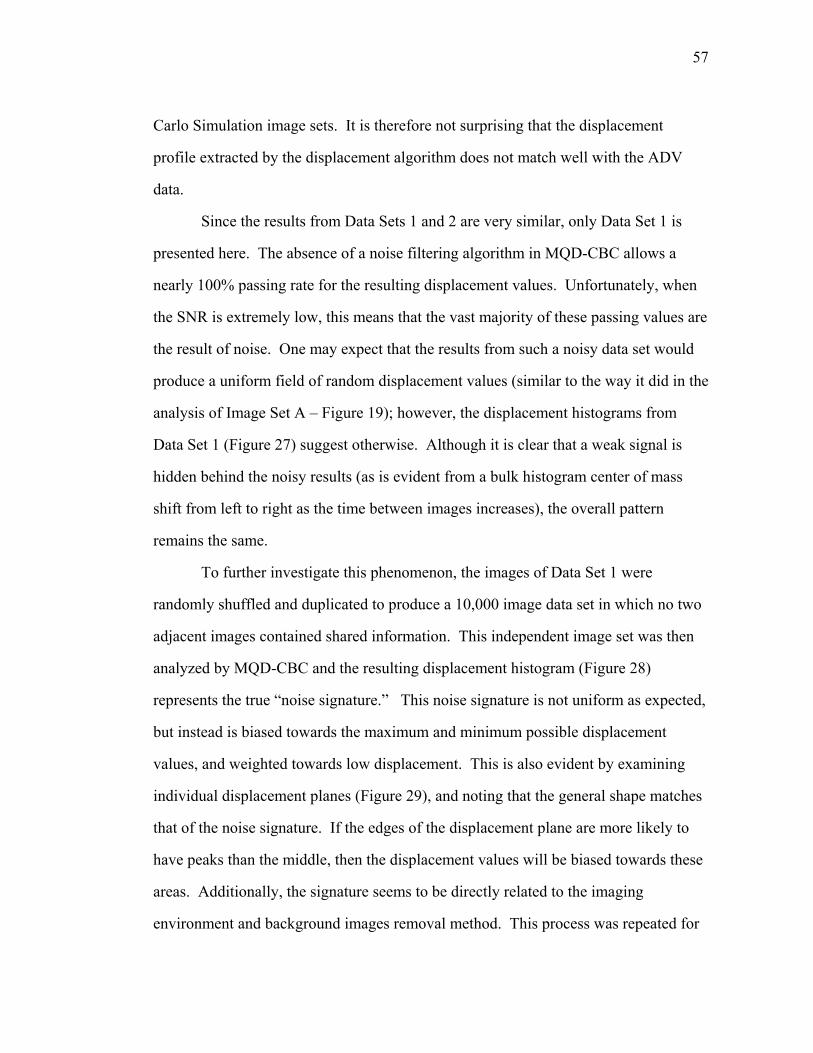
57

Carlo Simulation image sets. It is therefore not surprising that the displacement

profile extracted by the displacement algorithm does not match well with the ADV

data.

Since the results from Data Sets 1 and 2 are very similar, only Data Set 1 is

presented here. The absence of a noise filtering algorithm in MQD-CBC allows a

nearly 100% passing rate for the resulting displacement values. Unfortunately, when

the SNR is extremely low, this means that the vast majority of these passing values are

the result of noise. One may expect that the results from such a noisy data set would

produce a uniform field of random displacement values (similar to the way it did in the

analysis of Image Set A – Figure 19); however, the displacement histograms from

Data Set 1 (Figure 27) suggest otherwise. Although it is clear that a weak signal is

hidden behind the noisy results (as is evident from a bulk histogram center of mass

shift from left to right as the time between images increases), the overall pattern

remains the same.

To further investigate this phenomenon, the images of Data Set 1 were

randomly shuffled and duplicated to produce a 10,000 image data set in which no two

adjacent images contained shared information. This independent image set was then

analyzed by MQD-CBC and the resulting displacement histogram (Figure 28)

represents the true “noise signature.” This noise signature is not uniform as expected,

but instead is biased towards the maximum and minimum possible displacement

values, and weighted towards low displacement. This is also evident by examining

individual displacement planes (Figure 29), and noting that the general shape matches

that of the noise signature. If the edges of the displacement plane are more likely to

have peaks than the middle, then the displacement values will be biased towards these

areas. Additionally, the signature seems to be directly related to the imaging

environment and background images removal method. This process was repeated for

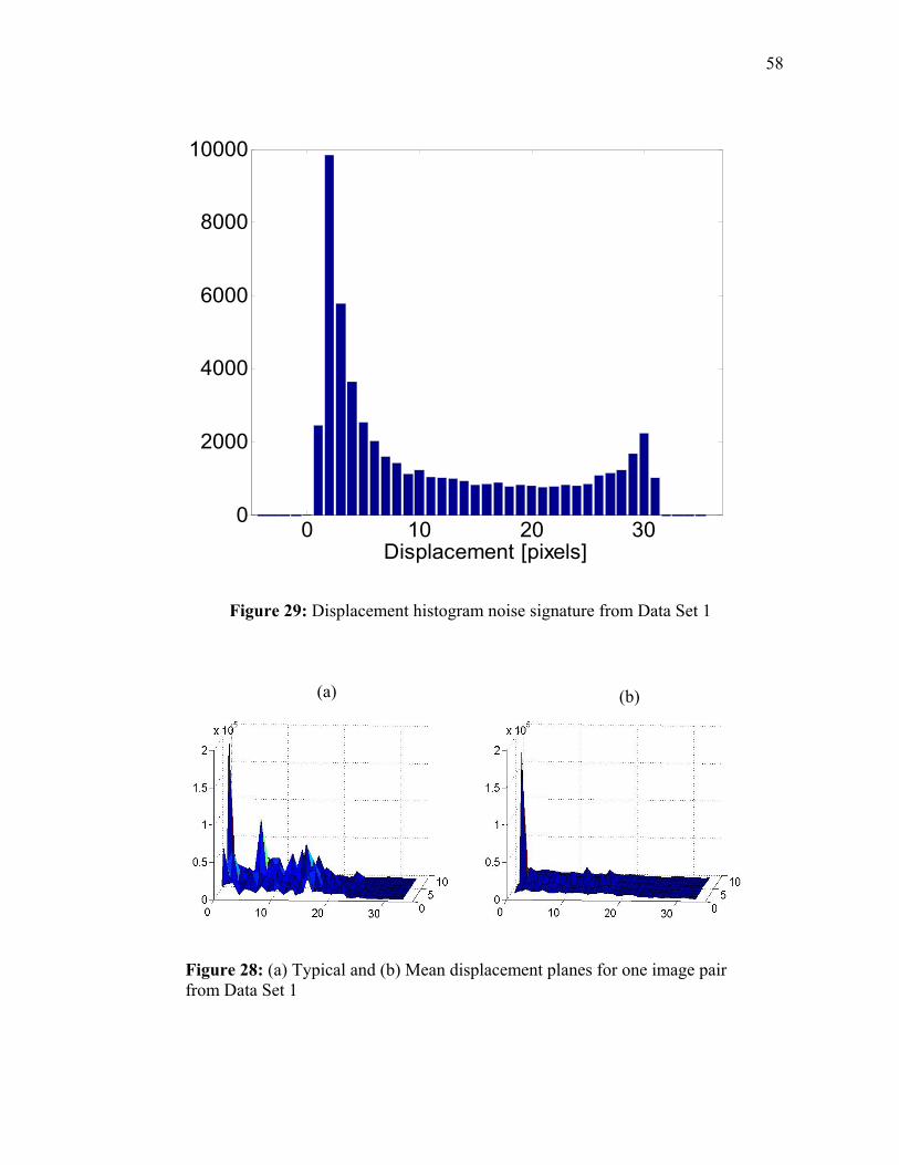
58

0 10 20 300

2000

4000

6000

8000

10000

Displacement [pixels]

Figure 29: Displacement histogram noise signature from Data Set 1

(a) (b)

Figure 28: (a) Typical and (b) Mean displacement planes for one image pair from Data Set 1

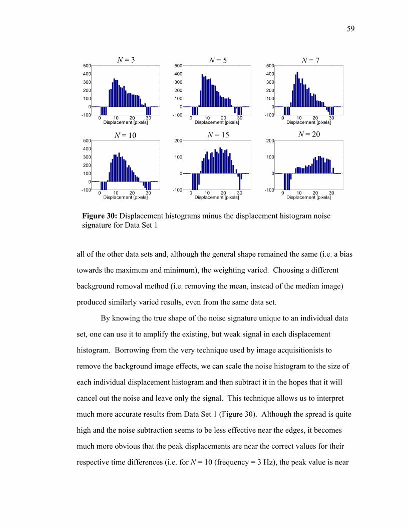
59

all of the other data sets and, although the general shape remained the same (i.e. a bias

towards the maximum and minimum), the weighting varied. Choosing a different

background removal method (i.e. removing the mean, instead of the median image)

produced similarly varied results, even from the same data set.

By knowing the true shape of the noise signature unique to an individual data

set, one can use it to amplify the existing, but weak signal in each displacement

histogram. Borrowing from the very technique used by image acquisitionists to

remove the background image effects, we can scale the noise histogram to the size of

each individual displacement histogram and then subtract it in the hopes that it will

cancel out the noise and leave only the signal. This technique allows us to interpret

much more accurate results from Data Set 1 (Figure 30). Although the spread is quite

high and the noise subtraction seems to be less effective near the edges, it becomes

much more obvious that the peak displacements are near the correct values for their

respective time differences (i.e. for N = 10 (frequency = 3 Hz), the peak value is near

0 10 20 30-100

0

100

200

Displacement [pixels]

0 10 20 30-100

0

100

200

300

400

500

Displacement [pixels]0 10 20 30-100

0

100

200

300

400

500

Displacement [pixels]0 10 20 30-100

0

100

200

300

400

500

Displacement [pixels]

0 10 20 30-100

0

100

200

300

400

500

Displacement [pixels]0 10 20 30-100

0

100

200

Displacement [pixels]

N = 3 N = 5 N = 7

N = 10 N = 15 N = 20

Figure 30: Displacement histograms minus the displacement histogram noise signature for Data Set 1

60

12-14 pixels, which corresponds to the results from the high SNR Data Set 5). Similar

results were reached in the analysis of Data Sets 2 and 3.

4.4 Conclusions

The adapted displacement algorithms developed in Chapter 3 were applied to

images of laboratory flows ranging from extremely high to extremely low SNR values.

Reliable velocities were extracted from the high SNR image sets and quantitatively

verified with non-simultaneous ADV data. The intermediate SNR results revealed the

zero-locking phenomenon which was sidestepped by limiting the algorithm search

areas to only positive displacement values. With the aid of this limitation, the

intermediate SNR image sets also produced reliable and verified velocity results.

Analysis of the low SNR image sets helped to establish the non-uniform noise patterns

produced by this QI method, and a technique to amplify the weak signal was

presented. Although yet to be refined, this technique allowed a favorable qualitative

comparison to the ADV data.

61

CHAPTER 5

CONCLUSION

5.1 Summary and Discussion

Although quantitative imaging techniques have been employed in the recent

past (SIV, CIV) to extract fluid velocities from laboratory and field flows, these

methods have focused solely on high resolution images taken over a well dispersed

scalar with a non-trivial dynamic range. In fact, many of these techniques specifically

rely on the extremely high integrity of the image data, and even a slightly noisy data

set would prohibit reliable results. Since a priority of this project was to keep the cost

basis (and hence, the NEdT and resolution) of the thermal imager very low, a system

had to be developed that would be robust to a low SNR yet still be able to extract

reliable velocities. The first step towards the development of such a system was taken

in this thesis and the success of the results from Data Set 5 and the qualified successes

of the results from the low SNR data sets prove that the technique satisfies those

requirements and is worthy of further research.

The improvements and alterations made to the original PIV algorithm proved

to be necessary and valuable. Switching from the correlation based method to the

least-squared method clearly improved the accuracy of the results, as did the addition

of the CBC method, although to a much lesser degree. Still, further work remains in

this area. Developing the ability to identify and discard invalid displacement vectors

is of primary importance for further research. Although several different methods

have been developed for use in PIV and scalar based quantitative imaging, their

effectiveness in such a low SNR environment must be evaluated. Additionally, the

62

use of techniques such as image convolution, iterative searching algorithms, and other

PIV enhancing techniques must be investigated.

In order to properly analyze the aforementioned algorithm improvements, one

must also develop an experimental method and/or direct numerical simulations (DNS)

that provide a higher degree of control than the ADV verification method and current

Monte Carlo Simulations used in this thesis. A data acquisition setup that coupled the

experimental techniques developed in this thesis with a surface-seeded CCD camera-

based PIV setup would provide the control necessary to verify the accuracy of our

method. Alternatively (or in addition), the DNSs that have been developed by gas-

transfer researchers would provide the basis to begin testing the algorithm

improvements almost immediately.

Further research must also be accomplished in the area of removing the proper

image background from the data. Although the current work around of disallowing

flow displacements of less than 1 pixel in the positive direction may prove to be the

best solution, a more thorough understanding of how the image background changes

spatially and temporally will be required in the future in order to maximize the

effectiveness of the QI displacement algorithm. Related to this task, the method in

which the noise signature is subtracted from the displacement histogram must be

refined and tested to verify its accuracy.

This thesis established proof that the proposed technique for extracting a

surface velocity profile from thermographic images of a flowing water surface is

feasible and promising. However, work remains to be done in order to reliably and

accurately extract fluid velocities in the lowest of SNR environments. Several

obstacles for future research were identified, and a novel technique in which the noise

signature was subtracted from the displacement histogram was introduced. Continued

work on this project is clearly justified and could result in the development of a stand-

63

alone remote sensing system that could change the way in which stream gaging is

accomplished in the future.

64

BIBLIOGRAPHY

B. N. Carpenter and A. J. Pearlstein. Simulation of extraction of velocity from passive

scalar data in a two-dimensional diverging channel flow. Phys. Fluids, 8(9):2447-

2459, 1996.

E. A. Cowen and S. G. Monismith. A hybrid digital particle tracking velocimetry

technique. Experiments in Fluids, 22:199-211, 1997.

J. D. Creutin, M. Muste and Z. Li. Traceless Quantitative Imaging Alternatives for

Free-Surface Measurements in Natural Streams. Proceedings, ASCE 2002 Hydraulic

Measurements and Experimental Methods Conference, Estes Park, CO July 28 –

August 01, 2002.

W. J. A. Dahm, L. K. Su and K. B. Southerland. A scalar imaging velocimetry

technique for fully resolved four-dimensional vector velocity field measurements in

turbulent flows. Phys. Fluids, 4(10):2191-2208, 1992.

I. Fujita and R. Tsubaki. A Novel Free-Surface Velocity Measurement Method Using

Spatio-Temporal Images. Proceedings, ASCE 2002 Hydraulic Measurements and

Experimental Methods Conference, Estes Park, CO July 28 – August 01, 2002.

C. S. Garbe, H. Spies and B. Jähne. Estimation of Surface Flow and Net Heat Flux

from Infrared Image Sequences. Journal of Mathematical Imaging and Vision,

19:159-174, 2003.

65

L. Gui and W. Merzkirch. A comparative study of the MQD method and several

correlation-based PIV evaluation algorithms. Experiments in Fluids, 28:36-44, 2000.

R. A. Handler, G. B. Smith and R. I. Leighton. The thermal structure of an air-water

interface at low wind speeds. Tellus Series A-Dynamic Meteorology and

Oceanography, 53 (2):233-244, 2001.

D. P. Hart. PIV error correction. Experiments in Fluids, 29:13-22, 2000.

H. Haussecker, U. Schimpf, C. S. Garbe and B. Jähne. Physics from IR Image

Sequences: Quantitative Analysis of Transport Models and Parameters of Air-Sea Gas

Transfer. Gas Transfer at Water Surfaces, pages 103-108, 2002.

G. Hetsroni, T. A. Kowelewski, B. Hu, and A. Mosyak. Tracking of coherent thermal

structures on a heated wall by means of infrared thermography. Experiments in

Fluids, 30:286-294, 2001.

M. C. Lee, C. J. Lai, J. M. Leu, W. J. Plant, W. C. Keller and K. Hayes. Non-contact

flood dischare measurements using an X-band pulse radar (I) theory. Flow

Measurement and Instrumentation, 13:265-270, 2002.

M. C. Lee, J. M. Leu, C. J. Lai, W. J. Plant, W. C. Keller and K. Hayes. Non-contact

flood dischare measurements using an X-band pulse radar (II) Improvements and

applications. Flow Measurement and Instrumentation, 13:271-276, 2002.

66

Q. Liao. An Experimental Investigation of Plume Dispersion in a Turbulent Boundary

Layer and Implications for Plume Tracing, Cornell University, 2004.

R. R. Mason, J. E. Costa and R. T. Cheng. A Proposed Radar-Based Streamflow

Measurement System for the San Joaquin River at Vernalis, California. Proceedings,

ASCE 2002 Hydraulic Measurements and Experimental Methods Conference, Estes

Park, CO July 28 – August 01, 2002.

A. Mosyak and G. Hetsroni. Visual study of bursting using infrared technique.

Experiments in Fluids, 37:40-46, 2004.

K. R. Nicolas, W. T. Lindenmuth, C. S. Weller, D. G. Anthony. Radar imaging of

water surface flow fields. Experiments in Fluids, 23:14-19, 1997.

A. J. Pearlstein and Bonnie N. Carpenter. On the determination of solenoidal or

compressible velocity fields from measurements of passive or reactive scalars. Phys.

Fluids, 7(4):754-763, 1995.

G. Quenot. The “Orthogonal Algorithm'' for Optical Flow Detection using Dynamic

Programming. IEEE International Conference on Accoustics, Speech and Signal

Processing, San Francisco, CA, USA, March 1992.

L. K. Su and W. J. A. Dahm. Scalar imaging velocimetry measurements of the

velocity gradient tensor field in turbulent flows. I. Assessment of errors. Phys. Fluids,

8(7):1869-1882, 1996.

67

L. K. Su and W. J. A. Dahm. Scalar imaging velocimetry measurements of the

velocity gradient tensor field in turbulent flows. II. Experimental results. Phys. Fluids,

8(7):1883-1906, 1996.

P. T. Tokumaru, P. E. Dimotakis. Image correlation velocimetry. Experiments in

Fluids, 19:1-15, 1995.

V. Weitbrecht, G. Kühn and G. H. Jirka. Large scale PIV-measurements at the surface

of shallow water flows. Flow Measurement and Instrumentation, 13:237-245, 2002.