A Quadratic Gradient Equation for pricing Mortgage-Backed Securities

A Quadratic Gradient Equation for pricingMortgage-Backed Securities

Marco Papi

Institute for Applied Computing - CNR

Rome (Italy)

A Quadratic Gradient Equation for pricing Mortgage-Backed Securities – p.1

The MBS Market-1

• The Mortgage-Backed security (MBS) market plays aspecial role in the U.S. economy.

• Originators of mortgages can spread risk across theeconomy by packaging mortgages into investmentpools through a variety of agencies.

• Mortgage holders have the option to prepay theexisting mortgage and refinance the property with anew mortgage.

• MBS investors are implicitly writing an American calloption on a corresponding fixed-rate bond.


The MBS Market-2

• Prepayments can take place for reasons not related tothe interest rate option.

• Mortgage investors are exposed to significant interestrate risk when loans are prepaid and to credit riskwhen loans are terminated to default.

• Prepayments will halt the stream of cash flows thatinvestors expect to receive.

• When interest rates decline, there will be a subsequentincrease in prepayments which forces investors toreinvest the unexpected additional cash-flows at thenew lower interest rate level.


The MBS Market-3

• The most simple structure of MBSs are thepass-through securities. Investors in this kind ofsecurities receive all payments (principal plus interest)made by mortgage holders in a particular pool (lesssome servicing fee).

• Other classes are the stripped mortgage-backedsecurities which entail the ownership of either theprincipal (PO) or interest (IO) cash-flows.


MBS Modelling-1

• MBSs or Mortgage Pass-Throughs are claims on aportfolio of mortgages.

• Cash-flows from MBSs are the cash-flows from theportfolio of mortgages (Collateral).

• Every pool of mortgages is characterized by

• the weighted average maturity (WAM ),

• the weighted average coupon rate (WAC),

• the pass-through rate (PTR), the interest on principal.


MBS Modelling-2

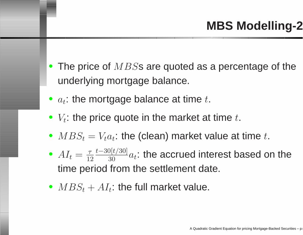
• The price of MBSs are quoted as a percentage of theunderlying mortgage balance.

• at: the mortgage balance at time t.

• Vt: the price quote in the market at time t.

• MBSt = Vtat: the (clean) market value at time t.

• AIt = τ12

t−30[t/30]30

at: the accrued interest based on thetime period from the settlement date.

• MBSt + AIt: the full market value.


MBS Modelling-3

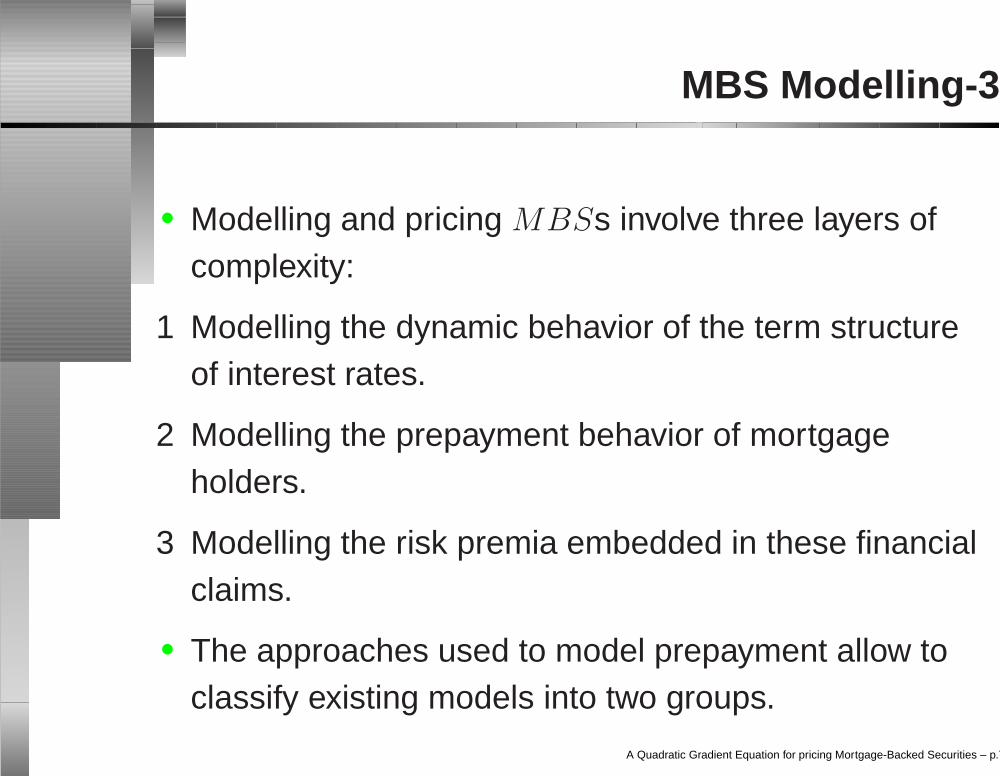
• Modelling and pricing MBSs involve three layers ofcomplexity:

1 Modelling the dynamic behavior of the term structureof interest rates.

2 Modelling the prepayment behavior of mortgageholders.

3 Modelling the risk premia embedded in these financialclaims.

• The approaches used to model prepayment allow toclassify existing models into two groups.


Prepayment Option

• The first type is related to American options, [Stanton,1995] and [Stanton & Wallace 2003].

• Paying off the loan is equivalent to exercising a calloption (V

p,t) on the underlying bond at, withtime-varying exercise price MB(t).

• The default option (V d,t) is an option to exchange one

asset (the house) for another (MB(t)).

• The mortgage liability is M t = at − V

p,t − V d,t.

• Borrowers choose when they prepay or default in orderto minimize the overall value M

t .


Prepayment Policy

• In a second class of models, the prepayment policyfollows a comparison between the prevailing mortgageand contract rates [Deng, Quigley, Van Order, 2000].

• This comparison can be measured using the differenceor a ratio of the two rates, and usually the 10 yearsTreasury yield is used as a proxy for the mortgage rate.


Prepayment Factors

• Xt = (X1t , . . . , XN

t ): the relevant economic factors.

• The MBS price at time t is Pt = P (Xt, t).

• The challenging task is to give a complete justificationto the choice of the market price of risk used to derivethe functional form of P .

• The model specification follows the work by X. Gabaixand O. Vigneron (1998).

• We characterized P as the unique solution of anonlinear parabolic partial differential equation, in aviscosity sense.


Cash-Flow

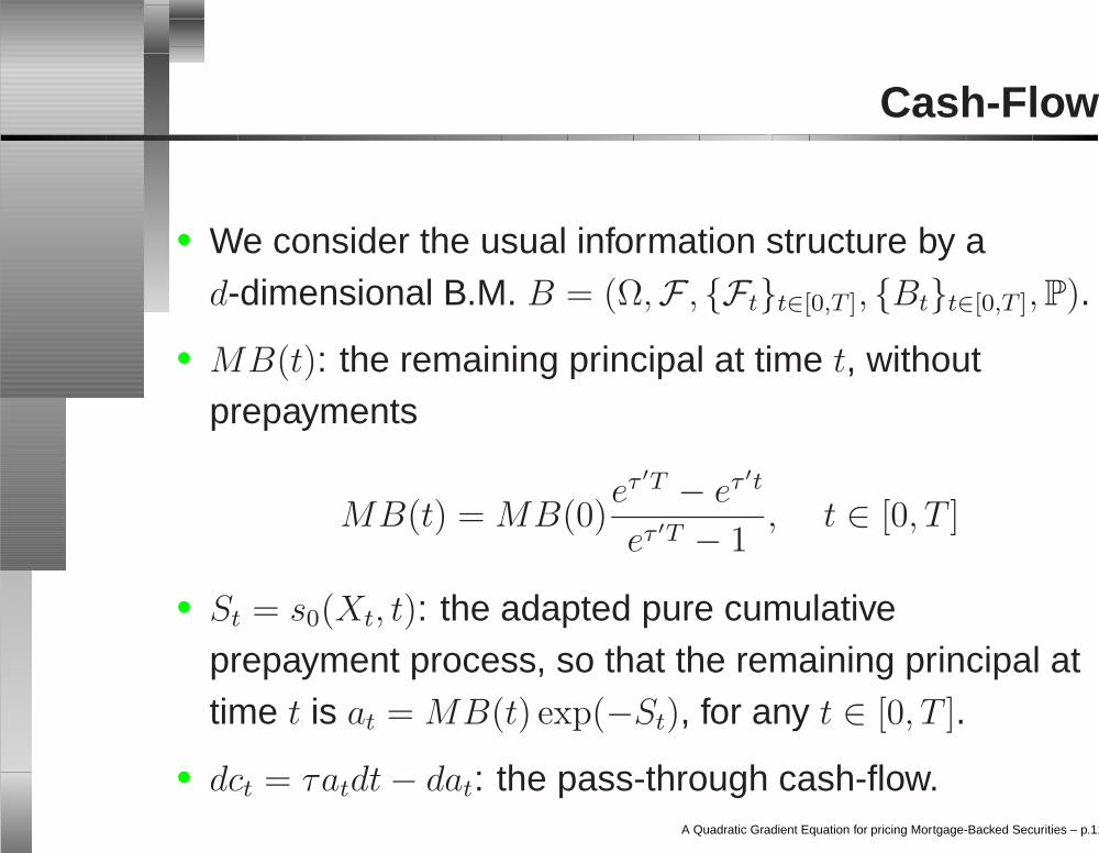
• We consider the usual information structure by ad-dimensional B.M. B = (Ω,F , Ftt∈[0,T ], Btt∈[0,T ], P).

• MB(t): the remaining principal at time t, withoutprepayments

MB(t) = MB(0)eτ ′T − eτ ′t

eτ ′T − 1, t ∈ [0, T ]

• St = s0(Xt, t): the adapted pure cumulativeprepayment process, so that the remaining principal attime t is at = MB(t) exp(−St), for any t ∈ [0, T ].

• dct = τatdt − dat: the pass-through cash-flow.A Quadratic Gradient Equation for pricing Mortgage-Backed Securities – p.11

Gain Process

• δ : Ω × [0, T ] → (0,∞) is an integrable discount rate.

• The economy is made up of a representative agent (atrader in the MBS market) with a risk aversion ρ > 0.

• dV Risklesst = δ(t)V Riskless

t dt, V Riskless0 = A0 > 0.

• Vt = (V Risklesst , V MBS,1

t , . . . , V MBS,kt ): the vector of asset

prices.

• GMBS,it = V MBS,i

t +∫ t

0dci

s, i = 1, . . . , k: the gain processof the asset i.

(A) The market is arbitrage-free and there exists a marketprice of risk γMBS

t = (γMBS,1t , . . . , γMBS,d

t ).A Quadratic Gradient Equation for pricing Mortgage-Backed Securities – p.12

Gain Volatility

• v ∈ L1,p ⇐⇒ |‖v‖|1,p < +∞.

|‖v‖|1,p =(‖v‖p

Lp(Ω×[0,T ]) + E

[‖Dv‖p

L2([0,T ]2)

])1/p

• From the generalized Clarke-Ocone formula (1991),we can prove a representation Theorem:

[Th(V)] Under (A), Sit ∈ D

2,1, DtSi ∈ L2(Ω × [0, T ]), for any

t ∈ [0, T ] and i = 1, . . . , k, γ = γMBS ∈ L1,4, σMBS,i

G (t) isgiven by:

−EQ

[∫ T

t

(τi − δ(s)

)e−

st δ(u)duai

s

(DtS

is +

∫ s

t

DtγudBu

)ds

∣∣∣Ft

]


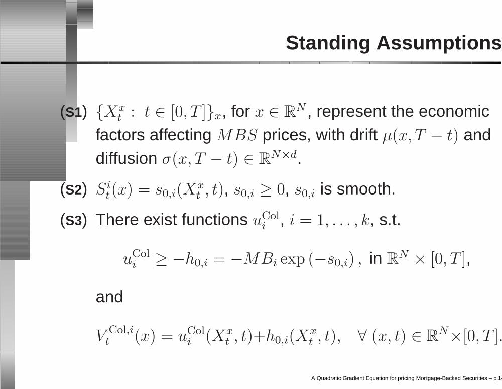
Standing Assumptions

(S1) Xxt : t ∈ [0, T ]x, for x ∈ R

N , represent the economicfactors affecting MBS prices, with drift µ(x, T − t) anddiffusion σ(x, T − t) ∈ R

N×d.

(S2) Sit(x) = s0,i(X

xt , t), s0,i ≥ 0, s0,i is smooth.

(S3) There exist functions uColi , i = 1, . . . , k, s.t.

uColi ≥ −h0,i = −MBi exp (−s0,i) , in R

N × [0, T ],

and

V Col,it (x) = uCol

i (Xxt , t)+h0,i(X

xt , t), ∀ (x, t) ∈ R

N×[0, T ].


An Equilibrium Model

• In MBS analysis, it seems natural to assume the m.p.r.to depend directly on the value of the liability.

• The liability to the mortgagor and the asset value to theinvestor differ only for a transaction cost, proportionalto at.

• Since a change of the borrower’s liability produces achange in the prepayment behavior, the proportionalitywith the asset value, yields a natural dependence ofthe m.p.r. on the MBS price (U ) and on its variation(∇xU ).


An Equilibrium Model-1

• x ∈ RN is the state of the economy.

• An equilibrium in the MBS market, is a d-dimensionalFt-adapted process γ(x), s.t.

1. dQ

dP= ξ

γ(x)T (Girsanov Exponential) is a risk-neutral

measure for the MBS Market;

2. [Th(V)] holds and

γt(x) = ρ

∑ki=1 σCol,i

G (t;x)∑ki=1 V Col,i

t (x) + V Risklesst

,

for every t ∈ [0, T ].



[Th.] Let γ(x) be an equilibrium. Under (S1)-(S3),uCol = (uCol

1 , . . . , uColk ) is a solution in R

N × (0, T ) of

ρ〈σ0 ∇ui,

∑kj=1 σ

0 ∇uj

V Risklesss +

∑kj=1[h0,j + uj]

〉 = −δ(s)(h0,i + ui)

+τih0,i + 〈∇ui, µ0〉 + ∂ui∂s

+ 12tr(σ0σ

0 ∇2ui),

ui(x, T ) = 0, i =, . . . , k.

σ0(x, s) = σ(x, T − s), µ0(x, s) = µ(x, T − s).

uColi (Xx

t , t) = EQ

[ ∫ T

t

(τi−δ(s)

)e−

st δ(u)duh0,i(X

xs , s)ds

∣∣∣Ft

].



[Th.] Assume (S1)-(S2). Let σ be bounded, and u = (u1,

. . . , uk) is a smooth solution of the system with ∇ui

bounded, ui + h0,i ≥ 0. For i =, . . . , k, define

V it ≡ ui(X

xt , t) + h0,i(X

xt , t)

Git ≡ V i

t +

∫ t

0

dcis.

Then (V Risklesst , G1

t , . . . , Gkt ) is an arbitrage-free market

which admits and equilibrium.


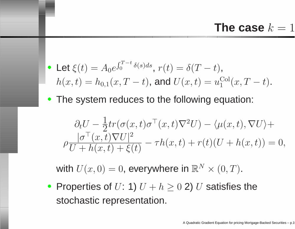
The case k = 1

• Let ξ(t) = A0e

T−t0 δ(s)ds, r(t) = δ(T − t),

h(x, t) = h0,1(x, T − t), and U(x, t) = uCol1 (x, T − t).

• The system reduces to the following equation:

∂tU − 12tr(σ(x, t)σ(x, t)∇2U) − 〈µ(x, t),∇U〉+

ρ|σ(x, t)∇U |2

U + h(x, t) + ξ(t)− τh(x, t) + r(t)(U + h(x, t)) = 0,

with U(x, 0) = 0, everywhere in RN × (0, T ).

• Properties of U : 1) U + h ≥ 0 2) U satisfies thestochastic representation.


Viscosity Solutions

[Def.] The parabolic 2-jet:P2,±u(x, t)=(∂tϕ(x, t),∇ϕ(x, t),∇2ϕ(x, t)) : u − ϕ hasa global strict max. (resp. min.) at (x, t).

[Def.] u : RN × [0, T ] → (a, b) l.b. and u.s.c. (resp. l.s.c.) is a

viscosity subsolution (resp. lower viscositysupersolution) if u(·, 0) ≤ u0(·), (resp. ≥ u0(·)), in R

N ,and for any (b, q, A) ∈ P2,±u(x, t)

b + F (x, t, u(x, t), q, A) ≤ 0 (resp. ≥ 0).

• Existence Results can be found in the User’s guide ofM.G. Crandall, H. Ishii, P.L. Lions (1992).


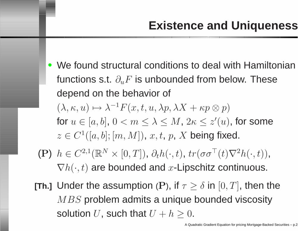
Existence and Uniqueness

• We found structural conditions to deal with Hamiltonianfunctions s.t. ∂uF is unbounded from below. Thesedepend on the behavior of(λ, κ, u) → λ−1F (x, t, u, λp, λX + κp ⊗ p)

for u ∈ [a, b], 0 < m ≤ λ ≤ M , 2κ ≤ z′(u), for somez ∈ C1([a, b]; [m,M ]), x, t, p, X being fixed.

(P) h ∈ C2,1(RN × [0, T ]), ∂th(·, t), tr(σσ(t)∇2h(·, t)),∇h(·, t) are bounded and x-Lipschitz continuous.

[Th.] Under the assumption (P), if τ ≥ δ in [0, T ], then theMBS problem admits a unique bounded viscositysolution U , such that U + h ≥ 0.


The Regularity-1

• The m.p. of prepayment risk is

γt(x) = ρσ(Xx

t , T − t)∇U(Xxt , T − t)

U(Xxt , T − t) + h(Xx

t , T − t) + ξ(T − t)

• The typical technique used to prove a representation ofU as an expectation, is based on the dynamicprogramming principle (Fleming & Soner, 1993).

• The existence of the value function is guaranteed bythe existence of the expected value.

• In the MBS model the expectation depends on U itself.Hence we need more regularity on ∇U .


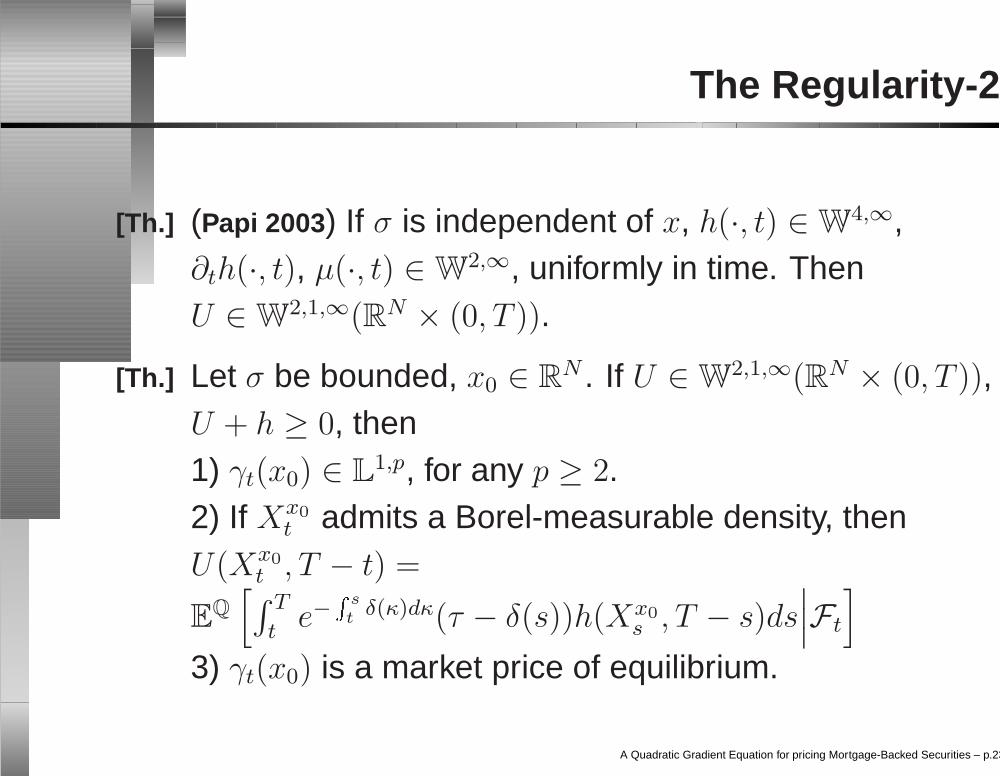
The Regularity-2

[Th.] (Papi 2003) If σ is independent of x, h(·, t) ∈ W4,∞,

∂th(·, t), µ(·, t) ∈ W2,∞, uniformly in time. Then

U ∈ W2,1,∞(RN × (0, T )).

[Th.] Let σ be bounded, x0 ∈ RN . If U ∈ W

2,1,∞(RN × (0, T )),U + h ≥ 0, then1) γt(x0) ∈ L

1,p, for any p ≥ 2.2) If Xx0

t admits a Borel-measurable density, thenU(Xx0

t , T − t) =

EQ

[∫ T

te−

st δ(κ)dκ(τ − δ(s))h(Xx0

s , T − s)ds∣∣∣Ft

]3) γt(x0) is a market price of equilibrium.


Path Dependency

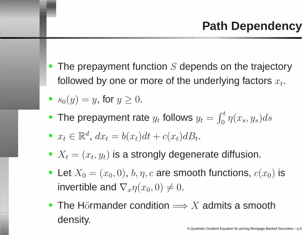
• The prepayment function S depends on the trajectoryfollowed by one or more of the underlying factors xt.

• s0(y) = y, for y ≥ 0.

• The prepayment rate yt follows yt =∫ t

0η(xs, ys)ds

• xt ∈ Rd, dxt = b(xt)dt + c(xt)dBt.

• Xt = (xt, yt) is a strongly degenerate diffusion.

• Let X0 = (x0, 0), b, η, c are smooth functions, c(x0) isinvertible and ∇xη(x0, 0) = 0.

• The Hormander condition =⇒ X admits a smoothdensity.


References

• M. Papi, A Generalized Osgood Condition for ViscositySolutions to Fully Nonlinear Parabolic DegenerateEquations, Adv. Differential Equations, 7 (2002),1125-1151.

• M. Papi, Regularity Results for a Class of SemilinearParabolic Degenerate Equations and Applications,Comm. Math. Sci., 1 (2003), 229-244.

• M.Papi, M.Briani. A PDE-based approach for pricingMortgage-Backed Securities, Preprint Luiss 2004.


Documents

A Quadratic Gradient Equation for pricing Mortgage-Backed Securities