Embed Size (px)
Citation preview
HAL Id: hal-01243467https://hal.univ-reunion.fr/hal-01243467
Submitted on 12 Jun 2018
HAL is a multi-disciplinary open accessarchive for the deposit and dissemination of sci-entific research documents, whether they are pub-lished or not. The documents may come fromteaching and research institutions in France orabroad, or from public or private research centers.
L’archive ouverte pluridisciplinaire HAL, estdestinée au dépôt et à la diffusion de documentsscientifiques de niveau recherche, publiés ou non,émanant des établissements d’enseignement et derecherche français ou étrangers, des laboratoirespublics ou privés.
A proposal for social pricing of water supply in Côted’Ivoire
Daouda Diakité, Aggey Semenov, Alban Thomas
To cite this version:Daouda Diakité, Aggey Semenov, Alban Thomas. A proposal for social pricing of water sup-ply in Côte d’Ivoire. Journal of Development Economics, Elsevier, 2009, 88 (2), pp.258–268.�10.1016/j.jdeveco.2008.03.003�. �hal-01243467�
A Proposal for Social Pricing of Water Supply in Cote
d’Ivoire∗
Daouda DIAKITE†, Aggey SEMENOV‡and Alban THOMAS§
February 2008
Abstract
We consider the design of a nonlinear social tariff for residential water in Cote
d’Ivoire, which is a case of a monopolistic private operator supplying a population
of heterogeneous consumers. The proposed optimal tariff includes an initial “social”
block with a low unit price, and higher consumption blocks with a monopoly pricing
rule. This optimal nonlinear tariff is calibrated using econometric estimates of a panel-
data residential water demand equation. Welfare changes associated with moving from
the actual tariff to approximations of the optimal pricing system are computed under
different tariff scenarios. We find that gains in consumer welfare would outweigh losses
in producer surplus in a majority of Ivorian local communities.
Keys Words : Multiblock tariff, Social Pricing, Residential Water Supply.
JEL classification codes: C33, I38, O13, Q25.
∗ We are grateful to Mark Rosenzweig (the Editor), four anonymous referees, Robert Wilson and Michael
Hanemann for helpful comments.†Toulouse School of Economics, LERNA.‡National University of Singapore.§Corresponding author. Toulouse School of Economics, INRA, LERNA. 21 Allee de Brienne, F-31000
Toulouse, France. email [email protected]
1
1 Introduction
Over the past 20 years, the world’s residential water consumption has increased at a much
higher rate than that of population. The international community has become progressively
aware of the role played by access to safe drinking water and sewage in economic development.
Indeed, the vast majority of households without such access are in developing countries,
where the problem often does not lie with the scarcity of water, but with the difficulty
to finance water supply and treatment operations. Investments in the water industry are
typically long-term, due to large infrastructure costs associated with redesigning or building
water networks.
As governments in developing countries find it challenging to fund these investment re-
quirements, an alternative is to promote public-private partnerships or concession contracts
in the water industry. Resorting to private companies to invest and operate water utilities
does not mean that the objectives of the local communities and the State regarding environ-
mental protection and consumers’ welfare will be neglected. As it stands, private companies
operating in developing countries face difficulties in meeting their financial objectives, be-
cause a fraction of the consumers fail to pay their water bills. Majority of customers are
typically able to pay their daily water residential consumption as the marginal water prices
are generally low. However, for operators, fixed costs make a significant share of water bills
and often lead to difficulties in cost recovery.1
One of the possibilities to facilitate water access to poor households is to design an
income-targeted subsidy policy. Under such a system, a household, after being identified as
“poor”, pays only a fraction of the full water bill or part of the fixed fee (i.e., the lump-
sum payment corresponding to the connection fee). The operator is then compensated by
a transfer from the local community, or from the federal or regional compensation schemes.
Another possibility is to base the subsidy policy on volumes consumed only. In this case, a
multi-part block rate tariff is designed, with a minimum water consumption level supplied
1This is particularly true for some countries in Central America and Africa (see Strand and Walker, 2005;
Collignon et al., 2000).
2
at zero or very low price. The losses for the operator are compensated from the higher
consumption blocks and/or from other customer categories, for instance, the industries.
Such initiatives, called “social pricing”, are followed in various regions around the world,
and have shown that different solutions require careful adjustments to suit local population
needs. Social tariff schemes rely on several tariff components as instruments for modifying
the households’ behavior, in particular the structure of the consumption blocks and their
associated unit prices, and/or the fixed part of the tariff. From a theoretical point of view,
the optimal social pricing scheme should take into account consumers’ preferences for water
consumption along with the preferences of the regulator. The latter is assumed to maximize
consumer welfare while ensuring a profitable operation for the private company in charge of
the water network.
In this paper we suggest a simple social tariff structure for a monopolistic operator
supplying a population of income-diverse consumers. The optimal pricing rule is obtained
as the solution to a special case of the general Ramsey pricing problem presented in Wilson
(1993). Under the Ramsey pricing model, the initial level of consumption is charged at a
fixed rate, up to a level with is determined by the parameters of the model. While Wilson
(1993) interprets this multi-part tariff in the context of fixed fee (access fee for instance),
in our case the first pricing block of the tariff originates from the social objective of the
regulator.
The contribution of the present paper to the literature on nonlinear pricing does not lie in
the construction of a new framework for designing optimal tariffs for public services, rather,
by using Wilson’s (1993) theoretical framework of nonlinear pricing, we propose a method
for calibrating and approximating (by multi-block price systems) optimal tariffs that include
social considerations.
The water industry in Cote d’Ivoire presents an interestring case for several reasons.
First, a common rate policy for every local community of the country is implemented by the
(sole) water operator SODECI (Societe de Distribution d’Eau de Cote d’Ivoire, established
in 1956). Second, poor customers actually benefit from subsidized connection charges, as
3
well as from a reduced-rate initial consumption block. Third, the existing tariff is of the
increasing-block type, which means that higher-income customers would also benefit from
the reduced-rate in the initial consumption block.
By comparing the optimal nonlinear tariff with the existing tariff in Cote d’Ivoire, we
determine whether an increase in social welfare could be achieved by modifying the number
of consumption blocks, their threshold levels and unit prices. In particular, we examine the
impact on social welfare of increasing the number of block rates. To this end, we replace our
optimal pricing system with a series of multiple-rate tariff approximations, that are simplified
for the sake of clarity. Although this comes at the cost of losing optimality properties of
the tariff, such approximations are more in line with the apparent features of the existing
tariffs. We also examine the impact on social welfare of imposing a water tariff that has
the increasing block structure, although the optimal pricing rule is not monotonic in water
volumes.
The paper is organized as follows. Section 2 discusses water pricing and describes the
existing pricing scheme in Cote d’Ivoire. Section 3 presents a theoretical motivation for
nonlinear social pricing. Section 4 presents an empirical application to Cote d’Ivoire. The
results from the simulation experiment are given in Section 5, and a comparison is made with
the existing water tariff scheme in Cote d’Ivoire. We consider several approximations to the
optimal water tariff by imposing an increasing block rate tariff structure and by letting the
number of pricing blocks vary. Section 6 concludes.
2 Water pricing
2.1 Pricing rules for water utilities
Whether publicly or privately operated, water utilities are generally considered natural mo-
nopolies because of declining long-run average costs, and high fixed costs relative to variable
costs. Designing an efficient water pricing policy is crucial for water companies in local com-
munities. A price policy is often a compromise between various (and possibly conflicting)
4
objectives: economic efficiency, cost recovery, equity, and resource conservation.
The first objective of a water utility pricing scheme is to generate revenues covering at
least the operating (short-run) costs. Without regulation, a monopoly maximizes profit so
that the marginal cost is equal to the marginal revenue. By doing so however, consumers’
surplus is minimized which results in a socially suboptimal tariff. If the monopoly is regulated
by an utilitarian social planner, maximizing the social welfare leads to the marginal cost
pricing rule (MCP) and thus, satisfying the economic efficiency objective. If price does not
reflect the social marginal cost, consumers do not receive appropriate information about
the societal cost of a marginal increase in demand (Renzetti and Kushner, 2004). MCP
has received a criticism on the account of absence of a budget constraint, deficit if the firm
operates under increasing returns to scale, etc. Further, it has given rise to a number of
practical difficulties (Boland and Whittington, 2000). Also, from an equity point of view,
MCP collects too much revenue if the marginal cost is above the average cost. For these
reasons, there is little evidence of real-world applications of MCP in water utilities (Renzetti,
2000).
An alternative solution is to use a two-part tariff with a marginal price corresponding to
the marginal cost and a fixed charge allowing for the deficit recovery. However, this system is
often seen as regressive as the high connection fee constitutes a significant proportion of the
total bill for low-volume consumers (and therefore, a significant proportion of the average
water price).2 If the water managers are concerned with the distributional consequences of
the tariff, then a preferred policy is to set the unit charge above the marginal cost, so as
to reduce the fixed part of the tariff. Renzetti (2000) shows that such a policy (also called
the Feldstein pricing) is clearly suboptimal in a wide range of cases as the unit rates are
significantly distorted from the marginal cost.
A natural extension of the two-part tariff is the class of block rate pricing systems, the
Increasing Block Rate (IBR) or the Decreasing Block Rate (DBR), in which the number
2Average price in the two-part tariff is equal to the marginal price plus the fixed charge divided by the
consumption volume.
5
of blocks is greater than two.3 Increasing or decreasing block rate pricing can solve the
problem of excess profits and losses generated by the marginal pricing in cases of economies
and diseconomies of scale respectively. One drawback of the block rate pricing is that
it makes the revenue of the water utility more variable as consumers, by changing their
water consumption may switch from one price block to another. Nowadays, the use of the
IBR systems is widespread in developing countries (Boland and Whittington, 2000), their
success lies in the objectives they are claimed to achieve: the equity objective by subsidizing
small (presumably poor) customers by charging bigger customers, the resource conservation
objective, the promotion of economic efficiency through the marginal cost pricing for the
highest block. However, the IBR pricing may be in contradiction with the basic principles of
monopoly pricing. It may even lead to social losses when the block rates are not designed to
preserve the interests of the water operator and large consumers. Some water companies use
more complex pricing schemes that combine both the increasing and the decreasing block
structures. The marginal price can increase in the first block and then decrease to favor both
very small and very large water consumers.
In a second-best world, where the budget constraint of the water utility is introduced, the
pricing system involves the Ramsey-Boiteux rule (see, e.g., Laffont and Tirole, 2000; Prieger,
1996; Baumol, 1987). In this case, the gap between the marginal price and the marginal cost
depends on the price elasticity of water demand and the cost of the budget constraint, and
this pricing rule ensures the highest social welfare under a budget constraint. In practice,
implementing this policy requires perfect knowledge of the production cost and consumer
demand function for a private monopoly, and of the consumer demand function for a public
monopoly.
Extensions of the single price models such as the MCP or the Ramsey-Boiteux pricing
involve a nonlinear pricing schedule (Brown and Sibley, 1986; Wilson, 1993), for a welfare-
maximizing public utility faced with a set of income-diverse consumers. Consumers vary
3Boland and Whitthington (2000) proposed a uniform price with rebate as an alternative to a two-part
tariff.
6
according to their “type” which is represented by an unobservable parameter θ (e.g., the
price sensitivity of demand, income). The price schedule is a nonlinear function of quantity
(either increasing or decreasing in the consumption level), and depends on both supply and
demand parameters (in particular, the utility’s marginal cost and the distribution of θ).
The practical implementation of an optimal nonlinear pricing rule involves the use of an
approximation by blocks, for instance, using the IBR system. In this case, the nonlinear
price formula is discretized into a number of blocks, so as to mimic the original nonlinear
pricing rule. A way to reduce the loss in optimality due to approximation is to consider a
large number of blocks in the tariff.
2.2 Water pricing in Cote d’Ivoire
In Cote d’Ivoire, the water supply sector is divided into two subsectors: urban water sup-
ply systems (named “hydraulique urbaine”) and rural water supply (named “hydraulique
villageoise”). This distinction is based on technical network and connection parameters,
investments, financing and operating modes, and the type of population supplied. For ex-
ample, a water supply system is considered urban if the local community’s population is
above 3 000 inhabitants, if a water distribution network exists, etc. 4
Since the 1987 delegation contract, the concession of SODECI - the largest water oper-
ator in the country, caters only to communities in the urban water supply systems. Other
communities - according to criteria mentioned above - are supplied by the rural water sys-
tems, which could be either traditional (hand-pumps) or improved systems (water towers
and standpipes).
As in most countries in Western Africa, SODECI uses an IBR pricing scheme. The water
tariff includes a value added tax and two special taxes for financing the Fonds National de
l’eau (FNE, National Water Fund) and the Fonds de Developpement (FDE, Development
Fund for Water) respectively. The FDE is devoted to financing “social” (subsidized) network
connections, hydraulic facility replacement costs, network extension operations and invest-
4See Direction de l’Hydraulique Humaine (2001) for a description of these criteria.
7
ments in new facilities and equipment; while the FNE is concerned with the contract-related
loans in the water sector.
The price components to be used by SODECI are specified in the 1987 contract and
a price revision should occur every 5 years according to the contract. In fact, the price
structure has experienced a series of modifications over the period 1996-2005.
The first block, called “forfait”(set price), concerns volumes below 36 m3/year, where
households pay a fixed fee of 16.07 USD/year.5 The second block, called “social”, is for
volumes between 36 and 76 m3/year and has a unit price of 0.50 USD / m3. The third
block, called “domestic”, is for volumes between 76 and 364 m3/year and has a flat rate of
0.79 USD / m3. The final block, denoted “standard”, concerns volumes above 364 m3/year
and is associated with a unit price of 1.26 USD / m3. The average annual household con-
sumption is around 120 m3, therefore a significant proportion of the total volumes consumed
by households is expected to lie within the third block. Finally, note that the “social” block6
more or less follows standard recommendations in terms of basic needs, namely a minimum
requirement of 76 m3/year corresponding to a 5-person household (see Gleick, 1996).7
In order to increase the supply of residential drinking water, the authority in charge
of urban water services had formulated an ambitious policy of subsidized residential water
connections in the mid 1980s. The subsidy was granted to 15 mm-diameter water pipe con-
nections (this was done to limit the available volume for the household requirements) within
a 12 meter limit from the main connection pipe to the water meter (in the public domain).
Above this limit, any additional pipe connection cost as well as the costs of the appliances
after the meter were borne by the residential customer. The policy benefited customers from
a lower connection cost of 36.68 USD instead of 359 USD for a usual connection. SODECI
5In this paper, monetary amounts are expressed in US Dollars. 1 USD is about 656 FCFA (monetary
unit of the African French-Speaking Financial Community).6The social block included the “forfait” block. Note that the first and second block have the same unit
price of 0.44 USD per m3. The first block was designed to take into account very small users.7In Cote d’Ivoire, households have on average 6.5 members. The minimum individual requirement is 15
m3 /year.
8
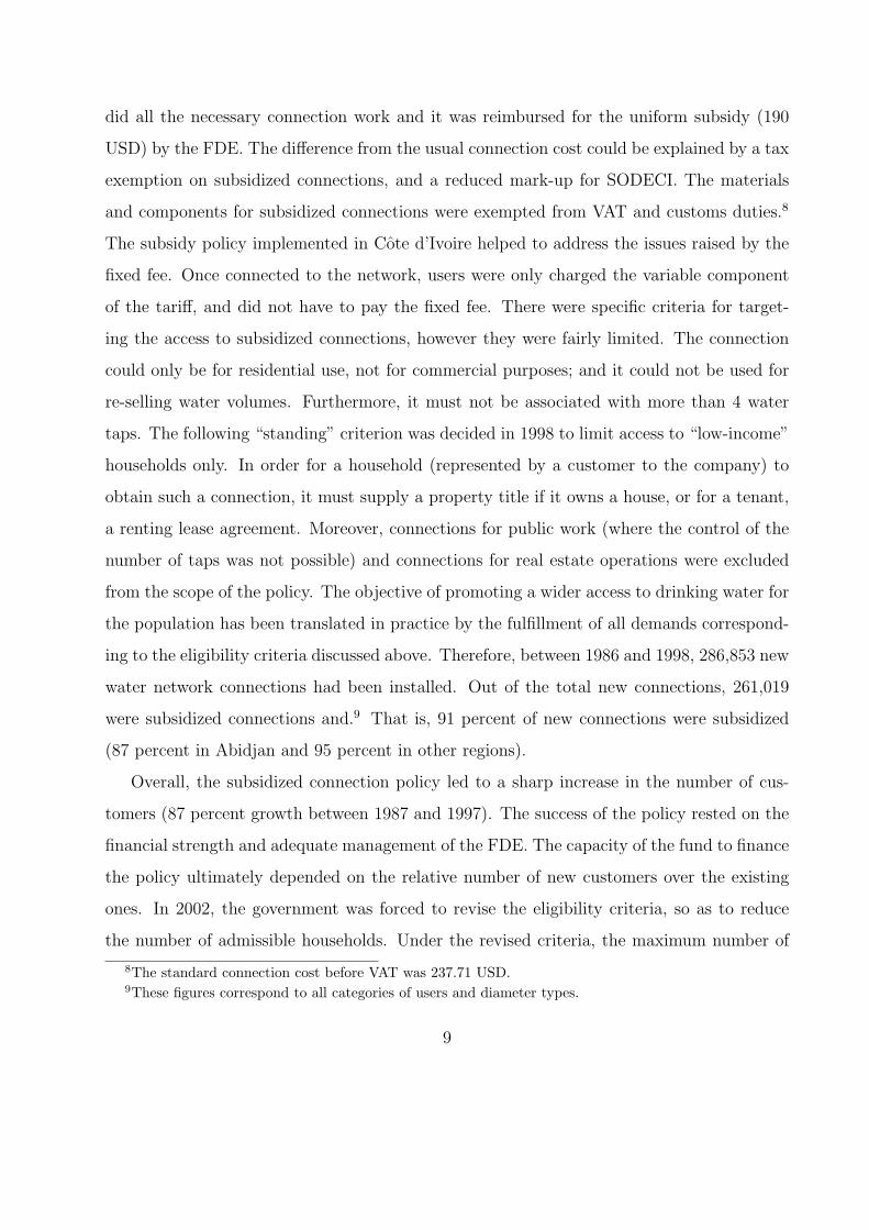
did all the necessary connection work and it was reimbursed for the uniform subsidy (190
USD) by the FDE. The difference from the usual connection cost could be explained by a tax
exemption on subsidized connections, and a reduced mark-up for SODECI. The materials
and components for subsidized connections were exempted from VAT and customs duties.8
The subsidy policy implemented in Cote d’Ivoire helped to address the issues raised by the
fixed fee. Once connected to the network, users were only charged the variable component
of the tariff, and did not have to pay the fixed fee. There were specific criteria for target-
ing the access to subsidized connections, however they were fairly limited. The connection
could only be for residential use, not for commercial purposes; and it could not be used for
re-selling water volumes. Furthermore, it must not be associated with more than 4 water
taps. The following “standing” criterion was decided in 1998 to limit access to “low-income”
households only. In order for a household (represented by a customer to the company) to
obtain such a connection, it must supply a property title if it owns a house, or for a tenant,
a renting lease agreement. Moreover, connections for public work (where the control of the
number of taps was not possible) and connections for real estate operations were excluded
from the scope of the policy. The objective of promoting a wider access to drinking water for
the population has been translated in practice by the fulfillment of all demands correspond-
ing to the eligibility criteria discussed above. Therefore, between 1986 and 1998, 286,853 new
water network connections had been installed. Out of the total new connections, 261,019
were subsidized connections and.9 That is, 91 percent of new connections were subsidized
(87 percent in Abidjan and 95 percent in other regions).
Overall, the subsidized connection policy led to a sharp increase in the number of cus-
tomers (87 percent growth between 1987 and 1997). The success of the policy rested on the
financial strength and adequate management of the FDE. The capacity of the fund to finance
the policy ultimately depended on the relative number of new customers over the existing
ones. In 2002, the government was forced to revise the eligibility criteria, so as to reduce
the number of admissible households. Under the revised criteria, the maximum number of
8The standard connection cost before VAT was 237.71 USD.9These figures correspond to all categories of users and diameter types.
9
water taps associated with the residential connection must not exceed 3. Furthermore, a
single connection could only be made in a housing unit, and the total number of subsidized
connections every year could not exceed 10,000 for the whole country.
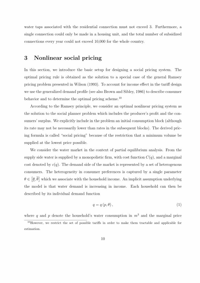
3 Nonlinear social pricing
In this section, we introduce the basic setup for designing a social pricing system. The
optimal pricing rule is obtained as the solution to a special case of the general Ramsey
pricing problem presented in Wilson (1993). To account for income effect in the tariff design
we use the generalized demand profile (see also Brown and Sibley, 1986) to describe consumer
behavior and to determine the optimal pricing scheme.10
According to the Ramsey principle, we consider an optimal nonlinear pricing system as
the solution to the social planner problem which includes the producer’s profit and the con-
sumers’ surplus. We explicitly include in the problem an initial consumption block (although
its rate may not be necessarily lower than rates in the subsequent blocks). The derived pric-
ing formula is called “social pricing” because of the restriction that a minimum volume be
supplied at the lowest price possible.
We consider the water market in the context of partial equilibrium analysis. From the
supply side water is supplied by a monopolistic firm, with cost function C(q), and a marginal
cost denoted by c(q). The demand side of the market is represented by a set of heterogenous
consumers. The heterogeneity in consumer preferences is captured by a single parameter
θ ∈[θ, θ]
which we associate with the household income. An implicit assumption underlying
the model is that water demand is increasing in income. Each household can then be
described by its individual demand function
q = q (p, θ) , (1)
where q and p denote the household’s water consumption in m3 and the marginal price
10However, we restrict the set of possible tariffs in order to make them tractable and applicable for
estimation.
10
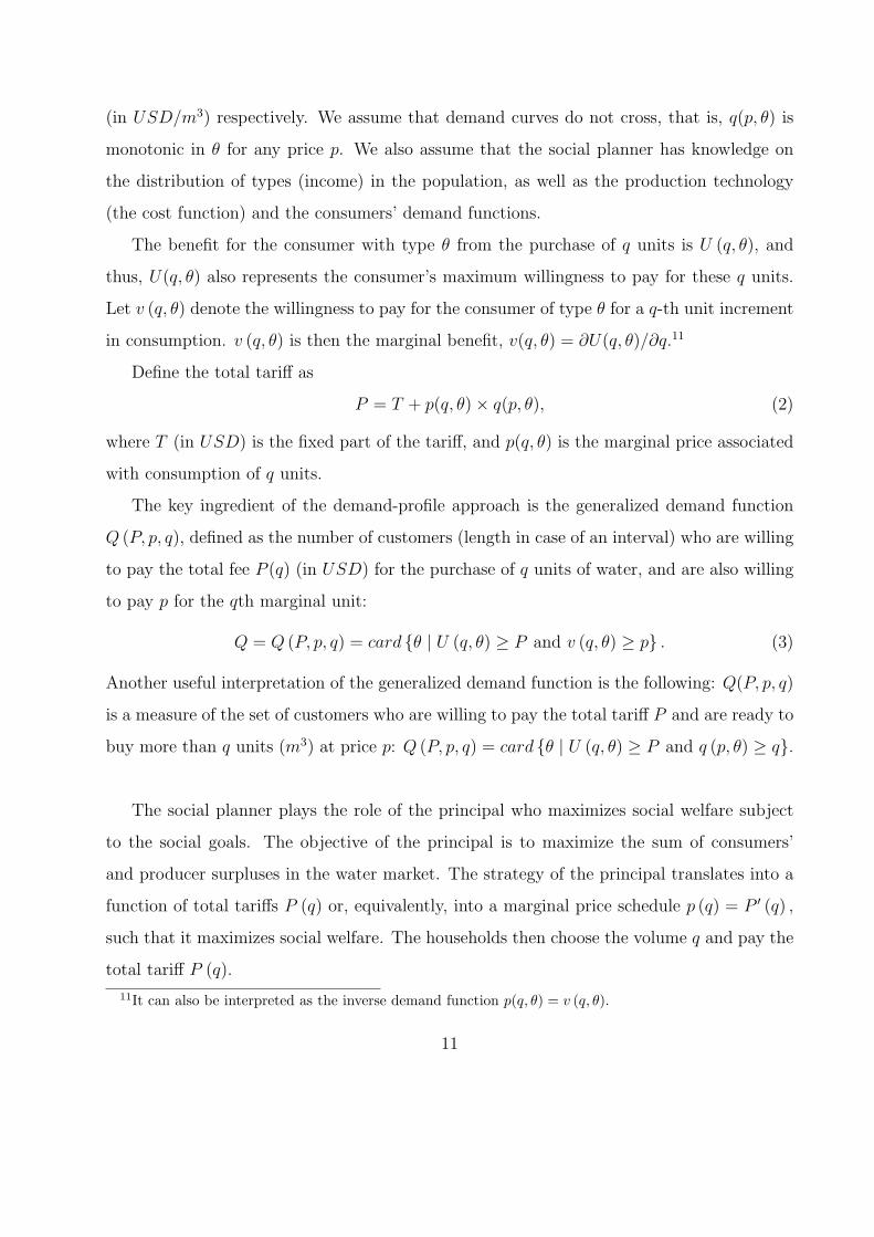
(in USD/m3) respectively. We assume that demand curves do not cross, that is, q(p, θ) is
monotonic in θ for any price p. We also assume that the social planner has knowledge on
the distribution of types (income) in the population, as well as the production technology
(the cost function) and the consumers’ demand functions.
The benefit for the consumer with type θ from the purchase of q units is U (q, θ), and
thus, U(q, θ) also represents the consumer’s maximum willingness to pay for these q units.
Let v (q, θ) denote the willingness to pay for the consumer of type θ for a q-th unit increment
in consumption. v (q, θ) is then the marginal benefit, v(q, θ) = ∂U(q, θ)/∂q.11
Define the total tariff as
P = T + p(q, θ)× q(p, θ), (2)
where T (in USD) is the fixed part of the tariff, and p(q, θ) is the marginal price associated
with consumption of q units.
The key ingredient of the demand-profile approach is the generalized demand function
Q (P, p, q), defined as the number of customers (length in case of an interval) who are willing
to pay the total fee P (q) (in USD) for the purchase of q units of water, and are also willing
to pay p for the qth marginal unit:
Q = Q (P, p, q) = card {θ | U (q, θ) ≥ P and v (q, θ) ≥ p} . (3)
Another useful interpretation of the generalized demand function is the following: Q(P, p, q)
is a measure of the set of customers who are willing to pay the total tariff P and are ready to
buy more than q units (m3) at price p: Q (P, p, q) = card {θ | U (q, θ) ≥ P and q (p, θ) ≥ q}.
The social planner plays the role of the principal who maximizes social welfare subject
to the social goals. The objective of the principal is to maximize the sum of consumers’
and producer surpluses in the water market. The strategy of the principal translates into a
function of total tariffs P (q) or, equivalently, into a marginal price schedule p (q) = P ′ (q) ,
such that it maximizes social welfare. The households then choose the volume q and pay the
total tariff P (q).
11It can also be interpreted as the inverse demand function p(q, θ) = v (q, θ).
11
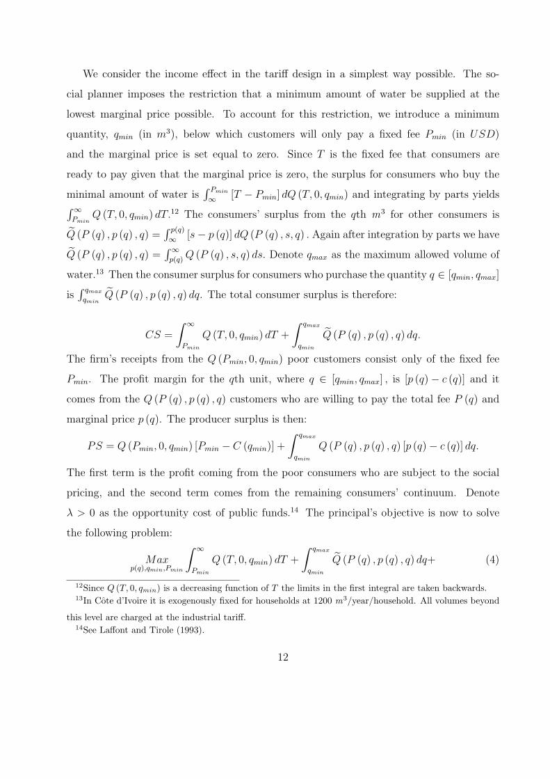
We consider the income effect in the tariff design in a simplest way possible. The so-
cial planner imposes the restriction that a minimum amount of water be supplied at the
lowest marginal price possible. To account for this restriction, we introduce a minimum
quantity, qmin (in m3), below which customers will only pay a fixed fee Pmin (in USD)
and the marginal price is set equal to zero. Since T is the fixed fee that consumers are
ready to pay given that the marginal price is zero, the surplus for consumers who buy the
minimal amount of water is∫ Pmin
∞ [T − Pmin] dQ (T, 0, qmin) and integrating by parts yields∫∞Pmin
Q (T, 0, qmin) dT.12 The consumers’ surplus from the qth m3 for other consumers is
Q (P (q) , p (q) , q) =∫ p(q)
∞ [s− p (q)] dQ (P (q) , s, q) . Again after integration by parts we have
Q (P (q) , p (q) , q) =∫∞
p(q)Q (P (q) , s, q) ds. Denote qmax as the maximum allowed volume of
water.13 Then the consumer surplus for consumers who purchase the quantity q ∈ [qmin, qmax]
is∫ qmax
qminQ (P (q) , p (q) , q) dq. The total consumer surplus is therefore:
CS =
∫ ∞
Pmin
Q (T, 0, qmin) dT +
∫ qmax
qmin
Q (P (q) , p (q) , q) dq.
The firm’s receipts from the Q (Pmin, 0, qmin) poor customers consist only of the fixed fee
Pmin. The profit margin for the qth unit, where q ∈ [qmin, qmax] , is [p (q)− c (q)] and it
comes from the Q (P (q) , p (q) , q) customers who are willing to pay the total fee P (q) and
marginal price p (q). The producer surplus is then:
PS = Q (Pmin, 0, qmin) [Pmin − C (qmin)] +
∫ qmax
qmin
Q (P (q) , p (q) , q) [p (q)− c (q)] dq.
The first term is the profit coming from the poor consumers who are subject to the social
pricing, and the second term comes from the remaining consumers’ continuum. Denote
λ > 0 as the opportunity cost of public funds.14 The principal’s objective is now to solve
the following problem:
Maxp(q),qmin,Pmin
∫ ∞
Pmin
Q (T, 0, qmin) dT +
∫ qmax
qmin
Q (P (q) , p (q) , q) dq+ (4)
12Since Q (T, 0, qmin) is a decreasing function of T the limits in the first integral are taken backwards.13In Cote d’Ivoire it is exogenously fixed for households at 1200 m3/year/household. All volumes beyond
this level are charged at the industrial tariff.14See Laffont and Tirole (1993).
12
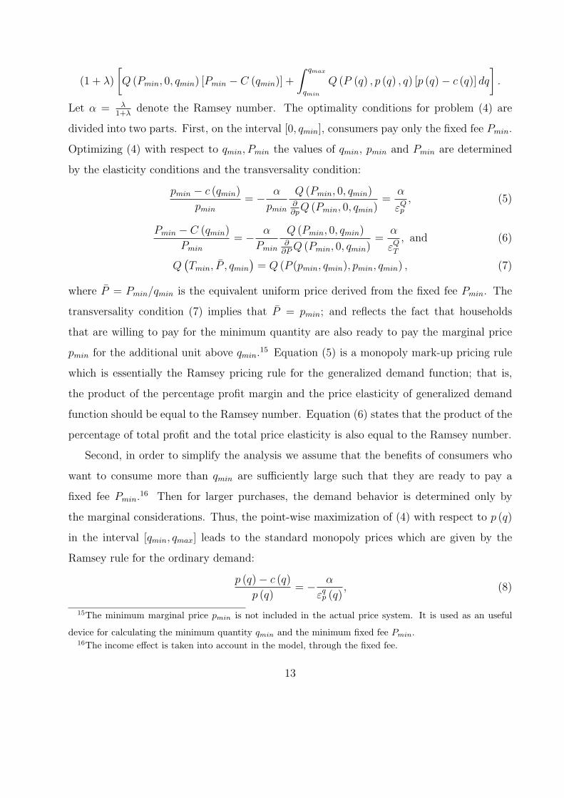
(1 + λ)
[Q (Pmin, 0, qmin) [Pmin − C (qmin)] +
∫ qmax
qmin
Q (P (q) , p (q) , q) [p (q)− c (q)] dq
].
Let α = λ1+λ
denote the Ramsey number. The optimality conditions for problem (4) are
divided into two parts. First, on the interval [0, qmin], consumers pay only the fixed fee Pmin.
Optimizing (4) with respect to qmin, Pmin the values of qmin, pmin and Pmin are determined
by the elasticity conditions and the transversality condition:
pmin − c (qmin)
pmin
= − α
pmin
Q (Pmin, 0, qmin)∂∂p
Q (Pmin, 0, qmin)=
α
εQp
, (5)
Pmin − C (qmin)
Pmin
= − α
Pmin
Q (Pmin, 0, qmin)∂
∂PQ (Pmin, 0, qmin)
=α
εQT
, and (6)
Q(Tmin, P , qmin
)= Q (P (pmin, qmin), pmin, qmin) , (7)
where P = Pmin/qmin is the equivalent uniform price derived from the fixed fee Pmin. The
transversality condition (7) implies that P = pmin; and reflects the fact that households
that are willing to pay for the minimum quantity are also ready to pay the marginal price
pmin for the additional unit above qmin.15 Equation (5) is a monopoly mark-up pricing rule
which is essentially the Ramsey pricing rule for the generalized demand function; that is,
the product of the percentage profit margin and the price elasticity of generalized demand
function should be equal to the Ramsey number. Equation (6) states that the product of the
percentage of total profit and the total price elasticity is also equal to the Ramsey number.
Second, in order to simplify the analysis we assume that the benefits of consumers who
want to consume more than qmin are sufficiently large such that they are ready to pay a
fixed fee Pmin.16 Then for larger purchases, the demand behavior is determined only by
the marginal considerations. Thus, the point-wise maximization of (4) with respect to p (q)
in the interval [qmin, qmax] leads to the standard monopoly prices which are given by the
Ramsey rule for the ordinary demand:
p (q)− c (q)
p (q)= − α
εqp (q)
, (8)
15The minimum marginal price pmin is not included in the actual price system. It is used as an useful
device for calculating the minimum quantity qmin and the minimum fixed fee Pmin.16The income effect is taken into account in the model, through the fixed fee.
13
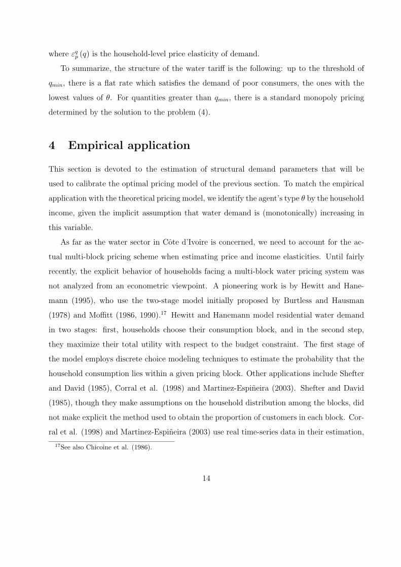
where εqp (q) is the household-level price elasticity of demand.
To summarize, the structure of the water tariff is the following: up to the threshold of
qmin, there is a flat rate which satisfies the demand of poor consumers, the ones with the
lowest values of θ. For quantities greater than qmin, there is a standard monopoly pricing
determined by the solution to the problem (4).
4 Empirical application
This section is devoted to the estimation of structural demand parameters that will be
used to calibrate the optimal pricing model of the previous section. To match the empirical
application with the theoretical pricing model, we identify the agent’s type θ by the household
income, given the implicit assumption that water demand is (monotonically) increasing in
this variable.
As far as the water sector in Cote d’Ivoire is concerned, we need to account for the ac-
tual multi-block pricing scheme when estimating price and income elasticities. Until fairly
recently, the explicit behavior of households facing a multi-block water pricing system was
not analyzed from an econometric viewpoint. A pioneering work is by Hewitt and Hane-
mann (1995), who use the two-stage model initially proposed by Burtless and Hausman
(1978) and Moffitt (1986, 1990).17 Hewitt and Hanemann model residential water demand
in two stages: first, households choose their consumption block, and in the second step,
they maximize their total utility with respect to the budget constraint. The first stage of
the model employs discrete choice modeling techniques to estimate the probability that the
household consumption lies within a given pricing block. Other applications include Shefter
and David (1985), Corral et al. (1998) and Martinez-Espineira (2003). Shefter and David
(1985), though they make assumptions on the household distribution among the blocks, did
not make explicit the method used to obtain the proportion of customers in each block. Cor-
ral et al. (1998) and Martinez-Espineira (2003) use real time-series data in their estimation,
17See also Chicoine et al. (1986).
14

but the data were available for a limited number of local communities only. In practice,
when working with aggregate data at the municipality level, the number of customers in the
different pricing blocks is rarely available for each community. Since the water tariff in Cote
d’Ivoire is of the multi-block type, we will largely use the estimation techniques for such
pricing described in the last two studies mentioned above.
The data are collected directly from SODECI, for 156 local communities over the years
1998-2002, the total number of observations in the panel is 780. These communities are
selected because they are already connected to the SODECI water network before 1998.18
In each local community, the pricing scheme is the same, with three blocks associated
with three different marginal prices19. Table 1 presents descriptive statistics for the aver-
age water consumption (per household), block shares s, average price over the three pricing
blocks, and household income. We can see that block 2 accounts for more than 50 percent
of the total water consumption, whereas block 3 has a low number of customers on average
(8 percent). We also report statistics for demand and block-choice explanatory variables: I
(income, in million FCFA), UNPAID (unpaid volumes per household in m3), PUNPAID
(proportion of unpaid volumes, that is, unpaid volumes divided by total water volume billed
to customers), NEWSUB (proportion of subsidized new customers), RETURN (water net-
work rate of return), CUST (number of connections in the local community), and ACCESS
(access to water in 1000 individuals, CUST multiplied by the size of the household).
[TABLE 1 ABOUT HERE]
As shown in Corral et al. (1998), the estimating equation for water demand at the
community level is:
qjt = β0 + β1
(m∑
i=1
sijtpijt
)+ β2
(m∑
i=1
sijt(Ijt − dij)
)+ δZjt + εjt, (9)
18For these communities, database are available from SODECI and Direction de l’hydraulique humaine
(the regulation authority of the sector). For other communities not included in the SODECI supply area,
there is no water operator and a village committee directly manages the system. So the data are not available
for such communities (and additional data collection would require a field survey).19See the discussion on the SODECI water tariff in section 2.3.
15
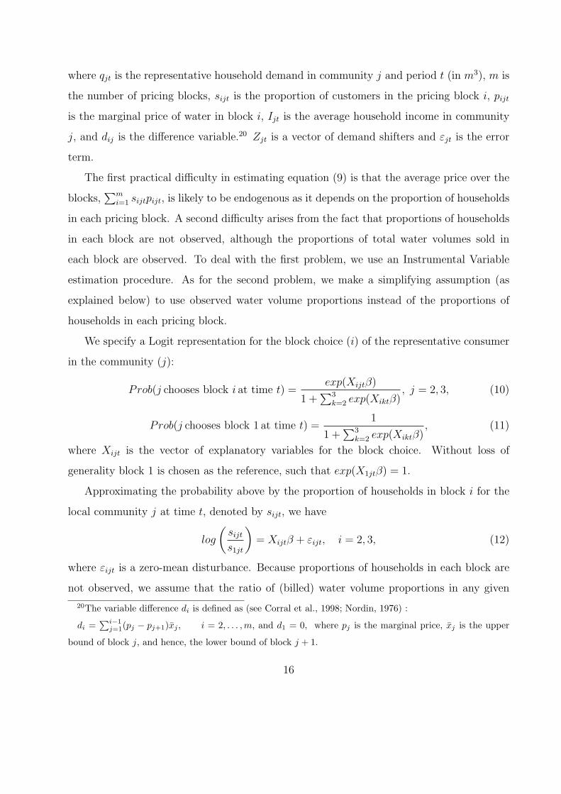
where qjt is the representative household demand in community j and period t (in m3), m is
the number of pricing blocks, sijt is the proportion of customers in the pricing block i, pijt
is the marginal price of water in block i, Ijt is the average household income in community
j, and dij is the difference variable.20 Zjt is a vector of demand shifters and εjt is the error
term.
The first practical difficulty in estimating equation (9) is that the average price over the
blocks,∑m
i=1 sijtpijt, is likely to be endogenous as it depends on the proportion of households
in each pricing block. A second difficulty arises from the fact that proportions of households
in each block are not observed, although the proportions of total water volumes sold in
each block are observed. To deal with the first problem, we use an Instrumental Variable
estimation procedure. As for the second problem, we make a simplifying assumption (as
explained below) to use observed water volume proportions instead of the proportions of
households in each pricing block.
We specify a Logit representation for the block choice (i) of the representative consumer
in the community (j):
Prob(j chooses block i at time t) =exp(Xijtβ)
1 +∑3
k=2 exp(Xiktβ), j = 2, 3, (10)
Prob(j chooses block 1 at time t) =1
1 +∑3
k=2 exp(Xiktβ), (11)
where Xijt is the vector of explanatory variables for the block choice. Without loss of
generality block 1 is chosen as the reference, such that exp(X1jtβ) = 1.
Approximating the probability above by the proportion of households in block i for the
local community j at time t, denoted by sijt, we have
log
(sijt
s1jt
)= Xijtβ + εijt, i = 2, 3, (12)
where εijt is a zero-mean disturbance. Because proportions of households in each block are
not observed, we assume that the ratio of (billed) water volume proportions in any given
20The variable difference di is defined as (see Corral et al., 1998; Nordin, 1976) :
di =∑i−1
j=1(pj − pj+1)xj , i = 2, . . . ,m, and d1 = 0, where pj is the marginal price, xj is the upper
bound of block j, and hence, the lower bound of block j + 1.
16
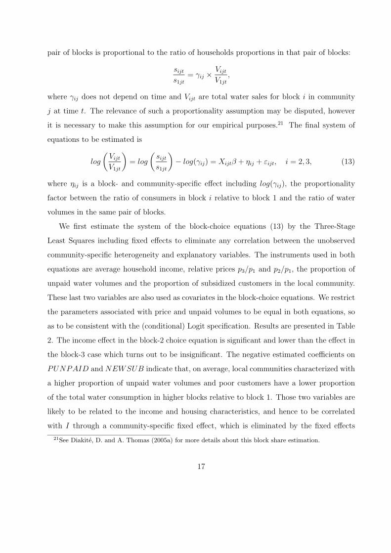
pair of blocks is proportional to the ratio of households proportions in that pair of blocks:
sijt
s1jt
= γij ×Vijt
V1jt
,
where γij does not depend on time and Vijt are total water sales for block i in community
j at time t. The relevance of such a proportionality assumption may be disputed, however
it is necessary to make this assumption for our empirical purposes.21 The final system of
equations to be estimated is
log
(Vijt
V1jt
)= log
(sijt
s1jt
)− log(γij) = Xijtβ + ηij + εijt, i = 2, 3, (13)
where ηij is a block- and community-specific effect including log(γij), the proportionality
factor between the ratio of consumers in block i relative to block 1 and the ratio of water
volumes in the same pair of blocks.
We first estimate the system of the block-choice equations (13) by the Three-Stage
Least Squares including fixed effects to eliminate any correlation between the unobserved
community-specific heterogeneity and explanatory variables. The instruments used in both
equations are average household income, relative prices p3/p1 and p2/p1, the proportion of
unpaid water volumes and the proportion of subsidized customers in the local community.
These last two variables are also used as covariates in the block-choice equations. We restrict
the parameters associated with price and unpaid volumes to be equal in both equations, so
as to be consistent with the (conditional) Logit specification. Results are presented in Table
2. The income effect in the block-2 choice equation is significant and lower than the effect in
the block-3 case which turns out to be insignificant. The negative estimated coefficients on
PUNPAID and NEWSUB indicate that, on average, local communities characterized with
a higher proportion of unpaid water volumes and poor customers have a lower proportion
of the total water consumption in higher blocks relative to block 1. Those two variables are
likely to be related to the income and housing characteristics, and hence to be correlated
with I through a community-specific fixed effect, which is eliminated by the fixed effects
21See Diakite, D. and A. Thomas (2005a) for more details about this block share estimation.
17
procedure. The price coefficient is highly significant and is of the expected sign, indicating
that the relative prices increase the probability of households being in the lower consumption
block.
[TABLE 2 ABOUT HERE]
The final estimation stage involves estimating structural demand parameters in Equation
(9) by fixed effects linear regression. The results are presented in Table 3, along with OLS
and GLS estimates.
[TABLE 3 ABOUT HERE]
From these estimates, price and income elasticities are easily computed, as well as their
standard errors with the Delta method. The price elasticity is equal to -0.8161 (with standard
error of 0.0853) and the income elasticity is 0.1462 (with standard error of 0.0367).
5 Simulation experiment
We now turn to our simulation experiment, that is, calibrating the optimal tariff designed
in section 3 with the parameter estimates obtained in section 4. As mentioned before, a
natural choice for the agent’s type is the households’ disposable income with the implicit
assumption that the demand for water is increasing in this variable. We first derive the
expression of the optimal nonlinear pricing rule when calibrated in the Cote d’Ivoire case.
The implementation of this optimal tariff is then simulated with various discretized versions
of the tariff, allowing the number of blocks and their bounds to vary.
5.1 Optimal nonlinear pricing
The system of nonlinear equations (5) to (8) is used to derive price pmin for the upper bound
qmin of the initial (social) pricing block, as well as the nonlinear pricing rule p(q) for water
volumes beyond qmin. The solution will depend on the parameters of elasticity of demand,
18
marginal production cost, statistical distribution of household, and the Ramsey number.
The elasticity parameters can be inferred from the estimation step, as follows: the elasticity
of demand with respect to the fixed fee, εQT , is directly related to the generalized demand
function in (3), and is equal to the income elasticity with the opposite sign. εQT is, therefore,
computed as β2×T/q). Also, we compute the price elasticity εQp by using demand estimates,
that is, εQp = β1 × P/q.
The marginal cost function c(q) is estimated from an additional data set obtained from
SODECI for the same local communities over the same period of time (Diakite and Thomas,
2005)22. The water supply cost is specified as a translog flexible form depending on out-
put level and input unit prices; and is estimated by imposing the usual homogeneity and
symmetry restrictions. The marginal cost is then a nonlinear function of output, which
is approximated by a linear regression to a polynomial of degree three: c(q) = 1141.17 −
11.58q + 0.0375q2 − 3.5× 10⁻⁶q3.
The density function of the household income is assumed to be Normal N(µ, σ2). After
rescaling the community-specific average household income (in FCFA) by a factor of 105, we
obtain µ = 25.87 and σ = 10.86.23
Finally, the Ramsey number is not identified and we arbitrarily set λ = 1, which gives
α = 0.5.24
The computation of welfare changes involves the master profile function defined in Equa-
tion (3). This profile can be defined as Q(P, p, q) = 1−prob[θ < θ(P, p, q)] = 1−F [θ(P, p, q))]
such that p = ∂U(q, θ)/∂q or, equivalently, q = q(p, θ), and with the condition that
U(q, θ) − P ≥ 0. Using the linear demand specification, the condition p(q, θ) ≥ p for
the agent with type θ is : θ = (q − β0 + β1p − δZ)/β2, with the inverse demand function
22An initial solution for the optimal tariff was obtained under the assumption of constant marginal cost,
however, this assumption was abandoned as it was rejected by the data.23We also experimented with an exponential distribution for the household income. The resulting optimal
price schedule was very similar in shape.24One feature of developing countries is the high opportunity cost of public funds. Many studies confirm
that this cost is higher there than in developed countries. It is typically estimated to lie between 1 and 3,
see Laffont (1996, 1999).
19
p(q, θ) = (β0 + β2θ − q + δZ)/β1.
The integral condition defining the master profile function has, in its general form, an
infinite upper bound. For the linear demand it is necessary to restrict the admissible values
of demand over the positive domain. This implies that q > 0 ⇔ p < p = (β0+β2θ+δZ)/β1.
Replacing the upper bound of the integral by p and integrating over the domain of p, we have
the conditions defining the generalized demand function as follows: θ ≥ (β1p+q−β0−δZ)/β2
and q2/2β1 − p . q − T ≥ 0.
The profile function is easily integrated numerically over the domain of q and/or p and
T , for computing any component of (consumer or producer) surplus.
The optimal tariff is finally obtained as follows. From Equation (7), we have that pmin =
Pmin/qmin. Replacing the elasticity εQT by its expression above, we obtain
Pmin = c(qmin).qmin +α
β2
qmin. (14)
so that
pmin = c(qmin) +α
β2
. (15)
We then solve for qmin in Equation (5), which reduces to
pmin − c(qmin) = α qmin
[f(θ)
β1
β2
], where θ =
β1pmin + qmin − β0 − δZ
β2
.
By replacing the marginal p by the solution for pmin, we obtain
1 = β1 qminf
[β1 [c(qmin) + α/β2] + qmin − β0 − δZ
β2
], (16)
where f is the density function of θ.
Substituting the solution for qmin in Equation (14), we obtain the value of the fixed fee,
Pmin. Finally, the nonlinear price p(q) can be computed from condition (8) as the solution
to
p(q) = c(q) + αβ1
β2
q f
[β1p(q) + q − β0 − δZ
β2
]. (17)
The nonlinear equation above is solved for p(q) using a numerical root-finding algorithm
over a grid of 100 points for consumption q ∈ [qmin, qmax]. The resulting nonlinear tariff is
20
presented in Figure 1. The optimal first (“social”) block is found to be between 0 and qmin
at 106 m3/year. Up to qmin, households pay a fixed charge Tmin (equal to Pmin) that is
Pmin = Tmin estimated at 66.24 USD /year.25
The monopoly pricing rule applies for volumes higher than 106 m3/year. On the decreas-
ing part of the tariff - up to 230 m3/year - this pricing rule starts with a minimum value
of p(qmin) at 0.67 USD /m3. The optimal marginal price is increasing between 230 and 500
m3/year, and beyond 500 m3/year, it is again decreasing. This non-monotonic pattern is
mainly due to the marginal cost estimate, which is approximated by a polynomial of order
3. For a typical household, water consumption is less than 200 m3 per year, and therefore it
would face a decreasing tariff.
[FIGURE 1 ABOUT HERE]
The optimal value for pmin is between 0.50 and 0.79 USD, the actual marginal prices for
the first and the second pricing block respectively. The total fixed fee in our experiment
is estimated at 16.56 USD, a value higher than the actual fixed payment of 4.02 USD/year
for the first block in the existing pricing rule. Further, the optimal social consumption
threshold in our case is substantially higher than the level observed in Cote d’Ivoire (106
m3/year versus 36 m3/year).
Although our simulated pair (pmin,qmin) departs from the existing one, however it em-
bodies some social considerations as, in the absence of the “social” constraint imposed on
the public decision-maker problem, the initial water volumes would have been charged at
marginal prices between 0.67 and 2.46 USD /m3. Moreover, qmin at 106 m3/year matches
the standard recommendations of the United Nations in terms of basic needs for a 6.5-person
household.
25or an equivalent marginal price of pmin = 66.24/106= 0.62 USD/m3.
21
5.2 Implementation : the multiblock tariff
To make the optimal tariff operational while preserving its main optimality features, we
consider a discrete version of the optimal nonlinear pricing rule in the form of a multi-block
tariff. The latter is designed to share the features of the optimal tariff, namely, universal
service obligations for low annual water consumption and an efficient monopoly pricing for
high annual water consumption. Note that in the optimal pricing design, we only need to
discretize the monopoly pricing expression as the initial block is already obtained above.
In making approximations to the optimal water tariffs, we consider two different trade-
offs that a public decision-maker may face. The first one is between simplicity of the tariff
and its optimality. It is well known from the empirical literature on water demand that
the effectiveness of price as a signal on the resource is better achieved through the tariffs
that are easily read by customers (monotonic price rates, limited number of pricing blocks).
The second trade-off is between optimality and equity of the water tariff. By modifying the
structure of the tariff, and possibly, departing from the optimal nonlinear one, it may be
possible to increase consumer welfare. To evaluate the impact on welfare of preferring the
tariff simplicity to its optimality, or equity to optimality, we compare four different water
tariffs.
Tariff 1. This is the existing one in Cote d’Ivoire, with an increasing block structure and
three block rates.
Tariff 2. Here we favor the tariff simplicity rather than its optimality, by designing tariff
blocks that are closest to the existing tariff, that has an increasing block rate structure.
Imposing a monotonic price schedule is very similar to the “ironing” procedure in Wilson
(1993) that consists in flattening the pricing rule so that the optimality condition is satisfied
on average. Tariff 2 only consists of three blocks, the first one being the “social” block
obtained from the nonlinear problem of Section 3. As detailed above, households pay only
a fixed fee P ∗min of 16.56 USD /quarter for consumption volumes up to q∗min at 106 m3/ year
which amounts to charging p1 equal to 0.62 USD / m3. The second block is designed to
impose a non-decreasing block rate structure, and it ranges from 106 m3 to 365 m3, the
22
volume for which the vertical line p2(= p(qmin)) at 0.67 USD / m3 cuts the optimal price
curve. Between 106 and 365 m3, the second block rate is simply p2(= p(qmin)) equal to
0.67 USD / m3. For the last block, beyond 365 m3 /year, we set the maximum unit rate
p3(= p(500)) at 0.77 USD / m3. Note that Tariff 2 is rather similar to Tariff 1 in terms of
the second block rate (0.77 USD /m3 versus 0.79 USD / m3), and in terms of the third block
upper bound (365 m3 /year in both cases).
Tariff 3. Contrary to Tariff 2, we favor optimality over the tariff simplicity, although
the number of block rates will be limited. More precisely, the non-decreasing condition is
relaxed, so as to correspond more closely to the optimal non linear pricing structure. The
first block of Tariff 3 is the predetermined social block for volumes below 106 m3/ year, as
under Tariff 2. As the optimal pricing rule is decreasing on the interval [106,230] m3, and
then increasing for volumes above 230 m3, we discretize the optimal tariff by considering
two blocks in the decreasing part and one block in the increasing part of the tariff. The
second block of Tariff 3 is from 106 to 190 m3 /year and the unit rate for this block is simply
determined by the monopoly pricing rule applied to the volume qmin of 106 m3 /year, that
is, p2(= p(qmin)) is 0.67 USD / m3. The third block corresponds to volumes between 190
and 230 m3/year, and its unit rate is computed as for block 2, that is, p3(= p(230)) is equal
to 0.10 USD / m3. The lower bound of the third block is determined arbitrarily, with the
objective to keep it sufficiently small due to the corresponding low value for the marginal
price. On the increasing part of the tariff, for volumes above 230 m3 / year, we consider
only one block and set the marginal price at its highest value possible, that is p4(= p(500))
is equal to 0.77 USD /m3.
Tariff 4. This tariff is an extension of Tariff 3. It is identical to Tariff 3 up to 230
m3/year, and has two additional pricing blocks in the high-volume region (i.e., we consider
three blocks instead of one). With this tariff, we are able to evaluate the impact on social
welfare of increasing the number of blocks in the water tariff, that is, when the degree of
discretization increases. Indeed, Wilson (1993) shows that when the number of blocks tends
to infinity, the multiple-block tariff converges to the optimal nonlinear pricing schedule p (q).
23
Hence, Tariff 4 allows one to evaluate the trade-off between optimality (better approximating
the optimal nonlinear tariff) and equity (the impact on welfare of increasing the number of
blocks).
[TABLE 4 ABOUT HERE]
Table 4 presents the block prices and bounds of the four tariffs. Except for the initial
consumption block, all unit rates in Tariff 1 (the existing tariff) are above the rates of our
proposed approximations to the optimal nonlinear pricing rule. This is particularly true for
consumption levels between 190 and 230 m3/year, where actual rates are almost twice the
value of Tariff 1 rates between 364 and 460 m3 (1.26 USD compared to 0.69 USD). Our
approximated multiblock tariffs always have unit price rates above the marginal cost, which
is in line with the Feldstein pricing rule discussed in Section 2.1. According to this policy,
setting unit rates systematically above marginal cost is a way to reduce the level of the fixed
charge. As mentioned in Section 2.3, Ivorian urban water utilities set a single fixed charge:
the connection fee, which is paid once and for all (and whose impact on the household
income is expected to be smoothed over a long period of time). Our approximation to the
optimal nonlinear pricing rule includes a fixed charge in the initial block (as long as there
is a strictly positive consumption level) which is higher than the existing one. Therefore,
the approximation to the optimal pricing rule tends to reduce inefficiency of the Feldstein
pricing rule, by pushing back unit rates in upper blocks toward the marginal cost, and by
increasing the fixed charge contained in the initial block.
5.3 Welfare comparisons
Our strategy here is to evaluate social welfare associated with the existing water tariff (Tariff
1), and to perform welfare comparisons with our proposed tariffs (Tariffs 2 to 4). We distin-
guish between the analysis for a representative household (irrespective of his/her income),
and a “poor” household (to be defined below).
24
Welfare computations for a representative household
We calculate the change in consumer welfare from the Marshallian consumer surplus for
a representative household in each local community (see the Appendix).26 Consumer surplus
variation (CSV ) is defined as the average amount each household would save every year if
the existing tariff (Tariff 1) is replaced by a proposed (simulated) tariff. Producer surplus
variation (PSV ) is the average annual loss per household the water operator would incur by
switching from Tariff 1 to a simulated tariff (Tariff 2, 3 or 4). Social welfare variation (WV )
is the average gain (or loss) per household for the society as a whole (represented here by the
representative consumer and the water operator). The welfare changes in relative terms are
obtained by dividing CSV and PSV by the average water expenditure of the representative
(average) household.
The welfare measures are computed for the country as a whole, using the sample-based
empirical distribution of income and proportions of water users in the different price blocks
for the full sample. If heterogeneity in operating conditions27 and in socio-demographic
characteristics of households throughout the country is likely to be significant, computing
such welfare variations at the regional level may be more interesting. To this end, we also
compute consumer and producer surpluses for each region, by using region-specific household
income distribution (mean and standard deviation for a Normal distribution) to calibrate
the optimal pricing rule.28
[TABLE 5 ABOUT HERE]
26While commonly adopted in applied welfare studies, the welfare change for a heterogeneous population
is not perfectly captured by the Marshallian consumer surplus, and an exact measure would require the
Hicksian demand curve. However, in the instance where only one price changes, Willig (1976) and Hausman
(1981) show that it is possible to compute consistent welfare changes using the Marshallian consumer surplus.27Even though SODECI is the major water operator in Cote d’Ivoire, each local community considered
here has its own production and distribution networks, and those communities are grouped into 10 Regional
Water Districts (DR, Directions Regionales).28Regions are the following: Southwest, Korhogo, Daloa, Bouak, Basse Cote, Abengourou, Yamoussoukro,
Man, Abidjan North, Abidjan South.
25
The results are presented in Table 5.29 Columns 3 to 5 of Table 5 report the relative
welfare changes associated with the switch from the existing tariff to Tariff 2, 3 and 4
respectively, for each of the 10 regions, and the entire country. They are in the same range
as those obtained in Garcia and Reynaud (2004) but contrast with those of Swallow and
Martin (1988) and Renzetti (1992).30
For the country as a whole (last row of Table 5), the change in social welfare from
switching to a proposed tariff is positive; however, there are significant differences across
regions. While most regions would gain from moving to Tariff 2, 3 or 4 (with a somewhat
limited gain for Abidjan North), Basse Cote and Abidjan-South regions would experience a
loss in social welfare. This result illustrates the need to account for heterogeneity in social
welfare variation at the regional level, when evaluating the implementation of the optimal
water pricing policies in countries like Cote d’Ivoire. The existing pricing policy is based
on a single (national) price system, which implies that there exist cross subsidies between
regions (in addition to the usual cross-subsidy mechanism between users in different block,
as implied by the block-rate price rule). Indeed, the city of Abidjan (North and South)
benefits from favorable hydrological conditions, and water production is relatively less costly
there (groundwater pumping, no filtration treatment). Moreover, the size and density of
the population (more than 4 million inhabitants and about 45,000 inhabitants per square
kilometer) allow to keep the water supply and customer service costs at a relatively lower
level than in other Ivorian cities. The city of Abidjan represents more than 50 percent of
all customers, about 60 percent of total billed volumes, 50 percent of expenditures and 60
percent of products (sales) in the water department of SODECI (Collignon, 2002). Therefore,
a homogeneous water tariff for the entire market of the SODECI concession seems to generate
a de facto subsidy, essentially financed by Abidjan residential customers for the benefit of
customers from other local communities in Cote d’Ivoire.
The evaluation of welfare changes associated with different price policies (say, Tariff k
29More detailed tables are omitted due to limited space, and are available from the authors upon request.30Garcia-Reynaud, Swallow-Martin and Renzetti found a 0.4, 2 and 4 percent increase in welfare respec-
tively.
26
vs. Tariff k′) is made possible by simply comparing welfare change from Tariff 1 to Tariff k
with the change generated by the move from Tariff 1 to Tariff k′. The optimality gain (or
equivalently, the loss in the tariff simplicity) generated by the move from Tariff 2 to Tariff
3 or 4 ultimately leads to a slight increase in the total welfare. Remember that Tariff 2 is
much closer to the existing one than Tariffs 3 and 4, which are not restricted to be of the
increasing-block type. The optimality gain generated by the move from Tariff 3 to Tariff
4 is associated with a decrease in total welfare, hence confirming the existence of a trade-
off between equity and efficiency. Moreover, surplus changes generated by these two tariffs
remain intimately related to the choice of pricing block bounds and corresponding marginal
prices.
Our results reveal that the existing pricing policy leads to a moderate social welfare gain
compared to approximations to the optimal tariff with the same number of blocks (Tariff
2). Based on our welfare computations, the optimal pricing policy would be to keep the
existing tariff (Tariff 1) for Abidjan (North and South) and Basse Cote regions, however, to
implement the approximated optimal Tariff 4 in all other regions of the country (because it
is closest to the optimal pricing rule). This is confirmed by the fact that in 2001 the budget
of a large majority of water services (except Abidjan) were actually in deficit.
Welfare analysis for a “poor” household
Since the objective of the water price policy is to increase water consumption by poorer
households while at the same time accounting for the operator benefit, it is necessary to
analyze the impact of our simulated tariffs on the welfare of these households. The individual
level analysis is not possible due to availability of only aggregate data, and we cannot adopt
a definition of poverty based on observed individual income. However, it seems reasonable
to assume that poor households that are connected to the water network will have their
consumption level in the first pricing block. We therefore define as “poor” a household
whose water consumption is below the upper bound of the social pricing block. By doing so,
the welfare comparison can be simply made by comparing the water bills a household would
27
pay when its consumption lies in the social pricing block, given the existing or alternative
tariffs. As our simulated Tariffs 2, 3 and 4 share the same first (“social”) block, we conduct
a simulation experiment at the regional level to compare the existing tariff (Tariff 1) with
any simulated tariff, on the basis of the social block only.
The region-specific empirical distribution of the household income is used to compute the
optimal first block for each region. The right-hand side of Table 5 reports the marginal price
pmin, the associated upper bound of the simulated social pricing block, qmin (in m3/year),
the welfare variation for the representative poor household (denoted by WLoss) and the
equivalent bill, BillEq. The latter corresponds to the bill a poor household would pay for a
volume corresponding to the (optimal) first block of the simulated tariff if it were charged
at the existing price.
We note a negative correlation between the average income µ and qmin, while pmin is
rather stable across regions. This relationship seems to indicate that the local communities
with a higher proportion of poor households (µ small) are those that require a higher volume
of water charged at the “social” rate corresponding to the first block.
At the national level, we obtain qmin equal to 106 m3/year with a marginal price pmin at
0.62 USD /m3. Under the existing water tariff, we have qmin at 76 m3/year and pmin at 0.50
USD/m3 respectively. Therefore, a household whose consumption is 106 m3 /year would
pay, according to the simulated tariff, a total water bill of Tmin equal to 66.24 USD/year.31
The same water consumption under the current tariff would cost the household BillEq of
61.65 USD / year.32 It seems that the poor household would pay slightly more with the
simulated tariff than with the existing one, with a welfare change of (BillEq−Tmin) at -4.59
USD a year.
This welfare loss for consumers from moving from Tariff 1 to any simulated tariff with an
optimal first block is, however, very limited when compared to the direct application of the
nonlinear pricing rule over the whole range of water volumes. Imposing the first block with
a flat rate is strongly in favor of poor households, who would pay much more for the first
31106 × 0.62 = 66.24.3218.10+(76-36)× 0.50+(106-76)× 0.79=61.65.
28
cubic meters if the nonlinear pricing rule were applied for those volumes. This is because
the optimal pricing rule is decreasing in the range of consumption that is concerned with
the social pricing policy. To impose the optimal tariff that has the “social” first block yields
a gain of about 90 USD a year to the representative consumer.
The fact that poor households benefit from the existing tariff as compared to the simu-
lated one suggests that introducing a charge-free consumption volume in the simulated tariffs
we consider may be an interesting option (see Gomez-Lobo and D. Contreras, 2000). The
“social” volume would simply be equivalent to the loss to households due to the new water
tariff. In our case, the representative poor household would be offered at least 8 m3/year33
so as to make the household indifferent between the actual and the simulated tariff. Al-
though the consumption of the household would be 106 m3/year, it would only be charged
98 m3/year.34
To compensate for the loss to the water service operator if water volumes are supplied
free of charge, several alternative tariff policies may be considered. More wealthy consumers
- whose consumption is above 190 m3/year in our experiment - may be excluded from the
benefit of the social pricing block. At their consumption level they would pay the simulated
optimal price between 0.67 and 2.46 USD /m3. The proposed tariff would then take the
form of a menu of tariffs according to the household type as follows:
Poor households (less than 106 m3/year ) Simulated tariffs
+ lump sum consumption depending on welfare loss
Medium-income households (between 106 and 190 m3/year)
Simulated tariffs
Well-off households (more than 190 m3/year ) Marginal price between 0.67 and 2.46 USD/m3 below 106 m3/year
Simulated tariffs above 106 m3/year.
In sum, the combination of the welfare analysis at the representative household level on
332067/292≈ 8.34106-8=98.
29
one hand, and at the poor household on the other, clearly reveals that the optimal tariff
policy, that includes social objectives as well as accounting for the operator profit, cannot be
achieved using a uniform price policy (for the whole concession market and all households).
Instead, along the lines of the region-specific tariffs, price schemes should incorporate a menu
of tariffs based on actual water consumption by the households.
6 Conclusion
This paper has tried to address the problem of the social water pricing in developing coun-
tries, where a general pricing policy is an increasing block tariff with a reduced-rate initial
block corresponding to basic needs. The main objective of the paper has been the design of
the optimal nonlinear tariff from the public regulator’s perspective where water is supplied
by a private operator facing heterogeneous consumers. Using Wilson’s (1993) definition of
the generalized demand profile, we propose an optimal pricing rule that combines both eq-
uity and efficiency considerations. The resulting tariff entails a fixed fee for the first block
of the tariff, presumably dedicated to low-income households, and a nonlinear pricing rule
for higher water volumes.
The optimal pricing rule is calibrated using econometric estimates of residential water
demand in Cote d’Ivoire, accounting for endogeneity of price as an explanatory variable,
and for the fact that the existing tariff has several price rates. Several approximations to
the optimal tariff are computed in the form of multiblock tariffs. The impact on welfare of
favoring the tariff simplicity to imposing an increasing block rate structure is then evaluated.
The results are compared to the existing, increasing-block tariff water pricing in Cote d’Ivoire,
and welfare change calculations are performed.
Our results enable us to draw two conclusions. First, the homogeneous water price
system over the entire market of the concession is not optimal and can be improved by using
essentially the same tariff structure as the existing one. However, total welfare changes are
not expected to be large, as producer losses almost compensate for gains in the consumer
30

welfare. Second, a better pricing system can be obtained by keeping the existing tariffs in
Abidjan and Basse Cote35 and adopting our proposed tariffs in the other regions. Moreover,
the welfare analysis conducted for poor households reveals the need for classifying households
in different categories within the same community, as well as proposing a menu of tariffs.
Such a menu - derived from our simulated optimal tariffs - would then allow to improve the
trade off between social objectives on one hand, and the operator financial outlook on the
other.
35a region very close to Abidjan
31
References
[1] Baumol, W.J. (1987). Ramsey pricing. In The New Palgrave, J. Eatwell, M. Milgate
and P. Newman (eds.), vol IV, 49-51. Macmillan Press Ltd., London.
[2] Boland, J.J. and D. Whittington (2000). The political economy of water tariff design
in developing countries: Increasing block tariffs versus uniform price with rebate. In
The political economy of water pricing reforms, Ariel Dinar (ed.), pp. 215-235. Oxford
University Press, Oxford.
[3] Brown S. and D. Sibley (1986). The Theory of Public Utility Pricing, Cambridge Uni-
versity Press.
[4] Burtless, G. and J. Hausman, (1978). The Effect of Taxation on Labor Supply: Eval-
uating the Gary Negative Income Tax Experiment. Journal of Political Economy 86,
1103-1130.
[5] Chicoine, D., S. Deller, and G. Ramamurthy (1986). Water Demand Estimation Under
Block Rate Pricing : A Simultaneous Equation Approach. Water Resources Research
22, 859-863.
[6] Collignon, B. (2002). Urban Water Supply Innovations in Cote d’lvoire: How Cross-
Subsidies Help the Poor. Nairobi: Water and Sanitation Program - Africa, 2002.
[7] Collignon, B., R. Taisne, and J.-M. S. Kouadio (2000). Water and Sanitation for the
Urban Poor in Cote d’Ivoire. Nairobi: Water and Sanitation Program - Africa, 2002.
[8] Corral, L., A. Fischer, and N. Hatch (1998). Price and Non-Price Influences on Water
Conservation: An Econometric Model of Aggregate Demand under Non Linear Budget
Constraint. Working Paper No 881, Department of Agricultural and Resource Eco-
nomics and Policy, University of California at Berkeley.
32
[9] Diakite, D. and A. Thomas (2005). Structure des Couts d’Alimentation en Eau Potable
: Une Application aux Donnees des Centres de Production Ivoiriens. Gremaq Working
Paper, University of Toulouse.
[10] Diakite, D. and A. Thomas (2006). La Demande d’Eau a Usage Residentiel en Cote
d’Ivoire : Une Analyse Econometrique sur Donnees de Panel. Gremaq Working Paper,
University of Toulouse.
[11] Garcia, S. and A. Reynaud (2004). Estimating the benefits of Efficient Water Pricing
in France. Resource and Energy Economics 26, 1-25.
[12] Gleick, P.H. (1996). Basic water requirements for human activities: Meeting human
needs. Water International 21, 83-92.
[13] Gomez-Lobo, A. and D. Contreras (2000). Water subsidy policies: A comparison of the
Chilean and Colombian schemes. The World Bank Economic Review 17, 391-407.
[14] Hausman, J.A. (1981). Exact Consumer’s Surplus and Deadweight Loss. American Eco-
nomic Review 71, 662-676.
[15] Hewitt, J. and W. Hanemann (1995). A Discrete/continuous Choice Approach to Resi-
dential Water Demand under Block Rate Pricing. Land Economics 71, 173-192.
[16] Laffont, J.J.(1999). Competition Information and Development. Annual World Bank
Conference on Development Economics 1998, The World Bank, Washington D.C.
[17] Laffont, J.J.( 1996). Regulation, Privatisation and Incentives in Developing Countries.
Current Issues in Economic Development, Oxford University Press, Oxford.
[18] Laffont, J.J. and J. Tirole (2000). Competition on telecommunications. MIT Press,
Cambridge, MA.
[19] Laffont, J.-J. and J. Tirole (1993). A Theory of Incentives in Procurement and Regula-
tion. MIT Press, Cambridge.
33
[20] Martinez-Espineira, R., (2003). Estimating Water Demand under Increasing Block Tar-
iffs Using Aggregate Data and Proportions of Users per Block. Environmental and Re-
source Economics 26, 5-23.
[21] Menard, C., and G. Clarke (2000). Reforming the Water Supply in Abidjan, Cote
d’Ivoire : Mild Reform in a Turbulent Environment. Working paper Series 2377, The
World Bank, Washington, D.C.
[22] Moffitt, R. (1986). The Econometrics of Piecewise-linear Budget Constraints. Journal
of Business and Economic Statistics 4, 317-328.
[23] Moffitt, R. (1990). The Econometrics of Kinked Budget Constraints. Journal of Eco-
nomic Perspectives 4, 119-139.
[24] Nordin, J. (1976). A Proposed Modification on Taylor’s Demand-Supply Analysis: Com-
ment. Bell Journal of Economic Management and Science 7, 719-721.
[25] Prieger, J.E. (1996). Ramsey pricing and competition: the consequences of myopic
regulation. Journal of Regulatory Economics 10, 307-321.
[26] Renzetti, S. and J. Kushner (2004). Full cost accounting for water supply and sewage
treatment: Concepts and case application. Canadian Water Resources Journal 29, 13-
22.
[27] Renzetti, S. (2000). An empirical perspective on water pricing reforms. In The political
economy of water pricing reforms, Ariel Dinar (ed.), pp. 123-140. Oxford University
Press, Oxford.
[28] Renzetti, S. (1992). Evaluating the Welfare Effects of Reforming Municipal Water
Prices. Journal of Environment Economics and Management 22, 147-192.
[29] Shefter, J., and E. David (1985). Estimating Residential Water Demand Under Multi-
part Tariffs Using Aggregate Data. Land Economics 61, 21-33.
34
[30] Strand, J., and I. Walker (2005). Water markets and demand in Central America. En-
vironment and Development Economics 10, 313-335.
[31] Swallow, S. and C. Martin (1988). Long Run Price Inflexibility and Efficiency Loss for
Municipal Water Supply. Journal of Environmental Economics and Management 15,
233-247.
[32] Willig, R. (1976). Consumer Surplus without Apology. American Economic Review 66,
589-597.
[33] Wilson, R. (1993). Nonlinear Pricing. Oxford University Press, Oxford.
35
7 Appendix
Welfare computations
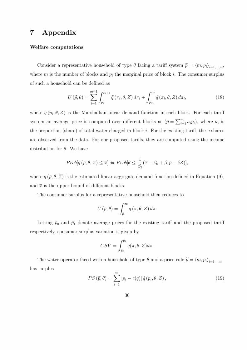
Consider a representative household of type θ facing a tariff system p = 〈m, pi〉i=1,...,m,
where m is the number of blocks and pi the marginal price of block i. The consumer surplus
of such a household can be defined as
U (p, θ) =m−1∑i=1
∫ pi+1
pi
q (πi, θ, Z) dπi +
∫ ∞
pm
q (πi, θ, Z) dπi, (18)
where q (pi, θ, Z) is the Marshallian linear demand function in each block. For each tariff
system an average price is computed over different blocks as (p =∑m
i=1 aipi), where ai is
the proportion (share) of total water charged in block i. For the existing tariff, these shares
are observed from the data. For our proposed tariffs, they are computed using the income
distribution for θ. We have
Prob[q (p, θ, Z) ≤ x] ⇔ Prob[θ ≤ 1
β2
(x− β0 + β1p− δZ)],
where q (p, θ, Z) is the estimated linear aggregate demand function defined in Equation (9),
and x is the upper bound of different blocks.
The consumer surplus for a representative household then reduces to
U (p, θ) =
∫ ∞
p
q (π, θ, Z) dπ.
Letting p0 and p1 denote average prices for the existing tariff and the proposed tariff
respectively, consumer surplus variation is given by
CSV =
∫ p1
p0
q(π, θ, Z)dπ.
The water operator faced with a household of type θ and a price rule p = 〈m, pi〉i=1,...,m
has surplus
PS (p, θ) =m∑
i=1
[pi − c(q)] q (pi, θ, Z) , (19)
36
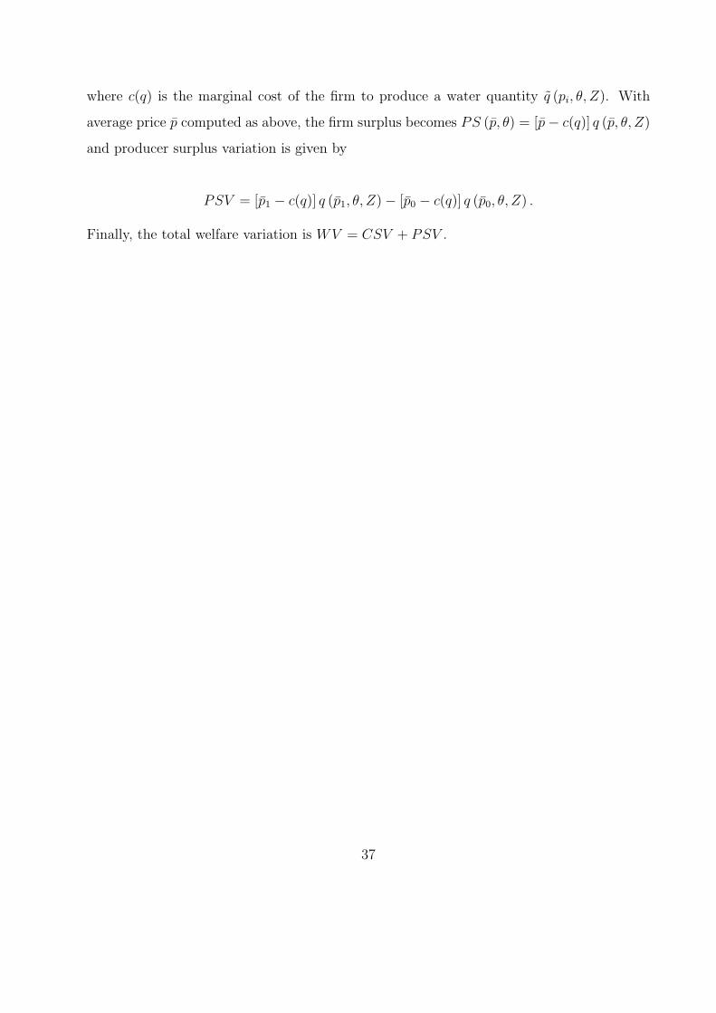
where c(q) is the marginal cost of the firm to produce a water quantity q (pi, θ, Z). With
average price p computed as above, the firm surplus becomes PS (p, θ) = [p− c(q)] q (p, θ, Z)
and producer surplus variation is given by
PSV = [p1 − c(q)] q (p1, θ, Z)− [p0 − c(q)] q (p0, θ, Z) .
Finally, the total welfare variation is WV = CSV + PSV .
37
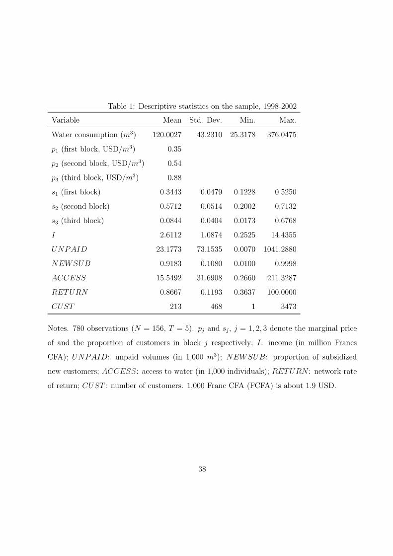
Table 1: Descriptive statistics on the sample, 1998-2002
Variable Mean Std. Dev. Min. Max.
Water consumption (m3) 120.0027 43.2310 25.3178 376.0475
p1 (first block, USD/m3) 0.35
p2 (second block, USD/m3) 0.54
p3 (third block, USD/m3) 0.88
s1 (first block) 0.3443 0.0479 0.1228 0.5250
s2 (second block) 0.5712 0.0514 0.2002 0.7132
s3 (third block) 0.0844 0.0404 0.0173 0.6768
I 2.6112 1.0874 0.2525 14.4355
UNPAID 23.1773 73.1535 0.0070 1041.2880
NEWSUB 0.9183 0.1080 0.0100 0.9998
ACCESS 15.5492 31.6908 0.2660 211.3287
RETURN 0.8667 0.1193 0.3637 100.0000
CUST 213 468 1 3473
Notes. 780 observations (N = 156, T = 5). pj and sj, j = 1, 2, 3 denote the marginal price
of and the proportion of customers in block j respectively; I: income (in million Francs
CFA); UNPAID: unpaid volumes (in 1,000 m3); NEWSUB: proportion of subsidized
new customers; ACCESS: access to water (in 1,000 individuals); RETURN : network rate
of return; CUST : number of customers. 1,000 Franc CFA (FCFA) is about 1.9 USD.
38
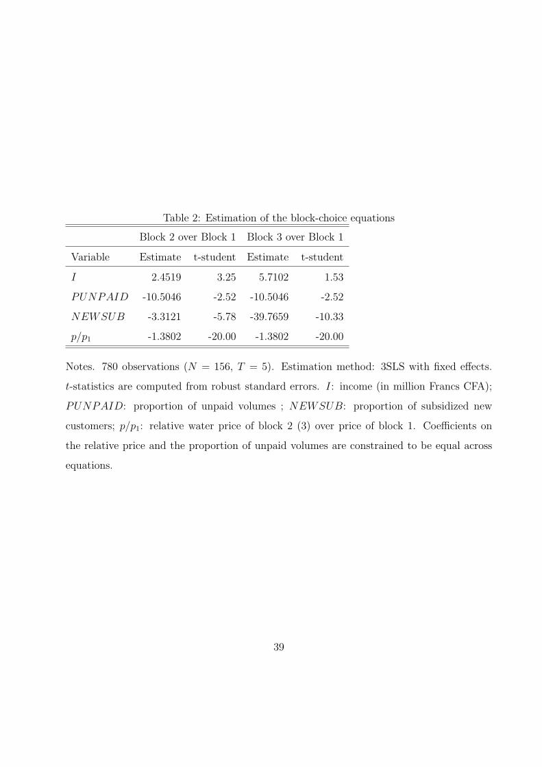
Table 2: Estimation of the block-choice equations
Block 2 over Block 1 Block 3 over Block 1
Variable Estimate t-student Estimate t-student
I 2.4519 3.25 5.7102 1.53
PUNPAID -10.5046 -2.52 -10.5046 -2.52
NEWSUB -3.3121 -5.78 -39.7659 -10.33
p/p1 -1.3802 -20.00 -1.3802 -20.00
Notes. 780 observations (N = 156, T = 5). Estimation method: 3SLS with fixed effects.
t-statistics are computed from robust standard errors. I: income (in million Francs CFA);
PUNPAID: proportion of unpaid volumes ; NEWSUB: proportion of subsidized new
customers; p/p1: relative water price of block 2 (3) over price of block 1. Coefficients on
the relative price and the proportion of unpaid volumes are constrained to be equal across
equations.
39
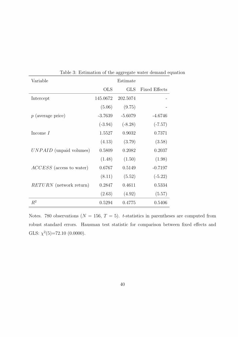
Table 3: Estimation of the aggregate water demand equation
Variable Estimate
OLS GLS Fixed Effects
Intercept 145.0672 202.5074 -
(5.06) (9.75) -
p (average price) -3.7639 -5.6079 -4.6746
(-3.94) (-8.28) (-7.57)
Income I 1.5527 0.9032 0.7371
(4.13) (3.79) (3.58)
UNPAID (unpaid volumes) 0.5809 0.2082 0.2037
(1.48) (1.50) (1.98)
ACCESS (access to water) 0.6767 0.5149 -0.7197
(8.11) (5.52) (-5.22)
RETURN (network return) 0.2847 0.4611 0.5334
(2.63) (4.92) (5.57)
R2 0.5294 0.4775 0.5406
Notes. 780 observations (N = 156, T = 5). t-statistics in parentheses are computed from
robust standard errors. Hausman test statistic for comparison between fixed effects and
GLS: χ2(5)=72.10 (0.0000).
40
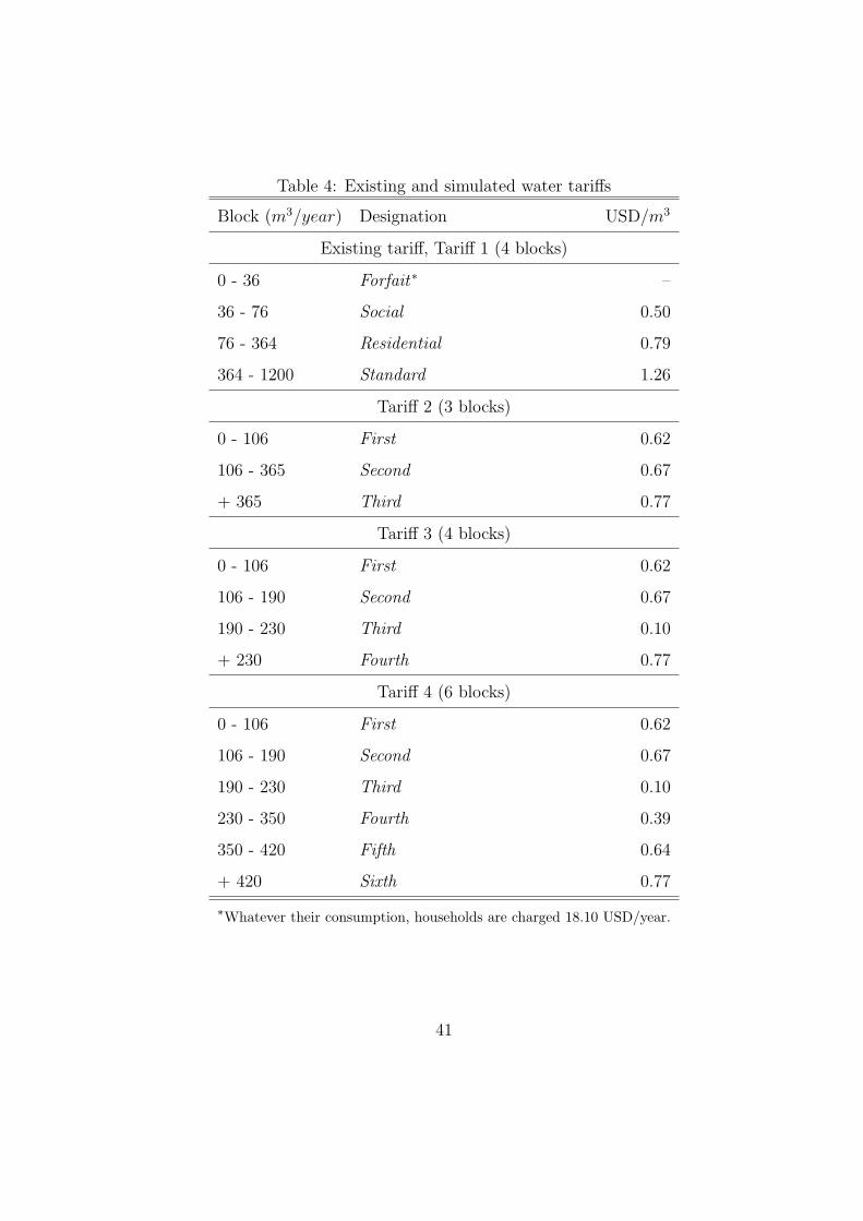
Table 4: Existing and simulated water tariffs
Block (m3/year) Designation USD/m3
Existing tariff, Tariff 1 (4 blocks)
0 - 36 Forfait∗ –
36 - 76 Social 0.50
76 - 364 Residential 0.79
364 - 1200 Standard 1.26
Tariff 2 (3 blocks)
0 - 106 First 0.62
106 - 365 Second 0.67
+ 365 Third 0.77
Tariff 3 (4 blocks)
0 - 106 First 0.62
106 - 190 Second 0.67
190 - 230 Third 0.10
+ 230 Fourth 0.77
Tariff 4 (6 blocks)
0 - 106 First 0.62
106 - 190 Second 0.67
190 - 230 Third 0.10
230 - 350 Fourth 0.39
350 - 420 Fifth 0.64
+ 420 Sixth 0.77
∗Whatever their consumption, households are charged 18.10 USD/year.
41
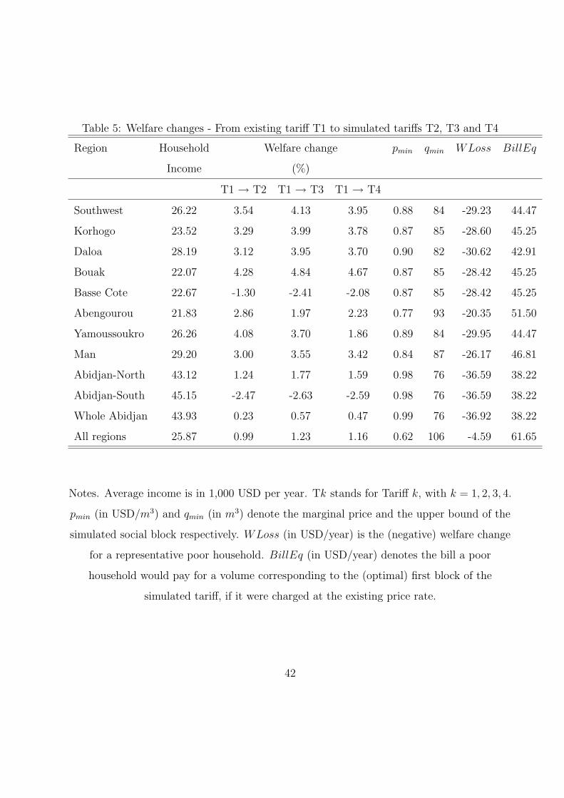
Table 5: Welfare changes - From existing tariff T1 to simulated tariffs T2, T3 and T4
Region Household Welfare change pmin qmin WLoss BillEq
Income (%)
T1 → T2 T1 → T3 T1 → T4
Southwest 26.22 3.54 4.13 3.95 0.88 84 -29.23 44.47
Korhogo 23.52 3.29 3.99 3.78 0.87 85 -28.60 45.25
Daloa 28.19 3.12 3.95 3.70 0.90 82 -30.62 42.91
Bouak 22.07 4.28 4.84 4.67 0.87 85 -28.42 45.25
Basse Cote 22.67 -1.30 -2.41 -2.08 0.87 85 -28.42 45.25
Abengourou 21.83 2.86 1.97 2.23 0.77 93 -20.35 51.50
Yamoussoukro 26.26 4.08 3.70 1.86 0.89 84 -29.95 44.47
Man 29.20 3.00 3.55 3.42 0.84 87 -26.17 46.81
Abidjan-North 43.12 1.24 1.77 1.59 0.98 76 -36.59 38.22
Abidjan-South 45.15 -2.47 -2.63 -2.59 0.98 76 -36.59 38.22
Whole Abidjan 43.93 0.23 0.57 0.47 0.99 76 -36.92 38.22
All regions 25.87 0.99 1.23 1.16 0.62 106 -4.59 61.65
Notes. Average income is in 1,000 USD per year. Tk stands for Tariff k, with k = 1, 2, 3, 4.
pmin (in USD/m3) and qmin (in m3) denote the marginal price and the upper bound of the
simulated social block respectively. WLoss (in USD/year) is the (negative) welfare change
for a representative poor household. BillEq (in USD/year) denotes the bill a poor
household would pay for a volume corresponding to the (optimal) first block of the
simulated tariff, if it were charged at the existing price rate.
42