Embed Size (px)
Citation preview

A Problem-Solving Methodology Based on ExtremalityPrinciple and its Application to CS Education
Submitted in partial fulfillment of
the requirements of the degree of
Doctor of Philosophy
by
Jagadish M.
(Roll No. 09405007)
Under the guidance of
Prof. Sridhar Iyer
DEPARTMENT OF COMPUTER SCIENCE & ENGINEERING
INDIAN INSTITUTE OF TECHNOLOGY – BOMBAY
2015


Abstract
Extremality principle is a commonly used problem-solving strategy. The main idea is to
look at extremal cases of a problem in order to obtain insight about the general structure.
Though the principle is widely known, it is not explicitly discussed in algorithm textbooks
or taught in courses. We devise a methodology based on extremality principle and use it
to solve a variety of algorithmic problems involving graphs. We apply the methodology to
three tasks that are relevant in the context of teaching algorithms.
The first task is related to the analysis of greedy algorithms. We are given an optimiza-
tion problem P and a greedy algorithm that is purported to solve the problem P. The goal is
to construct an instance of P on which the algorithm fails to give the correct answer. Such
an instance is called a counterexample. In a pilot experiment, we found that students had
difficulty in constructing counterexamples. We give a method to construct counterexamples
for many graph-theoretic problems. We apply our method to standard problems in graph
theory for which greedy algorithms exist in literature.
The second task is related to proving lower bounds on a query computational model.
We are given a graph G as input via its adjacency matrix A. We are also given a graph
property (like connectivity). The goal is to determine the minimum number of entries of A
that one needs to probe in order to check if G has the given property. We prove that if the
graph has n nodes, then for many common properties at least Ω(n2) probes are necessary.
We find that lower bound proofs of this problem that are given in textbooks rely too much
on ‘connectivity’ property and do not generalize well. We give a method to prove lower
bounds in a systematic way. In a pilot experiment, we found that students were able to
understand and apply our method.
In the third task we use our methodology to solve a research problem. We give a
detailed account of the problem-solving process that could be of expository value.
We present preliminary work to show the use of extremality in linear programming.
i

ii

Contents
Abstract v
1 Introduction 1
1.1 Mathematical Problem-Solving . . . . . . . . . . . . . . . . . . . . . . . . . . . . . 1
1.2 Extremality Principle . . . . . . . . . . . . . . . . . . . . . . . . . . . . . . . . . . . 3
1.3 Main Contributions . . . . . . . . . . . . . . . . . . . . . . . . . . . . . . . . . . . . 4
1.4 Thesis Organization . . . . . . . . . . . . . . . . . . . . . . . . . . . . . . . . . . . . 5
2 WISE Methodology 7
2.1 WISE: Weaken-Identify-Solve-Extend . . . . . . . . . . . . . . . . . . . . . . . . . 7
2.2 Example I: Intersecting Intervals . . . . . . . . . . . . . . . . . . . . . . . . . . . . 12
2.3 Example II: Harmonic Vertices . . . . . . . . . . . . . . . . . . . . . . . . . . . . . 13
2.4 Example III: Coins in a Row . . . . . . . . . . . . . . . . . . . . . . . . . . . . . . . 15
2.5 Example IV: Grid Minimum . . . . . . . . . . . . . . . . . . . . . . . . . . . . . . . 17
2.6 Discussion . . . . . . . . . . . . . . . . . . . . . . . . . . . . . . . . . . . . . . . . . 21
3 Constructing Counterexamples using WISE 23
3.1 Introduction . . . . . . . . . . . . . . . . . . . . . . . . . . . . . . . . . . . . . . . . 23
3.2 Definitions . . . . . . . . . . . . . . . . . . . . . . . . . . . . . . . . . . . . . . . . . 24
3.3 Anchor Method . . . . . . . . . . . . . . . . . . . . . . . . . . . . . . . . . . . . . . 27
3.4 Anchor Method using MIS as an Illustrative Example. . . . . . . . . . . . . . . . 27
3.5 Role of Extremality . . . . . . . . . . . . . . . . . . . . . . . . . . . . . . . . . . . . 31
3.6 Additional Examples . . . . . . . . . . . . . . . . . . . . . . . . . . . . . . . . . . . 34
3.7 Pilot Experiment . . . . . . . . . . . . . . . . . . . . . . . . . . . . . . . . . . . . . . 50
3.8 Discussion . . . . . . . . . . . . . . . . . . . . . . . . . . . . . . . . . . . . . . . . . 54
iii

4 Proving Query Lower Bounds using WISE 55
4.1 Introduction . . . . . . . . . . . . . . . . . . . . . . . . . . . . . . . . . . . . . . . . 55
4.2 Query Complexity . . . . . . . . . . . . . . . . . . . . . . . . . . . . . . . . . . . . . 56
4.3 Related Work . . . . . . . . . . . . . . . . . . . . . . . . . . . . . . . . . . . . . . . . 58
4.4 Adversary Argument Revisited . . . . . . . . . . . . . . . . . . . . . . . . . . . . . 59
4.5 Scope of Problems . . . . . . . . . . . . . . . . . . . . . . . . . . . . . . . . . . . . . 61
4.6 Query lower bounds using WISE . . . . . . . . . . . . . . . . . . . . . . . . . . . . 62
4.7 Main Theorem . . . . . . . . . . . . . . . . . . . . . . . . . . . . . . . . . . . . . . . 63
4.8 Applications . . . . . . . . . . . . . . . . . . . . . . . . . . . . . . . . . . . . . . . . 64
4.9 Teachability . . . . . . . . . . . . . . . . . . . . . . . . . . . . . . . . . . . . . . . . . 69
4.10 Discussion . . . . . . . . . . . . . . . . . . . . . . . . . . . . . . . . . . . . . . . . . 72
5 Tree Learning Algorithm using WISE 73
5.1 Iteration 1: From path to bounded leaves tree . . . . . . . . . . . . . . . . . . . 75
5.2 Iteration 2: From binary tree to short diameter . . . . . . . . . . . . . . . . . . . 77
5.3 Iteration 3: From centipede to long diameter tree . . . . . . . . . . . . . . . . . 80
5.4 A Sub-Quadratic Algorithm . . . . . . . . . . . . . . . . . . . . . . . . . . . . . . . 87
5.5 Discussion . . . . . . . . . . . . . . . . . . . . . . . . . . . . . . . . . . . . . . . . . 88
6 Extremality in Linear Programming 89
6.1 Motivation . . . . . . . . . . . . . . . . . . . . . . . . . . . . . . . . . . . . . . . . . 89
6.2 Preliminaries . . . . . . . . . . . . . . . . . . . . . . . . . . . . . . . . . . . . . . . . 90
6.3 Problems . . . . . . . . . . . . . . . . . . . . . . . . . . . . . . . . . . . . . . . . . . 92
6.4 Discussion . . . . . . . . . . . . . . . . . . . . . . . . . . . . . . . . . . . . . . . . . 105
7 Conclusion 107
7.1 Direct proofs vs WISE . . . . . . . . . . . . . . . . . . . . . . . . . . . . . . . . . . 107
7.2 Problems related to teachability of WISE . . . . . . . . . . . . . . . . . . . . . . . 108
iv

Chapter 1
Introduction
1.1 Mathematical Problem-Solving
Problem-solving research has a long history. We give an overview of findings of the mathe-
matics community that are relevant to our work. Although teachers having been interested
in problem-solving for over a century it was Polya’s book ‘How to solve it’ that gave impetus
to research in the subject. The book contains a variety of heuristics that are commonly
used by mathematicians. Early research on the topic described thinking processes used by
individuals as they solved problems. Experiments suggested that the key factors that in-
fluenced problem-solving were knowledge, meta-cognitive skills and beliefs. In the 1970s
and 80s, researchers like Schoenfeld and Lester observed the outcomes of teaching Polya-
style heuristics directly to students in classrooms. A consensus among researchers that has
emerged is that while meta-cognitive skills play an important role in problem-solving there
is little evidence to show that these skills can be taught to students. Schoenfeld’s work
shows that teaching general heuristics to students does not improve their problem-solving
ability ([30], [31]). A nice summary of problem-solving research can be found in the book
‘Theories of Mathematics Education’ by Bharath Sriraman and Lyn English [32]. To quote
from the book:
Teaching students about problem-solving strategies and heuristics and phases of
problem solving does little to improve students’ ability to solve general math-
ematics problems ([22] p. 508). For many mathematics educators, such a
consistent finding is disconcerting.
1

The ineffectiveness of heuristics is commonly attributed to two main drawbacks:
Drawback 1. Scope of problems is too broad. The scope of problems solvable by a heuris-
tic is usually ill-defined; this makes it difficult to judge when a particular heuristic is
applicable. Choosing the right procedure from a long list itself can become daunting.
(pg. 265 [32]). Polya’s book alone has about forty heuristics.
Drawback 2. Lack of predictive power. Even if one finds the correct heuristic for a given
problem, its descriptive nature makes it hard to directly apply it to the problem. Most
heuristics are often just names given for broad thinking processes. The same heuris-
tic like ‘solve an analogical problem’ can be interpreted in many ways and applies
differently to different problems [30].
Techniques such as greedy, divide-and-conquer, dynamic programming are based on
some popular heuristics in mathematical problem-solving. For example, divide-and-conquer
is based on the following heuristic: ‘Decompose the problem and recombine its elements in
some new manner’ (pg. 75 [27]). We show how the divide-and-conquer technique differs
from the heuristic by arguing that it addresses the drawbacks mentioned above.
Scope of problems. There is empirical evidence to show that divide-and-conquer strategy
is useful usually when one encounters the following situation: An easy polynomial
algorithm can be found but one suspects that an improvement is possible. The strat-
egy rarely improves the running time by more than an O(n) factor. For example, all
the problems (including exercises) mentioned in popular textbooks like [6], [7] and
[21] belong to this category. Table 1.1 shows some common examples.
Predictive Power. The chapter on divide-and-conquer is a collection of illustrative exam-
ples and technical tools for solving recurrences [6]. The examples and the exercises
given the chapter are representative of the problems that one encounters in computer
science. It is plausible that ideas used in solving the textbook problems also help in
solving other (unseen) problems. Divide-and-conquer based solutions usually involve
recurrences. Hence, a few technical tools have been developed to solve recurrences of
various kinds [9]. The ability to solve recurrences can be seen as one of the core-skills
of using divide-and-conquer technique. Hence, it it not surprising that four out of the
six sections in the chapter from CLRS textbook deal with solving recurrences (Chap.
2

Problem Naïve Divide and Conquer
Sorting O(n2) O(n log n)
Counting Inversions O(n2) O(n log n)
Matrix Multiplication O(n3) O(n2.7)
Maximum Subarray O(n2) O(n log n)
Closest Pair of Points O(n2) O(n log n)
Hidden Surface Removal O(n2) O(n log n)
Integer Multiplication O(n2) O(n log n)
Convolution and FFT O(n2) O(n log n).
Table 1.1: Problems discussed in the chapter on divide-and-conquer in popular textbooks like CLRS
[6] and Klienberg-Tardos [21]. For each problem, the table shows the running time of the naïve
algorithm and the divide-and-conquer algorithm. Divide-and-conquer strategy usually gives only a
o(n) factor improvement over the naïve algorithm.
4 [6]). It is the illustrative examples and the technical tools for solving recurrences
together as a ‘package’ that gives the divide-and-conquer technique some predictive
power.
We propose a methodology that operationalizes Polya’s heuristic of solving easier
problems first. The process of finding easier problems is referred to as ‘Weaken-
ing’. We extend the solution of the easier problem to solve the original problem.
We call our methodology as ‘WISE’. WISE stands for ‘Weaken-Identify-Solve-Extend’
(Fig. 1.1).
1.2 Extremality Principle
The extremality principle is a problem-solving strategy that involves studying objects with
extreme properties in order to reason about more general objects. Although the principle
is intuitive and well-known, its application to a specific problem can be difficult. There are
many books on problem-solving that illustrate the use of extremality principle in solving
3

Heuristic. “Can you decompose the
problem and recombine its elements in
some new manner?”
⇓Operationalize
Divide and Conquer
Core Skill: Solving Recurrences.
Heuristic. “If you can’t solve a prob-
lem, then there is an easier problem
you can solve: find it.”
⇓Operationalize
WISE
Core Skill: Finding Extremal Instances.
Figure 1.1: Analogy between divide-and-conquer and WISE.
mathematical problems ([8], [27]). However, the current texts on extremality principle
focus mostly on math topics like geometry, number theory and combinatorics.
In computer science, extremality is discussed only in the context of greedy algorithms.
A greedy algorithm makes a local choice at each step that is extremal in some sense. Con-
struction of extremal graphs is also an important topic in graph theory. Extremal graphs
are those which maximize or minimize certain functions on properties. For example, some
simple extremal graphs are shown in Table 1.2. A complete graph is extremal since it max-
imizes the number of edges. A path is extremal since it has the longest diameter, and so
on.
We use the extremality principle to give more predictive power to the methodology.
In all the applications that we solve, we will show how extremal graphs play a key role in
solving the problems. The ideas in our technique are well-known to experts who probably
apply them implicitly. We make the use of extremal graphs explicit.
1.3 Main Contributions
The main contributions of the thesis are as follows:
• A method to construct counterexamples for greedy algorithms for optimization prob-
lems in graph theory.
• A method to prove lower bounds for graph property-testing under the query-complexity
model.
4

Common Extremal Graphs
Path
Cycle
Star
Complete graphKn
Independent set graphIn
Binary Tree
Complete bipartite graph
Kn,n
Table 1.2: Generic extremal graphs which play an important role is solving many graph-theoretic
problems.
• An O(n1.8 log n) algorithm for the tree learning problem and its derivation using the
WISE methodology.
• A list of instructive examples for linear programming using the extremality principle.
1.4 Thesis Organization
• In chapter 2, we describe the WISE methodology apply it to solve a few textbook
problems. The problems are chosen from undergraduate algorithms textbooks.
• In chapter 3, we show how the WISE methodology can be used to construct coun-
terexamples for greedy algorithms. We show the applicability of the technique for
many standard problems in graph theory for which greedy algorithms exist in litera-
ture.
• In chapter 4, we apply WISE to problems related to property-testing in graph theory
under the query-complexity model.
• In chapter 5, we use WISE to derive an algorithm for a problem called the ‘tree
5

learning problem’. The objective is to find the structure of a bounded-degree tree
using minimum number of queries to a separator oracle. The separator oracle can
answer queries of the form “Does the node x lie on the path from node a to node b?”.
We derive an O(n1.8 log n) algorithm using WISE for this problem which improves
upon the previously known quadratic bound.
• In chapter 6, we discuss the potential use of extremality principle in the topic of linear
programming.
• In chapter 7, we give some possible extensions of the methods discussed in the previ-
ous chapters.
WISE
Chap. 2: Illustrations Applications of WISE
Chap. 3: Counter Examples for Greedy Algorithms
Chap. 4: Query Lower Bounds
Chap. 5: Tree Learning Problem
Chap. 6: Extremality in Linear Programming
Figure 1.2: An overview of the main chapters in the thesis.
6

Chapter 2
WISE Methodology
We explain the WISE methodology and illustrate its application on a few textbook problems.
As mentioned in the previous chapter, the methodology operationalizes Polya’s heuristic
of solving easier problems first. The process of formulating an easier problem is called
‘Weakening’. The part where we take cue from the solution to the easier problem and use
it to solve the original problem is referred to as ‘Extending’.
The problems that we use as illustrative examples are intentionally chosen to be dif-
ferent from each other. This is to done to illustrate an important point: Although all the
problems are solved using the same methodology, the weakening and the extending steps
vary from problem to problem. Hence, the methodology does not have as much predictive
power as we would like. The question we ask is this: If we restrict the scope of problems to
a smaller domain, then can we increase the predictive power of the methodology further?
We answer this question affirmatively in Chap. 3 and Chap. 4. In Chap. 3, we restrict the
scope of problems to constructing counterexamples to greedy algorithms and show that
the steps of the methodology remain the same across all the problems. Hence, the WISE
methodology is sharpened into a method for constructing counterexamples. Similarly, in
Chap. 4, we derive a method to prove query lower bounds.
2.1 WISE: Weaken-Identify-Solve-Extend
We describe the steps involved in the WISE methodology. We elaborate the steps that are
shown in Fig. 2.1.
7

2. Weaken thegiven problem
1. Analyzethe problem P
2a. Weakenthe Instance
2b. Weakenthe Objective
3. Identifya candidateproblem P ′
Can solveP ′?
4. Solve P ′. Findas many solutionsas possible for P ′
Add a previ-ously removedconstraint to P ′
Remove aconstraint
Solution nSolution 1
5. Extend thesolutions of P ′
towards solving P
. . .
Can solveP?
Stop
yes
no
no
yes
Figure 2.1: The WISE methodology.
8

Step 1 Analyze the given problem P
The first step of the method is to identify the instances, constraints and the objective of the
problem.
Instances and constraints in the problem are easy to identify by looking at the nouns
phrases and verb phrases in the problem description, respectively.
For each instance, we select a representation and list their properties. For example,
a graph can be represented either as an adjacency matrix or adjacency list. Graphs have
properties like maximum degree of a vertex, diameter, connectivity, etc. The properties
may depend on the choice of representation. A property can be intrinsic to an instance or
depend on the choice of representation. For example, diameter is a property that is intrinsic
to a tree, but height is a property that is applicable only if the tree is represented as a rooted
tree. Table 2.1 shows representations and properties of common instances we encounter in
algorithmic problems.
Instance Properties (Representation)
Number Value, Parity, Sign, Number of prime factors,
Number of digits (Decimal),
Numbers of bits (Binary).
Lines Length and Slope.
Array Length, Values, Number of inversions, etc.
Tree Maximum degree of vertex, Number of leaves,
Diameter, Height (Rooted tree).
Graph Number of edges, Diameter, Connectivity,
Regularity, Planarity, Bipartiteness,
Number of cycles, Chromatic number, Girth,
Number of overlapping back-edges (DFS Tree)
Height (BFS Tree).
Table 2.1: Common instances and their properties.
Step 2 Weaken the given problem
9

If the problem is hard to solve, we look for a related problem that is simpler to solve first.
This is one of the most common problem-solving techniques [27]. We describe two common
ways of weakening.
Weaken the instances. The most common way to simplify the problem is to retain
the objective but restrict the instances to a particular type. In this section, we discuss ways
to weaken the instances.
Extremal instances are those which optimize a function on properties subject to some
constraints. Due to the number of ways in which we can combine properties, there are sev-
eral extremal instances one can derive. We list some simple extremal examples in Table 2.2
that are useful in many problems. Solving the problem on a simple extremal instance usu-
ally gives a clue to what other extremal instances might be interesting to consider.
Instance Extremal function Constraints Extremal Instance
Number Min. the number of prime factors - Numbers of the form pn
where p is prime
Min. the number of 1s in bits - 10000,01000,00001,
etc.
Lines Maximize or Minimize slope - Horizontal and Vertical lines
Array Number of values - Array consisting of only 1s
and 0s
Tree Minimize the number of leaves - Path
Minimize height - Star graph
Minimize height Max. degree is three Complete binary tree
Graph Maximize number of edges - Complete graph
Minimize number of edges Preserving connectiv-
ity
Tree
Table 2.2: Examples of extremal objects.
Weaken the objective. In this step, we identify the objective and relax the constraints
of the problem. The common way to do this is to relax the individual properties of the
constraints or operations. It is well known that simplifying constraints by itself can lead to
insight [14]. Combining this with extremality makes it more powerful.
Step 3 Identify a candidate problem P ′
10

Once we have a list of weaker problems, we identify all the trivial problems that can be
easily solved. Usually, many of these problems do not give much insight. So we need to
pick a candidate problem that gives some insight into the original problem. The candidate
problem is usually the simplest non-trivial problem to which we do not have a solution. If the
candidate problem itself is too hard then we go back to Step 2 by and weaken it further. By
repeated application of weakening the problem or objective, we obtain a candidate problem
P ′ that retains some aspects of the original problem but is easy enough to be solved. Since
the problem can be weakened in several ways, we usually end up with multiple candidate
problems. We choose to pursue one candidate problem at a time.
Step 4 Solving the candidate problem P ′
In this step, we can apply any of the commonly available techniques like greedy, divide-
and-conquer, dynamic programming, etc. to solve P ′. It usually helps to solve the candidate
problem in multiple ways. Solutions differ in their strengths and weaknesses and may give
different insights into the problem.
Step 5 Extend the solutions
We use each solution of the candidate problem to get insight into the original problem.
One of the common ways of doing this is to first see if the solution applies to near-extremal
instances i.e. extremal instances which are slightly perturbed. For example, we can try to
extend a solution on prime numbers to numbers with two prime factors. Most often this
extension gives an idea that works for arbitrary numbers. Similarly, we may try to extend a
solution that works for a path to trees with only two paths. The solution to two paths may
generalize to trees with fixed number of leaves and then to general trees.
However, if the solution does not extend to a general case then we add the difficult
case to the candidate problem, go back to Step 1 and tackle it as a new problem.
We now apply the WISE methodology to derive solutions to a few textbook problems.
11

2.2 Example I: Intersecting Intervals
Problem. Given a set of n intervals that are pairwise intersecting, prove that there exists
a point that is common to all intervals. Each interval is given in the form of [starting
point,end point].
Step 1 Analyze the Problem
We first identify the instances in the problem and their properties.
• Instances in the problem: Intervals.
• Properties of intervals: starting point and ending point.
Step 2 Weaken the input instance
Extremal instance of intervals: Without loss of generality we can order the intervals by their
starting points. Consider the extremal case when ending points are also sorted according
the order of intervals.
Step 3 Identify a candidate problem
The candidate problem is as follows: Given the arrangement of intervals as shown below
prove that there exists a point that belongs to all intervals.
A D
B C
common point
Figure 2.2: Extremal instance for a set of pairwise intersecting intervals.
Step 4 Solve the candidate problem
There are two points as we can see that belong to all the intervals. By symmetry, we can
consider only the point D.
Observation 1. The ending point p of the first interval is present in every interval.
12

Proof: Suppose there exists an interval I whose starting point is after this ending point,
then the first interval and I do not intersect which cannot be true since every pair of in-
tervals must intersect. Since the ending points are ordered every interval has ending point
after p. Hence point p belongs to every interval.
Step 5 Extend the proof
A D
B C
common point
Figure 2.3: A near-extremal instance. The proof for the extremal instance does not extend to this
input since point D is no more the common intersection point.
The observation about the ending point of the first interval does not hold. However,
observe that the first ending point in this instance is common to all intervals. This point
must be common to all intervals by reasoning given in the proof above. This observation
does generalize completely and thus resolves the problem.
Sol. Sort the intervals by their ending points. The first ending point must belong to all the
intervals.
2.3 Example II: Harmonic Vertices
Problem. We have a graph in which each vertex is associated with a value. A vertex is
called harmonic if its value is the average of all its neighbours’ values. For example, the
graph shown in Fig. 2.4 has three harmonic vertices and four non-harmonic vertices. Prove
that any graph with n> 1 vertices cannot have exactly one non-harmonic node.
Step 1 Analyze the problem
Instances in the problem: Graph and values at each node.
Step 2 Weaken the input instance
Let us consider the extremal input case when the graph is a path.
13

1 0
32
6
3
4
Figure 2.4: The shaded vertices are harmonic.
Step 3 Identify a candidate problem
The candidate problem is as follows: Can we have a path of values with exactly one non-
harmonic node?
Step 4 Solve the candidate problem
Suppose we make the first node as 1.1
Also suppose that we want node 1 to be the only non-harmonic node. So the next
node should be a number other than 1. Let us say we put 2 as its neighbour.1 2
Since we want the second node to be harmonic the next node should have the value 3.
Subsequently, the values of all other nodes get fixed as shown. The last node is inevitably
a non-harmonic node since it is bigger than its neighbour. Hence, we end up getting two
non-harmonic values which also happen to be the maximum and minimum values.1 2 3 4 5 6 7 81 8
Step 5 Extend the proofs
The maximum and minimum values are always non-harmonic in a path. Can we generalize
this to any graph?
Sol. If all the values are not same then there exists two distinct values: minimum and
maximum.
Claim 2.3.1. There are two nodes with minimum and maximum values in the graph that
are non-harmonic.
14
Proof: There exists a minimum-values node x such that at least one of its neighbours is
strictly larger than x . All the other neighbours of x either have the same value as x or are
strictly bigger. Hence node x cannot be harmonic. The same reasoning applies to maximum
value.
2.4 Example III: Coins in a Row
We apply the WISE methodology to a problem that appears in the book ‘Mathematical
Puzzles: A Connoisseurs Collection’ by Peter Winkler [35].
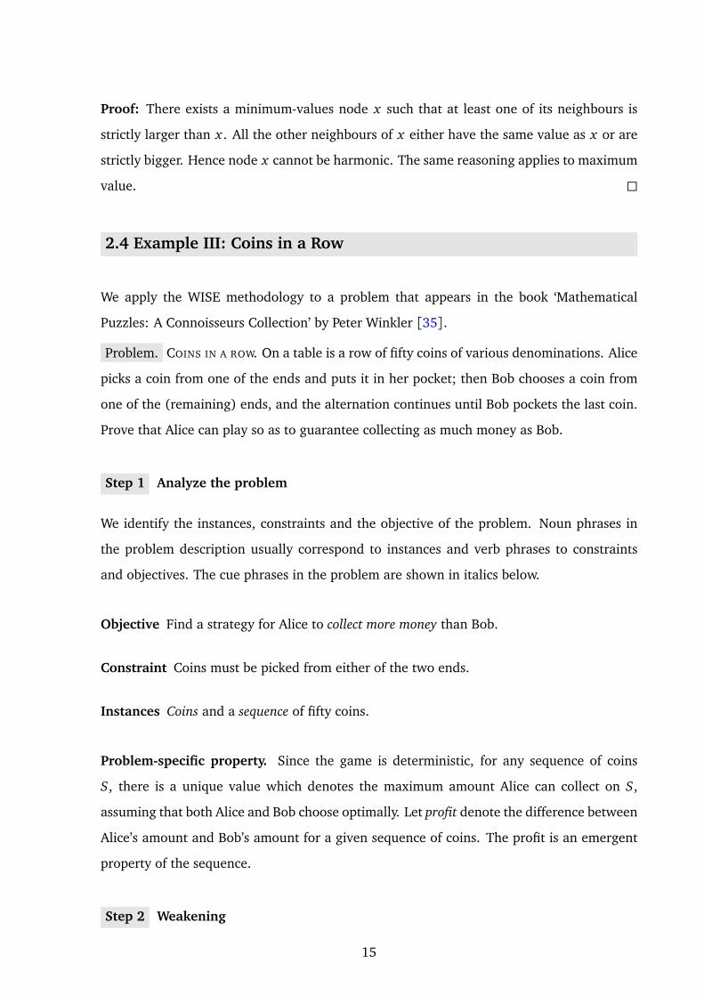
Problem. COINS IN A ROW. On a table is a row of fifty coins of various denominations. Alice
picks a coin from one of the ends and puts it in her pocket; then Bob chooses a coin from
one of the (remaining) ends, and the alternation continues until Bob pockets the last coin.
Prove that Alice can play so as to guarantee collecting as much money as Bob.
Step 1 Analyze the problem
We identify the instances, constraints and the objective of the problem. Noun phrases in
the problem description usually correspond to instances and verb phrases to constraints
and objectives. The cue phrases in the problem are shown in italics below.
Objective Find a strategy for Alice to collect more money than Bob.
Constraint Coins must be picked from either of the two ends.
Instances Coins and a sequence of fifty coins.
Problem-specific property. Since the game is deterministic, for any sequence of coins
S, there is a unique value which denotes the maximum amount Alice can collect on S,
assuming that both Alice and Bob choose optimally. Let profit denote the difference between
Alice’s amount and Bob’s amount for a given sequence of coins. The profit is an emergent
property of the sequence.
Step 2 Weakening
15

Weaken the instance. One way to weaken the input sequence is to restrict the values of
coins to 1s and 0s. Zeroes and ones are extremal because they are the smallest two non-
negative values. A sequence of all zeroes or all ones is also extremal, but this makes the
problem trivial.
Weaken the objective. There are many options to relax the objective or constraints: Can
Alice pick the largest coin always? Can Alice force Bob to pick a particular coin? Can Alice
collect at least half the amount as Bob?
Step 3 Identify a candidate problem
Candidate problem. Given a sequence consisting only zeroes and ones, find a strategy for
Alice to maximize her profit.
Step 4 Solving a candidate problem
This is the step in which extremality is most useful. We would like to identify problem-
specific extremal instances of the candidate problem which can be used to get some insight
into the problem.
Here is an extremal instance based on the emergent property profit: Which configura-
tion consisting of 1s and 0s gives the maximum profit for Alice? The instance is not hard to
construct since at each turn Alice should be able to pick 1 but not Bob:
0 1 10 0 0 0 0 0 01 1 1 1 1 1
In the above example it is easy to see that Alice can pick all the 1s and Bob gets zero.
So the gain for this sequence is maximum over all sequences of the same length.
If 1s and 0s appear in alternate positions, Alice can always pick all the 1s.
0o
1e
1e
0o
0o
0o
0o
0o
0o
0o
1e
1e
1e
1e
1e
1e
Key idea. In general, Alice can pick all the numbers that are in positions of the same
parity, regardless of the values of the coins. Notice how we made this observation simply
by solving the right extremal problem: that of alternate ones and zeroes.
Step 5 Extend the solutions
Near extremal instance: Alternate 1s and 0s except for one position. Alice can win by
collecting 1s if x is less than the number of ones. Otherwise, she can win by collecting x .
16

By generalizing this idea, we see that Alice has a winning strategy: Alice first sums up all
the coins in even positions and all the coins in odd positions. Then, she will pick up all
coins of the same parity that gives her a larger sum.
0o
1e
1e
xo
0o
0o
0o
0o
0o
0o
1e
1e
1e
1e
1e
1e
Sol. Alice either picks all the numbers in even positions or odd positions (whichever is
greater).
Remark. If the sequence is of odd length, then there is no winning strategy for either Alice
or Bob. For example, if the sequence is 0-1-0, then Alice loses. If the sequence is 1-0-0,
then Bob loses.
2.5 Example IV: Grid Minimum
This problem is taken from the textbook by Klienberg-Tardos [21]. GRID MINIMUM is the
last problem in the chapter on divide-and-conquer technique.
Problem. Let G be an n× n grid graph. Each node v in G is labelled by a real number xv;
you may assume that all these labels are distinct. A node v of G is called a local minimum
if the label xv is less than the label xw for all nodes w that are joined to v by an edge. You
are given the grid graph G, but the labelling is only specified in the following implicit way;
for each node v, you can determine the value xv by probing the node v. Show how to find
a local minimum of G using only O(n) probes to the nodes of G. (G has n2 nodes.)
Step 1 Analyze the problem
We first identify the instances of the problem.
• Instances in the problem: Grid graph with values.
• Extremal instances
– An 1× n grid graph (extremality in structure.)
– A grid graph with only one node that is a local minimum (extremality in values.)
Step 2a Weakening the instance
17
Let us consider the extremal instance when the grid graph is of size 1× n. This means the
graph is just a path.
Step 3 Identify a candidate problem
The candidate problem is as follows: What is the least number of queries in which we can
find a local minimum on a path?
Step 4 Solving the candidate problem
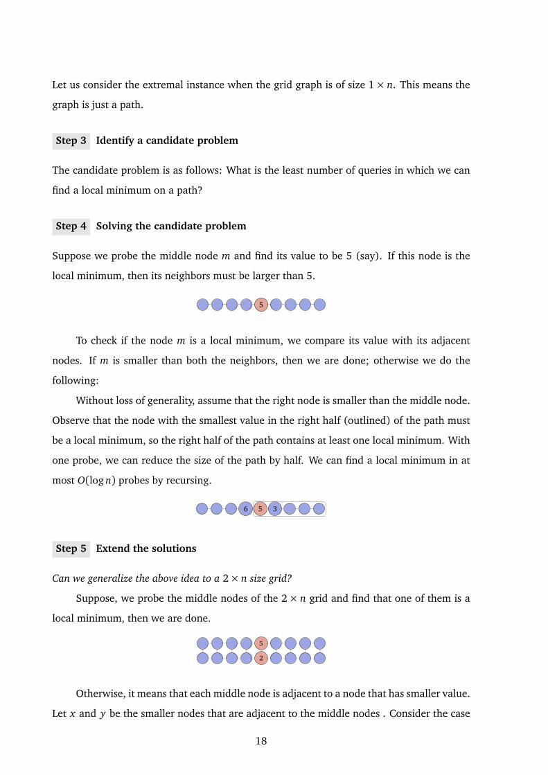
Suppose we probe the middle node m and find its value to be 5 (say). If this node is the
local minimum, then its neighbors must be larger than 5.
5
To check if the node m is a local minimum, we compare its value with its adjacent
nodes. If m is smaller than both the neighbors, then we are done; otherwise we do the
following:
Without loss of generality, assume that the right node is smaller than the middle node.
Observe that the node with the smallest value in the right half (outlined) of the path must
be a local minimum, so the right half of the path contains at least one local minimum. With
one probe, we can reduce the size of the path by half. We can find a local minimum in at
most O(log n) probes by recursing.
56 3
Step 5 Extend the solutions
Can we generalize the above idea to a 2× n size grid?
Suppose, we probe the middle nodes of the 2× n grid and find that one of them is a
local minimum, then we are done.
2
5
Otherwise, it means that each middle node is adjacent to a node that has smaller value.
Let x and y be the smaller nodes that are adjacent to the middle nodes . Consider the case
18
2
5
3
6
1
4
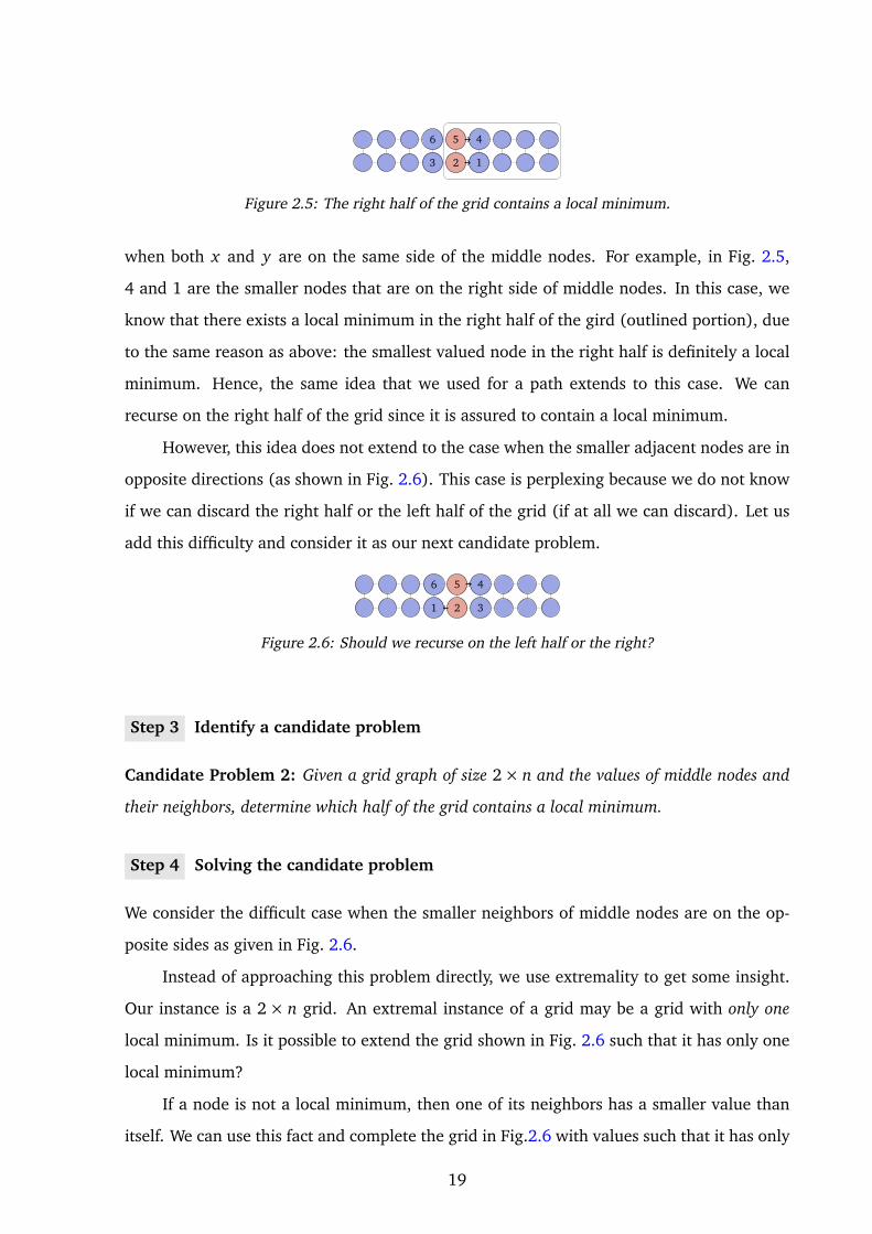
Figure 2.5: The right half of the grid contains a local minimum.
when both x and y are on the same side of the middle nodes. For example, in Fig. 2.5,
4 and 1 are the smaller nodes that are on the right side of middle nodes. In this case, we
know that there exists a local minimum in the right half of the gird (outlined portion), due
to the same reason as above: the smallest valued node in the right half is definitely a local
minimum. Hence, the same idea that we used for a path extends to this case. We can
recurse on the right half of the grid since it is assured to contain a local minimum.
However, this idea does not extend to the case when the smaller adjacent nodes are in
opposite directions (as shown in Fig. 2.6). This case is perplexing because we do not know
if we can discard the right half or the left half of the grid (if at all we can discard). Let us
add this difficulty and consider it as our next candidate problem.
2
5
1
6
3
4
Figure 2.6: Should we recurse on the left half or the right?
Step 3 Identify a candidate problem
Candidate Problem 2: Given a grid graph of size 2× n and the values of middle nodes and
their neighbors, determine which half of the grid contains a local minimum.
Step 4 Solving the candidate problem
We consider the difficult case when the smaller neighbors of middle nodes are on the op-
posite sides as given in Fig. 2.6.
Instead of approaching this problem directly, we use extremality to get some insight.
Our instance is a 2× n grid. An extremal instance of a grid may be a grid with only one
local minimum. Is it possible to extend the grid shown in Fig. 2.6 such that it has only one
local minimum?
If a node is not a local minimum, then one of its neighbors has a smaller value than
itself. We can use this fact and complete the grid in Fig.2.6 with values such that it has only
19

one local minimum. One such extremal case is shown in Fig. 2.7, where node 1 is the only
local minimum.
2
5
17 16 14 1 3 8 11 12
18 15 13 6 4 7 9 10
Figure 2.7: Node 1 is the only local minimum.
The local minimum has appeared on the left side of the grid graph. We observe that
no matter how we try to fill up the values for the remaining nodes in Fig. 2.6, we always
end up with a local minimum on the left side of grid graph. So in some sense, the middle
node 2 seems to have more influence than middle node 5.
Key Fact. Node 2 is the minimum node among the middle nodes 2 and 5.
We reason why the local minimum always appears on the left side of the grid graph
shown in Fig.2.6: Suppose node 1 is a local minimum, then we are done. Otherwise,
let node l be the minimum valued node in the left half of the graph (outlined portion in
Fig. 2.7). The node l is less than all the nodes in the left half of the grid graph including
the middle nodes 2 and 5. Therefore, node l is a local minimum. So in either case, we get
a local minimum on the left side of the grid graph.
Using the above observation, we can now answer candidate problem 2. Suppose we
are given a 2×n grid with middle nodes a and b. Without loss of generality, assume va < vb.
Let x be the neighbor of node a with vx < va. Then there always exists a local minimum in
that half of the grid graph that contains node x .
Step 5 Extend the solutions
The solution to the 2× n grid gives enough insight to solve the original problem. We give a
divide-and-conquer algorithm below:
Sol. Given an n×n grid, we probe all middle nodes and check if one of the middle nodes is
a local minimum. If this is true, then we are done. Otherwise, we find the minimum valued
node among the middle nodes (call this minimum valued node m). Since m is not a local
minimum, there exits a node x , either to m’s right or left such that vx < vm. Let G′ be the
half of the grid than contains vx . G′ is a n× n/2 grid. Apply the probing procedure again
to G′ and partition it into two halves. Let G′′ be the half that contains the local minimum.
Recurse on G′′. This is the divide-step of the algorithm that uses only 3n/2 probes and
20

reduces the problem into an instance of size n/2× n/2. The associated recurrence relation
is
T (n) = T (n/2) + 3n/2
which implies that the algorithm runs in linear time.
2.6 Discussion
We notice a common feature in all the solutions obtained using WISE. In every problem that
we have discussed, the use of WISE methodology is invisible in the final solution. We use
the methodology only as a scaffold to obtain insight into the problem. This aspect of WISE
is prevalent in all the applications we discuss. The invisibility of WISE methodology makes
it different from other design techniques like greedy, divide and conquer and dynamic pro-
gramming. The solutions obtained using these techniques usually have a signature of the
technique that was used to solve them.
21

22

Chapter 3
Constructing Counterexamples using
WISE
3.1 Introduction
Greedy, divide-and-conquer, recursion, dynamic programming are some of the prominent
algorithm design techniques that are taught at undergraduate level. Counterexamples of-
ten crop up in the context of greedy algorithms because they are useful in discarding naïve
approaches. While there is a method to prove a greedy algorithm correct (‘exchange argu-
ment’) (Chap. 10, [6]), to the best of our knowledge, there is no method that is specifically
aimed at designing counterexamples for greedy algorithms. Students simply rely on their
intuition or search for counterexamples by trying small cases.
Broadly, the task of constructing counterexamples is as follows. We are given an op-
timization problem P and a greedy algorithm that is purported to solve P. We need to
construct an instance of P on which the greedy algorithm fails (Fig. 3.1). We present a
technique called the Anchor method based on the extremality principle discussed in the first
chapter. The method is a specific application of the WISE methodology. We limit the scope
of our work to simple greedy approaches and the scope of our problems to graph theoretic
problems on unweighted graphs. We show that anchor method works on many well-known
problems. The specific list of problems can be found in Table 3.1.
Remark. Preliminary version of this work appears in [24].
23

Task T
OptimizationProblem P
GreedyAlgorithm A
GreedyCounterexample C
Original Task
Figure 3.1: A greedy counterexample is an instance of P on which the greedy algorithm fails.
3.2 Definitions
In this section, we prepare the ground by first giving a few definitions.
3.2.1 Definitions related to graphs
A graph is an ordered pair G = (V, E) where V is the set of vertices and E the set of pairs of
vertices called edges. The pair of vertices in an edge are unordered so edge (u, v) is same
as (v, u). For an edge e = (u, v) we say e is incident on vertex u and v. Vertices u and v are
also called endpoints of e. The degree of a vertex is the number of edges incident on it.
A subgraph of G is a graph H such that V (H) ⊆ V (G) and E(H) ⊆ E(G) and the
assignment of endpoints to edges in H is the same as in G. A graph H is a proper subgraph
of G if H is subgraph of G and H 6= G.
We delete a vertex v from G = (V, E) by removing v from V and removing all the edges
that are incident on v from E.
3.2.2 Definitions related to problems
In a constraint problem P, we are given a graph G and a set of constraints as input. A solution
to the constraint problem P is a subgraph of G that satisfies the given set of constraints.
An optimization problem is a constraint problem in which each solution is assigned a
value (a number) and the objective is to find a solution with the optimal value OPT. The
optimization problem is either a minimization or maximization problem.
MIS Problem. Let G = (V, E) be a graph. An independent set in G is a vertex set S ⊆ V
such that no two vertices in S have an edge between them in E. The problem is to find an
24

independent set in G with maximum number of vertices. See Fig. 3.2.
a b
de
c
Figure 3.2: In the graph shown, S = a, c is a maximum independent set (MIS). So, OPT=2.
Every independent set in G is a solution to the problem. The value of a solution is the
number of vertices in it. The MIS problem is therefore an optimization problem.
3.2.3 Definitions related to algorithms
An algorithm for an optimization problem is a well-defined procedure which finds a solution
to the problem (not necessarily the optimal).
Greedy algorithm. The greedy algorithm works by ‘making the choice that looks best at
the moment’ [21]. We do not dwell on what exactly qualifies as a greedy algorithm. The
notion of locally-best choice will appeal only intuitively.
Greedy algorithm for MIS. Consider the following greedy algorithm to solve the MIS prob-
lem. When a vertex is picked, we are prohibited from picking its neighbors. Since we want
to pick as many vertices as possible, intuitively it is reasonable to pick a vertex with least
degree first [28].
Algorithm 3.2.1: MIS(G)
Input: Graph G
Output: An independent set S from graph G
Initially the set S is empty.
1 : Pick a vertex v from G with the least degree.
Add v to S.
2 : Delete v and all its neighbors from G.
3 : Repeat the above two steps until G has no vertices.
4 : Report S as the solution
Weak algorithm. We define a weak algorithm to be an algorithm that works by making an
arbitrary choice at each moment.
25

3.2.4 Definitions related to counterexamples
Counterexample. For a given optimization problem and an algorithm, a counterexample is
a problem instance on which the algorithm produces a non-optimal solution.
Plausible and definitive counterexamples. If more than one choice looks best at a given
moment, the greedy algorithm picks one of the best choices arbitrarily. Hence, an algorithm
could have multiple execution paths for the same input instance. We call an input instance
a plausible counterexample if one of the execution paths leads to a wrong answer. Similarly,
an input instance is called a definitive counterexample if every possible path of execution
leads to a wrong answer. It is a convention to treat plausible counterexamples as valid
counterexamples. So for the rest of the chapter, we refer to plausible counterexamples
simply as counterexamples.
Weak and greedy counterexamples. A weak counterexample is a counterexample to a
weak algorithm. Similarly, a greedy counterexample is a counterexample to a greedy algo-
rithm.
Goodness ratio. The goodness ratio of a counterexample is a measure that compares the
value of the optimal solution to the value of the solution obtained by the algorithm. We
define it as follows: Suppose I is an input to an algorithm A. Let OPT be the value of the
optimal solution to I and ALG be the value of the solution returned by the algorithm A.
The goodness ratio of the input I is defined as the ratio of OPT to ALG, for maximization
problems. For minimization problems, it is the ratio of ALG to OPT. For example, for the
input shown in Fig. 3.8 OPT=3 and ALG=2, so the goodness ratio is 1.5.
a
b
c
K3
Figure 3.3: A counterexample to Alg. 3.2.1 for the MIS problem. A dark edge indicates that there
are edges from the high degree vertex to all the three vertices in K3. The central vertex has degree
3. Vertices a, b and c have degree 4 each. Each vertex in K3 has degree 5. So the greedy algorithm
picks the central vertex first and then picks one vertex from K3. The maximum independent set is
actually a, b, c. Hence, the greedy algorithm picks 2 vertices, while the optimal algorithm picks 3.
26

We usually express goodness ratio in an asymptotic sense i.e. as a function of the
number of vertices in the counterexample.
General Counterexample. A general counterexample is a graph family of counterexamples
such that for any given number k, we can find a graph in the family with larger than
k vertices. A general counterexample is said to be tight if it achieves the best possible
goodness ratio (in the asymptotic sense).
3.2.5 Definitions related to solutions
Local solution. Let G be the input graph of a maximization problem P. A solution to P
is said to be local if it is not a proper subgraph of any other solution in G. Likewise, a
solution to a minimization problem P ′ involving input graph G′ is said to be local if no
proper subgraph of it is a solution in G′.
Discrepancy. Suppose G is the input graph of an optimization problem. Let S1 and S2 be
two local solutions in G whose values are s1 and s2, respectively. Without loss of generality,
assume that s1 >= s2. The ratio s1/s2 is called the discrepancy of the graph G.
3.3 Anchor Method
The Anchor method consists of three main steps which are briefly described below.
Step 1. Construct a counter-example for the weak algorithm.
(Tip: Try graphs with high discrepancy.)
Step 2. Observe how the weak algorithm fails.
Step 3. Extend the weak counterexample to a greedy counterexample.
(Tip: Try attaching graphs with low discrepancy.)
3.4 Anchor Method using MIS as an Illustrative Example.
Step 1 Analyze the task
The scope of the method is limited to graph-theoretic optimization problems and greedy
algorithms. We make sure that the given problem is within the scope by verifying if the
given problem is an optimization problem as defined in Sec. 3.2.2.
27

The attributes of the MIS problem are as follows.
• Input. A graph G = (V, E).
• Solution. A set of vertices S ⊆ V . Hence, the solution is a sub-graph of G as required.
• Constraints. A set of vertices S must be independent.
• Value of a solution. The number of vertices in S.
• Greedy choice. Pick the least-degree vertex first.
Clearly, MIS problem is an optimization problem and belongs to the scope of problems
for which the method is applicable.
Task. To construct a counterexample to the greedy algorithm for the MIS problem.
Step 2 Weakening Step
Our objective is to construct a counterexample to a given greedy algorithm. We first ask if
we can achieve a simpler objective: Can we construct a counterexample for an algorithm
that does not make any greedy choices?
Task T1
OptimizationProblem P
WeakAlgorithm A′
WeakCounterexample
C ′
Weakening Step.
Figure 3.4: Instead of solving the original task directly, we first pose an easier task. The optimization
problem is kept the same but the algorithm is changed from greedy to a weak algorithm.
Recall that a weak algorithm is obtained from the greedy algorithm by replacing the
greedy choice with an arbitrary choice. The assumption is that the weak counterexample
gives insight into the structure of the greedy counterexample. We call the weak counterex-
ample an anchor.
28

The algorithm Alg. 3.2.1 picks the vertices in increasing order of degree, so the corre-
sponding weak algorithm picks vertices in arbitrary order.
So now the weaker task is to construct a counterexample for the following algorithm:
Algorithm 3.4.1: MIS-WEAK(G)
Input: Graph G
Output: An independent set S from graph G
Initially the set S is empty.
1 : Pick a vertex v from G.
Add v to S.
2 : Delete v and all its neighbors from G.
3 : Repeat the above two steps until G has no vertices.
4 : Report S as the answer
Weak Counterexample. A weak counterexample is an instance on which the weak
algorithm fails assuming the worst possible execution or, in other words, when choices are
made in an adversarial manner (e.g. Fig. 3.5).
Remark. In the WISE methodology in Sec. 2.1, we mentioned that one may need to pose
multiple weaker problems and then identify the problems to be solved first. If the weak-
ening step has multiple weaker tasks, we would have had to identify a task to solve first.
Since there is only one weaker task (as described above), the identification step is trivial.
Step 3 Solving the candidate problem
In this step, we construct a weak counterexample. There could be several weak counterex-
amples for a given weak algorithm. It helps to construct multiple weak counterexample
with high discrepancy.
A counterexample to Alg. 3.4.1 is shown in Fig. 3.5.
a
b
c
Figure 3.5: A counterexample to the weak algorithm for the MIS problem. A star graph with three
outer vertices.
29

The weak algorithm could pick the central vertex first and get an independent set of
size 1, whereas the maximum independent set has size 3 (a, b, c). So this is our weak
counterexample.
In Sec. 3.5, we explain how extremality can be used to pick the ‘good’ weak coun-
terexamples.
Step 4 Extending the weak counterexample
Task T2
Weak Coun-terexample C ′
Anchor
GreedyAlgorithm A
GreedyCounterexample C
Extending Step.
Figure 3.6: In the extend step, we use the weak counterexample from the previous step to guide the
process of constructing a greedy counterexample.
In this step, we extend the weak counterexample to a greedy counterexample (Fig. 3.6).
We do so following two steps:
1. First, we observe how the weak algorithm behaves on the weak counterexample.
Then we ask ourselves, what would have to happen if the greedy algorithm were to
go wrong in the same way as the weak algorithm? We isolate this ‘bad structure’ and
call it the anchor.
2. We attach a graph to the anchor to obtain a greedy counterexample. The attached
graph is called the auxiliary structure. The term is meant to suggest that this structure
performs a supporting role to the anchor.
In Sec. 3.5, we explain how extremality can be helpful in picking the right auxiliary
structure.
Building an anchor for the MIS problem. In the weak counterexample (Fig. 3.5), the
central vertex has the highest degree. We want the greedy algorithm to go wrong in the
30

same way as the weak algorithm. We know that the greedy algorithm would pick the
central vertex in the above graph first if the central vertex had the lowest degree somehow.
We capture this intuition in the anchor (Fig. 3.7). The anchor is a skeleton that captures the
essence of a possible greedy counterexample. It serves as a starting point for constructing
a counterexample to the greedy algorithm.
Notation. We use symbols and to indicate a vertex we wish were of high degree
and low degree, respectively.
Figure 3.7: The anchor obtained from the weak counterexample. If the central degree had the lowest
degree somehow, then the greedy algorithm would fail in the same way as the weak algorithm.
Adding an auxiliary structure. Each high degree vertex needs to be connected to at least
3 vertices in order to exceed the low degree central vertex. Let Kn denote a complete
graph with n vertices. Attaching the auxiliary graph K3 gives a counterexample as shown
in Fig. 3.8.
a
b
c
K3
Figure 3.8: A counterexample to Alg. 3.2.1 for the MIS problem. A dark edge indicates that there
are edges from the high degree vertex to all the three vertices in K3. The central vertex has degree
3. Vertices a, b and c have degree 4 each. Each vertex in K3 has degree 5. So the greedy algorithm
picks the central vertex first and then picks one vertex from K3. The maximum independent set is
actually a, b, c. Hence, the greedy algorithm picks 2 vertices, while the optimal algorithm picks 3.
3.5 Role of Extremality
In this section, we explain how to pick useful weak counterexamples and auxiliary struc-
tures based on the principle of extremality. We may have to try multiple weak counterexam-
31

ples and auxiliary structures before hitting upon the right combination that gives a greedy
counterexample. The following tips are helpful in picking the right structures:
Tip for choosing the weak counterexample. Pick those graphs which have the highest
discrepancy.
Tip for choosing the auxiliary structure. Pick those graphs which have the least discrep-
ancy.
Usually, the extremal graphs that have the highest or the least discrepancy are easy to
find by trial and error. They are usually composed of simple structures like the ones shown
in Table 1.2.
Let us apply this tip to picking a weak counterexample for the MIS problem. We want
to choose such a graph which has two local solutions of different size. Searching through
the generic extremal graphs (Table 1.2) we find that the star graph has this property.
r
. . .1 2 n
Figure 3.9: A weak counterexample and the corresponding anchor. There are two local solutions in
the counterexample, one of size 1 and the other of size n. The discrepancy is therefore O(n), which
is the highest possible discrepancy for the MIS problem.
Let us pick an auxiliary structure for the MIS problem based on discrepancy.
Kn
(a)
In
(b)
Figure 3.10: Two graphs with discrepancy 1. In the complete graph (a), any local solution has size
1. In an independent set graph (b) any local solution has size n. Hence, Kn and In are extremal
graphs with the least discrepancy for the MIS problem. Again, both these graphs were among the
generic extremal graphs shown in Table 1.2.
Attaching the auxiliary structure Kn to the anchor gives us a general counterexample
(Fig. 3.11). This counterexample has a goodness ratio of O(n) which is also tight.
32

Kn
. . .1 2 n
Figure 3.11: A general counterexample to Alg. 3.2.1 for the MIS problem with O(n) goodness ratio.
The greedy algorithm picks 2 independent vertices, while the optimal algorithm picks n vertices.
Problem Anchor Aux. St. G. Ratio Best Ratio
INDEPENDENT SET Star Kn O(n) O(n)
VERTEX COVER Star Centipede 2 log n
MATCHING Paths Kn,n 2 2
MAXLEAF Path Binary tree 2 2
MAXCUT Kn,n Kn,n 2 2
NETWORK FLOW - Paths O(p
n) O(p
n)
TRIANGLE-FREE - Kns 4/3 O(log n)
DOMINATING SET Paths Paths 1.5 O(log n)
Table 3.1: Applicability of anchor method on common graph-theoretic problems. The anchors and
the auxiliary structures of most counterexamples come from simple extremal graphs (Table 1.2).
Symbol - indicates that the anchor is problem-specific. Descriptions of the problems and the corre-
sponding greedy algorithms can be found in Sec. 3.6.
33
3.6 Additional Examples
We show the applicability of the anchor method on many classic problems from graph
theory. Most of the problem descriptions along with their applications can be found in
standard texts like [13, 34].
3.6.1 Minimum Vertex Cover Problem
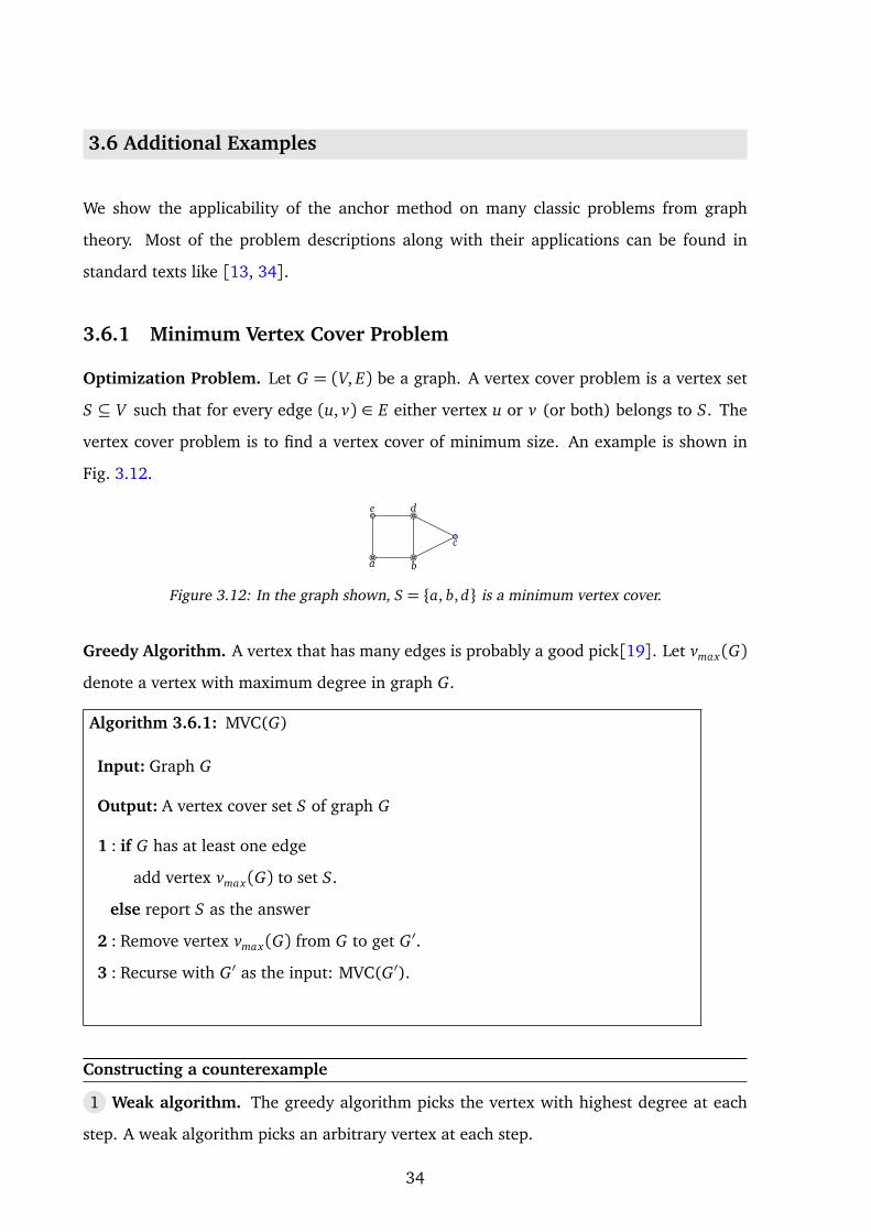
Optimization Problem. Let G = (V, E) be a graph. A vertex cover problem is a vertex set
S ⊆ V such that for every edge (u, v) ∈ E either vertex u or v (or both) belongs to S. The
vertex cover problem is to find a vertex cover of minimum size. An example is shown in
Fig. 3.12.
a b
de
c
Figure 3.12: In the graph shown, S = a, b, d is a minimum vertex cover.
Greedy Algorithm. A vertex that has many edges is probably a good pick[19]. Let vmax(G)
denote a vertex with maximum degree in graph G.
Algorithm 3.6.1: MVC(G)
Input: Graph G
Output: A vertex cover set S of graph G
1 : if G has at least one edge
add vertex vmax(G) to set S.
else report S as the answer
2 : Remove vertex vmax(G) from G to get G′.
3 : Recurse with G′ as the input: MVC(G′).
Constructing a counterexample
1 Weak algorithm. The greedy algorithm picks the vertex with highest degree at each
step. A weak algorithm picks an arbitrary vertex at each step.
34

2 Weak counterexample. A star graph is a simple extremal graph on which the weak
algorithm fails. There are two local solutions in the star graph (Fig. 3.13):
• S1 : The root node r.
• S2 : The vertices labelled 1 to n.
The weak algorithm could pick the leaf nodes and find solution S2, whereas S1 is the
minimum vertex cover.
r
. . .1 2 n
Figure 3.13: A weak counterexample for the vertex cover problem. The discrepancy of the graph is
O(n). The star graph also has the highest discrepancy among all the weak counterexamples.
3 Building an anchor. To build an anchor we ask ourselves: “What would have to happen
if the greedy algorithm were to fail in the same way as the weak algorithm?” The greedy
algorithm pick the highest degree vertex first. So if somehow the leaf nodes had high degree
and the root node had the lowest degree then the greedy algorithm would fail in the same
way as the weak algorithm. We capture this intuition by an anchor (Fig. 3.14).
r
. . .1 2 n
Figure 3.14: An anchor corresponding to the weak counterexample. We wish the root node were of
low degree and the leaf nodes were of high degree.
4 Adding the auxiliary structure. We need to find an auxiliary structure that can be
attached to the anchor. As mentioned in Sec. 3.5, it helps to first look at simple extremal
graphs with low discrepancy. Fig. 3.15 shows a few such graphs.
In
(a)
Kn
(b) (c)
PnC tn
(d)
Figure 3.15: Four simple graphs with discrepancy 1. The value of any local solution (vertex cover)
in each graph from left to right is 0, n− 1, n/2 and n, respectively.
35

We try to extend the anchor to a greedy counterexample by trying to attach each
one of the graphs shown in Fig. 3.15. Attaching a path of length n + 2 gives a greedy
counterexample (Fig. 3.16). Similarly, attaching a centipede of length n+ 3 gives a greedy
counter example (Fig. 3.17). For Kn, attaching one Kn makes the vertices in Kn itself as the
highest degree vertices so we try attaching two Kns, which does the trick (Fig. 3.18). There
does not seem to be any way of extending by attaching In.
. . .1 2 n
Figure 3.16: A counterexample for vertex cover. The auxiliary path attached has length n+ 2. Each
leaf node of the anchor has degree n+3. The greedy algorithm picks all the leaf nodes of the anchor
and alternate nodes from the path. This gives a vertex cover of size ≈ 1.5n. The optimal solution is
to pick the root node of the anchor and all the vertices in the attached path. This gives a minimum
vertex cover of size n+ 3. Hence the goodness ratio of this counterexample is limn→∞1.5nn+3= 1.5.
. . .1 2 n
Figure 3.17: A counterexample for vertex cover with goodness ratio 2. The centipede attached has
length n+ 3.
Kn
Kn
. . .1 2 n
Figure 3.18: A counterexample for vertex cover using Kns as an auxiliary structure. The goodness
ratio of the counterexample is 1.5.
36

3.6.2 Bipartite Matching
A graph G = (V, E) is bipartite if the vertex set can be partitioned into two sets A and B such
that no edge in E has both endpoints in A or B alone.
A set of edges M is called a matching if M ⊆ E and every vertex in G is an endpoint of
at most one edge in M . A vertex is said to be matched if it is an endpoint of some edge in
M ; if not the vertex is said to be unmatched.
Optimization Problem. Let G = (V, E) be a bipartite graph. The bipartite matching prob-
lem (MBM) is to find a matching M of maximum size in G
A B
Figure 3.19: In the graph above, the dark edges form a matching of size 5.
Greedy Algorithm. A vertex with degree one has to necessarily be matched to its neighbor
if it has to participate in the matching. In general, a vertex with fewer neighbors has fewer
choices and therefore more critical.
Notation. Let vmin denote the vertex with minimum non-zero degree in graph G and
37

umin denote the vertex with minimum degree adjacent to vmin.
Algorithm 3.6.2: MM(G)
Input: Graph G
Output: A matching M from graph G
Initially the matching set M is empty.
1 : if graph G has no edges
report M as the matching set.
2 : Add the edge (vmin, umin) to the set M .
3 : Remove the vertices vmin and umin from G
to get the subgraph G′.
4 : Recurse on the graph G′: MM(G′)
Constructing a counterexample
1 Weak algorithm. The weak algorithm picks edges in any order and includes them in
matching set M .
2 Weak counterexample. A path of four nodes in the simplest instance on which the
weak algorithm fails. A general counterexample is obtained by making many copies of
P4, as shown in Fig. 3.20. The weak algorithm could pick just the middle edges, while the
optimal algorithm picks the first and the last edge of each path. Hence, the optimal solution
can be twice as good as the weak algorithm’s solution.
3 Building an anchor. The greedy algorithm would behave like the weak algorithm if the
end points of each path were of high degree. The anchor captures this intuition (Fig. 3.21).
4 Adding the auxiliary structure.
We attach an auxiliary structure (K2,2) to each of the high degree nodes. If we start
with the anchor obtained by the general weak counterexample (Fig. 3.22) we can get a
tight counterexample with goodness ratio 2 (Fig. 3.23). Observe that Kn,n has the least
discrepancy since all the local solutions have size n.
38

...
Figure 3.20: A general weak counterexample for the bipartite matching problem with goodness ratio
2.
Figure 3.21: The anchor for bipartite matching is obtained by replacing the end vertices of P4 with
high degree vertices. We want the greedy algorithm to pick the middle edge. This would happen if
the end vertices were of high degree and the middle nodes were of low degree.
...
Figure 3.22: The anchor obtained from the
general weak counterexample.
...
K2,2
Figure 3.23: A tight counterexample for the
bipartite matching problem. The shaded ver-
tices have degree three. The goodness ratio
of the graph is 2.
39

a
b
d
e c
a
b
d
e c
a
b
d
e c
Figure 3.24: Two spanning trees for the graph given on the left: one with 3 leaves and the other
with 2 leaves.
3.6.3 Maximum leaf spanning tree
Optimization Problem. Given a graph G = (V, E), the maximum leaf spanning tree prob-
lem (MLS) is to find a spanning tree T in G that has maximum number of leaves; where
leaves are vertices with degree 1. An example is shown in Fig. 3.24.
Greedy Algorithm. We would like to grow the tree along vertices that branch out well. One
strategy is to grow the tree along a vertex which has the maximum number of neighbors
not in the tree [17].
Notation. For a vertex v in tree T , let N ′(v) denote the set of neighbors of v not in T .
Algorithm 3.6.3: MLS(G)
Input: A connected graph G
Output: A spanning tree T of graph G
Tree T initially has only the vertex vmax(G).
repeat
1 : Pick a vertex u in T such that the
size of the set N ′(u) is maximized.
2 : Grow the tree T by attaching
vertices in N ′(u) to u.
until the tree T has all the vertices in G
Constructing a counterexample
1 Weak algorithm. In the greedy algorithm, we grow the tree T along the vertex that has
maximum number of neighbors outside the tree. Consider the weak algorithm that does
not exercise this choice and instead grows the tree along any arbitrary vertex.
2 Weak counterexample. None of the simple extremal graphs is a counterexample, so
we need to construct a weak counterexample by trial and error. An instance where the
40

r
l
Figure 3.25: A weak counterexample for the max-leaf spanning tree problem. The optimal solution
is to start with the node r and pick all its neighbors. The weak algorithm could start with the
leftmost node and pick a spanning tree having only two leaves.
Figure 3.26: If the greedy algorithm has to fail like the weak algorithm then the leftmost node must
have high degree and all the nodes of the path must be leaves of some tree.
weak algorithm could perform poorly is given in Fig. 3.25. The optimal algorithm would
pick the vertex with the highest degree r and obtain a spanning tree having |V | − 1 leaves.
If the weak algorithm picks vertex l first, it could end up with a spanning tree having only
two leaves (as indicated with dark background).
3 Building an anchor.
The key to designing the weak counterexample was to make the algorithm select a
long path of vertices which should have been selected as leaves. We want the greedy
algorithm to mimic that behaviour? We make the greedy algorithm start from the first node
by increasing its degree.
4 Adding the auxiliary structure. The vertices of this path must be the leaves of some
tree. We need to attach an auxiliary structure such that the vertices on the path become
leaves. The auxiliary structure cannot have a vertex with degree greater than 3 since we
have forced the greedy algorithm to pick the the leftmost vertex in the anchor first. The
complete binary tree serves this purpose. The counterexample is shown in Fig. 3.27.
Figure 3.27: A tight counterexample for max-leaf spanning tree problem with goodness ratio 2.
41

3.6.4 Max Cut
Optimization Problem. Let G = (V, E) be a graph, and S ⊆ V be any subset. Then
E(S, S)de f= (u, v) : u ∈ S and v /∈ S forms a cut. The MAX-CUT problem is as follows. Given
a graph G as input, find S ⊆ V which maximizes the value of |E(S, S)|.
Greedy Algorithm. Suppose E(S, S) is a cut. If moving a vertex from S to S increases the
value of the cut, then we must do so. A greedy strategy is to move a vertex that results in
the largest increase in the value of the cut.
Algorithm 3.6.4: MAXCUT(G)
Input: A graph G = (V, E)
Output: A subset S ⊆ V
Initialize S = V .
repeat
1 : Let v ∈ V be the vertex that results in
the maximum increase in the value of the cut
if moved from S to S (or vice-versa)
2 : Move v from S to S (or vice-versa).
until there is no positive increase in the value of
the cut by moving any vertex.
Constructing a counterexample
1 Weak algorithm. The greedy algorithm moves a vertex that results in the largest
increase in the cut. The weak algorithm could move the vertex that results in the smallest
increase in the cut.
2 Weak counterexample. There are many generic extremal graphs that are counterex-
amples to the weak algorithm. We pick Kn,n since it has the highest discrepancy. There
exists a cut with size n2 but the weak algorithm settles for a cut with size zero.
3 Building an anchor. We want the greedy algorithm to not move the vertices into the
other partition, as shown in Fig. 3.28.
4 Adding the auxiliary structure.
42
A
B
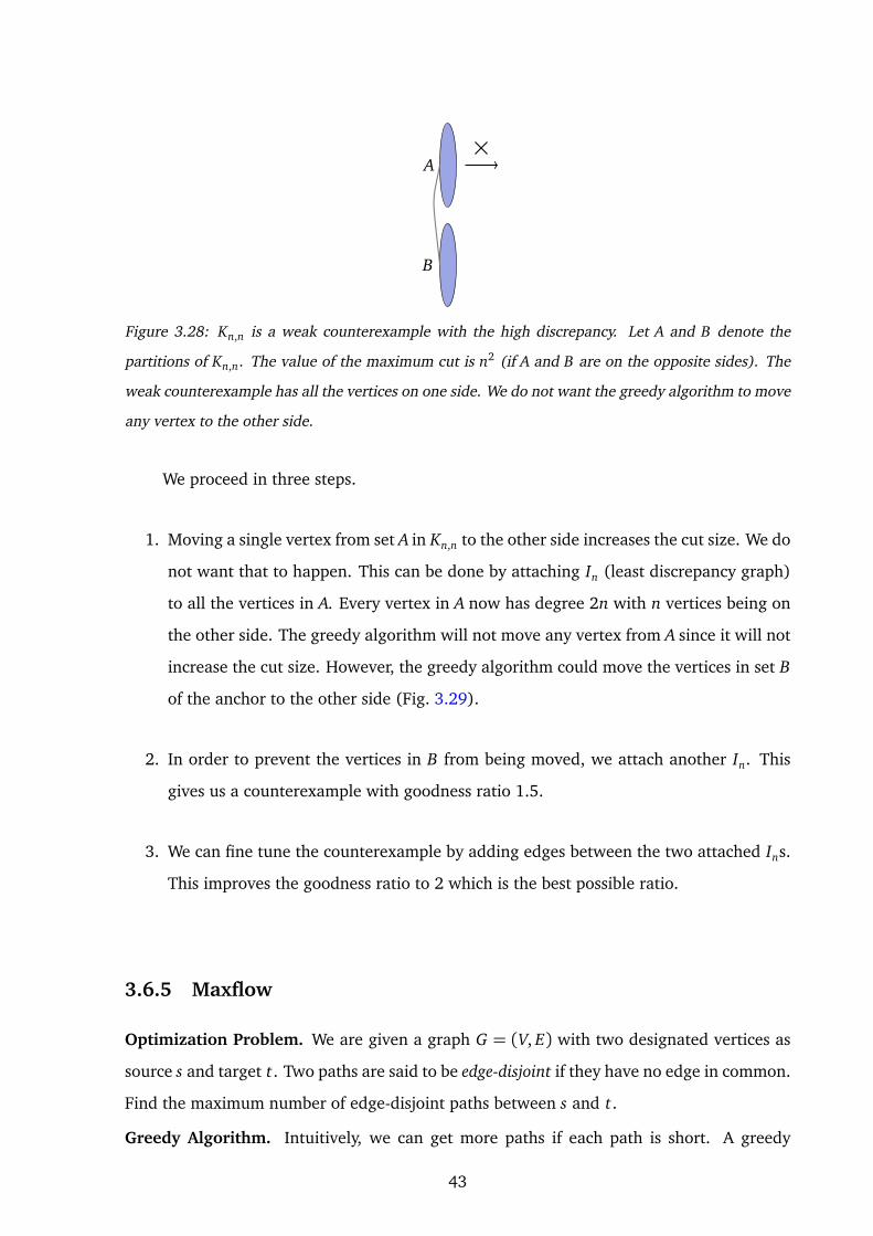
Figure 3.28: Kn,n is a weak counterexample with the high discrepancy. Let A and B denote the
partitions of Kn,n. The value of the maximum cut is n2 (if A and B are on the opposite sides). The
weak counterexample has all the vertices on one side. We do not want the greedy algorithm to move
any vertex to the other side.
We proceed in three steps.
1. Moving a single vertex from set A in Kn,n to the other side increases the cut size. We do
not want that to happen. This can be done by attaching In (least discrepancy graph)
to all the vertices in A. Every vertex in A now has degree 2n with n vertices being on
the other side. The greedy algorithm will not move any vertex from A since it will not
increase the cut size. However, the greedy algorithm could move the vertices in set B
of the anchor to the other side (Fig. 3.29).
2. In order to prevent the vertices in B from being moved, we attach another In. This
gives us a counterexample with goodness ratio 1.5.
3. We can fine tune the counterexample by adding edges between the two attached Ins.
This improves the goodness ratio to 2 which is the best possible ratio.
3.6.5 Maxflow
Optimization Problem. We are given a graph G = (V, E) with two designated vertices as
source s and target t. Two paths are said to be edge-disjoint if they have no edge in common.
Find the maximum number of edge-disjoint paths between s and t.
Greedy Algorithm. Intuitively, we can get more paths if each path is short. A greedy
43

Step 1 Step 2
Kn,n
Kn,n
Step 3
Figure 3.29: We use the anchor as a starting point and add the auxiliary structure in three steps. We
get a tight counterexample with goodness ratio 2.
strategy would be to pick the paths in the order of increasing path lengths.
Algorithm 3.6.5: MAXFLOW(G)
Input: A graph G = (V, E) and two vertices s and t belonging to V .
Output: A collection of disjoint paths from s to t.
repeat
1 : Pick the shortest path P from s to t.
2 : Remove all the edges in P.
until vertex s is disconnected from t.
Constructing a counterexample
1 Weak algorithm. The weak algorithm works like the greedy algorithm, except that
instead of picking the shortest path from s to t it picks any path from s to t at each step.
2 Weak counterexample. It is easy to imagine a graph where picking a long path disrupts
a lot of short disjoint paths. For example, in Fig. 3.30, source s is connected to k vertices.
There exists a flow of size k, but the weak algorithm could pick the long path and get only
a flow of size 1. This graph has discrepancy of O(n).
3 Building an anchor. We want the greedy algorithm to mimic the weak algorithm. This
would happen if the dashed short path in the weak counterexample were somehow longer
than the longest path. In Fig. 3.30 (b), the dashed lines should be longer than the solid
line.
44

4 Adding the auxiliary structure. We replace the dashed lines in the anchor with long
paths of size 2k + 3. This gives us a greedy counterexample (Fig. 3.31). There are O(k2)
vertices in the graph and the maximum flow possible is k. But the greedy algorithm picks
one long path and gives a flow of size 1. Hence, the goodness ratio of the counterexample
is O(p
n), which is the best possible.
s t s t
Figure 3.30: A weak counterexample for the max-flow problem. A flow of O(n) units exists but the
weak algorithm finds a flow of only 1 unit.
s t
Figure 3.31: A tight counterexample for the greedy max-flow algorithm. The counterexample has
goodness ratio of O(p
n).
3.6.6 Triangle Removal Problem
Optimization Problem. A graph is said to be triangle-free if it does not contain K3 as a
subgraph. The triangle removal problem (TR) asks for the minimum set of vertices one
should remove from a graph in order to make it triangle-free. More precisely, given a graph
G = (V, E), find a set F ⊆ V such that G \ F is triangle-free and the size of F is minimum.
An example is shown in Fig. 3.32.
a b
de
c
e
a b
c
Figure 3.32: We can make the above graph triangle-free by just removing vertex d.
45

Greedy Algorithm. We would like to pick vertices whose removal disrupts a large number
of triangles.
Algorithm 3.6.6: TR(G)
Input: Graph G
Output: A vertex set F
Initially set F is empty.
1 : if graph G is triangle-free
report F as the output.
Let u be the vertex in G that is contained
in maximum number of triangles.
2 : Add vertex u to set F
3 : Remove u from G to get a subgraph G′
4 : Recurse on G′: TR(G′).
Constructing a counterexample
1 Weak algorithm. The greedy choice is to remove the vertex which is contained in
maximum number of triangles. The weak algorithm removes any vertex contained in some
triangle.
2 Weak counterexample. Consider a flower which is a graph in which a set of triangles
are connected at a single vertex. The central vertex that can be removed to make the
graph triangle-free. The weak algorithm might end up picking one vertex from each K3
(Fig. 3.33).
3 Building an anchor. The anchor corresponding to the flower has n outer vertices which
are in many triangles.
4 Adding the auxiliary structure. We need the outer vertices to be contained in more
cycles than the central vertex. Attaching three Kns as an auxiliary structure serves the
purpose. Adding edges between each outer vertex and every vertex from Kns gives a greedy
counterexample with approximation ration 4/3 (Fig. 3.33).
46

K n
K n
K n
Figure 3.33: Weak counterexample and a greedy counterexample for the triangle removal problem.
3.6.7 Minimum Dominant Set Problem
Optimization Problem. We are given a graph G = (V, E) as input. A vertex set S is called
dominant if every vertex in G either belongs to S or is a neighbor of a vertex in S. The
minimum dominant set problem is to find a dominant set S of minimum size.
Greedy Algorithm. The problem is closely related to vertex cover and we follow a similar
greedy strategy. A vertex is covered if it is in the dominant set or is a neighbor of a vertex in
the dominant set. We proceed by picking those vertices which cover the maximum number
of vertices at each step.
Algorithm 3.6.7: MINDOM(G)
Input: A graph G
Output: A dominant set S ⊆ V of graph G
Set S is initially empty.
Initially all the vertices are colored white.
repeat
1 : Pick a vertex v which has the maximum number of white neighbors.
2 : Color v and all it’s neighbors black. Add v to S.
until no white colored vertices are left.
Constructing a counterexample
1 Weak algorithm. The greedy algorithm picks the vertex with highest number of uncov-
ered neighbors. The weak algorithm picks any vertex and includes it in the dominant set S
as long as it is not present in S.
2 Weak counterexample. A collection of n paths of length three. The minimum dominant
set has size n, but the weak algorithm could pick all the degree one vertices and get a
47
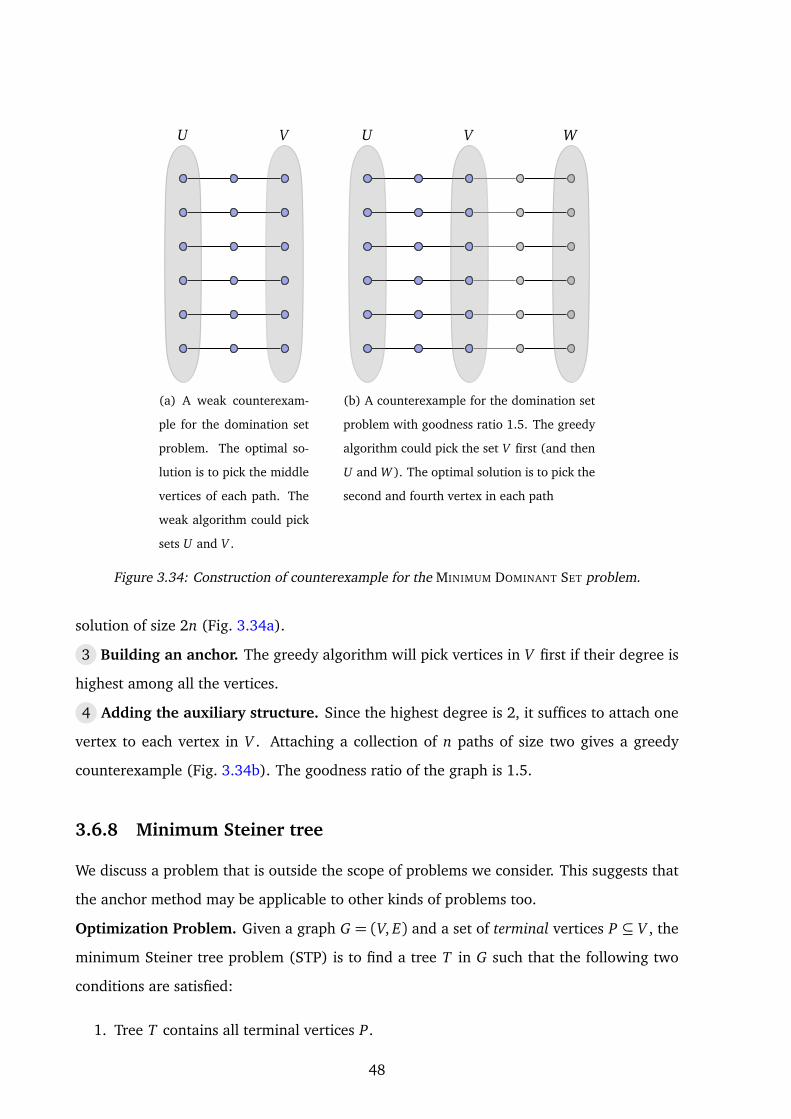
U V
(a) A weak counterexam-
ple for the domination set
problem. The optimal so-
lution is to pick the middle
vertices of each path. The
weak algorithm could pick
sets U and V .
U V W
(b) A counterexample for the domination set
problem with goodness ratio 1.5. The greedy
algorithm could pick the set V first (and then
U and W ). The optimal solution is to pick the
second and fourth vertex in each path
Figure 3.34: Construction of counterexample for the MINIMUM DOMINANT SET problem.
solution of size 2n (Fig. 3.34a).
3 Building an anchor. The greedy algorithm will pick vertices in V first if their degree is
highest among all the vertices.
4 Adding the auxiliary structure. Since the highest degree is 2, it suffices to attach one
vertex to each vertex in V . Attaching a collection of n paths of size two gives a greedy
counterexample (Fig. 3.34b). The goodness ratio of the graph is 1.5.
3.6.8 Minimum Steiner tree
We discuss a problem that is outside the scope of problems we consider. This suggests that
the anchor method may be applicable to other kinds of problems too.
Optimization Problem. Given a graph G = (V, E) and a set of terminal vertices P ⊆ V , the
minimum Steiner tree problem (STP) is to find a tree T in G such that the following two
conditions are satisfied:
1. Tree T contains all terminal vertices P.
48

2. The number of edges in T is minimized.
An example is shown in Fig. 3.35.
a b
de
c
a b
d
c
Figure 3.35: The input graph G with terminals P = a, c, d has a minimum Steiner tree having
three edges. Note that the Steiner tree can contain vertices not in set P.
This problem is not within the scope of our problems since the input is a both a graph
G and a set of vertices (terminals).
Greedy Algorithm. Notice that the Steiner tree must connect all the terminals using the
least number of edges. Since any two terminals must be connected, we try to grow the tree
connecting two vertices along their shortest path.
Definition. For a tree T ∈ G and a vertex v ∈ G, a v T connecting path is the shortest
path that connects vertex v to some vertex in T .
Algorithm 3.6.8: STP(G)
Input: Graph G and a terminal set P
Output: A minimum steiner tree of G
Initially, the tree T contains only the shortest
path amongst all pairs of terminals in the set P.
repeat
1 : Let u be the terminal not in T that
has the shortest connecting path to T .
2 : Add u T connecting path to T .
until the tree T contains
all the terminals in the set P.
Report tree T as the Steiner tree
for the graph G and terminals P.
Constructing a counterexample
49

a b c
d
a b c
d
a b c
d
Figure 3.36: A weak counterexample for the Steiner tree problem. The terminal vertices are a, b
and c. The smallest Steiner tree is the path a− b− c. If the weak algorithm picks the path a− d − c
first, then the Steiner tree will be a− d − c− b which is non-optimal.
1 Weak algorithm. We note that the greedy algorithm starts by picking the shortest path
between all pairs of terminals. We weaken the algorithm slightly by saying the tree could
be initialized with the shortest path between any two terminals.
2 Weak counterexample. Let us try to build a counterexample for the weak algorithm.
The Steiner tree in the graph having two terminals is the shortest path connecting them.
Note that if there are only two terminals the weak algorithm would return the optimal
Steiner tree. It is possible to construct a counterexample having 3 terminals as shown in
Fig 3.36.
3 Building an anchor. The optimal Steiner tree is the path containing 3 terminals. The
weak algorithm could initialize tree T by picking the shortest path between a and c going
via the non-terminal vertex b. This would result in a Steiner tree containing 3 edges. This
serves as our anchor.
4 Adding the auxiliary structure. We can extend the weak counterexample to obtain a
definitive counterexample as shown in Fig. 3.37. The terminal vertices are a, e and c.
a b c
d
e
Figure 3.37: A counterexample with goodness ratio 4/3. The optimal Steiner tree has three edges.
If the greedy algorithm picks the path a − d − c first, then the Steiner tree that is finally obtained
has four edges.
3.7 Pilot Experiment
In order to see which heuristics students apply while constructing counterexamples, we did
a pilot experiment with four students. We will refer them as A, B, C and D. Students A,
50

Pick an easier task
Our approach
Weaken the algorithm
Students’ approaches
Bad first choice
Try small graphs
Reduce from known problem
More general problem
Figure 3.38: Approaches that students tried when constructing counterexamples. The idea of con-
structing a counterexample to a weak algorithm did not occur to any student.
B and C were M.Tech. students who were crediting a course in graduate-level algorithms.
Student D was a Ph.D. student who had secured AA grade in the previous offering of the
same course. All their approaches can be classified into four main categories (Fig.3.38). In
this section, we briefly discuss each category by collating their responses. All the students
were given the following four problems: MAX INDEPENDENT SET, VERTEX COVER, MATCHING
and STEINER TREE.
Force the algorithm to make the wrong choice first. This by far was the most popular
heuristic. All the students were able to construct a counterexample for the vertex cover
problem using this approach (Fig. 3.39). For the MIS problem, most students wrote a star
first and tried to tweak the example such that picking the central vertex leads to a bad
choice (Fig. 3.40). A similar approach was tried for matching problem also. So the only
successful use of this technique was on the vertex cover problem. We observed that students
sometimes failed to acknowledge plausible counterexamples as legitimate counterexamples
and seek to get definitive counterexample directly. For example, for the vertex cover prob-
lem, three out of four students gave a definitive counterexample and only one student gave
a plausible counterexample Fig. 3.39 (b).
Try small graphs. The idea is to check if the algorithm fails for any of the small graphs.
This approach seems natural but is not productive for two reasons. Firstly, even with the
number of nodes not exceeding six, there are many graphs. Unless the student is given a
list of small graphs, as shown in Fig. 3.41, it is time-consuming to enlist all the graphs by
51
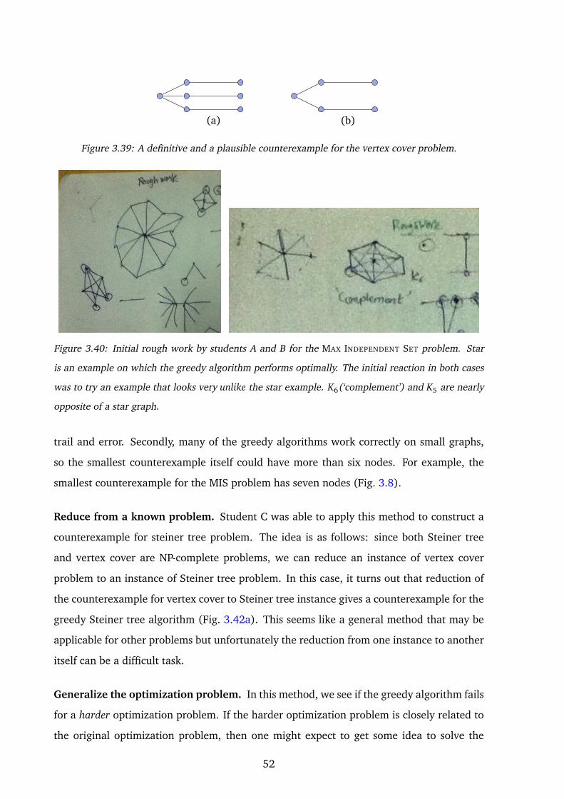
(a) (b)
Figure 3.39: A definitive and a plausible counterexample for the vertex cover problem.
Figure 3.40: Initial rough work by students A and B for the MAX INDEPENDENT SET problem. Star
is an example on which the greedy algorithm performs optimally. The initial reaction in both cases
was to try an example that looks very unlike the star example. K6(‘complement’) and K5 are nearly
opposite of a star graph.
trail and error. Secondly, many of the greedy algorithms work correctly on small graphs,
so the smallest counterexample itself could have more than six nodes. For example, the
smallest counterexample for the MIS problem has seven nodes (Fig. 3.8).
Reduce from a known problem. Student C was able to apply this method to construct a
counterexample for steiner tree problem. The idea is as follows: since both Steiner tree
and vertex cover are NP-complete problems, we can reduce an instance of vertex cover
problem to an instance of Steiner tree problem. In this case, it turns out that reduction of
the counterexample for vertex cover to Steiner tree instance gives a counterexample for the
greedy Steiner tree algorithm (Fig. 3.42a). This seems like a general method that may be
applicable for other problems but unfortunately the reduction from one instance to another
itself can be a difficult task.
Generalize the optimization problem. In this method, we see if the greedy algorithm fails
for a harder optimization problem. If the harder optimization problem is closely related to
the original optimization problem, then one might expect to get some idea to solve the
52

Graph Palette
Path
Cycle
Tree
1 Cycle, 1 Path
1 Cycle, 2 Paths
Small graphs
Figure 3.41: A list of small graphs.
(a) CE by reduction (b) CE by weakening the input
Figure 3.42: Successful application of two different heuristics for the Steiner tree problem.
original problem. For example, instead of building a Steiner tree with unweighted vertices
student D first built a counterexample for the weighted-graph version of the problem and
then converted the counterexample into an unweighted graph (Fig. 3.42b).
The above experiment shows that there are many ways to interpret the phrase ‘solve an
easier problem’ even when we restrict the scope of problems to a small domain. We believe
that the value of anchor method lies in having identified one specific easier problem among
all the available choices.
53

3.8 Discussion
Techniques like greedy, divide-and-conquer, dynamic programming, etc. are quite general
and hence the student does not usually know when a particular method should be applied.
Unlike these techniques, the anchor method is tailor-made for constructing counterexam-
ples for greedy algorithms.
We list some drawbacks of the anchor method:
• Extending the anchor to a counterexample may be hard in some cases. For example,
in the max-leaf problem, it is not obvious that we need to swap a star with a complete
binary tree.
• One may have to try multiple weak counterexamples before hitting upon the right
one that extends to a greedy counterexample.
• Anchor method works only if the weak counterexample gives insight into the structure
of a greedy counterexample. It is ineffective for problems like coin changing[4],
makespan minimization[16], etc. where this is not the case.
In hindsight, the anchor method could have been described directly in terms of ex-
tremal discrepancy graphs. For example, we could have just said:
1. Take a high discrepancy graph and build an anchor.
2. Attach a low discrepancy graph such that the greedy algorithm fails.
The above steps do not use the notion of WISE methodology at all. As we mentioned
in the previous chapter, this is the aspect of WISE that we see in all applications. WISE
scaffolding can be removed once the right extremal graphs are found.
54

Chapter 4
Proving Query Lower Bounds using WISE
4.1 Introduction
The query-model or decision-tree model is a computational model in which the algorithm
has to solve a given problem by making a sequence of queries which have ‘Yes’ or ‘No’
answers. A large class of algorithms can be described on this model and we can also prove
non-trivial lower bounds for many problems on this model. In this chapter, we give a
method to prove lower bounds on the query-model. As in the previous chapter, the method
is a specific application of WISE methodology. In the last chapter, we saw that extremal
graphs with high and low discrepancy played a key role in constructing counterexamples.
Here, we show how certain extremal graphs called critical graphs play a similar role.
Many lower bounds on the query-model are proved using a technique called adversary
argument. In CS courses, a common example used to illustrate the adversary argument is
the following problem: Suppose there is an unweighted graph G with n vertices represented
by an adjacency matrix. We want to test if the graph is connected. How many entries in
the adjacency matrix do we have to probe in order to test if the graph has this property
(property being ‘connectivity’)? Each probe is considered as a query.
Since the adjacency matrix has only n2 entries, O(n2) queries are sufficient. It is also
known that Ω(n2) queries are necessary. Proving this lower bound is more difficult and is
done using the adversary argument.
In literature, we find that lower bound proofs of this problem rely too much on ‘con-
nectivity’ property and do not generalize well. When the property being tested is changed,
the proof changes significantly. Our contribution is a method that gives a systematic way of
55

proving lower bounds for problems involving testing of many graph-properties. We did a
pilot experiment and found that students were able to understand and apply our method.
4.2 Query Complexity
A major focus of computer science is on design and analysis of provably efficient algorithms.
Once we have designed a correct algorithm for a problem, a natural question to ask is: ‘Is
this the best possible algorithm for this problem?’. The only way to know the answer for
certain is to prove that no better algorithm exists. On the Turing-machine computational
model, this question is very difficult to answer and very little is known. So researchers have
been studying the question of proving the optimality of an algorithm on simpler models of
computation. One such model that is widely studied is the ‘query model’ (also known as
decision-tree model).
Query Model. In this model, the algorithm is not given the input directly. The algorithm
has to output the answer by asking queries specified by the problem. The efficiency of the
algorithm is measured by the number of queries it takes in the worst case. The query-model
is popular because a large class of algorithms can be implemented on this model. Hence,
proving optimality of an algorithm on the query model proves its optimality within a large
class of algorithms. For example, consider the problem of sorting n numbers in an array. All
comparison-based algorithms like Quicksort, Mergesort, Heapsort, etc. can be implemented
as query algorithms where a query corresponds to a comparison between a pair of elements
from the array.
Query Complexity. In the query model, we are concerned only with the number of queries
asked by the algorithm and any other computation it may do is irrelevant. The cost of an
algorithm that solves a problem P is the number of queries the algorithm takes in the worst
case to solve P. The cost of an algorithm can usually be expressed as a function of the input
size n. We say algorithm A is better than algorithm B if there exists a constant co such that
the cost of algorithm A is less than B for every problem instance of size n > c0. The query
complexity of a problem P is the cost of the best algorithm that solves P. We denote the
query complexity of the problem of size n by T (n). Query complexity is a property of the
problem and cost is a property of an algorithm.
Given below are four examples of query-model problems. We will refer to all of them
56

later, but our method is applicable only to problems similar to the CONNECTIVITY problem.
Formal descriptions of the first three problems can be found in [6], [3] and [11], respec-
tively.
Problem E1. SORTING. Given an array A of n numbers, sort the elements in the array using
only comparison queries. A comparison query is of the type, ‘Is A[i] smaller or bigger than
A[ j]?’.
Problem E2. ELEMENT DISTINCTNESS. Given an array A of n numbers, find if all the numbers
are distinct, using only comparison and equality queries. An equality query is of the type,
‘Is A[i] equal to A[ j]?’.
Problem E3. 3-SUM. Given an array A of n numbers, find if there exists three numbers in
the array, say a, b and c, such that a + b + c = 0, using only linear-inequality queries. A
linear-inequality query is of the type, ‘Is 3A[1] + 2A[3]− A[6]≥ 0?’.
Problem E4. CONNECTIVITY. Suppose there is a graph G = (V, E) with n vertices. We know
the vertex set V of the graph but not the edge set E. Vertices are labelled from 1 to n. For
any two vertices, a and b with a, b ∈ V , we are allowed to ask the following query: ‘Is (a, b)
an edge in G?’. If G is given by an adjacency matrix, this query is equivalent to probing
the entry at the ath row and bth column of the adjacency matrix of G. What is the query
complexity of determining if the graph is connected?
If the objective of the problem is to determine whether an input satisfies a given prop-
erty or not, then we call such a problem as ‘property-testing’ problem. A property-testing
problem has exactly two possible answers: ‘True’ or ‘False’. For example, problems E2, E3
and E4 are property-testing problems.
Tight lower bounds.1 We call a lower bound tight if it asymptotically matches an up-
per bound of T (n). We are interested in obtaining tight asymptotic bounds on T (n) for
problems involving testing of graph-properties (similar to Prob. E4).
Overview of techniques. There are four main techniques for proving query lower bounds.
The four problems E1-E4 are generally used as examples to illustrate each technique (Sec. 4.3).
However, our focus is only on proving lower bounds for testing graph properties. The
known methods for proving lower bounds for this kind of problems are ad-hoc in nature
and rely on problem-specific observations. Our main contribution is a method that gives a
1Most of the terminology we use is standard. Definitions of algorithmic terms and graph theoretic terms
can be found in [21] and [34], respectively.
57

more systematic way of proving lower bounds (Sec. 4.7). In Sec. 4.8, we show that our ap-
proach works for many problems within the scope. We did a pilot experiment and observed
that students are able to understand and apply our method (Sec. 4.9).
4.3 Related Work
We review known methods for proving query lower bounds and provide context for our
work.
Information-theoretic proof. An explanation of this method can be found in Chap-
ter 8 of [6]. The main assertion of the proof is the following:
Fact. If a problem P has M possible outputs and the input to the problem can be
accessed only via ‘Yes/No’ queries, then log2 M is a query lower bound for P.
In other words, log2 M is the minimum number of queries any correct algorithm
must ask, in the worst case. For example, in the sorting problem, if the input consists
of n numbers, then there are n! possible outputs. Each output corresponds to a differ-
ent ordering of n numbers. So we can claim that the lower bound for sorting problem is
log2 n!= Ω(n log n).
However, this method is not useful for property-testing problems. In a property-testing
problem, there are only two outputs: ‘True’ or ‘False’. The information-theoretic proof only
gives a trivial lower bound of one (log2 2= 1).
Algebraic Methods. In 1983, Ben-Or gave an algebraic technique that proves a tight
Ω(n log n) lower bound for ELEMENT-DISTINCTNESS problem. His technique, in one stroke,
proves non-trivial lower bounds for twelve different problems [3]. But problems E3 and E4
are not amenable to this technique.
Reduction. Reduction is another way of proving lower bounds. At undergraduate-
level, reduction is often taught in the context of NP-hardness. If we want to show that
problem H is NP-hard, we do so by proving that some known NP-hard problem (like SAT)
reduces to H in polynomial time. Query lower bounds can also be proved in a similar
vein. Suppose we know that a problem R has query complexity of Ω(g(n)) on a certain
computation model, we can show that another problem S has query complexity Ω(g(n)) on
the same model by reducing problem R to S in o(g(n)) time. For example, we know that
finding the convex hull of a set of n points takes Ω(n log n) operations because the sorting
58
problem reduces to it (Prob. 33.3-2 in [6]).
The 3-SUM problem is known to have a query complexity of Θ(n2) [11]. The lower
bound proof of 3-SUM does not result in any general technique. But the strength of 3-SUM
lies in the fact that this problem is an excellent candidate problem for proving lower bounds
by reductions. Several problems in computational geometry have been shown to be as hard
as 3-SUM [12]. But a lower bound for Prob. E4 cannot be proved by reduction either.
Adversary Arguments. What can we do if none of the above three methods work?
We take recourse to proving by ‘first principles’, commonly known as proving by adversary
argument. Recall that a lower bound of g(n) for a problem P means that any correct algo-
rithm must make at least g(n) queries to solve P. So if we show that any algorithm that
makes strictly less than g(n) queries must be incorrect, then we have proved a lower bound
of Ω(g(n)) for the problem. Imagine that the queries asked by the algorithm are answered
by an adversary. The adversary’s objective is to maximize the number of queries that the
algorithm asks and the algorithm’s objective is to minimize the number of queries. If an
adversary can force any correct algorithm to ask at least g(n) queries, then g(n) is a lower
bound on the query complexity of the problem. It is necessary to understand the format of
adversary arguments in order to follow the proofs in this paper. Introduction to adversary
method can be found in [10] or [29]. Two proofs that give exact lower bounds for Prob. E4
can be found in [10] and [2]. Both the proofs are based on adversary arguments. However,
these proofs do not generalize easily to other graph properties. In the next section, we give
a different proof for this problem using an adversary argument. Though our proof gives
only an asymptotic tight lower bound, it generalizes easily to other graph properties.
4.4 Adversary Argument Revisited
Terminology
Notation. Throughout the chapter, the notation G = (V, E) refers to an undirected un-
weighted graph G with n vertices, where V is the vertex set and E is the edge set. We may
assume that the vertices are labeled from 1 to n. We denote a complete graph having r
vertices by Kr .
Definition. If there is no edge present between a pair of vertices u and v in a graph, we say
59

(u, v) is a non-edge in the graph.
4.4.1 Testing Connectivity
Problem E4. We are given access to a graph G = (V, E) via queries of the form ‘Is (a, b)
an edge in G?’. We know the vertex set V but not the edge set. Prove that it takes at least
Ω(n2) queries in the worst case to determine if G is connected.
Proof: We prove that any correct algorithm must take at least n2/4 queries. For contra-
diction’s sake, let us assume that there is a correct algorithm A that makes less than n2/4
queries. We first describe the adversary’s strategy for answering queries asked by the algo-
rithm and then give the analysis.
Let G1 be the graph made of two complete subgraphs A and B, such that A has nodes
labelled from 1 to n/2 and B has nodes labelled from n/2+ 1 to n (Fig. 4.1 (a)). Note that
graph G1 has the same vertex set V as G.
Adversary’s Strategy. The adversary first picks the graph G1 tentatively as input (in
its mind) and answers the queries posed by the algorithm as follows:
When the algorithm asks ‘Is (a, b) an edge in G?’, the adversary says ‘Yes’ if
(a, b) is an edge in G1 and ‘No’ if (a, b) is a non-edge in G1.
The adversary also keeps track of all the queries asked by the algorithm.
Analysis. Consider the moment when all the queries are made and A has declared
whether G is connected or not. By our assumption, A has made less than n2/4 queries.
Since there are n2/4 non-edges in G1, there exists some pair of vertices (say (i, j)) such
that:
• Pair (i, j) is a non-edge in G1.
• A did not ask the query ‘Is (i, j) an edge in G?’
Let G2 be the graph obtained by replacing the non-edge (i, j) in G1 by an edge (Fig. 4.1 (b)).
G1 is not connected but G2 is connected. But both the graphs are consistent with all the
answers the adversary has given. The adversary can prove that algorithm A is wrong as
follows:
60

If the algorithm outputs ‘True. G is connected’, the adversary ‘reveals’ that G = G1 and
shows that the algorithm is wrong. If the algorithm outputs ‘False. G is not connected’, the
adversary reveals that G = G2 and again proves the algorithm wrong.
So regardless of what the algorithm outputs, the adversary can always contradict the
algorithm. Hence, every correct algorithm must make at least n2/4 queries.
Kn/2
A
Kn/2
B(a) G1
Kn/2
A
Kn/2
Bi j
(b) G2
Figure 4.1: (a) G1 is the graph the adversary tentatively keeps as input in its mind. Every pair of
vertices (p, q) with p ∈ A and q ∈ B in a non-edge in G1. So G1 has n2/4 non-edges. (b) G2 is the
graph obtained by replacing the non-edge (i, j) in G1 with an edge. G2 is connected but G1 is not.
Since (i, j) was not queried by the algorithm, both G1 and G2 could have been possible inputs to the
problem.
4.5 Scope of Problems
Our method is applicable to problems of the following kind.
GENERIC-PROBLEM. There is a graph G = (V, E) to which we do not have direct access.
We know the vertex set but not the edge set. There are n vertices in G and we may assume
that they are labelled from 1 to n. We are allowed to ask queries of the type ‘Is (a, b) an
edge in the graph G?’, where a, b ∈ V . The problem is to find if G has a given property P
by asking such queries.
4.5.1 Our approach
In order to prove a lower bound for the GENERIC-PROBLEM, when property P is specified
explicitly, we do the following:
• Construct a critical graph G for property P which has many non-edges. We will define
a critical graph shortly.
61

• Apply Theorem 4.7.1 which says that existence of a critical graph with many non-
edges implies a lower bound for the problem.
4.6 Query lower bounds using WISE
We describe how the key idea in the lower bound proof of connectivity was obtained using
WISE.
Weakened Problem. In the proof of connectivity we have weakened the problem in
two ways:
• Firstly, the possible inputs is resctricted to only those graphs which have at most two
connected components.
• Secondly, we seek to obtain only an asymptotic bound although an exact bound is
possible. We shall see that this trade-off helps in proving lower bounds for other
graph properties.
Identifying a candidate problem. Even after restricting the input graphs to at most
two connected components there are a few choices (Fig 4.2). We choose to identify the
case where the graph is composed of two complete graphs (Fig 4.2(b)) for the purpose of
proving the lower bound.
(a)
Kn/2 Kn/2
(b) (c)
Figure 4.2: Graph (a) is extremal because the discrepancy between the size of two connected com-
ponents is maximum. Graphs (b) and (c) are graphs in which the discrepancy between the sizes in
minimum. Graph (b) has maximum number of edges within each component (Kn/2) while graph
(c) has the minimum number of edges needed for connectivity (n/2− 1).
Solving the candidate problem. We prove a lower bound of n2/4 using the adversary
arguement (Sec. 4.4).
Extending the solution. However, we can extend the solution to prove lower bounds
for other properties. In the next section, we show how the proof of connectivity lower
62

bound can be extended to solve the generic problem given in Sec. 4.5. Unfortunately, it is
not possible to extend the solution to get an exact query lower bound, so all the bounds are
still asymptotic.
4.7 Main Theorem
Definition. Given a property P, a graph Gc is said to be critical with respect to the property
if the following two conditions are met.
(C1) Gc does not have the property P.
(C2) Replacing any non-edge in Gc by an edge endows the graph with property P.
For example, if the property is ‘Connectivity’, then the graph shown in Fig. 4.1 (a) is
an example of a critical graph.
We will now prove our main result using ideas very similar to the proof of CONNECTIV-
ITY problem (Sec. 4.4.1).
Theorem 4.7.1. Suppose Gc is a critical graph for the property P. If Gc has n vertices and
x non-edges, then x is a query lower bound for the GENERIC-PROBLEM.
Proof: We show that any correct algorithm must make at least x queries in the worst case.
We prove by contradiction. Assume that there is some algorithm A that solves the GENERIC-
PROBLEM by making strictly less than x queries.
We first give an adversary’s strategy for answering queries by A and then give the
analysis.
Adversary’s Strategy. The adversary first constructs the graph Gc (in its mind) and
answers the queries posed by the algorithm as follows: When the algorithm asks ‘Is
(a, b) an edge in G?’, the adversary says ‘Yes’ if (a, b) is an edge in Gc and ‘No’ if (a, b) is a
non-edge in Gc.
Analysis. Consider the moment when all the queries are made and A has declared
whether G has the property P or not. By our assumption, A has made less than x queries.
Since there are x non-edges in Gc, there exists some pair of vertices (say (i, j)) such that:
• Pair (i, j) is a non-edge in Gc.
• A did not ask the query ‘Is (i, j) an edge in G?’
63

By our definition of critical graph, we have the following:
• Graph Gc does not have property P.
• Suppose G′c is a graph which is the same as Gc except that the non-edge (i, j) in
Gc is replaced by an edge in G′c. So G′c has exactly one more edge than Gc. More
importantly, G′c has the property P, since Gc was a critical graph.
Either Gc or G′c could have been the input graph for the problem since they are con-
sistent with all the answers the adversary has given. But one graph has the property and
the other one does not. Hence, whatever answer the algorithm outputs, the adversary can
prove the algorithm wrong. Hence, any algorithm that makes less than x queries must be
incorrect.
Now we turn to the applications of this theorem.
4.8 Applications
We prove lower bounds for many common graph properties by constructing a critical graph
for each property. It turns out that all the problems we consider have a lower bound of
Ω(n2), which proves that the bounds are asymptotically tight.
For each problem, we describe how to construct a critical graph with Ω(n2) number of
non-edges. The lower bound follows from Theorem 4.7.1.
We will use the following handy fact repeatedly.
Lemma 4.8.1. A graph with n vertices and m edgesn
2
−m non-edges.
Proof: There aren
2
pairs of vertices in a graph. Between every pair of vertices, either
there is an edge or a non-edge.
4.8.1 Triangle Detection
A graph G is said to have a triangle if K3 is a subgraph of G.
Problem P1. Given access to G = (V, E) via queries of the form ‘Is (a, b) an edge in
G?’ determine if G has a triangle.
64

Construction of Gc. A rooted star tree with the root node as 1 (Fig.4.3). In other words,
Gc is a graph where we connect node 1 to every other node. There are exactly n− 1 edges
in Gc.
It is easy to verify that Gc satisfies both the conditions of a critical graph.
(C1) Gc does not have triangle.
(C2) Replacing any non-edge in Gc, induces a triangle involving node 1.
No. of non-edges in Gc:n
2
− (n− 1) = Ω(n2).
By Theorem 4.7.1, any algorithm must make at least Ω(n2) queries. Since this step
is same for all problems, in subsequent examples, we only describe the construction of the
critical graph.
. . .
1
2 3 n
Figure 4.3: A critical graph for ‘has a triangle’ property. Node 1 is connected to every other node.
The non-edges are between nodes 2, ...n.
4.8.2 Hamiltonian Path
Problem P3. Given access to a graph G = (V, E) via queries of the form ‘Is (a, b) an edge in
G?’ determine if G has a Hamiltonian path.
Construction of Gc. We build two complete subgraphs A and B of equal size such that A
has nodes labelled from 1 to n/2 and B has nodes labelled from n/2+ 1 to n (Fig. 4.4).
Kn/2
A
Kn/2
B(a)
Kn/2
A
Kn/2
B(b)
Figure 4.4: (a) A critical graph Gc for Hamiltonian property. Gc does not have a Hamiltonian path
since it is disconnected. (b) Replacing any non-edge by an edge induces a Hamiltonian path.
65

4.8.3 Perfect Matching
Problem P3. A graph G is said to have a perfect matching if there exists a pairing of all
nodes in G, such that every node is contained in exactly one pair and each pair has an edge
between them. A necessary (but not sufficient) condition for G to have a perfect matching
is that n must be an even number. Given access to G = (V, E) via queries of the form ‘Is
(a, b) an edge in G?’ determine if G has a perfect matching. Assume that n is even.
Construction of Gc. Since n is an even number, assume that n = 2s. If s is an odd number,
we construct two complete subgraphs A and B such that A has nodes from the set 1, .., s
and B has nodes from the set s+1, .., n. If s is an even number, we construct two complete
graphs A and B such that A has nodes in the set 1, .., s−1 and B has nodes in the set s, .., n
(Fig. 4.5). Basically, we want to ensure that both A and B have odd number of nodes.
We show that Gc satisfies both the conditions of a critical graph.
(C1) Gc does not a perfect matching. This is because both A and B have odd number of
vertices and hence one vertex in A and B will always be unmatched.
(C2) Replacing any non-edge (a, b) in Gc, induces a perfect matching. We pick the edge
(a, b) in the matching and remove it from Gc. Now both A and B have even number of
unmatched vertices, hence we can find a perfect matching.
No. of non-edges is s2, when s is odd and s2 − 1 when s is even. Hence, number of
non-edges x ≈ n2/4.
Ks−1
A
Ks+1
B(a)
Ks−1
A
Ks+1
B(b)
Figure 4.5: (a) Critical graph Gc for ‘perfect matching’ property when s is even. Graph Gc does not
have a perfect matching since A and B have odd number of vertices. (b) If we replace any non-edge
by a edge then it is easy to verify that the graph obtained has a perfect matching.
4.8.4 Non-Bipartite Detection
Problem P4. Given access to G = (V, E) via queries of the form ‘Is (a, b) an edge in G?’
determine if G is non-bipartite.
66
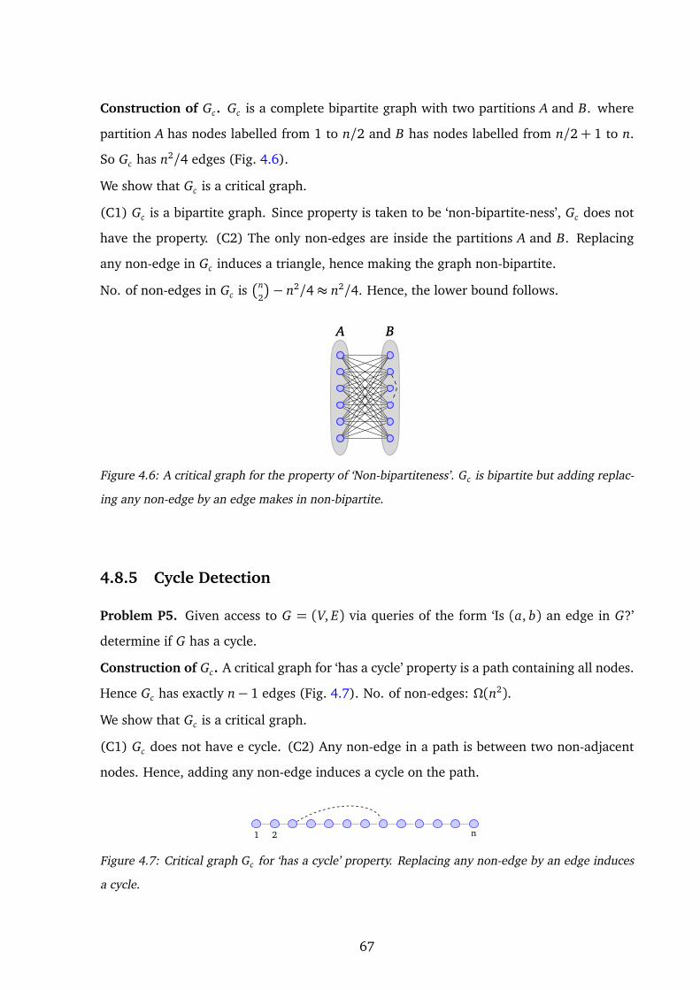
Construction of Gc. Gc is a complete bipartite graph with two partitions A and B. where
partition A has nodes labelled from 1 to n/2 and B has nodes labelled from n/2+ 1 to n.
So Gc has n2/4 edges (Fig. 4.6).
We show that Gc is a critical graph.
(C1) Gc is a bipartite graph. Since property is taken to be ‘non-bipartite-ness’, Gc does not
have the property. (C2) The only non-edges are inside the partitions A and B. Replacing
any non-edge in Gc induces a triangle, hence making the graph non-bipartite.
No. of non-edges in Gc isn
2
− n2/4≈ n2/4. Hence, the lower bound follows.
A BA B
Figure 4.6: A critical graph for the property of ‘Non-bipartiteness’. Gc is bipartite but adding replac-
ing any non-edge by an edge makes in non-bipartite.
4.8.5 Cycle Detection
Problem P5. Given access to G = (V, E) via queries of the form ‘Is (a, b) an edge in G?’
determine if G has a cycle.
Construction of Gc. A critical graph for ‘has a cycle’ property is a path containing all nodes.
Hence Gc has exactly n− 1 edges (Fig. 4.7). No. of non-edges: Ω(n2).
We show that Gc is a critical graph.
(C1) Gc does not have e cycle. (C2) Any non-edge in a path is between two non-adjacent
nodes. Hence, adding any non-edge induces a cycle on the path.
1 2 n
Figure 4.7: Critical graph Gc for ‘has a cycle’ property. Replacing any non-edge by an edge induces
a cycle.
67

4.8.6 Degree-Three node
Problem P6. Given access to G = (V, E) via queries of the form ‘Is (a, b) an edge in G?’
determine if G has a node whose degree is three.
Construction of Gc. A critical graph for property ‘has a degree-3 node’ is a cycle containing
all the nodes. Every node has degree exactly two. Adding any non-edge would make some
vertex have degree three (Fig. 4.8). Since Gc has exactly n edges, the number of non-edges
is Omega(n2).
1
2
3
4
5
6. . .
n
Figure 4.8: Critical graph Gc for ‘has a degree-3 node’ property. Gc has all nodes of degree two so
replacing any non-edge by an edge gives a degree-3 node.
4.8.7 Planarity
Problem. Given an access to graph G = (V, E) via queries of the form ‘Is (a, b) an edge in
G?’ determine if G is a planar graph.
Solution.
The construction of property-critical graph for planarity is a bit tricky since it requires
some known facts about planar graphs. A planar graph G is said to be triangulated if
the addition of any edge to G results in a non planar graph. For example, a triangulated
graph for n = 6 is shown in Fig. 4.9. So by our definition any triangulated planar graph
is property-critical. It is a well-known fact in graph theory that any triangulated planar
graph has exactly 3n− 6 edges. This means the number of non-edges isn
2
− (3n− 6) =
(n2− 7n+ 12)/2. Hence, the query lower bound for planarity testing is Ω(n2).
68

Figure 4.9: A triangulated graph having six vertices. This is a property-critical graph for planarity
for n= 6. There are exactly 3n− 6= 12 edges in the graph.
4.9 Teachability
We did a pilot experiment with five CS graduate students to see if they could apply our
method to derive query lower bounds. We report our findings in this section.
Design. The author had one-on-one interview-type session with each student. Prior
to the start of the session, we made sure that the student understood the basic concepts
and definitions related to query computational model. A session lasted for 2-4 hours and
was divided into three phases. In the first phase, the students understood the format of
adversary arguments. In the second phase, the student attempted to solve the CONNECTIVITY
problem (Prob. E4) for one hour. Our objective was to allow the students to try the problem
on their own so that we could identify the common approaches taken to solve the problem.
The student was encouraged to think aloud during this time. If he persisted in a wrong
approach for more than ten minutes, the author alerted the student to the mistake and let
him continue. At the end of one hour, regardless of how the student performed, the author
gave the solution to the problem along with an explanation of the method as described in
Sections 4.4-4.7. The student was also given the solution given in [2]. In the third phase,
the student attempted to derive lower bounds for the list of problems given in Sec. 4.8,
without any help. We describe observations made in each phase below.
4.9.1 Phase I: Adversary Argument Explained
In the first phase, the students got familiar with the adversary argument. Two students who
said they were familiar with adversary arguments were quizzed on the topic with a couple of
questions. The other three students found it easy to follow the adversary argument through
examples like ‘n-Card Monte’ and ‘20-questions’, given in [10] and [29], respectively. Some
students took more time than others to understand the format of the proof, which accounted
69

for the variability in the duration the sessions.
4.9.2 Phase II: Teaching
We list common failed approaches taken while solving the CONNECTIVITY problem.
Failed approach F1. Students find it hard to let go of the algorithm and think like an
adversary. They often prove lower bounds assuming that the algorithm works in a certain
way. For example, four out of five students gave the answer along the following lines:
“Every vertex has n− 1 possible incident edges. When the algorithm asks n− 1 queries for
a vertex, the adversary answers with a ‘Yes’ only for the last incident edge.” The flaw in this
reasoning is the assumption made about the algorithm’s behavior. The algorithm need not
ask queries in an orderly manner. The lower bound has to work for any algorithm, not just
the one that probes vertex-by-vertex.
Failed approach F2. All the students tried for exact bounds which is harder than proving
asymptotic bounds. Even when the students were reminded that only asymptotic lower
bound is sufficient, they could not figure out a way to make use of the relaxed constraint.
Failed approach F3. Three students came up with the correct adversary strategy, but failed to
do the analysis. The strategy was: The adversary always says ‘No’ unless saying so definitely
disconnects the graph. This strategy is intuitive and is also correct, but unfortunately none
of them were not able to prove that it works. The correct analysis of this strategy is given
in [2].
4.9.3 Phase III: Testing
In Table 4.1, we give the time taken by each student to construct the correct critical graph.
Some students gave different (correct) critical graphs than the ones we have given. For
example, for ‘Triangle’ property two students gave complete bipartite graph as the answer.
Similarly, for ‘Cycle’ property all the students gave ‘any spanning tree’ as the answer. As it
can be seen from Table 4.1, most students were able to construct critical graphs quickly. We
observed that three students who were not familiar with adversary arguments did equally
well as the other two students. We did not anticipate this but it seems reasonable in hind-
sight. After all, the main reason why our method is helpful is because it shifts the focus
from designing an adversary strategy to finding one critical graph. So prior knowledge of
70

adversary arguments did not matter as much.
Inference. Although the textbook-proof was known to the students, all of the them chose to
prove using critical graphs. This shows that the students found our method easier to apply.
In the words of a student, “Instead of thinking about how the queries must be answered,
I just have to look for the right graph, which seems easier to do”. We also asked students
S1 and S5 to attempt solving the problems without using critical graphs. Student S1 was
able solve problems P1 and P5 and student S5 was able to solve P1 and P4. Both of them
could not solve the other problems in a time duration of 15 mins (per problem). This too
suggests that the textbook-proof is not easily applicable to other graph properties.
Phase Topic Students
S1 S2 S3 S4 S5
I Adv. Yes Yes No No No
II E4 F2 F1,2,3 F1,2 F1,2,3 F1,2,3
III
P1 8m 10m - 9m -
P2 5m 5m 9m 6m 6m
P3 8m - - 10m 9m
P4 1m 2m 4m 2m 2m
P5 1m 2m 2m 1m 2m
P6 1m 1m 1m 1m 1m
Table 4.1: Summary of data from the experiment. Phase I: ‘Yes’ means that the student already knew
the adversary method. Phase II: Subscripts in F refer to the failed approaches taken by the student
as discussed in Sec. 4.9.2. Phase III: Numbers give the time taken by the student to answer. A -
against a problem means that the student was not able to answer that problem within 15 minutes.
The time taken is shown in minutes.
71

4.10 Discussion
WISE methodology was used only to solve the connectivity problem. Once we obtain the
insight about critical graphs, we discard the WISE scaffold and solve problems purely using
extremal critical graphs. Again, this points to the invisibility of WISE. In the next chapter
on tree learning, we see that this aspect is even more pronounced.
Remark. An alternate approach to proving lower bounds for graph-properties can be found
in [20]. However, this proof method is beyond the scope of most CS courses since it relies
on deep ideas in topology.
Remark. There is a lacuna in most traditional textbooks when discussing lower bounds.
But lower bounds as a topic in complexity theory has gained a lot of importance in the last
few years. In support of this claim, we would like to point out that the recent book by Arora
and Barak titled ‘Computational Complexity: A Modern Approach’ [2] has one-third of the
book devoted exclusively to lower bounds.
72

Chapter 5
Tree Learning Algorithm using WISE
In the previous chapters, we used the WISE methodology to derive solutions to only text-
book problems. But the methodology is powerful enough to solve even a research problem.
We describe the problem and give an account of how the key ideas of the algorithm were
derived using WISE.
Problem Definition. Suppose T is an undirected binary tree containing n nodes. We know
the nodes in T but not the edges. The problem is to output the tree T by asking queries of
the form: “Does the node y lie on the path between node x and node z?”. In other words,
we can ask if removing node y disconnects node x from node z. Such a query is called a
separator query. Assume that each query can be answered in constant time by an oracle.
The objective is to minimize the time taken to output the tree in terms of n.
Role of WISE. By designing algorithms for certain extremal input instances we can get a
sub-quadratic algorithm. We weaken the problem by restricting the input instances to these
three graphs: path, complete binary tree and centipede. For each extremal instance, we get
an algorithm and extend it to more a general case (Table 5.1). Putting all the ideas together
gives an O(n1.8 log n) algorithm.
Remark. The problem is motivated by an application in machine learning. The details
of the motivation can be found in [26]. Also, [26] contains an improved algorithm that
runs in O(n1.5 log n) time. WISE methodology is useful only to the extent of obtaining
an O(n1.8 log n) algorithm. This is interesting since no sub-quadratic time algorithm was
known prior to our work. The result is joint work with Anindya Sen.
In Section 5.0.1 we discuss some preliminaries. In Section 5.0.2 we give a naïve O(n2)
algorithm. We then discuss the main result where we use WISE to derive a sub-quadratic
73

algorithm for the problem.
5.0.1 Preliminaries
Notation. Let V (T ) refer to the node set of T and E(T ) to the edge set of T . Note that
n = |V (T )|. Let x y z denote the separator query “Does node y lie on the path
between node x and node z?”. We call y as the middle node in the query x y z.
Lemma 5.0.1. Let x and z be a pair of nodes in tree T . The set of all nodes that lie on the
path between x and z can be found in O(n) time using the separator queries.
Proof: A node i lies on the path between x and z only if x i z is true. This requires
n− 2 calls to the oracle.
Lemma 5.0.2. Let x and z be a pair of nodes in the tree T . The path P between node x
and node z can be found in O(n log n) time using the separator queries.
Proof: Using Lemma 5.0.1, we find the set of nodes that lie on the path P. We then impose
a total order on the nodes on the path as follows: for any pair of nodes yi and y j belonging
to P, node yi is greater (resp. smaller) than y j if x yi y j is true (resp. false). Finally,
the path is obtained by ‘sorting’ the nodes according to the total order defined above.
Lemma 5.0.3. Suppose we know that (p, q) is an edge in tree T . Let T1 and T2 be the two
subtrees that result from removing the edge (p, q). We can find the set of nodes that belong
to T1 and T2 in O(n) time.
Proof: Every node i must lie on either side of the edge (p, q). If i p q is true, node i
belongs to T1 and if p q i is true, it belongs to T2.
In the rest of the chapter, we assume that separator queries can be answered in con-
stant time and avoid explicit references to the oracle when describing algorithms.
5.0.2 A naïve O(n2) algorithm
We give an algorithm that learns the structure of a tree in O(n2) time. The result applies to
unbounded degree trees also.
74

Lemma 5.0.4. The neighbors of any given node v with degree d(v) can be found in O(d(v)n)
time.
Proof: The procedure to find a neighbor is similar to finding the minimum element in a
given set of numbers. Suppose we want to find a neighbor of a node v. Initialize a variable
min to an arbitrary node other than v (say vx). Let vv1v2v3 . . . vx be the path from v to vx .
Suppose v u min is true for some node u, then it means that
• Node u is some vi.
• Node vi is closer to v than min. In other words, distance from node v to vi is lesser
than the distance from node v to min.
Iterate through every node i updating min to i if v i min is true. In the end,
min will contain v1. We found one neighbor of v in O(n) time. To find another neigh-
bor of v, throw away the newly-discovered neighbor v1 and the set of nodes S = x :
v v1 x is true and repeat the above procedure. We keep repeating this step until all
the neighboring nodes of v are discovered. Since v has degree d(v), it takes O(d(v)n) time
to discover all the neighbors of v.
We can find the neighbors of every node using the above procedure and learn the
structure of the tree. Since the sum of degrees of all the nodes in the tree is 2(n− 1), the
above algorithm takes O(n2) time.
A sub-quadratic algorithm using WISE. We solve the problem for a few extremal input
instances and then use the key ideas to obtain a better algorithm for the tree learning
problem. The presentation style is as follows. We restrict the input to an extremal instance,
discuss the algorithm specific to that instance and then extend the idea to cover a more
general case. The extremal input instances and their generalizations are given in Table 5.1.
5.1 Iteration 1: From path to bounded leaves tree
Step 1-1 Analyze the problem
Instances of the problem: Tree. Properties of trees: Number of leaves, maximum degree of
vertex, diameter, etc. Extremal cases: Paths and complete binary trees.
75

Iteration Extremal Input Generalization
1. Path Bounded leaves tree
2. Complete binary tree Short-diameter tree
3. Centipede Long diameter trees
Table 5.1: The algorithms designed for the extremal trees extend to more general input cases.
Step 2-1 Weakening
We weaken the instance of the problem to an extremal case: consider the simplest instance
when the tree is a path.
Step 3-1 Candidate problem 1: Path
We show how to solve the problem if T is restricted to a path.
Step 4-1 Solution
We can impose a total ordering among the nodes of a path as follows. Let x be a leaf node
in the path. Node a is greater (resp. lesser) than b if x a b is true (resp. false). Hence,
learning the structure of a path is equivalent to sorting n numbers on a comparison model.
We use the separator query like a comparison operator and get an O(n log n) algorithm.
Step 5-1 Generalization 1: Bounded leaves
Intuition. Consider the near-extremal case when the tree is a union of two paths. In this
case, we can first collect all the nodes that lie on one path. Learn one leaf-to-leaf path and
then learn the remaining path next. So if the tree had three leaves as shown below, then
the time taken to learn the tree is still O(n log n).
76

We can generalize this idea to the case when the tree has l leaves.
Sol.
Lemma 5.1.1. The tree with n nodes and l leaves can be learnt in O(nl log n) time using
the oracle.
Proof: Select an arbitrary node r as the root node. Initialize a variable f to a node other
than r. If r f u is true for some node u, then it means that node u is farther to r than
f . Iterate through every node i updating f to i if r f i is true. In the end, f will
contain some leaf. We find all the nodes on the path from r to f . In this way we can learn
a root-to-leaf path in O(n log n) time. Since the tree has only l leaves it takes O(nl log n)
time to learn the tree.
5.2 Iteration 2: From binary tree to short diameter
Step 1-2 Add a difficulty
Lemma 5.1.1 implies a sub-quadratic algorithm for the tree learning problem if the number
of leaves is o(n). So we consider the bad case when the number of leaves is O(n).
Step 2-2 Weakening
Which extremal structure has O(n) leaves? The complete binary tree serves the purpose
since it has n/2 leaves.
Step 3-2 Candidate problem 2: Complete binary tree
We solve the problem for the case when T is a complete binary tree.
Step 4-2 Solution to binary tree
Intuition. If we could find the root node we can recurse on the subtrees. Suppose we pick
a node (say 11 in Fig. 5.1) and learn its neighbours. We can move towards the root node
by going in the direction which contains the largest number of nodes. For example, since
77

6
13
11
5 8
10
9 2
15
12
1 3
14
4 7
Figure 5.1: At each step, we can get closer to the root by moving in the direction of the larger
number of nodes
we have picked 11 we find its neighbours are 5, 8 and 13. Out of these neighbours the
maximum number of nodes lie in the direction of node 13, therefore node 13 is closer to
the root node.
Sol. We give an algorithm that runs in O(n log2 n) time. The idea is to pick a vertex and
get closer to the root.
We find the root node as follows:
1. Pick any vertex a.
2. Find the neighbours of the vertex a (say x , y and z).
3. If vertex a has exactly two neighbours, then we have found the root. Otherwise,
count the number of vertices that remain connected to x if edge (a, x) is removed.
Call this number C(x). Similarly find C(y) and C(z).
The vertex i with maximum C(i) is closer to the root than vertex a, so repeat the
above steps with vertex i.
Analysis. All the three steps can be done in O(n) time. We may have to move up log n
times, so it takes O(n log n) time to find the root node.
Once we find the root we recurse on the sub-trees, so overall it takes O(n log2 n) to
learn the tree.
Step 5-2 Generalization 2: Short diameter
We now generalize the above idea to trees with diameter D.
We state a folklore lemma that gives the analogue of a root node of a complete binary
tree. An edge is called an even separator if its removal splits the tree into two trees each of
whose size is between 2n/3 and n/3.
78

Lemma 5.2.1. Every binary tree T has an even separator.
Proof: We give a constructive proof. Orient every edge in T in the direction of the larger
number of nodes, breaking ties arbitrarily. If T has more than two nodes, then all the
leaves will have in-degree zero and out-degree one. Since the number of nodes in T are
fixed, any maximal directed path in T must end at some vertex m whose out-degree is
zero. Since m cannot be a leaf it has either two or three edges incident on it. We show
that one of the incident edges is an even separator. Root the tree at m. Let x , y and z
be the children of m. Let C(x), C(y), C(z) be the number of nodes sub-rooted at x , y and
z, respectively. Without loss of generality assume that C(x) ≤ C(y) ≤ C(z). The relations
C(x)+C(y)+C(z) = n−1 and C(x)+C(y)≥ C(z) ensure that C(z) ∈ [n/2, 2n/3]. Hence,
edge (m, z) is an even separator.
Claim 5.2.2. A constant-degree tree with diameter D can be learnt in O(nD log n) time.
Proof: Here is an algorithm to learn the tree:
1. Pick any edge e with endpoints p and q.
2. Check if e is an even separator. This can be done by counting the number of nodes
that lie on either side of e.
3. If e is an even separator, label p and q and recurse on the subtrees rooted at p and q.
4. If e is not an even separator, move to a neighboring edge that lies in the direction
of the larger number of nodes and which gives a better split. For example, if p is in
the direction of the larger number of nodes then we check the other neighbours of
p and move to the edge that gives a better split. We get one step closer to the even
separator by doing this. Repeat Step. 2-4.
Since the diameter of the tree is D, it takes at most D steps to find the even separator. Each
step takes O(n) time. Once we get the separator, we divide and recurse on the subtrees.
Hence, we can learn the tree in O(nD log n) time.
The above idea can be generalized to give a sub-quadratic algorithm whenever the
diameter of the tree is o(n). The hard-case is when the tree has a long diameter.
79

5.3 Iteration 3: From centipede to long diameter tree
Step 1-3 Add a difficulty
Now we know that if the tree has either small diameter or bounded leaves a sub-quadratic
time algorithm is possible. So the hard case is the class of trees which have Ω(n) diameter
and Ω(n) leaves.
Step 2-3 Weakening
We want an extremal graph that has a long diameter and a lot of leaves. A centipede serves
the purpose. A centipede is a tree which has a diameter of length n/2 and has n/2 leaves.
Step 3-3 Candidate problem 3: Centipede
How quickly can we learn if the tree is a centipede?
Sol. We describe an O(n log n) algorithm to learn a centipede.
Definition. A bead is a vertex with more than degree one and a leaf is a vertex with
degree one. A centipede has equal number of beads and leaves. The key idea in the
algorithm is to get one bead in constant time on an average.
Lemma 5.3.1. If a x b returns ‘Yes’ then the middle node x has to be a bead.
Proof: The centipede has only leafs and beads. A leaf cannot appear on a path between
two nodes.
Claim 5.3.2. Suppose S is a set of nodes that lie on the right side of a bead r. If S has x
beads, we can find at least x − 1 beads in |S|(|S| − 1) queries.
Proof: For a, b ∈ S, if the query r a b returns true, then we know that node a must
be a bead. For every ordered pair (x , y) in S × S with x 6= y , we ask if r x y is true.
Let p denote the rightmost node in S. A bead m ∈ S must appear as the middle element in
the query r m p. So, all the beads in S other than possibly p will be detected.
80

Let A= a1a2a3 . . . a2k−1a2k denote an arbitrary ordering of all the nodes that lie on the
right side of a bead r. We know that there are k beads and k leaves in them.
Claim 5.3.3. Suppose we partition the nodes in A into blocks of size 3. Nodes a1a2a3 form
the first block, a4a5a6 form the second block and so on. So there are 2k/3 blocks in all. The
number of blocks that have at least two beads is greater than k/6.
Proof: Let us call a block good if it has at least two beads; and bad otherwise. Every bad
block has at least two leaves, so there cannot be more than k/2 bad blocks, which means
we have at least k/6 good blocks.
If we happen to use a good block as our set S in Claim. 5.3.2 we retrieve a bead in six
queries (since |S|= 3). We try to get the beads from all the blocks. So in 4k queries we are
assured to collect k/6 beads.
Without loss of generality assume that the right side of r has at least n/2 nodes. Using
the above procedure, we get O(n) beads in linear time. Once we have the beads we find
their median and use divide-and-conquer to learn the tree. Hence, the algorithm takes
O(n log n) time.
Remark. The main take away that is that we can throw away all the leaves of the tree
in relatively short time provided that we are prepared to lose some non-leaves too. We will
refer to this idea as ‘pruning’.
Step 5-3 Generalization 3: Long diameter
We try to generalize the above algorithm to the case when the tree has a long diameter
but the rest of the graph has arbitrary structure (instead of all the leaves attached to the
diameter as in the case of centipede).
Intuition.
Consider the near-extremal case when the centipede has an additional path attached
to it (Fig. 5.2).
If we run the centipede algorithm on this, then we get a fraction of beads from the two
long paths. This idea can be generalized to l paths. If all the leaves are attached to l paths,
then the centipede algorithm retrieves a fraction of nodes from these l paths (Fig. 5.3).
81
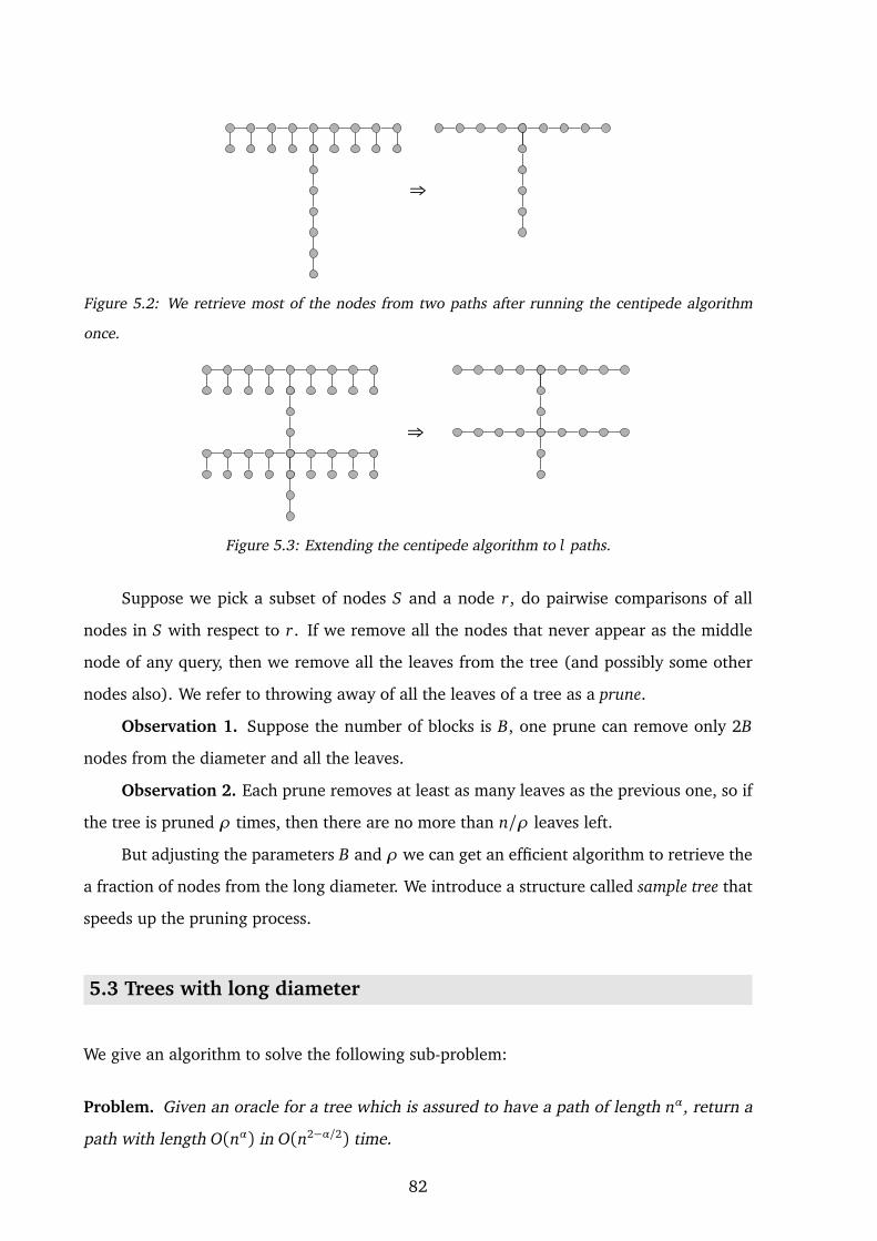
⇒
Figure 5.2: We retrieve most of the nodes from two paths after running the centipede algorithm
once.
⇒
Figure 5.3: Extending the centipede algorithm to l paths.
Suppose we pick a subset of nodes S and a node r, do pairwise comparisons of all
nodes in S with respect to r. If we remove all the nodes that never appear as the middle
node of any query, then we remove all the leaves from the tree (and possibly some other
nodes also). We refer to throwing away of all the leaves of a tree as a prune.
Observation 1. Suppose the number of blocks is B, one prune can remove only 2B
nodes from the diameter and all the leaves.
Observation 2. Each prune removes at least as many leaves as the previous one, so if
the tree is pruned ρ times, then there are no more than n/ρ leaves left.
But adjusting the parameters B and ρ we can get an efficient algorithm to retrieve the
a fraction of nodes from the long diameter. We introduce a structure called sample tree that
speeds up the pruning process.
5.3 Trees with long diameter
We give an algorithm to solve the following sub-problem:
Problem. Given an oracle for a tree which is assured to have a path of length nα, return a
path with length O(nα) in O(n2−α/2) time.
82

Input. The oracle for the tree T and the parameter α.
Apart from the input parameter α, the algorithm uses two internal parameters β and
ρ. We describe the algorithm assuming general terms and set their specific values later.
Definitions. The longest path in the tree T is called the necklace. A bead is a node on the
necklace. Given a set of nodes S from the tree T , a leaf in S is a node that does not appear
between any two nodes from S in T .
Intuition. The high-level idea is to collect a good fraction of beads. Imagine taking
the tree T and pruning it once. We lose all the leaves among which only two are beads.
If we continue to prune, the well spread out portions of the tree disappear at a rate much
faster than the beads. After sometime, the tree becomes so wilted that it is no more than a
collection of a few long paths. This makes it amenable to an exhaustive search for a long
path. The algorithm basically implements this idea.
Our algorithm runs in three-phases:
5.3.1 Phase I: Growing sample trees
Divide the nodes into blocks of size β each. So there are n/β blocks each containing a
sample of β nodes from the tree T . To avoid notational clutter, we omit the floors and
ceilings throughout the chapter. So n/β is really dn/βe.
Description of the sample tree
Let T1 denote the sample tree built using β nodes of the first sample as follows:
1. An arbitrary node is designated as the root r.
2. Let x and y be two nodes from the sample. Node x has node y as its parent if y is
the last node from the sample that appears before x on the path from r to x in T .
Note that every node has a unique parent, so T1 is in fact a tree (Fig. 5.4).
83

cd
e
f
g
h
ijk
l
m
r
r
l
m
j
k
ig
h
f
d
c e
T T1
Figure 5.4: T is the original tree and T1 is the sample tree.
Learning the sample tree
We can learn T1 from the oracle for T by using the naive quadratic algorithm that learns
each edge in O(n) time. We build a sample tree for each block this way.
Running Time.. Building one sample tree takes O(β2) time. So building n/β sample trees
takes O(nβ) time. We denote this time as tsample.
5.3.2 Phase II: Pruning
We prune each sample tree ρ times. Doing this ensures that many leaves are lost but not
many beads.
Key #1. Each sample tree contains at most two strands of the necklace.
Lemma 5.3.4. All the beads in the sample tree appear in at most two root-to-leaf paths.
Proof: Let node t be the junction at which the path
from the root meets the necklace. Let b1 b2 b3 . . . bm be
the beads in the sample that are to the right side of t.
Due to the way we have constructed the sample tree ev-
ery bi must have bi−1 as its parent (for i > 1). This
means all the bis appear on some root-to-leaf path con-
secutively. Similar argument holds for beads on the left
side of t.
t b1 b2 b3 bm
r
Lemma 5.3.5. At most 2nρ/β beads are lost after ρ prunes.
Proof: One prune can remove only two beads from a sample tree (Fig. 5.5). So at most
2n/β beads are lost from the all sample trees in one prune.
84

r
r
TiT
Figure 5.5: All the beads appear in at most two paths in the sample tree.
Lemma 5.3.6. The total number of leaves in all the sample trees is no more than n/ρ after
ρ prunes.
Proof: Let li denote the number of leaves in the sample tree Ti after ρ prunes. The number
of leaves in the sample tree cannot increase after a prune. Hence, each prune must have
removed at least li leaves. Since there were only β nodes in the sample tree liρ ¶ β . This
holds for all n/β samples trees, so (l1+ l2+ · · ·+ ln/β) ρ ¶ β × n/β
Running Time. Since the trees are already built, pruning is easy. Pruning ρ times is the
same as doing this: For each node x , if the most distant leaf in the subtree rooted at x is
less than ρ nodes away then remove x . Finding these distances takes linear time in the size
of the tree by dynamic programming. So overall pruning time is β × n/β = O(n). Since
this takes less time than building the sample trees, we ignore this time.
5.3.3 Phase III: Retrieving the Necklace
We will find the longest path in the subgraph induced by all the remaining nodes in the
pruned sample trees.
Key #2. Pruning the sample trees has a similar effect of pruning the actual tree. Consider
the tree T ′ induced by all the remaining nodes in the sample trees. Let l denote the number
of leaves in this tree.
Lemma 5.3.7. l ¶ 2n/ρ.
Proof: A node w in the pruned sample tree that appears between the root r and a leaf v
must appear on the path from r to v in T ′. Hence node w cannot be a leaf in T ′. So every
85

leaf in T ′ must either be a leaf or the root of some sample tree. A sample tree has only one
root, so there cannot be more roots than the leaves in a sample tree. So each sample tree
Ti can add at most 2li leaves to T ′. From Lemma 5.3.6 we have l ¶ 2n/ρ.
Claim 5.3.8. The longest path in a tree with n nodes and l leaves can be found in O(nl log n)
time using the oracle.
Proof: Note that we can learn the structure of a tree that has l leaves in O(nl log n) time.
One we learn the tree we find the longest path in it.
Running Time.. Since l ¶ 2n/ρ we can find the longest path in O(n2/ρ) time (ignoring
the log n factor). We denote this time as tsearch.
5.3.4 Tuning the parameters
Three parameters are under our control: one external parameter α and two internal pa-
rameters used by the algorithm: β and ρ. We will first set the internal parameters for a
given value of α.
Setting ρ: How long to prune?
We prune just enough number of times to retain half of the beads. Each prune discards at
most 2n/β beads (Lemma 5.3.5). How many times can we afford to prune so that at least
half of the beads remain?
ρ×2n
β
nα
2
ρ =βnα−1
4(5.1)
Setting β: What should be the sample size?
The parameter β controls the running time of the algorithm. There is a trade-off between
the running time of building the sample trees and exhaustive search. For example, if β is
a constant, then building the sample trees takes O(n) time but we can afford to prune only
constant number of times. This makes searching run in O(n2) time. On the other extreme,
if we set β to n then building the sample trees itself takes O(n2) time.
86

The running time of the algorithm is max(tsample, tsearch). We get the optimal running
time by choosing β such that tsample ≈ tsearch.
tsample = nβ
tsearch = n2/ρ Ignoring the constants
nβ = n2/ρ
β = 4n/βnα−1 From Eq. 5.1
β2 = 4n2−α
β = 2n1−α/2
Setting β = n1−α/2 gives the optimal running time of O(n2−α/2).
5.3.5 Finding the splitter
Let D be the diameter of the tree T . The above algorithm runs in O(n2−α/2) time and returns
a path of length at least D/2 if D is greater than nα. Note that the running time depends
only on the input parameter α and not on the true diameter of the tree. If we overestimate
α, then we get a shorter path in the same time. Hence, we can use this algorithm as a
probe to see if the tree has a long diameter. We call the median edge of a long path as a
splitter. For α = 0.8, the algorithm will return a splitter in O(n1.6) time if the diameter of
the tree is greater than 2n0.8. Combining this fact with the short-diameter algorithm gives
a sub-quadratic bound.
5.4 A Sub-Quadratic Algorithm
Run the long-diameter algorithm with α = 0.8. If it does not return a splitter, the diameter
of the tree must be less than 2n0.8. Learn the tree using the short-diameter algorithm. This
takes O(n1.8 log n) time. If we do get a splitter, divide and recurse on the subtrees. So for
any tree with n nodes we either get a splitter in O(n1.6) time or learn the tree in O(n1.8 log n)
time. The associated recurrence is given below:
87

T (n) =
O(n1.8 log n) if the diameter is less than 2n0.8
T (n− n0.8) + T (n0.8) + n1.6 otherwise
The solution to T (n) implies that a constant-degree tree can be learnt in O(n1.8 log n)
time.
5.5 Discussion
In this chapter, we have shown the process of applying WISE methodology to tree learning
problem. The key idea was to restrict the input instances to extremal trees. In all the
chapters, we have seen the role of extremality in graphs. But the principle has broader
applicability. In the next chapter, we show how it could be useful in the context of linear
programming.
88

Chapter 6
Extremality in Linear Programming
In the previous chapters, we saw how extremal graphs play a role in obtaining insight about
a problem. Here, we show how extreme points of a linear program play a similar role in
linear programming. Unfortunately, the application does not fit into the WISE methodology,
but uses only the extremality principle.
6.1 Motivation
Linear programming is an important topic in combinatorial optimization. There are several
good books on this topic that are aimed at senior undergraduate students. The current
texts on linear programming focus on computational aspects that need knowledge of linear
algebra as a prerequisite. It is well known that linear programming can also be used as
an analytical tool. For example, in theoretical computer science, duality is often used to
analyze approximation algorithms. Our plan is to introduce LPs by using the weaker form
of duality to solve Math-Olympiad problems. This style of introduction does not need linear
algebra as a prerequisite. Although our primary motive is exposition, all the proofs that are
presented are new.
Linear programming is a potential topic to highlight the usefulness of extremality. A
linear program (LP) defines a polytope in IRn. The ‘corners’ or the ‘tips’ of the polytope are
called extreme points. For example, if the polytope is a cube in IR3, then there are eight
extreme points. Just as extremal graphs have simple structures, the extreme points of LPs
also tend to have simple structures–this is what makes LPs effective as an analytical tool.
89
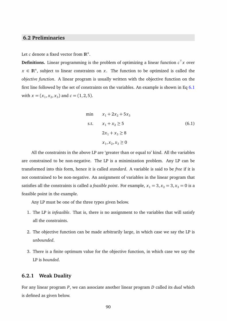
6.2 Preliminaries
Let c denote a fixed vector from IRn.
Definitions. Linear programming is the problem of optimizing a linear function c>x over
x ∈ IRn, subject to linear constraints on x . The function to be optimized is called the
objective function. A linear program is usually written with the objective function on the
first line followed by the set of constraints on the variables. An example is shown in Eq 6.1
with x = (x1, x2, x3) and c = (1,2, 5).
min x1+ 2x2+ 5x3
s.t. x1+ x2 ≥ 5 (6.1)
2x1+ x3 ≥ 8
x1, x2, x3 ≥ 0
All the constraints in the above LP are ‘greater than or equal to’ kind. All the variables
are constrained to be non-negative. The LP is a minimization problem. Any LP can be
transformed into this form, hence it is called standard. A variable is said to be free if it is
not constrained to be non-negative. An assignment of variables in the linear program that
satisfies all the constraints is called a feasible point. For example, x1 = 3, x2 = 3, x3 = 0 is a
feasible point in the example.
Any LP must be one of the three types given below.
1. The LP is infeasible. That is, there is no assignment to the variables that will satisfy
all the constraints.
2. The objective function can be made arbitrarily large, in which case we say the LP is
unbounded.
3. There is a finite optimum value for the objective function, in which case we say the
LP is bounded.
6.2.1 Weak Duality
For any linear program P, we can associate another linear program D called its dual which
is defined as given below.
90

Suppose P is written in the standard form:
minn∑
j=1
c j x j
s.t.n∑
j=1
ai j x j ≥ bi i ∈ 1, . . . , m (6.2)
x j ≥ 0 j ∈ 1, . . . , n
The following linear program is its dual:
maxm∑
j=1
b j y j
s.t.n∑
i=1
ai j yi ≥ c j j ∈ 1, . . . , n (6.3)
yi ≥ 0 j ∈ 1, . . . , m
We call the original LP P as the primal.
The weak duality theorem is the following:
Theorem 6.2.1. If x ′ and y ′ are feasible solutions for the primal and the dual respectively,
thenn∑
j=1
c j x′j ≥
m∑
j=1
bi y′j
The proof of weak-duality and the procedure to find the dual of any LP can be found
in the lecture notes by Michel Goemans [15] or any standard book on combinatorial op-
timization. What is important to us is the consequence of weak-duality. Apart from weak
duality, we use two corollaries that follow from weak-duality:
1. If the dual is unbounded, then the primal is infeasible.
2. If the dual is bounded, then the primal is feasible.
All the problems we consider involve finding a feasible point in the dual to prove
bounds or feasibility of the primal. We call this feasible point in the dual as a certificate.
Remark. The main reason why LP works as an analytical tool is because the certificates
have simple structures. Most often the certificate is an extremal point in the dual polytope.
91

6.2 LP-Method
For all the problems, we follow the three steps given below.
1. Formulate the given problem as an LP.
2. Take the dual.
3. Find a feasible point (certificate) in the dual. Invoke the weak-duality theorem.
The first two steps are trivial for all the problems. The last step is made easier by a
few tips which we describe below.
6.2.2 Tips
Tip 1: Scaling A constraint a>x ≤ b is said to be homogeneous if b is zero. If an inequality
is homogeneous, any feasible vector x multiplied by a positive number remains feasi-
ble. Scaling trick is useful in dealing with strict inequalities. A constraint (say) x > 0
can be written as x ≥ 1 sometimes.
Tip 2: Tightening When searching for a feasible point, it helps to make a group of inequal-
ities tight.
Tip 3: Zeroing Try setting all or some of the variables to zero or the same constant. This is
usually helpful if there are many variables, but only a few constraints (‘fat matrices’).
6.3 Problems
We illustrate the use of LPs to solve some Math Olympiad problems. In all cases, the solution
involves finding an extreme point of the dual and invoking the weak-duality theorem.
1 Baltic Olympiad 2006. For a sequence a1, a2, a3, . . . of real numbers it is known that
an = an−1 + an+2 for n = 2, 3,4, . . .. What is the largest number of its consecutive elements
that can all be positive?
Sol. We will show that the largest consecutive positive elements is 5. Without loss of
generality, we may assume that the largest such sequence begins with a1.
Upper bound. We first show that the length is less than six. The primal and corre-
sponding dual is given below.
92

min 0
s.t. a2− a1−a4 =0
a3− a2−a5 =0 (6.4)
a4− a3−a6 =0
ai ≥1 i ∈ [6]
max∑
βi
s.t. β1−α1 ≤0
β2+α1−α2 ≤0
β3+α2−α3 ≤0 (6.5)
β4+α3−α1 ≤0
β5−α2 ≤0
β6−α3 ≤0
Certificate. Set β2,β3,β4 to zero. The rest of the variables can be set to any positive
constant. This makes the dual unbounded which implies that the primal is infeasible.
Lower bound. To prove that a consecutive sequence of length five is possible, we
need to show that the following dual is feasible and bounded. Verify that the LP has only
all-zeros as the solution, hence the primal must be feasible when restricted to five numbers.
max5∑
i=1
βi
s.t. β1+α1 ≤0
β2+α1−α2 ≤0
β3+α2 ≤0 (6.6)
β4−α1 ≤0
β5−α2 ≤0
2 Folklore. Suppose bi ≥ 0 prove that :
a1+ · · ·+ an
b1+ · · ·+ bn≥
nmini=1
ai
bi(6.7)
93

Sol. Let us define f (x) as follows:
f (x) =a1 x1+ · · ·+ an xn
b1 x1+ · · ·+ bn xn
We will show that the RHS of (6.7) is the minimum value that f (x) attains in the
positive orthant. This proves the inequality since f (1) is equal to the LHS of (6.7). So we
have the following optimization problem:
mina1 x1+ · · ·+ an xn
b1 x1+ · · ·+ bn xns.t x i ≥ 0
By scaling trick, we may assume that the denominator takes the value 1 when f (x)
attains the minimum. This is always possible since bis are non-negative. Hence, we can
write the optimization problem as an LP:
minn∑
i=1
ai x i s.t.n∑
i=1
bi x i = 1 x i ≥ 0
The dual is:
max α s.t. biα≤ ai i ∈ [n]
Certificate. Setting α=min ai/bi, gives a feasible point.
Hence the value of the primal is bounded by min ai/bi.
3 IMO 1965. Consider the system of equations with unknowns x1, x2, x3.
a11 x1+ a12 x2+ a13 x3 = 0
a21 x1+ a22 x2+ a23 x3 = 0
a31 x1+ a32 x2+ a33 x3 = 0
The coefficients ai j of the following equations satisfy the following conditions.
1. Coefficients a11, a22, a33 are positive numbers.
2. The remaining coefficients are negative.
94

3. The sum of the coefficients in each equation is positive.
Prove that the only solution is x1 = x2 = x3 = 0.
Sol. Conditions (2) and (3) imply the first, so we can drop the first condition. We treat the
coefficients ai js as variables of the LP and x is as the coefficients. We scaling to deal with
positivity and negativity constraints.
min: 0 s.t
a11 x1+ a12 x2+ a13 x3 = 0 α1
a21 x1+ a22 x2+ a23 x3 = 0 α2
a31 x1+ a32 x2+ a33 x3 = 0 α3
−ai j ≥ 1 ∀i, j s.t i 6= j βi j
a11+ a12+ a13 ≥ 1 δ1
a21+ a22+ a23 ≥ 1 δ2
a31+ a32+ a33 ≥ 1 δ3
free variables: ai j ∀i, j s.t i 6= j
The dual (D) is as follows:
max δ1+δ2+δ3+∑
i 6= j βi j s.t (6.8)
x1α1+δ1 ≤ 0 a11
x2α2+δ2 ≤ 0 a22
x3α3+δ3 ≤ 0 a33
95

x2α1− β12+δ1 = 0 a12
x3α1− β13+δ1 = 0 a13
x1α2− β21+δ2 = 0 a21
x3α2− β23+δ2 = 0 a23
x1α3− β31+δ3 = 0 a31
x2α3− β32+δ3 = 0 a32
free variables: αis
We show that the dual 6.8 is unbounded if any of the x is is strictly positive. Since
the constraints are homogeneous, any scalar multiple of the feasible point is also feasible.
Hence, it is enough to show that there exists a feasible point with positive objective value.
We set the first group of constraints to equality (Tip 6.2.2).
δ1 =−x1α1
δ2 =−x2α2
δ3 =−x3α3
The second set of constraints now becomes:
β12 = α1(x2− x1)
β13 = α1(x3− x1)
β21 = α2(x1− x2)
β23 = α2(x3− x2)
β31 = α3(x1− x3)
β32 = α3(x2− x3)
96

Certificate. Suppose all the x is are not zero. Let x j have the largest positive value. We set
α j = −1 and all other αs to zero. This ensures that all the δs are non-negative. We need
to show that βs are also non-negative. Observe that x i − x j is non-positive for all values of
i since x j is chosen to be the largest positive number, hence all the βs are zero except the
ones that have α js on the right hand side of the equation.
4 IMO 1977. At a stockholders’ meeting, the board presents the month-by-month profits
(or losses) since the last meeting. “Note,” says the CEO, “that we made a profit over every
consecutive eight-month period.” “Maybe so,” a shareholder complains, “but I also see we
lost money over every consecutive five-month period!” What is the maximum number of
months that could have passed since the last meeting? The description of the problem is
taken from Peter Winkler’s book ‘Mathematical Puzzles’.
Sol. What we want is a sequence of numbers such that the sum of every eight consecutive
numbers is positive but sum of every five consecutive numbers is negative. We show that
the maximum length of such a sequence is 11.
First, we prove the upper bound by showing that a sequence of length 12 is not possi-
ble. Using the scaling tip, we can write the constraints as follows:
(Primal)
x1+ x2+ · · · + x7 + x8 ≥ 1 α1
x2+ x3+ · · · + x8 + x9 ≥ 1 α2
x3+ x4+ · · · + x9 + x10 ≥ 1 α3 (6.9)
x4+ x5+ · · · + x10+ x11 ≥ 1 α4
x5+ x6+ · · · + x11+ x12 ≥ 1 α5
97

x1+ x2+ x3+ x4+ x5 ≤−1 β1
x2+ x3+ x4+ x5+ x6 ≤−1 β2
x3+ x4+ x5+ x6+ x7 ≤−1 β3 (6.10)
x4+ x5+ x6+ x7+ x8 ≤−1 β4
x5+ x6+ x7+ x8+ x9 ≤−1 β5
x6+ x7+ x8+ x9+ x10 ≤−1 β6
x7+ x8+ x9+ x10+ x11 ≤−1 β7
x8+ x9+ x10+ x11+ x12 ≤−1 β8
All the variables in the primal are free. The dual is as follows:
max5∑
i=1
αi +8∑
j=1
β j
s. t.k∑
p=1
αp −k∑
q=1
βq = 0 k ∈ 1, . . . , 5
5∑
p=1
αp −k∑
q=k−4
βq = 0 k ∈ 6,7, 8
5∑
p=k−7
αp −8∑
q=k−4
βq = 0 k ∈ 9, . . . , 12
(6.11)
Certificate. We will show that the dual is unbounded. Since the constraints are
homogeneous it is enough to show that there exists a feasible point with positive objective
value. Notice that in all the constraints the number of αs is equal to the number of βs. This
means that the we can set all the variables to 1 and satisfy the constraints. This shows that
the primal is infeasible. Hence, there is no profit sequence of length 12. We will prove that
there exists a profit sequence of length 11. The primal in this case will remain the same
except that we drop the last constraint in Eq. 6.9 and 6.10. The corresponding dual is given
98

below. The constraints are shown after some simplification.
max5∑
i=1
αi +8∑
j=1
β j
s. t. α1 = β1 x1
α2 = β2 x2
α3 = β3 x3
α4 = β4 x4
β5 = 0 x5
α1 = β5 x6
α2 = β6 x7
α3 = β7 x8
α4 = β5 x9
α4 = β6 x10
α4 = β7 x11
(6.12)
Certificate. The constraint β5 = 0 forces all the variables to be zero. Hence, all-zeroes is
the only feasible solution to the dual. Since the dual is feasible and bounded the primal
must be feasible which implies that there exists a profit sequence of length 11.
5 Engel Chap. 9 [8]. Let a1, . . . , an be a sequence of real numbers such that a0 = an = 0
and ak−1− 2ak + ak+1 ≥ 0 for k = 1,2, 3, . . . , n− 1. Prove that ak ≤ 0.
Sol. We need to bound the maximum value of ak under the given constraints. Let us
associate dual variables α0 and αn with equality constraints and βi with the ith inequality.
The dual is as follows:
99

min 0
s.t. β1−α0 = 0
− 2β1+ β2 = 0
β1− 2β2+ β3 = 0
β2− 2β3+ β4 = 0
...
βk−1− 2βk + βk+1 = −1
...
βn−2− 2βn−1 = 0
αn− βn−1 = 0
free variables: α0 and αn
Since the objective is zero, we have to show that the equations are feasible. The basic
idea is to make use of the following observation: if βis are in an arithmetic progression all
but one of the equations are satisfied. We show that combining two A.P.s suffices to fix the
problem.
Lemma 6.3.1. There exists two positive values p and q such that setting βi = ip for (1 ≤
i ≤ k) and βn− j = jq for (1≤ j ≤ n− k) satisfies all the equations.
Proof: Observe that βk is both kp and and (n− k)q, so we need:
kp = (n− k)q
For any values of p and q, all the equations in the dual, except possibly the one correspond-
ing to ak, are satisfied. That equation will also be satisfied if:
(k− 1)p− 2kp+ (n− k− 1)q =−1
Since kp = (n − k)q, both p and q must have the same sign. Adding the previous two
equations gives p+q = 1, so p and q must be positive. Hence, we can find their values and
substitute to get the values of βs.
100
6 Matematikai Lapok, Budapest. Show that if 2n+ 1 real numbers have the property
that the sum of any n is less than the sum of the remaining n+ 1, then all these numbers
are positive. Titu Andreescu’s book ‘Mathematical Olympiad Challenges’.
Sol. We first solve the problem for the case when n = 3. This gives an idea to solve the
general case. Without loss of generality, assume that x1 is the minimum element of the
sequence. We need to show that x1 is positive. Using the scaling trick, we can write the
constraints as follows:
min x1
s.t. + x1+ x2−x3 ≥1
+ x2− x2+x3 ≥1
− x3+ x2+x3 ≥1
The dual is as follows:
min α1+α2+α3
s.t. +α1+α2− α3 =1
+α2−α2+ α3 =0
−α3+α2+ α3 =0
What is a feasible solution to the dual? Observe that setting α1 = 1/2, α2 = 1/2 and
α3 = 0 satisfies the constraints. Since the objective value is now positive, we have proved
the statement for n = 3. The special case gives a way to solve the general case which is
captured by the following lemma.
Lemma 6.3.2. There is always a dual solution in which two variables are set to 1/2 and
the rest of them to zero.
Proof: Let S =
x2, . . . , x2n
. Let A and B = S \ A be any two subsets with |A| = |B| = n.
Let variables αi and α j correspond to primal constraints x1+A− B ≥ 1 and x1+ B−A≥ 1,
respectively. We set αi and α j to 1/2. We use this as a certificate.
Remark. The dual gives an insight to solve the problem combinatorially. The two con-
straints mentioned in the proof are sufficient to show that x1 ≥ 1.
7 IMO 2007. Real numbers a1, . . . , an are given. For each i, (1≤ i ≤ n), define
101

di =maxa j | 1≤ j ≤ i −mina j | i ≤ j ≤ n
and let d =maxdi|1≤ i ≤ n.
Prove that for any real numbers x1 ≤ x2 ≤ · · · ≤ xn the following relation holds:
max|x i − ai| | 1≤ i ≤ n ≥d
2. (6.13)
Sol. The problem can be formulated as an LP:
min t
s.t. t ≥+ x i − ai i ∈ [n] αi
t ≥− x i + ai i ∈ [n] βi (6.14)
x i+1≥x i i ∈ [n− 1] γi
All the variables are free. We need to show that the value of the above LP is at least
d/2. The dual is the following:
maxn∑
i=1
ai(βi −αi)
s.t.n∑
i=1
(αi + βi) =1
β1−α1− γ1 =0
βi −αi − γi + γi−1=0 2≤ i ≤ n− 1
βn−αn− γn−1 =0
Let p and q, be the indices for which ap−aq is maximum. This quantity is equal to d if
p < q. We need to prove that the dual has a feasible solution whose value is d/2. This can
be done by setting βp = 1/2 and αq = 1/2 and the rest of αs and βs to zero. Now we need
to show that there exists a feasible solution within this assignment. The values of γs are
determined by the values of αs and βs. Variables γps through γq−1 are set to 1/2, while the
rest of them are zero. Since all the variables are non-negative and the value of the objective
is d/2, we have proved the relation given in (6.13).
102

8 IMO 1979. Determine all real numbers a for which there exists positive reals x1, . . . , x5
which satisfy the relations
5∑
k=1
kxk = a5∑
k=1
k3 xk = a25∑
k=1
k5 xk = a3
Sol. Since we only need to check the feasibility of the equations, the dual can either be
considered as a minimization or maximization problem. Here is one possible dual:
max αa3+ βa2+ γa
s.t. i5α+ i3β + iγ≤0 i ∈ [5]
Lemma 6.3.3. If a = k2 for some k ∈ [5]∪ 0, then the dual is feasible and bounded. For
any other value, the dual is unbounded.
Proof: Case 1: Suppose a is negative. The dual is unbounded. We set α = β = 0 and
γ=−∞.
Case 2: Suppose a = k2 for some k ∈ [5]. The objective is same as the L.H.S of one
of the constraints. Since each constraint is at most zero, the objective is upper bounded by
zero. Setting the dual variables to zero would give a feasible point.
Case 3: Suppose a is positive but is not equal to k2 for any k ∈ [5]. Since the inequalities
are homogeneous it is enough show that there exists a feasible point with positive objective
value. We will prove that there exists a feasible point with positive objective value in which
γ=−1. We rewrite the LP as follows:
max αa2+ βa− 1
s.t. i4α+ i2β − 1≤ 0 i ∈ [5]
Suppose k2 < a < (k+ 1)2 for some k ∈ [4]. We set the constraints corresponding to
i = k and i = k+1 to equalities. We prove that doing so satisfies all the other constraints and
also makes the objective positive. Let α′ and β ′ be the values that α and β take respectively,
when we solve these two equations. Consider the quadratic p(x) = α′x2 + β ′x − 1 = 0
(Fig. 6.1). Note that p(k2) = 0 and p((k + 1)2) = 0 and p(a) > 0. p(a) has the form of
103

12 a 22
x
y
Figure 6.1: If a is in between two roots, then the objective is positive and the constraints are
negative.
objective function, so the objective is positive. The quadratic has negative values for all x
lesser than k2 or greater than (k+ 1)2, hence the other constraints are also satisfied.
9 Folklore. Prove that a 10x10 board cannot be tiled using 4x1 tiles.
Sol. Assume that the bottom-left corner denotes the cell (1, 1). Let hi, j denote the horizontal
tile that covers the cell (i, j) and three cells to its right. Similarly let vi, j denote the vertical
tile that covers the cell (i, j) and three cells above it. Let T be the set of all possible tiles,
that is, T =¦
h1,1, . . . , h7,10
©
∪¦
v1,1, . . . , v10,7
©
.
We formulate the problem as follows: What is maximum number of non-overlapping
tiles we can place? If a tiling exists then the answer must be 25. We show that it not
possible to place more than 24 non-overlapping tiles.
LP-formulation. We want to pick the maximum number of tiles subject to the constraint
that no two tiles overlap. We ensure this by saying that among all the tiles that cover a
cell c, at most one should be picked. The corresponding linear program is given below. C
denotes the set of all cells and Tc denotes the tiles in T that cover the cell c.
max:∑
t∈T
t
∑
t∈Tc
t ≤ 1 ∀c ∈ C
The dual will have one variable for each cell. Let C ′ denote the set of dual variables.
Let C ′t ⊂ C ′ denote the dual variables that correspond to the cells covered by the tile t. The
dual is given below.
104

Figure 6.2: The dual variables corresponding to shaded cells are set to 1 and the rest to 0. This
assignment gives a feasible solution with objective value 24.
.
min:∑
c∈C ′c
∑
c∈C ′t
c ≥ 1 ∀t ∈ T
Certificate. There is a feasible solution to the dual with objective value 24. We set all the
dual variables corresponding to the shaded cells in Fig. 6.2 to 1 and the rest to zero. Since
there are 24 shaded cells, the objective has value 24. To check for feasibility notice that
every possible tile contains exactly one shaded cell, so all the dual constraints are satisfied
with equality.
Remark. We can give a direct counting proof using the certificate. Suppose, for contradic-
tion’s sake, there was a tiling of the board. Then each tile would be placed on exactly one
shaded cell (Fig. 6.2). This impossible since there are only 24 shaded cells. The problem
appears in a nice survey paper on tilings by Ardila and Stanley [1]. The combinatorial proof
given in their paper is different from ours.
6.4 Discussion
Most textbooks and lectures use examples like matching, shortest path and network flow as
introductory examples for duality. These examples rely on linear algebra in some way. We
have given simpler illustrative examples for weak-duality. In all the problems we discussed,
the key to the solution was finding a certificate with a simple structure. This is also one of
the keys to solve a few research problems. Popular examples can be found in [33].
105

106

Chapter 7
Conclusion
All mathematicians are familiar with the concept of an open research problem.
I propose the less familiar concept of an open exposition problem. Solving an
open exposition problem means explaining a mathematical subject in a way that
renders it totally perspicuous. Every step should be motivated and clear; ideally,
students should feel that they could have arrived at the results themselves.
-Timothy Chow [5]
7.1 Direct proofs vs WISE
We have seen that in all three applications the use of WISE methodology is invisible in
the final solutions. For example, the anchor method can be described solely in terms of
extremal discrepancy graphs. We can describe query lower bounding technique solely in
terms of extremal critical graphs. It is a convention in textbooks to describe solutions in a
way that makes them easy to verify. We feel that from an educational point of view this
does not do justice to the craft of designing algorithms. Hence, we have chosen a style of
exposition that makes the source of ideas transparent to the student.
There are many problems in computer science with short clever results but for which
no exposition exists that describe their route to discovery. It would be interesting to give
such an account for such problems using the WISE methodology. A few possible candidate
problems are listed below:
• Linear-time median finding algorithm.
• Katona’s proof of Erdos-Ko-Rado theorem.
107

Problem Solution
WISE
Figure 7.1: Direct proofs are simpler to explain but deriving via WISE, though long-winded, makes
the process of discovery transparent.
• Karger’s randomized min-cut algorithm.
• Schoning’s algorithm for 3SAT.
• Perceptron algorithm for finding a separating plane.
7.2 Problems related to teachability of WISE
Among the steps discussed in WISE, we believe the following two are critical:
1. Formulating a set of weak candidate problems There are hardly any questions in text-
books whose objective is to come up with a list of weaker problems for a given prob-
lem. Most instructors also assume that this step will be implicitly done as part of
solving a problem.
2. Coming up with multiple proofs In some instances, we may have to come up with
multiple proofs for the weak problem before finding the proof that generalizes. This
is also a skill that is not given due importance in the textbooks.
108

References
[1] Federico Ardila and Richard P Stanley. Tilings. The Mathematical Intelligencer,
32(4):32–43, 2010. 105
[2] Sanjeev Arora and Boaz Barak. Computational complexity: a modern approach. Cam-
bridge University Press, 2009. 59, 69, 70, 72
[3] Michael Ben Or. Lower bounds for algebraic computation trees. In Proceedings of the
fifteenth annual ACM Symposium on Theory of Computing (STOC), pages 80–86. ACM,
1983. 57, 58
[4] S. K. Chang and A. Gill. Algorithmic solution of the change-making problem. J. ACM,
17:113–122, January 1970. 54
[5] T.Y. Chow. A beginner’s guide to forcing. Communicating Mathematics, Contemp.
Math, 479:25–40, 2009. 107
[6] T. H. Cormen, C. E. Leiserson, R. L. Rivest, and C. Stein. Introduction to Algorithms.
The MIT Press, 2nd edition, 2001. 2, 3, 23, 57, 58, 59
[7] Sanjoy Dasgupta, Christos H Papadimitriou, and Umesh Vazirani. Algorithms.
McGraw-Hill, Inc., 2006. 2
[8] Arthur Engel. Problem-solving strategies. Springer New York, 1998. 4, 99
[9] Jeff Erickson. http://web.engr.illinois.edu/~jeffe/teaching/algorithms/
notes/99-recurrences.pdf. Last Accessed Nov 10, 2014. 2
[10] Jeff Erickson. http://www.cs.uiuc.edu/~jeffe/teaching/algorithms/notes/
29-adversary.pdf. Last Accessed Jan 10, 2014. 59, 69
109

[11] Jeff Erickson et al. Lower bounds for linear satisfiability problems. Chicago Journal of
Theoretical Computer Science, 8:1999, 1999. 57, 59
[12] Anka Gajentaan and Mark H Overmars. On a class of o(n2) problems in computational
geometry. Computational geometry, 5(3):165–185, 1995. 59
[13] M. R. Garey and D. S. Johnson. Computers and Intractability: A Guide to NP-
Completeness. Freeman, San Francisco, CA, USA, 1979. 34
[14] D. Ginat. Gaining algorithmic insight through simplifying constraints. JCSE Online,
2002. 10
[15] Michel Goemans. http://math.mit.edu/~goemans/18433S13/polyhedral.pdf.
Last Accessed Aug 10, 2014. 91
[16] Teofilo Gonzalez and Sartaj Sahni. Open shop scheduling to minimize finish time. J.
ACM, 23:665–679, October 1976. 54
[17] Sudipto Guha and Samir Khuller. Approximation algorithms for connected dominat-
ing sets. Algorithmica, 20:374–387, 1996. 40
[18] M Jagadish and Sridhar Iyer. A method to prove query lower bounds. In Proceedings
of the 2014 conference on Innovation & technology in computer science education, pages
81–86. ACM, 2014. 112
[19] David S. Johnson. Approximation algorithms for combinatorial problems. In Pro-
ceedings of the fifth annual ACM Symposium on Theory of Computing, STOC ’73, pages
38–49, New York, NY, USA, 1973. ACM. 34
[20] Jeff Kahn, Michael Saks, and Dean Sturtevant. A topological approach to evasiveness.
Combinatorica, 4(4):297–306, 1984. 72
[21] Jon Kleinberg and Éva Tardos. Algorithm Design. Addison Wesley, second edition,
2006. 2, 3, 17, 25, 57
[22] FK Lester and PE Kehle. From problem solving to modeling: The evolution of thinking
about research on complex mathematical activity. Beyond constructivism: Models and
modeling perspectives on mathematics problem solving, learning, and teaching, pages
501–517, 2003. 1
110

[23] Jagadish M. An approximation algorithm for the cutting-sticks problem. Information
Processing Letters, 115(2):170–174, 2015. 112
[24] Jagadish M. and Sridhar Iyer. A method to construct counterexamples for greedy
algorithms. In Proceedings of the 2012 Conference on Innovation and Technology in
Computer Science Education, pages 238–243, 2012. 23, 112
[25] Jagadish M. and Sridhar Iyer. Problem-solving using the extremality principle. In
Proceedings of the 2014 Conference on Innovation and Technology in Computer Science
Education, pages 87–92, New York, NY, USA, 2014. ACM. 112
[26] Jagadish M. and Anindya Sen. Learning a bounded degree tree using separator
queries. In Algorithmic Learning Theory, 2013. 73, 112
[27] G. Polya. How to Solve It - a New Aspect of Mathematical Method. Princeton University
Press, Princeton, 2 edition, 1957. 2, 4, 10
[28] Shuichi Sakai, Mitsunori Togasaki, and Koichi Yamazaki. A note on greedy algorithms
for the maximum weighted independent set problem. Discrete Appl. Math., 126:313–
322, March 2003. 25
[29] Sally A. Goldman and Kenneth J. Goldman. Adversary Lower Bound Technique. http:
//goldman.cse.wustl.edu/crc2007/handouts/adv-lb.pdf. Last Accessed Jan 10,
2014. 59, 69
[30] Alan H Schoenfeld. Teaching problem-solving skills. American Mathematical Monthly,
pages 794–805, 1980. 1, 2
[31] Alan H Schoenfeld. Mathematical problem solving. ERIC, 1985. 1
[32] Bharath. Sriraman and Lyn D English. Theories of mathematics education: seeking new
frontiers. Springer, 2010. 1, 2
[33] Vijay V Vazirani. Approximation algorithms. springer, 2001. 105
[34] Douglas B. West. Introduction to Graph Theory. Prentice Hall, 2 edition, September
2000. 34, 57
[35] Peter Winker. Mathematical puzzles: a connoisseur’s collection. CRC Press, 2003. 15
111

Thesis-Related Conference Publications
1. “A method to construct counterexamples for greedy algorithms” (with Prof. Sridhar
Iyer) published in ITiCSE 2012 [24].
2. “A method to prove query lower bounds” (with Prof. Sridhar Iyer) published in ITiCSE
2014 [18].
3. “Learning a bounded degree tree using separator queries” (with Anindya Sen) pub-
lished in Algorithmic Learning Theory (ALT) 2013 [26].
4. “Problem-solving using extremality principle” (with Prof. Sridhar Iyer) published in
ITiCSE 2014 [25].
Journal Publication
1. “An approximation algorithm for the cutting-sticks problem” in Information Processing
Letters. Vol.115(2), 2015. [23]. This paper is unrelated to the thesis.
112

Acknowledgments
I am grateful to my advisor, Prof. Sridhar Iyer, for being a great source of support and
insight. I thank him for giving me the freedom to work on problems of my choice and at my
own pace. His insistence on not losing the big picture is what finally helped me to shape
the thesis. Above all, I thank him for making the journey so enjoyable.
I thank Prof. Krithi Ramamritham for his encouragement during the initial days of my
PhD. His support helped me decide to work in the area of CS education. I thank Prof. Sun-
dar Vishwanathan for initiating me to research. Whatever I learnt under his guidance has
served me in good stead. Taking Prof. Sahana Murthy’s introductory course on research
methods and interacting with students of ET group helped me gain fluency in reading pa-
pers related to education.
I am thankful to Professors Milind Sohoni and Varsha Apte for being on my research
progress committee and for giving regular feedback. I am grateful to Prof. Madhavan
Mukund for a thorough review of the thesis.
I have learnt as much from my friends in the department as I have from teachers. I
believe that informal conversations have great value. At the very least, discussing a fun
topic over dinner can make mess food more palatable. In fact, one of the results in the
thesis grew out of such discussions with my friend Anindya. My stay at IIT was sweetened
due to many friends: Vishal, Jinesh, Soumitra, Prasad, Srinivas, Karthik, Abhisekh, Prateek,
Bharath, Vasudevan, Ashish, Suresh Kumar, Arjun, Renuka, Suresh S., Ayush, Ruta, Jugal,
Sandeep to name a few. I thank them all and others who I may have inadvertently forgotten.
Finally, I thank my family for their constant support and encouragement. I dedicate
this thesis to my parents.
Date: Jagadish M.


![Design Methodology , Problem Solving and Creative Thinking [Autosaved]](https://img.pdfslide.us/doc/110x75/55cf977c550346d03391de9f/design-methodology-problem-solving-and-creative-thinking-autosaved.jpg)


