School of Mathematics and Systems Engineering

Reports from MSI - Rapporter från MSI

A Probabilistic Part-of-Speech Taggerwith Suffix Probabilities

Johan Hall

April2003

MSI Report xxxxxVäxjö University ISSN xxxx-xxxxSE-351 95 VÄXJÖ ISRN VXU/MSI/DA/E/--xxxxx/--SE

A Probabilistic Part-of-Speech Tagger with Suffix

Probabilities

Johan HallMaster’s Thesis

April 2, 2003

Abstract

This master’s thesis deals with the problem of automatic part-of-speech tagging,where the main task is to assign the correct part-of-speech to each word in atext.A part-of-speech tagger is used in many language technology applications asa first step in a longer process such as grammar checking, machine translation,information extraction and information retrieval.

The part-of-speech tagger developed in this thesis is based on probabilitytheory. The two main probabilistic models used are the lexical model andthe contextual model. To estimate the probabilities the tagger uses supervisedmachine learning and trains the model using a collection of texts called corpus.

This thesis defines and empirically evaluates models based on suffix proba-bilities for dealing with the problem of unknown words part-of-speech tagger.Furthermore, it describes an efficient implementation of a part-of-speech taggerwith suffix probabilities, using a trie data structure. Around 95% accuracy rateis reported and the part-of-speech tagger tags about 70000 tokens in a second.

Contents

1 Introduction 2

2 Background 42.1 Part-of-Speech Tagging . . . . . . . . . . . . . . . . . . . . . . . 42.2 Probabilistic Part-of-Speech Tagging . . . . . . . . . . . . . . . . 62.3 Hidden Markov Models . . . . . . . . . . . . . . . . . . . . . . . 7

2.3.1 Lexical model . . . . . . . . . . . . . . . . . . . . . . . . . 72.3.2 Contextual model . . . . . . . . . . . . . . . . . . . . . . 8

2.4 Smoothing . . . . . . . . . . . . . . . . . . . . . . . . . . . . . . . 82.4.1 Additive Smoothing . . . . . . . . . . . . . . . . . . . . . 82.4.2 Linear Interpolation . . . . . . . . . . . . . . . . . . . . . 92.4.3 Choice of smoothing method . . . . . . . . . . . . . . . . 9

2.5 Viterbi . . . . . . . . . . . . . . . . . . . . . . . . . . . . . . . . . 9

3 Tagging models 113.1 Baseline model . . . . . . . . . . . . . . . . . . . . . . . . . . . . 113.2 Lexical models . . . . . . . . . . . . . . . . . . . . . . . . . . . . 133.3 Contextual models . . . . . . . . . . . . . . . . . . . . . . . . . . 16

4 Implementation 184.1 Preliminaries . . . . . . . . . . . . . . . . . . . . . . . . . . . . . 184.2 Lexical model . . . . . . . . . . . . . . . . . . . . . . . . . . . . . 204.3 Contextual model . . . . . . . . . . . . . . . . . . . . . . . . . . . 214.4 Segmentation and Viterbi . . . . . . . . . . . . . . . . . . . . . . 224.5 Tokenizer . . . . . . . . . . . . . . . . . . . . . . . . . . . . . . . 244.6 Tagset . . . . . . . . . . . . . . . . . . . . . . . . . . . . . . . . . 244.7 Options . . . . . . . . . . . . . . . . . . . . . . . . . . . . . . . . 24

5 Evaluation 265.1 Corpus data . . . . . . . . . . . . . . . . . . . . . . . . . . . . . . 265.2 Evaluation . . . . . . . . . . . . . . . . . . . . . . . . . . . . . . . 265.3 Results . . . . . . . . . . . . . . . . . . . . . . . . . . . . . . . . . 27

5.3.1 Lexical model . . . . . . . . . . . . . . . . . . . . . . . . . 275.3.2 Contextual model . . . . . . . . . . . . . . . . . . . . . . 295.3.3 Final test . . . . . . . . . . . . . . . . . . . . . . . . . . . 31

5.4 Discussion . . . . . . . . . . . . . . . . . . . . . . . . . . . . . . . 32

6 Conclusion 34

1

A The SUC small tagset 37

B The SUC large tagset 38

2

Chapter 1

Introduction

This master’s thesis deals with a common problem in the area of languagetechnology: How can we automatically assign parts-of-speech to words in atext? Examples of parts-of-speech are noun, adjective and verb. The resultof a part-of-speech tagging maybe in itself is not so interesting, but there aremany applications in language technology where this information is useful. Forexample, a grammar checking application maybe needs to know the part-of-speech of each word as a first step in the analysis process.

At first sight this problem may sound trivial, but it is actually very hard tosolve. In fact there is no known method that solves the problem with completeaccuracy and it may well be impossible to assign a part-of-speech to each word ina text correctly. There are studies which have tested two humans with linguistictraining on this task, and which have found that they disagree on 2 percent ofthe words [13]. It is therefore reasonable to restrict the problem a little. Howcan we automatically assign parts-of-speech to words in a text with the highestpossible accuracy rate?

In this thesis I define, implement and empirically evaluate a probabilisticsolution to the part-of-speech tagging problem for Swedish text. This means thatI need to define and implement probabilistic models to cope with the problem.A big help in this approach is to have access to tagged text, which means thatevery word and punctuation mark in the text has information about its part-of-speech, or lexical category. A large collection of such text is called corpusand I will use the Stockholm-Umea Corpus (SUC) of written Swedish in thiswork [6, 10]. I will in this report use the term tag which refers to a lexicalcategory or part-of-speech in the context of a particular corpus. The termtagset will also be used and refers to the set of all tags which the part-of-speechtagger can use to tag a text. There is no standard tagset for Swedish so I willuse the same tagsets that the Stockholm-Umea Corpus (SUC) uses.

The purpose of this master’s thesis is to develop part-of-speech tagger forSwedish which is both accurate and efficient. I will investigate if a probabilisticmodel with word suffixes in combination with well known models can be usedto achieve the complementary goals of accuracy and efficiency.

My primary goal is to define probabilistic models which result in a 95 percentaccuracy when tagging untagged text with the Stockholm-Umea Corpus. Thesemodels should be implemented in such a way that the tagger is able to tag 20000tokens per second on average.

3

Hopefully the tagger will be used in the future and this means that the taggermust be easy to change and extend. A secondary goal when implementing thetagger is to design and implement it in such a way that new modules can beinserted easily, such as a new tokenizer or the support of new corpus resources.It is also important that the tagger is easy to use.

The primary goals will be carefully evaluated in chapter 5. The secondarygoals will not be evaluated in the strict sense of doing user tests. How the sec-ondary goals are accomplished will be discussed in chapter 4. The implementedpart-of-speech tagger is called MALT tagger after the name of the group MALT(Models and Algorithms for Language Technology) at Vaxjo University workingwith language technology.

The thesis is organized as follows. Chapter 2 presents the background the-ory which explains the models and algorithms needed. Chapter 3 explains themodels used in the practical work of the thesis. Implementation of the part-of-speech tagger is presented in chapter 4. Empirical evaluation of the modelsexplained in chapter 3 is presented in chapter 5. Finally, chapter 6 is devotedto the main conclusions of the study.

4

Chapter 2

Background

2.1 Part-of-Speech Tagging

The task of assigning to every word in a text a part-of-speech like noun or verbis called part-of-speech tagging. Consider the following Swedish sentence:

Mot slutet av sommaren 1988 hade hon sina forsta egnalangritter genom smalandsskogarna.

The output of a part-of-speech tagger is a sequence of parts-of-speech attached toevery word and punctuation mark. In table 2.1, we can see that every token i.e.

Table 2.1: Example of tagged textWord Part-of-speech Morphosyntactic

propertiesMot PPslutet NN NEU SIN DEF NOMav PPsommaren NN UTR SIN DEF NOM1988 RG NOMhade VB PRT AKThon PN UTR SIN DEF SUBsina PS UTR/NEU PLU DEFforsta RO NOMegna JJ POS UTR/NEU PLU

IND/DEF NOMlangritter NN UTR PLU IND NOMgenom PPsmalandsskogarna NN UTR PLU DEF NOM. MAD

word or punctuation mark, has a tag attached to it, listed in the second columnof the table. Each tag refers to a part-of-speech and the tagset used here, aswell as the example sentence, is taken from the Stockholm-Umea Corpus [6, 10].A corpus is a collection of texts from different areas such as newspaper text

5

and scientific articles. A corpus in most cases contains extra information aboutevery word such as its part-of-speech and morphosyntactic properties. Often thetagset is extended to include also morphosyntactic properties such as numberand gender for nouns, which is what we find in the third column in Table 2.1.The full tagsets with and without morphosyntactic features are described inappendix A and B.

Part-of-speech tagging can be used in many applications as one step in alonger process, example in machine translation, information retrieval, informa-tion extraction and grammar checking. If we want to translate the Swedish wordklippa to English, the word can be translated as either cut or cliff in English. Ifwe know that the word klippa is a verb the translation is easier: cut. Informa-tion extraction applications are using patterns for extracting information fromtext and often make reference to parts-of-speech in templates [2].

Because a natural language like Swedish contains many ambiguous wordsregarding parts-of-speech, it is hard or impossible to construct a tagger thattags with an accuracy of 100 percent. Consider the following Swedish sentences:

Jag ska resa till Australien.Min resa till Australien var underbar.

The word resa has two possible parts-of-speech depending on context: noun orverb. In the first sentence the word is a verb and in the second sentence theword is a noun. Even if we list all words in a language with their possible parts-of-speech we still have the problem with ambiguous words. When we constructa part-of-speech tagger we must obtain information about the context and thendevelop a method of disambiguating these hard words.

A natural language has evolved as a means for humans to communicatewith each other and a language is usually open in the sense that it developsover time. A natural language is in constant evolution. Thus, in addition to thebasic ambiguity the following factors make part-of-speech tagging difficult:

• Unknown words: Over time we can not expect to have a complete listof every word in a natural language. New words become popular, otherwords will be forgotten and other words will get a new spelling. We mustfind a solution for handling unknown words.

• Indeterminacy : Since a natural language is an open and evolving system,there is sometimes disagreement about which tag is the correct one evenamong human experts.

• Noise: There are also errors in the data resources which help us buildlanguage technology applications.

There are parts-of-speech which usually only contain a small number of words,such as conjunctions and prepositions, and these parts-of-speech are known asclosed classes. It is not likely that new words will be added frequently to theclose classes. There are however closed classes which contain a large numberof words such as numerals. The opposite of closed classes are the open classescontaining parts-of-speech which usually have thousands of members and wherenew members are added continuously, such as nouns and verbs. The distinctionclosed and open classes is relevant when handling unknown words, since theseare more likely to belong to open classes [9].

6

There are several different approaches to solving the problem of part-of-speech tagging:

• Rule-based part-of-speech tagging : The first attempts to do part-of-speechtagging were based on a two step approach. In the first step every wordwas assigned a list of potential parts-of-speech from a dictionary. In thenext step the text was processed by a list of hand-written disambiguationrules. After applying every rule the list was reduced to only containingone part-of-speech for each word [9, 2].

• Probabilistic part-of-speech tagging : This approach uses probabilistic mod-els to determine the most probable part-of-speech sequence for a givenword sequence. The models usually incorporate probabilities of words inrelation to the parts-of-speech and of parts-of-speech in relation to otherparts-of-speech [9].

• Transformation-based part-of-speech tagging : Transformation-based, tag-ging often also called Brill tagging, combines the benefits of both rule-based and probabilistic parts-of-speech tagging. Usually the tagger firstassigns to every word the most likely part-of-speech. This approach willintroduce several errors. The next step is to correct as many errors aspossible by applying transformation rules that the tagger has learned [2].

2.2 Probabilistic Part-of-Speech Tagging

A popular solution is known as probabilistic part-of-speech tagging and uses aprobabilistic model during the tagging phase. The tagger tries to find the mostprobable part-of-speech sequence for a given word sequence. In most cases theprobabilistic model consists of a lexical and a contextual model. In the lexicalmodel, every word has a set of probable parts-of-speech. However, only usinga lexical model is not enough to tag with high accuracy. We also need a modelto capture the context of tags. In the contextual model, every part-of-speech isconditioned on its neighboring parts-of-speech.

We can use supervised machine learning to generate the lexical and thecontextual model. To do so we need manually annotated data. In other words,we need corpus where a part-of-speech is attached to every token. One way touse the corpus is to count every occurrence of a particular word tagged witha particular tag and use this frequency to compute probabilities for the lexicalmodel. By counting the occurrences of a particular in the context of othertags, we can compute corresponding frequencies for the contextual model. If notagged corpus is available from which we can obtain the probabilities needed, wecan use unsupervised learning. There is an algorithm called Baum-Welch thatis suitable when no tagged corpus is available [2]. Whether we use supervisedor unsupervised learning the corpus used to derive probabilities is referred to asthe training corpus.

Supervised learning in most cases is the best way to obtain the probabilitiesneeded. Merialdo [14] suggests that the optimal strategy to build the bestpossible model for tagging is the following:

• Use as much tagged text as possible.

7

• Compute the relative frequencies to obtain an initial model.

• Collect as much untagged text as possible.

• Use the Baum-Welch algorithm on the untagged text in several iterations.If the tagging quality degrades when using the new model with untaggedtext stop using it.

2.3 Hidden Markov Models

Markov models are state-space models that can be used to model a sequenceof random variables that are not necessarily independent. The most commonmodel used by probabilistic taggers is the n-class model which can be imple-mented as a hidden markov model (HMM) with states corresponding to sequenceof parts-of-speech and output symbols corresponding to tokens [14]. In a HMM,we do not know the state sequence that the model passes through, but onlythe output sequence which is a probabilistic function of it. In a part-of-speechtagger application we define the problem more formally as follows. For a givenstring of words w1, ..., wk, HMM taggers generally find the tag sequence t1, ..., tkwhich maximizes the following probabilistic function [9]:

k∏i=1

P (wi|ti)P (ti|ti−(n−1), ..., ti−1) (2.1)

The first factor of this product is called the lexical model and the second factoris called the contextual model (see section 2.3.1 and 2.3.2). When we havecomputed the necessary probabilities we can implement the tagger as a HMM(see section 2.5).

2.3.1 Lexical model

The primary purpose of the lexical model is to have a lexicon with possible tagsfor each word in the training data. If the lexical model is to be useful it mustalso give the probability P (w|t), in formula (2.1), for every word w and tag t.This probability can be estimated with relative frequencies:

P (w|t) =C(w, t)C(t)

If C(u) is the number of times an outcome u occurs in N trials then C(u)/Nis the relative frequency of u [12]. To obtain the relative frequencies for thelexical model we simply count every word with a specific tag and divide it withthe number of occurrences for this particular tag, which gives the conditionalprobability of the word given the tag. For example the Swedish word resawill have two probabilities P (resa|NN) and P (resa|V B) (where NN and VBdenotes the classes noun and verb respectively).

However, if a word is not included in the training data the probability willbe estimated with the value zero and this will normally decrease the tagger’sperformance. Handling the problem of unknown words is one important key toincreasing the performance of the part-of-speech tagger.

8

One way of handling the problem with unknown words is to find the suffixesof words and include them in the model. Carlberger and Kann [3] has exploredword-endings as one solution to the problem and found that the tagging accu-racy of unknown words increased with increasing length of the suffix, but nosignificant improvement was detected for a suffix length longer than 5. The useof suffix probabilities for tagging of unknown words has also been explored bySamuelsson [16], who found that a suffix length of approximately 4 letters gavethe best performance for unknown word estimation depending on the corpussize.

2.3.2 Contextual model

Only relying on a lexical model is not a good idea because the part-of-speechtagger will not have information about the context where the word is found. Theprobability P (ti|ti−(n−1), ..., ti−1), in formula (2.1), for every ti−(n−1), ..., ti−1

can be estimated with relative frequencies:

P (ti|ti−(n−1), ..., ti−1) =C(ti−(n−1), ..., ti)C(ti−(n−1), ..., ti−1)

.

Varying the value of n will generate different n-class models. In part-of-speechtagging usually n is equal to 2 or 3, and the resulting models are referred to asbigram and trigram models, respectively. The choice of value for n is dependenton the training data. Nivre [15] has found that the biclass model is preferablefor large tagsets and/or small training corpora because of sparse data.

2.4 Smoothing

A common problem with probabilistic part-of-speech taggers is that the amountof training data is not sufficient, and estimation is not reliable due to sparse data.To tackle this problem the model needs a mechanism to improve probabilityestimates for rare events. This mechanism is often called smoothing. The termsmoothing describes techniques for adapting the relative frequency estimatesto get more accurate probabilities [4]. If we do not eliminate zero frequencies,they are likely to generate errors. There are many methods for smoothing suchas additive smoothing, Good-Turing estimation and back-off smoothing [15].Below I will concentrate on the methods used in this thesis.

2.4.1 Additive Smoothing

One of the simplest methods of smoothing is called additive smoothing. Themethod consists in adding a constant k to every frequency to avoid zero fre-quencies:

Padd(x) =C(x) + k

N + kNX.

where x is the value of a stochastic variable X, where x has the observed fre-quency C(x) in a sample of N observations, and where X has a sample spaceof N possible values. Often the constant k is assigned the value 0.5 accordingto Lidstone’s Law [4].

9

2.4.2 Linear Interpolation

Another way of smoothing is linear interpolation. Here we try to combine sev-eral n-gram models by using a weighted sum of available models. If we wantto smooth the trigram probability we interpolate additive smoothed unigram,bigram and trigram by using following formula:

Pint(ti|ti−2, ti−1) = λ1P (ti) + λ2P (ti|ti−1 + λ3P (ti|ti−2, ti−1),

the optimization parameters λ1, λ2 and λ3 must have a sum of 1 [3]. To findthe best values of the optimization parameters is the main problem with linearinterpolation. We can experiment with different values, but it is hard to findthe optimal values.

2.4.3 Choice of smoothing method

The use of more sophisticated smoothing methods such as Good-Turing estima-tion often outperforms simple additive smoothing, as has been reported by Galeand Sampson [7] and Nivre [15]. In this thesis I will investigate whether the useof suffix probabilities for handling unknown words can eliminate the need formore complex smoothing method for the lexical model.

With respect to the contextual model, Nivre [15] has shown that both ad-ditive smoothing and back-off smoothing outperforms Good-Turing estimation.In this thesis, I will also explore linear interpolation, which was not among themethods evaluated by Nivre [15] but which has been found to work well for thecontextual model by Carlberger and Kann [3].

2.5 Viterbi

If we have a particular word sequence and a Hidden markov model with statesrepresents tags, which path is the most probable through the model? A timeconsuming way to answer this question is to calculate every possible path andpick the most probable path. The problem with this approach is that the timecomplexity is exponential in the length of the input sequence. Another solutionis to use dynamic programming which solves problems by combining the solu-tions of subproblems. A dynamic programming algorithm solves the problem bysaving results from subproblems in a table, thus avoiding re-computation everytime the subproblem occurs [5].

The Viterbi algorithm uses dynamic programming for finding the optimalsolution [17]. The Viterbi algorithm reduces the complexity of the problem offinding the best state sequence to polynomial time and the algorithm is linearin the number of words to be tagged.

Viterbi exploits the fact that the probability for being in state q at time ionly depends on the state of the model at time i− 1. The algorithm saves thehighest probability going from a state to the next state in a matrix, called atrellis. In one dimension we have the word sequence with |S|+ 1 items (whereS is the sequence tokens in the input sequence) and in the another dimension ofthe matrix we have the possible states with |T |+ 1 states if we use the bigrammodel (where T is the set of distinct tags). The extra state is a special initialstate. The trigram model will have (|T |+1)2 states. For each word the algorithm

10

fills a column in the trellis matrix. It calculates the probability for all possibletransitions from previous states to current state. If the new score is better it issaved in the matrix. At the same time the algorithm saves the state in anothermatrix called back-pointer. The task of this matrix is to keep track of the bestpath. When the whole matrix is filled we need to find the most probable pathby finding the highest value in the last column. Then we use this state to findthe path in the back-pointer matrix [9].

The algorithm has a linear time complexity in the number of words to betagged, but quadratic in the number of states. Since running time is also affectedby the efficiency of with which lookup of lexical and contextual model can beperformed, there is considerable room for optimization even when the Viterbialgorithm is used.

11

Chapter 3

Tagging models

In order to develop an accurate tagger for Swedish I have experimented withdifferent variants of the lexical and contextual models described in chapter 2.In this chapter, I will define the different models used. In the next chapter Iwill describe their implementation and in chapter 5 I will present an empiricalevaluation of different models for tagging Swedish text.

3.1 Baseline model

First I will define a baseline model for both the contextual and lexical modelwhich will be the starting point of the comparison between different models.The baseline contextual model (CM1) uses additive smoothing to smooth thedifferent n-class models based on the relative frequencies. Maybe the smoothingof the unigram is not needed because it is not likely that there is any problemwith sparse data, but I do it anyway to get a homogeneous model.

PCM1(ti) =C(ti) + k

N + k(|T |+ 1)

PCM1(ti−1, ti) =C(ti−1, ti) + k

(N − 1) + k(|T |+ 1)2

PCM1(ti−2, ti−1, ti) =C(ti−2, ti−1, ti) + k

(N − 2) + k(|T |+ 1)3

The unigram uses the frequency C(ti) which is the number of occurrencesof the tag ti in the training data C(ti−1, ti) is the number of occurrences of thetag bigram (ti−1,ti), that is, the tag ti preceded by the tag ti−1. Finally wehave the frequency C(ti−2, ti−1, ti) which is the number occurrences of the tagtrigram (ti−2, ti−1, ti), that is, the tag ti preceded by the tags ti−2 and ti−1 inthat order.

The number of tokens in the training data is denoted by N . Since thebigram model covers two tokens and the trigram model of three tokens in thetraining data we will only have N − 1 and N − 2 observations of bigrams andtrigrams, respectively. The constant k will be assigned the value 0.5. The setT is defined as the set of tags and in the denominator there is a term |T | whichis the number of tags in the tagset. We add one because we have a special case

12

when the part-of-speech tagger starts to tag a new string of words. In section4.4 we assume that this artificial start tag, occurring before the first word inthe string has the same distribution as the delimiter tag MAD. We will have(|T |+ 1)2 combinations in the bigram model and (|T |+ 1)3 combinations in thetrigram model. The following

PCM1(ti|ti−1) =PCM1(ti−1, ti)PCM1(ti−1)

PCM1(ti|ti−2, ti−1) =PCM1(ti−2, ti−1, ti)PCM1(ti−2|ti−1)

equations give the conditional probabilities for bigrams and trigrams based onthe additive smoothing. These probabilities are the ones used in the contextualmodel.

The lexical model is used to estimate the probability of a word given its part-of-speech P (w|t). The key to developing an accurate probabilistic part-of-speechtagger is to handle the problem of sparse data. What should the part-of-speechtagger do when there is not enough data to do a reliable estimates. The baselinelexical model (LM1) will handle this problem with additive smoothing.

PLM1(w, t) =C(w, t) + k

N + k|W |The frequency C(w, t) is the number of occurrences of the word w tagged witht in the training data. The probability PLM1(w, t) for all known words will beestimated by adding the constant k = 0.5 in the numerator to the number ofoccurrences of the word w tagged with t in the training data. In the denominatorthe same constant k = 0.5 is multiplied with the number of word types |W | inthe training data and then added to the number of tokens N in the trainingdata. When a token can not be found in the lexicon we will treat this token as aninstance of the single unknown word type wu [15]. The conditional probabilitiesused in the lexical model are defined as follows:

PLM1(wu, t) =k

N + k|W |

PLM1(w|t) =PLM1(w, t)PCM1(t)

PLM1(wu|t) =PLM1(wu|t)PCM1(t)

The tagger must review every tag when a token can not be found in thelexicon. To improve the baseline model we can eliminate all closed classes ofparts-of-speech. If the denote open classes as OC we can define OC as the setof tags:

OC = {t ∈ T | |Wt|√C(t)

> ε}

This equation is based on the type/token ratio |W |/√N when the corpus

grows [8]. We can use type/token ratio to determine if the tag t is a openclass. When the value of the type/token ratio is below ε we can consider the tagt as a closed class, otherwise its an open class. I will use the constant ε = 10.

13

All known word types in the training data is a set W and we summarize theprobability PLM1 for the baseline lexical model:

PLM1(w|t) =

PLM1(w|t) if w ∈WPLM1(wu|t) if w /∈W ∧ t ∈ OC0 otherwise

3.2 Lexical models

In this thesis I will study the effect using a lexical model with suffix probabilities,I will call this the suffix model. First we need to define what a suffix is in thiscontext. A word can be built up from smaller units called morphemes. There aretwo basic classes of morphemes: stems and affixes.1 The stem is the part thatprovides the main meaning of a word while affixes contribute to this meaning.Affixes are divided into smaller categories. One of the category is the classsuffixes which follow the stem of a word [9].

In this thesis I do not use the term suffix in the proper sense of a morphemefollowing the stem because it is hard in the training process to determine whichsuffixes a word has. Instead I use suffix in the sense of string suffix and say thatX is a suffix of Y iff there is a string Z such that ZX = Y .

Thus, suppose that the Swedish word sill has a positive probability to bea noun, i.e. P (sill |NN) > 0. Then the following probabilities should also bepositive P (−ill)|NN), P (−ll)|NN) and P (−l)|NN).

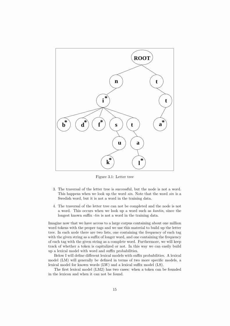
These probabilities should have values that reflect the relative share of eachsuffix in the class of nouns. If we use an appropriate data model for representingwords and their probabilities, we should be able to look up suffix probabilitiesfor unknown words efficiently by the same operation that is used for the lexicalprobability of known words. For this reason, I will use a trie, or letter tree, torepresent the lexical model [1]. Moreover, I will insert words backwards in orderto facilitate the retrieval of suffixes.

Figure 3.1 shows an example of a letter tree with the Swedish words in, bin,din, fin, kusin, latin and att inserted in the letter tree backwards. If a nodehas an asterisk it means that the path from the node to the child of root is aword, given the small amount of training data enumerated above. When wewant to use the letter tree to find a token we must traverse the trees startingfrom the end of the word. We can define four cases when searching for a tokenin a lexicon organized as a backwards letter tree:

1. The traversal of the letter tree is successful according to the token andthe final node in the traversal is a word. This means that the token is aknown word. This happens, for example, when we look up the words bin,att and kusin in the tree in figure 3.1.

2. The traversal of the letter tree can not be completed, but the node wherethe traversal stops is a word. This happens in our example when look upthe words such as rabbin and kabin, since bin is a word in the trainingdata.

1Strictly speaking stems may be decomposed into roots, but this complication is ignored.

14

a

*

u

l

ROOT

b d f s t* *

n

i*

a*

t

t

k* *

Figure 3.1: Letter tree

3. The traversal of the letter tree is successful, but the node is not a word.This happens when we look up the word sin. Note that the word sin is aSwedish word, but it is not a word in the training data.

4. The traversal of the letter tree can not be completed and the node is nota word. This occurs when we look up a word such as kantin, since thelongest known suffix -tin is not a word in the training data.

Imagine now that we have access to a large corpus containing about one millionword tokens with the proper tags and we use this material to build up the lettertree. In each node there are two lists, one containing the frequency of each tagwith the given string as a suffix of longer word, and one containing the frequencyof each tag with the given string as a complete word. Furthermore, we will keeptrack of whether a token is capitalized or not. In this way we can easily buildup a lexical model with word and suffix probabilities.

Below I will define different lexical models with suffix probabilities. A lexicalmodel (LM) will generally be defined in terms of two more specific models, alexical model for known words (LW) and a lexical suffix model (LS).

The first lexical model (LM2) has two cases: when a token can be foundedin the lexicon and when it can not be found.

15

PLW2(w|t) =PLM1(w, t)PCM1(t)

If the token is known we simple use the same probability as we did in thebaseline model. This means that a token must be traversed successfully in theletter tree and the final node in the traversal must be a word; otherwise thetoken is unknown. If the token is unknown we use the longest known suffix s tocalculate the suffix probability:

PLS2(s, t) =C(s, t) + k

N + k|W |

PLS2(s|t) =PLS2(s, t)PCM1(t)

PLM2(w|t) ={PLW2(w|t) if w ∈WPLS2(s|t) otherwise

In the general suffix model I use the longest possible suffix s which can be foundin the letter tree.

The lexical models (LM3-LM6) are variants of the lexical model (LM2),where I will reuse the definitions of PLW2(w|t) and PLS2(s|t) if possible. Theonly difference between lexical models (LM2) and (LM3) is that a token couldalso use probability PLW2(s|t) if the longest suffix s is a known word. Thismeans that the final node in the traversal of the token is a word, otherwise thetoken is unknown.

PLM3(w|t) =

PLW2(w|t) if w ∈WPLW2(s|t) if w /∈W ∧ s ∈WPLS2(s|t) otherwise

In the lexical baseline model we eliminated closed classes as candidate parts-of-speech for unknown words. With the lexical model (LM4) we will see if theperformance increases when we eliminate closed classes using the same set ofopen classes OC:

PLM4(w|t) =

PLW2(w|t) if w ∈WPLS2(s|t) if w /∈W ∧ t ∈ OC0 otherwise

Usually a Swedish sentence starts with a capitalized word. With the lexicalmodel (LM5) I will define a model which takes advantage of this knowledge. Ifa token comes after a delimiter in the set D = ., !, ? occurrences we summarizethe frequencies of capitalized and non-capitalized occurrences when calculatingthe probabilities. We can define the model PLM5 as follows:

PLW5(w, t) =C(wlower, t) + C(wupper, t) + k

N + k|W |

PLW5(w|t) =PLW5(w, t)PCM1(t)

PLS5(s, t) =C(slower, t) + C(supper, t) + k

N + k|W |

16

PLS5(s|t) =PLS5(s, t)PCM1(t)

where wlower is the same as w except (possibly) that the first letter is in low-ercase, and wupper is the same as w except (possibly) that the first letter is inuppercase. The notation slower and supper is used analogously except that “thefirst letter” is the first letter not of the suffix but of the complete word of whichit is a part.

PLM5(w|t) =

PLW2(w|t) if w ∈W ∧ wi−1 /∈ DPLS2(s|t) if w /∈W ∧ wi−1 /∈ DPLW5(w|t) if w ∈W ∧ wi−1 ∈ DPLS5(s|t) if w /∈W ∧ wi−1 ∈ D

Finally, we will see if a different maximum suffix length can improve the per-formance of the tagger. If the token is known in the lexicon the probabilityPLW2(w|t) will be used, but when the token is unknown a different suffix modelwill be used.

PLM6(w|t) ={PLW2(w|t) if w ∈WPLS2(sL|t) otherwise

The suffix sL is longest possible suffix but not longer than L. This means thatif a token can not be traversed completely in the letter tree or the final node ofthe token is not a known word and the path from the root’s child is longer thanL, then we use the suffix with path length L.

3.3 Contextual models

In section 2.3.2, we saw how the contextual probabilities can be computed withrelative frequencies in different n-class models. Without any smoothing we canassume that the tagger will not perform well because there are probably zerofrequencies in the training data. For the baseline contextual model (CM1) insection 3.1 we defined different n-class models with additive smoothing.

The contextual model (CM2) and (CM3) instead use linear interpolation, seesection 2.4.2. First, linear interpolation is computed with relative frequencies(CM2).

PCM2(ti|ti−1) = λ1C(ti−1)N

+ λ2C(ti−1, ti)C(ti−1)

PCM2(ti|ti−2, ti−1) = λ1C(ti−1)N

+ λ2C(ti−1, ti)C(ti−1)

+ λ3C(ti−2, ti−1, ti)C(ti−2, ti−1)

Secondly, linear interpolation is computed with additive smoothing (CM3). Ireuse the definition of unigram PCM1(ti), bigram PCM1(ti|ti−1) and trigramPCM1(ti|ti−2, ti−1) in the baseline model (CM1).

PCM2(ti|ti−1) = λ1PCM1(ti) + λ2PCM1(ti|ti−1)

PCM3(ti|ti−2, ti−1) = λ1PCM1(ti) + λ2PCM1(ti|ti−1) + λ3PCM1(ti|ti−2, ti−1)

The optimization parameters λ1, λ2 and λ3 are different in the bigram and tri-gram model, but I will use the same optimization parameters for the model

17

computed with relative frequencies (CM2) and with additive smoothing (CM3).I will determine the optimization parameters by simply experiment with differ-ent values and use the value which gives the highest accuracy.

18

Chapter 4

Implementation

Now we have the contextual and lexical models defined in chapter 3. Before anempirical evaluation of the models can be done we need a program which imple-ments the models in an efficient way. In this chapter I will present the generaldesign and the most important implementation issues. In chapter 1 I formu-lated primary and secondary goals about what the tagger should accomplish.In section 4.1 discuss shortly how these goals are accomplished.

4.1 Preliminaries

The obvious goal for a part-of-speech tagger is to tag as many words correctlyas possible. By using well-known theory about probabilistic tagging and thedefined models in the previous chapter, we can hopefully get a fairly high accu-racy rate. Chapter 5 is dedicated to a discussion and evaluation of the models,so in this chapter I will only explain how the models implemented.

Another important goal are efficiency regarding time and space consumption.The first step to better performance is to improve the algorithm. I have tried toeliminate unnecessary loops, move out code from loops and reduce the numberof iterations. I have gained the must of the improvements with a sharpenedalgorithm. This work is described in section 4.4. It is also important to optimizethe code using a good compiler with all available optimization features.

If an application is not user friendly it may not be used. The target user ofthe application is user with knowledge about programming who knows how tocompile a program. I have created a console-based user interface. The applica-tion can be executed with different options. To handle these options the useronly has to change a text file before executing the application. This is describedin section 4.7. In the future I will maybe do a graphical user interface as aweb-based application.

Hopefully the tagger will be used in the future and one of the secondary de-sign goals was to design and implement the tagger in such a way that it can beextended and changed easily. I have created an application with exchangeablemodules so that new module can be added in the future e.g. a new tokenizer.Figure 4.1 gives a schematic view of the MALT tagger. The ellipses are pro-grams, the boxes are modules in the programs and to the right there is a logicalview of secondary storage. Some of the smaller boxes corresponds to implemen-

19

Segmenting Viterbi

Tagger

Trie Charset

Lexical model

Unigram Bigram Trigram

Contextual modelLexical model

Probabilites/Frequencies

Contextual model

Probabilites/Frequencies

Disk

CorpusTraining data

Test data

Untagged text

Tagged text

Output

Tagset

Action Option

Tokenizer Tagset

Option file

Create tagset

Tag Analyser

MALT tagger Tagging

Training

Utility

Figure 4.1: Schematic view of the part-of-speech tagger

tation units, but not all of them. The arrows between the shapes indicate ainteraction.

As already mentioned MALT tagger can be executed in different ways byediting an option file. The option and action modules handle how the taggershould be executed. The two main uses of the tagger are training and tagging.

The training phase builds the contextual and lexical models given a corpus oftraining data and is implemented in the module with the same name. The lexicalmodel uses a trie data structure to store suffixes and words. The contextualmodel uses n-dimensional arrays depending on which n-class model the array isintended for. The contextual and lexical models are stored in separate files inthe secondary storage after training.

The tagging phase loads contextual and lexical models from file and then thetagger module takes over. The tagger module have two main tasks, to divide theuntagged text into chunks and then tag each chunk using the Viterbi algorithm.

The utility module contains auxiliary functions for the two main phases.The tagset unit helps the program convert between the internal representationof the tagset and the currently used tagset. The tokenizer unit helps the programto read tagged and untagged text such as different corpora or ordinary text inspecial formats. The tag analyzer is an auxiliary program which generate tagsetfiles with the internal representation of the tagset from different corpora.

Which programming language should I use? It is not easy to choose pro-gramming language from a scientific point of view. Here are some of the issuesinvolved:

• Which languages do you know?

• What is the nature of your problem?

• Does the language have many resources such as an Application Program-ming Interface (API)?

• Are there good compiler which generate fast executable code?

20

• Is the language platform independent?

• Do you need to control low-level features of the operating system?

I have chosen the C programming language because of the nature of the problem.We need a language that can produce efficient executable code and supplied witha good compiler. I have used the GNU C Compiler with many optimizationfeatures. The compiler is available for different operating system such as Unix,Linux and Microsoft Windows. C does not have good support with respectto predefined data structures and algorithms. The programming language Javahas quite good support of predefined data structures, but some of the structuresused in this implementation are not included. I think that the best solution is toimplement the time consuming parts in C, and by using a Java Native Interface(JNI) connect a Java application to the C implementation. The native interfacewill not be included in this thesis.

4.2 Lexical model

The lexical model contains a list of possible tags for each word and in some casesfor each suffix with respect to the training data. A probability is assigned toevery possible tag in relation to the word. In chapter 3 I defined different ways tocalculate the probability and I also extended the model with suffix probabilitiesP (s|t). This means that not only words of occurring with different tags have alist of possible tags but also every suffix of a word has a probability. A lettertree can be used to represent the suffix and word tree and the data structure ofthis representation is called a trie.

The trie data structure is a tree structure often used to represent collectionsof words and in this application also collections of suffixes. Each node in thetrie contains a set of characters which points to the next character in the word.This structure makes it quite fast to look up words in a dictionary since the timeto find a word is proportional to the length of the word. The benefit of thisdata structure is that it is very fast to find, insert and delete words. The majordisadvantage is that the trie consumes enormous amounts of memory. If we wantto represent every combination in an 8-bit ASCII code the amount of memorywill grow exponentially as the tree gets deeper. If every node contains 1028 bytesand the depth of the trie is 3 we need about 17 GBytes of memory. Fortunatelywe do not have to represent all combinations but only a small subset, becauseof two things. First of all, the trie will be sparse since most possible strings usenot found in the training data. Secondly, we can reduce the character set to asubset of the ASCII codes. To reduce the character set a function is needed tomap characters to the data structure in the node that contains links to the nextlevel in the trie. This is done in the module charset shown in figure 4.1. Forinstance, we can map an uppercase letter to the corresponding lowercase letterand let the node separate them. We also have one dummy character to whichwe map many of ASCII codes which are not human readable and not likely tooccur in the training material.

Figure 4.2 shows how the trie node is structured. Each node contains acharacter, a boolean variable assigned the value true if the sequence of charactersending in this node is a word and an array of pointers to the next level in thetrie. The structure also contains two pointers which each points to a linked

21

...

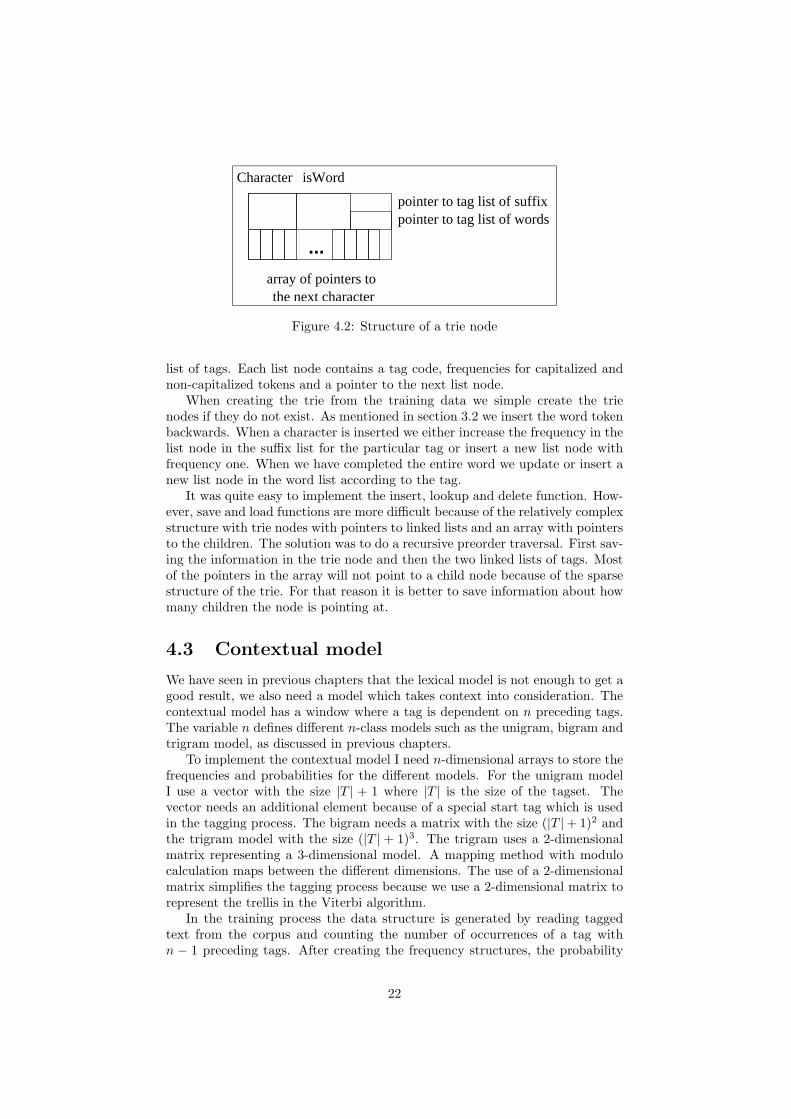
array of pointers to the next character

Character isWord

pointer to tag list of wordspointer to tag list of suffix

Figure 4.2: Structure of a trie node

list of tags. Each list node contains a tag code, frequencies for capitalized andnon-capitalized tokens and a pointer to the next list node.

When creating the trie from the training data we simple create the trienodes if they do not exist. As mentioned in section 3.2 we insert the word tokenbackwards. When a character is inserted we either increase the frequency in thelist node in the suffix list for the particular tag or insert a new list node withfrequency one. When we have completed the entire word we update or insert anew list node in the word list according to the tag.

It was quite easy to implement the insert, lookup and delete function. How-ever, save and load functions are more difficult because of the relatively complexstructure with trie nodes with pointers to linked lists and an array with pointersto the children. The solution was to do a recursive preorder traversal. First sav-ing the information in the trie node and then the two linked lists of tags. Mostof the pointers in the array will not point to a child node because of the sparsestructure of the trie. For that reason it is better to save information about howmany children the node is pointing at.

4.3 Contextual model

We have seen in previous chapters that the lexical model is not enough to get agood result, we also need a model which takes context into consideration. Thecontextual model has a window where a tag is dependent on n preceding tags.The variable n defines different n-class models such as the unigram, bigram andtrigram model, as discussed in previous chapters.

To implement the contextual model I need n-dimensional arrays to store thefrequencies and probabilities for the different models. For the unigram modelI use a vector with the size |T | + 1 where |T | is the size of the tagset. Thevector needs an additional element because of a special start tag which is usedin the tagging process. The bigram needs a matrix with the size (|T |+ 1)2 andthe trigram model with the size (|T | + 1)3. The trigram uses a 2-dimensionalmatrix representing a 3-dimensional model. A mapping method with modulocalculation maps between the different dimensions. The use of a 2-dimensionalmatrix simplifies the tagging process because we use a 2-dimensional matrix torepresent the trellis in the Viterbi algorithm.

In the training process the data structure is generated by reading taggedtext from the corpus and counting the number of occurrences of a tag withn − 1 preceding tags. After creating the frequency structures, the probability

22

structures are calculated according to the model used. The result of the delim-iter tag is copied to the first and the special start tag because the segmentationof the text in the tagging process assumes that the model starts with a newsentence, see section 4.4. Finally, the frequency and probability structures arestored in separate files. An internal representation of the tagset is used, eachtag being represented by an integer value called tag code. This tag code is usedwhen accessing data in the different structures.

4.4 Segmentation and Viterbi

The previous sections have mostly concerned the implementation of the trainingprocess of the contextual and the lexical models. They are of no use if we cannot use them to tag a Swedish text and in this section we will discuss theimplementation of the tagging process. First the tagger most be initialized withmodels by loading them from the secondary storage. The next step is to tag anuntagged text or as in the empirical evaluation a tagged corpus.

Suppose we have about 100000 untagged words and a tagset with 150 tagsand use the trigram model and every probability needs 4 bytes of memoryspace. This will result in a huge matrix when using the Viterbi algorithm:4(100000(150 + 1)2) ≈ 9 GBytes. We need to segment the untagged text intosmaller chunks and then run the Viterbi algorithm on each chunk.

An easy approach is to cut the text into equally sized pieces except for thelast piece. Unfortunately this will result in decreased accuracy because cuttingcan occur in the middle of a sentence and we then lose information about con-textual dependencies. A more complex solution is to always cut between twounambiguous words. A disadvantage of this approach is that we need to keeptrack of unambiguous word or determine it during run-time which is memoryand time consuming. If we use the trigram model it will be even more compli-cated because we need to keep track of three unambiguous words, since the twoprevious words need to be unambiguous.

My approach is to use sentence delimiters such as period and question markas markers for a cutting point. Usually there are no contextual dependencies re-garding parts-of-speech over the sentence boundary. The segmentation methoduses an interval between cutmin and cutmax where the sentence delimiter canbe used for cutting the text. We need to set a maximum size because we needto allocate enough memory for the trellis matrix in advance.

Now we have a mechanism to divide the text into smaller chunks. A chunkrefers to a word sequence which will be tagged separately. In section 2.5 we haveseen the Viterbi algorithm which helps the tagger to find the most probable paththrough the Hidden Markov Model.

I have used the following version of the Viterbi algorithm when tagging witha bigram model [9]:

23

1. Create1.1 A path probability matrix trellis[|T |+ 1, |S|+ 1]1.2 A backpointer matrix backpointer[|T |+ 1, |S|+ 1]

2. For every i, j trellis[i, j]← 0.03. trellis[0, 0]← 1.04. For each word s in sequence S do

4.1 For each state c in set C do4.1.1 For each previous state p in set P do

4.1.1.1 newscore← trellis[p, s− 1] ∗ lexical[s]∗contextual[p, s]

4.1.1.2 if (newscore > trellis[c, s]) then4.1.1.2.1 trellis[c, s]← newscore4.1.1.2.1 backpointer[c, s]← c

5. back ← backpointer[1, |S|]6. max← trellis[1, |S|]7. For each state t in T do

7.1 if (max < trellis[t, |S|] then7.1.1 back ← backpointer[t, |S|]

8. For each state s from |S| − 1 to 1 do8.1 Print back8.2 back ← backpointer[back, s]

Viterbi uses two matrices trellis and backpointer to complete the task, one forsaving the highest probabilities for a specific path and one for saving the actualpath. The trellis matrix needs to be initialized with zero probabilities exceptfor the starting state, which is initialized with the highest probability.

To compute the best possible path or tag sequence we need three nestedloops. The first loop reviews every symbol s in the input sequence S, whichconsists of the input sequence of tokens. For every symbol s we have to computethe highest probability for going from a previous state p to the current statec. The set C consists of all possible tags which the lexical model containsfor a particular word or suffix and the set P consists of all possible tags forthe previous word or suffix. In the innermost loop the algorithm computesa new score by multipling the previous score with the lexical and contextualprobabilities. If the new score is higher then the current score, the new scorewill be assigned as the current score. At the same time the state is saved in theback-pointer matrix to keep track of the path.

When all the columns of the trellis have been filled the algorithm uses theback-pointer matrix to find the best possible tag sequence according to thelexical and contextual model. To find the path through the back-pointer matrixthe algorithm takes the corresponding state, which has the highest score in thetrellis matrix, and then uses this state to find the tag sequence in the last loop.

In my implementation I actually use logarithms of probabilities to cope withthe problem of accuracy of floating-point values, since probabilities may becometoo small to be represented in the computer. This representation alters thealgorithm a little. For example, instead of multipling the probabilities whencomputing the new score the algorithms sum them together and the startingstate is initialized with the value 0.0 and the rest of the matrix initialized withthe value 1.0 which indicates an illegal probability.

24

When the trigram model is used the algorithm usus two preceding tags tocalculate the new score and to do so the algorithm uses one more nested loopto review the extra preceding tag.

4.5 Tokenizer

The first step in the analysis of the text input is usually the tokenization of theinput into words and punctuation. For many languages such as Swedish thisproblem is fairly easy in that one can to a first approximation assume that wordboundaries consist of white space or punctuation in the input text.

I have implemented an uncomplicated tokenizer which assumes that everytoken is surrounded by white space, this also including punctuation tokens. Inthe future I may construct a more sophisticated tokenizer.

This module also includes functions for reading a line from a tokenized andtagged corpus. The tokenizer supports the format for SUC version 1, SUCversion 2 and a tab separated word/parts-of-speech corpus. A new tokenizercan easily be implemented in the tokenizer module. When using the modulewe simple call the gettoken() function and the module uses the appropriatetokenizer stated in the option file.

4.6 Tagset

One of the requirements is that the tagger should be corpus independent. Thisrequires an internal representation of the possible tags. The solution is to use aninteger to represent a tag. The tagset is stored as a hash table with a structurecontaining two strings tag (part-of-speech) and m (morpho-syntatic features).An integer tagcode is used in the rest of the program to represent the tags in thelexical and contextual model. Only when the program gets input and generatesoutput are the tag and optional m used. Optional structure items word, andfreq are not important, but it is quite good to have an example of a word. Tocreate a tagset we either create a file with the following tab-separated format:

tag m tagcode word_example freq

or use the Tag analyzer program to read a corpus and generate the tagset file.The tagset file also counts the number of occurrences of each tag. This frequencyis not used in the training or tagging process, it is only for presentation of thetagset.

4.7 Options

When executing the MALT tagger we need an easy way to vary between differentsettings. One solution could be to use of a menu where the user choose a betweenthe possible settings. The disadvantage of this approach is that it takes toomuch time to change the different parameters. Another approach is to invokethe program with different arguments. Usually this approach is good, but theproblem is that there are to many options. My solution is to have an optionfile which the user can manipulate. The option file is loaded when the programstarts by entering the path to the option file as an argument:

25

% malttagger -of==/path/filename

In the option file we can choose tagset, tokenizer, test methods, contextualmodel and lexical model. We can also choose between different actions such astraining and tagging, or both.

26

Chapter 5

Evaluation

In this chapter I will present an empirical evaluation of different models fortagging Swedish text. The models are defined in chapter 3 and their implemen-tation is described in chapter 4. I will use a tagged corpus in both the trainingprocess and the test phase. In the training process I will use one part of thecorpus to create the lexical model by counting the occurrences of a word witha given part-of-speech and the contextual model by counting the occurrences ofunigrams, bigrams and trigrams. In the test phase I will use a different part ofthe corpus to test the accuracy by tagging the tokens and then checking if thetagger has assigned the correct tag.

5.1 Corpus data

The data used for the empirical evaluation come from the Stockholm-UmeaCorpus (SUC) version 2.0. This corpus is a balanced corpus of written Swedishfrom different areas such as newspaper text and fiction. The version SUC 2.0 isnot an official release. The corpus has been automatically tagged for parts-of-speech and then corrected manually [6, 10].

By processing the entire corpus I could identify that the corpus contains1, 166, 603 tokens (punctuation included). The corpus is divided into small filesof about 2500 tokens in each file. The tagset used consists of 25 basic parts-of-speech and I will call this tagset the small tagset in the evaluation. Thelarge tagset includes also morpho-syntactic features and the large tagset has153 distinct tags. The tagsets are described in appendix A and B.

5.2 Evaluation

In the empirical evaluation the Stockholm-Umea Corpus will be divided in dif-ferent ways to get as reliable results as possible. First of all I will save a smallsubset of the corpus to test the tagger when the evaluation of the different mod-els is finished. The final test will only test the best model(s) and the baselinemodel with respect to their the accuracy rate, giving an estimate of the ac-curacy when applied to unseen text. In the final test I will also evaluate thepart-of-speech tagger’s time consumption. I have chosen to use 1, 101, 483 to-kens to train the models and 65120 tokens to test the tagger in the final test. I

27

Table 5.1: Cross ValidationRound Word Known Unknown Total

types words words1 86264 103968 8852 1128202 86804 104758 7784 1125423 86980 102036 7695 1097314 86955 102440 7995 1104355 86487 101443 8682 1101256 86755 100692 8074 1087667 86948 100725 8155 1088808 86752 101213 8172 1093859 87425 100453 7527 10798010 86836 102879 7940 110819Total: 1020607 80876 1101483

randomly selected the files that should be in the training and test set, but withone restriction that there should be a good distribution over different areas oftexts.

Before the final test can be done we need to evaluate the different lexicaland contextual models and identify the best model(s). Cross-validation is atool for selection of statistical models and is a very general framework usingno special model assumptions. Cross-validation gives an estimate of a model’sgeneralization capabilities [11]. When a cross-validation is performed we dividethe data into k subsets of approximately equal size. We then train the modelk times, each time leaving out one of the subsets from training. The excludedsubset in the training is used to test the model and this will also be performedk times.

I will perform a cross-validation and the training data in the final test willbe used for the cross-validation. I have decided to use k = 10, which meansthat the data will be divided into 10 subsets. We can now define a validationround as 9 subsets for training and one subset for testing the tagger. Table 5.1shows the number of unknown and known words and the total for each testinground. I will not present the accuracy rate for each round, instead the meanwill be presented.

When evaluating the different models I will present four different accuracyrates: small tagset with bigram model, small tagset with trigram model, largetagset with bigram model and large tagset with trigram model.

5.3 Results

5.3.1 Lexical model

The lexical model estimates the probability of a word given its part-of-speechP (w|t). In section 3.2 different lexical models are defined. In this section Iwill perform an evaluation of the models and find out which model is the bestaccording to accuracy. To do the experiment we need to have a contextualmodel. The contextual models used in the experiment are PCM1(ti|ti−1) and

28

Table 5.2: Results for the baseline lexical model (LM1)Tagset/ Total Known UnknownContextual model words wordsSmall/Bigram 91.96 95.95 41.69Small/Trigram 93.60 96.09 62.19Large/Bigram 89.92 95.39 20.92Large/Trigram 88.60 93.36 28.53

PCM1(ti|ti−2, ti−1), for bigram and trigram respectively, as defined in section3.3. No changes to the contextual model will be done under the experimentwith the lexical model.

First of all we will test the baseline lexical model, which uses additivesmoothing to handle the problem with sparse data. If a token is known inthe lexicon the probability PLM1(w|t) is used and if it is unknown PLM1(wu|t)is used. The results of the experiment are shown in table 5.2.

The results for known words are quite good for the small tagset, but forthe unknown words it is really bad. The poor results are more visible for thelarge tagset, since there are more choices and not enough data to do a goodestimation. A more sophisticated smoothing method is needed.

One of the primary purposes of this thesis is to find out if a lexical modelwith suffix probabilities can be used to improve both tagging accuracy andefficiency. In section 3.2 I have defined five different lexical models with suffixprobabilities, summarized below:

• LM2 : If the token is known we simple use the probability from the baselinemodel (LM1), otherwise the longest possible suffix s is used to calculatethe suffix probability PLS2(s|t).

• LM3 : The same lexical model as (LM2) but with an important difference.The probability from the baseline is also used when the longest possiblesuffix belongs to the set of known words with respect to the training data.

• LM4 : The closed classes are eliminated when the token is unknown.

• LM5 : When a word occur sentence initially we sum the frequencies forcapitalized and non-capitalized occurrences when calculating the proba-bilities for words and suffixes.

• LM6 : When a token is unknown will this lexical model use a suffix withmaximum length L.

The results for the lexical model (LM2) is presented in table 5.3. We can see asubstantial improvement from the baseline lexical model for unknown words anda tiny improvement for the known words. The difference between the small andthe large tagset decreases for the unknown words. The lexical models (LM3-LM5) were also tested, but the differences found were very small and surelynot statistically significant. The result will not be presented here because thedifferences between (LM2) and (LM3-LM5) were only a few hundredths of apercentage.

29

Table 5.3: Results for the lexical model with suffix probabilities (LM2)Tagset/ Total Known UnknownContextual model words wordsSmall/Bigram 95.32 96.16 84.70Small/Trigram 95.29 96.18 84.13Large/Bigram 94.43 95.58 79.87Large/Trigram 92.88 93.97 79.15

Table 5.4: Results for the lexical model with suffix probabilities and maximumsuffix length L (LM6)

Tagset/ 4 5 6 7 8 No limitContextual model limitSmall/Bigram 95.11 95.22 95.30 95.31 95.32 95.32Small/Trigram 95.16 95.23 95.28 95.29 95.30 95.29Large/Bigram 94.28 94.37 94.45 94.45 94.45 94.43Large/Trigram 92.65 92.79 92.88 92.90 92.89 92.88

Another interesting experiment is to vary the maximum length of the suffix,which is defined as the lexical model (LM6). I vary the maximum length of thesuffix L from 4 to 8. In table 5.4 we can see the parameter L in the columnsand in the rightmost column we have the results from (LM2). To minimize thenumbers I have excluded the data about known and unknown words. We cansee a slight improvement with a maximum suffix length around 7, but it is nota significant improvement. The lexical model (LM6) needs at least to have amaximum suffix length greater than 4.

To summarize the results of the lexical model we can see a difference betweenthe baseline lexical model and the lexical model with suffix probabilities, whichis found to be statistically significant given clear the size of the datasets. Wecan not find any difference between the lexical models with suffix probabilities.Based on the evaluation of the lexical model I have decided to use the lexicalmodel (LM2) for the forthcoming test, since there is no visible difference be-tween the lexical models (LM2-LM6), and the lexical model (LM2) is the moststraightforward way to implement a lexical model with suffix probabilities.

5.3.2 Contextual model

In the previous chapters we have concluded based on previous work in thisarea that a lexical model is not enough to find the tag sequence for a givenstring of words. We also need information about the context where the wordis found. The contextual model is created by computing the probability ofa part-of-speech conditioned on a sequence of previous tags. In section 3.3 Idecided to use a bigram model P (ti|ti−1) and a trigram model P (ti|ti−2, ti−1).These probabilities can be computed in different ways such as with additivesmoothing (CM1), with linear interpolation with relative frequencies (CM2)and with linear interpolation with additive smoothing(CM3). In this evaluationthe lexical model will be the same as in section 5.3.1 I decided to use the lexical

30

Table 5.5: Results for the contextual model with linear interpolation of relativefrequencies (CM2)

Tagset/ Total Known UnknownContextual model words wordsSmall/Bigram 95.32 96.17 84.67Small/Trigram 95.33 96.18 84.59Large/Bigram 94.49 95.65 79.98Large/Trigram 85.45 86.57 71.29

Table 5.6: Results for the contextual model with linear interpolation of additivesmoothing (CM3)

Tagset/ Total Known UnknownContextual model words wordsSmall/Bigram 95.33 96.17 84.70Small/Trigram 95.59 96.45 84.68Large/Bigram 94.44 95.60 79.90Large/Trigram 94.77 95.91 80.34

model (LM2).One of the easiest way to calculate the probability is to use relative frequen-

cies without any smoothing methods, but this is not a good idea because of thesparse data problem. With the small tagset and bigram model maybe there willnot be any zero-frequencies and maybe the result is not too bad, but with thetrigram model there will be many zero-frequencies. A contextual model whichonly uses on relative frequencies is not reliable and will not be used.

To eliminate the problem with zero-frequencies we must use a smoothingmethod. In tables 5.2 and 5.3 I used additive smoothing for the contextualmodels (CM1). The purpose of using the more complex trigram model is tohave better accuracy rate than the bigram model, but still the results are quitepoor. Due to the lack of training data the trigrams in some cases can not beestimated properly [15].

Another smoothing method is to experiment with a linear interpolation ofthe unigram, the bigram and the trigram. Linear interpolation can maybeimprove the accuracy rates specially for the trigram model. The experimentwith linear interpolation will be done with both relative frequencies (CM2) andadditive smoothing (CM3), and the results are shown in table 5.5 and 5.6.

In an ad hoc experiment with different optimization parameters λ1, λ2 andλ3 I found that the best accuracy rate is about λ1 = 0.02 and λ2 = 0.98 for thebigram model and λ1 = 0.14, λ2 = 0.53 and λ3 = 0.33 for the trigram model.The attentive reader notes that bigram model (CM2, CM3) practically does notuse any unigram in the linear interpolation. The improvement of the bigrammodel (CM2, CM3) is negligeable. The improvement of the trigram model withthe contextual model using linear interpolation of additively smoothed n-grams(CM3) is considerable better.

The evaluation of the contextual model shows that the model with linearinterpolation as smoothing method should be used for the trigram model. How-

31

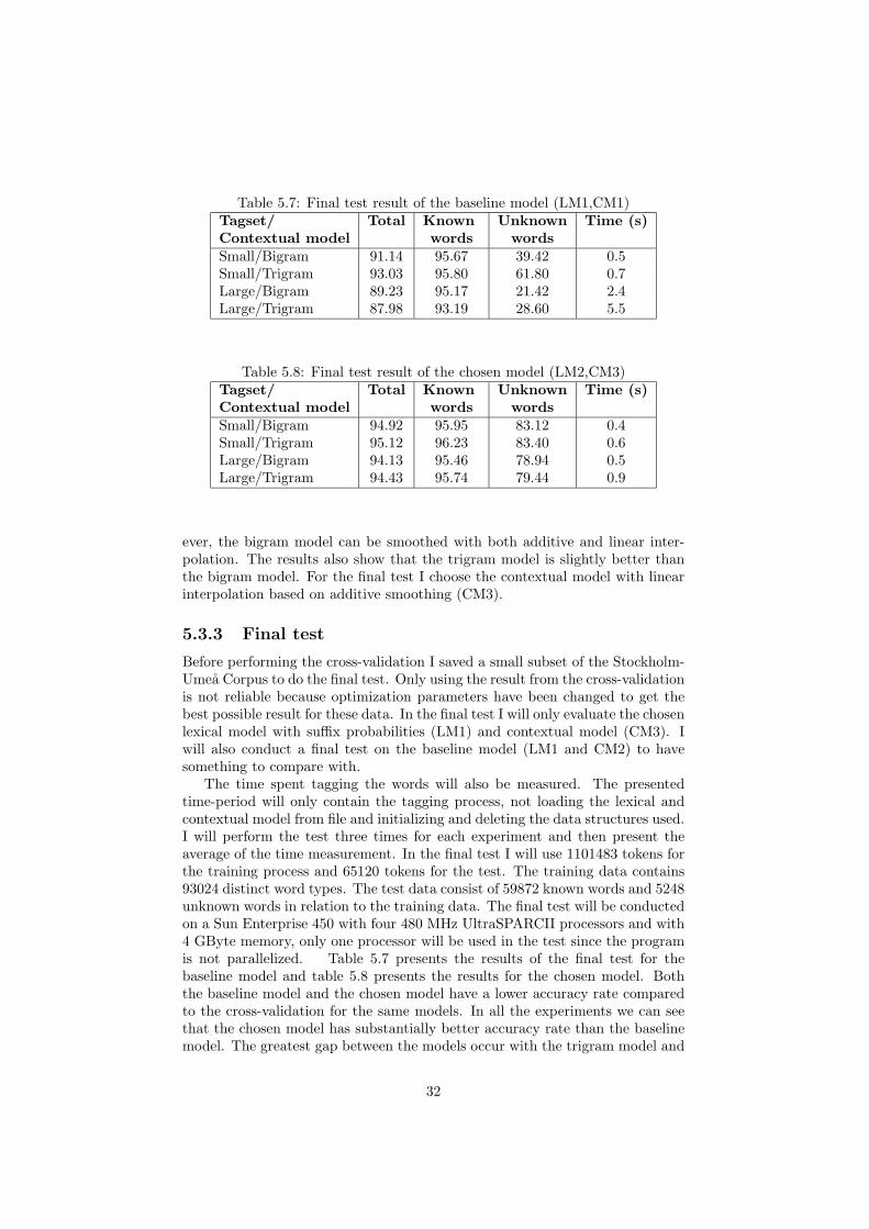
Table 5.7: Final test result of the baseline model (LM1,CM1)Tagset/ Total Known Unknown Time (s)Contextual model words wordsSmall/Bigram 91.14 95.67 39.42 0.5Small/Trigram 93.03 95.80 61.80 0.7Large/Bigram 89.23 95.17 21.42 2.4Large/Trigram 87.98 93.19 28.60 5.5

Table 5.8: Final test result of the chosen model (LM2,CM3)Tagset/ Total Known Unknown Time (s)Contextual model words wordsSmall/Bigram 94.92 95.95 83.12 0.4Small/Trigram 95.12 96.23 83.40 0.6Large/Bigram 94.13 95.46 78.94 0.5Large/Trigram 94.43 95.74 79.44 0.9

ever, the bigram model can be smoothed with both additive and linear inter-polation. The results also show that the trigram model is slightly better thanthe bigram model. For the final test I choose the contextual model with linearinterpolation based on additive smoothing (CM3).

5.3.3 Final test

Before performing the cross-validation I saved a small subset of the Stockholm-Umea Corpus to do the final test. Only using the result from the cross-validationis not reliable because optimization parameters have been changed to get thebest possible result for these data. In the final test I will only evaluate the chosenlexical model with suffix probabilities (LM1) and contextual model (CM3). Iwill also conduct a final test on the baseline model (LM1 and CM2) to havesomething to compare with.

The time spent tagging the words will also be measured. The presentedtime-period will only contain the tagging process, not loading the lexical andcontextual model from file and initializing and deleting the data structures used.I will perform the test three times for each experiment and then present theaverage of the time measurement. In the final test I will use 1101483 tokens forthe training process and 65120 tokens for the test. The training data contains93024 distinct word types. The test data consist of 59872 known words and 5248unknown words in relation to the training data. The final test will be conductedon a Sun Enterprise 450 with four 480 MHz UltraSPARCII processors and with4 GByte memory, only one processor will be used in the test since the programis not parallelized. Table 5.7 presents the results of the final test for thebaseline model and table 5.8 presents the results for the chosen model. Boththe baseline model and the chosen model have a lower accuracy rate comparedto the cross-validation for the same models. In all the experiments we can seethat the chosen model has substantially better accuracy rate than the baselinemodel. The greatest gap between the models occur with the trigram model and

32

the large tagset and this is quite natural due to the sparse data problem in thismodel. The time measurements show that the chosen model have a considerablybetter performance than the baseline, especially when the large tagset is used.

5.4 Discussion

The main result concerning the choice of lexical model is that the lexical modelwith suffix probabilities outperforms the baseline model with respect to thedata at hand. If we want to use a lexical model without suffix probabilities weneed a more sophisticated smoothing model. However, with the lexical modelwith suffix probabilities we eliminate the need for a sophisticated smoothingmodel. It seems to be enough with additive smoothing to obtain good accuracy.Moreover, in the baseline model we need to keep track of the open classes ofparts-of-speech, which increases the number of states to be calculated in thetagging process. In one of the experiments with the lexical model with suffixprobabilities I used a closed class elimination method, but the accuracy ratewas not improved. Thus, a lexical model with suffix probabilities seems toeliminate the need for such a method as well. Another interesting result wasthat the special treatment of tokens occurring at the start of a sentence didnot improve the performance of the tagger. Maybe a more complex methodcould improve the accuracy rate by taking into account other dependencies atthe start of a sentence, but it is hard to define a model which does not decreasethe accuracy for other words. My results almost confirm the results whichCarlberger & Kann [3] got concerning the maximum suffix length. They didnot get any improvement with a maximum suffix length of more than 5 letters.In my experiment I did get a slight improvement with 6 letters, but the increasein accuracy rate was not significantly better than for 5 letters.

Comparing my results with others is rather difficult, because of differenttraining data, tagsets and empirical methods. Nivre [15] has shown that Good-Turing estimation for the lexical model outperforms the additive smoothingespecially for unknown words. However, with lexical additive smoothing incombination with a lexical model with suffix probabilities the results are bet-ter than the results obtained by Nivre (small tagset 94.82% and large tagset91.46%) [15]. Especially for the large tagset the result 94.43% is substantiallybetter. The GRANSKA tagger created by Carlberger & Kann uses 140 tags,incorporates Svenska Akademiens ordlista (SAOL) and in some cases considera token as consisting of two or more words. They reports a tagging accuracy of96.4% [3].

One question we can ask ourselves, is whether the results would be even bet-ter with a combination of Good-Turing and a suffix model, but this experimentis beyond this thesis. Probably the answer is that the results would be slightlyimproved, but I do not think that any major difference will be detected.

Concerning the contextual model, we have seen that the linear interpola-tion based on additive smoothing of n-grams outperforms the simple additivesmoothing when we have a problem with sparse data, which is the case in thetrigram model especially with a large tagset. Nivre [15] has shown that withrespect to the data at hand both additive smoothing and back-off smoothing isbetter than Good-Turing estimation. My results indicate that linear interpola-tion based on additive smoothing of n-grams outperforms additive smoothing,

33

hence also the other methods.A great advantage of using a lexical model with suffix probabilities is that

a letter tree can be used to store both suffixes and words which speeds up thetagging. When an unknown word occurs we simply use the suffix probabilities,which means that the lookup of unknown words is fast (in fact faster than ifthe word had been known). Moreover the use of suffixes reduces the numberof possible tags for each word, which also improves efficiency. The performanceregarding time consumption improves dramatically when tagging with the largetagset and the trigram contextual model compared to the baseline model, whichhas to consider every open class as a candidate tag for an unknown word. Thetime difference when tagging around 65000 words with the small and large tagsetis very small with the bigram model. With the trigram model the difference isslightly larger but still surprisingly low.

In section 2.5 we noticed that the Viterbi algorithm is linear in the numberof words to be tagged, but quadratic in the number of states. The suffix modelreduces the number of states considered compared to the baseline model whichspeeds up the tagger. In addition, it makes lookup of lexical probabilities veryfast.

34

Chapter 6

Conclusion

The most important conclusion from this master’s thesis is that the lexical modelwith suffix probabilities improves the tagging of Swedish text in two differentways. First, it improves the tagging of unknown words dramatically comparedto a simple additive smoothing, and a slight improvement can also be detectedwhen comparing the result with a more sophisticated smoothing method suchas Good-Turing. Secondly, it improves efficiency since suffixes and words arestored in same structure which speeds up lexical lookup. The time complexity oflexical lookup is linear according to the length of the word or suffix. The modelalso speeds up the process of tagging, since the number of states consideredwhen finding the optimal path through the Hidden-Markov model decreases.

Using suffix analysis to improve the tagging of unknown words has been usedin several previous studies [16, 3]. However, in this thesis I have shown thatintegrating the word and suffix model using an appropriate data structure notonly increases accuracy but also efficiency.

The goal of this master’s thesis was to define tagging models and implementthese models in such a way that the tagger could accomplish an accuracy ratearound 95 percent for the Stockholm-Umea corpus with both the small tagsetand the large tagset. Although the final results with the large tagset are slightlybelow 95 percent the results indicate that this goal can be achieved with a lexicalmodel using suffix probabilities and a contextual model with linear interpolationbased on additive smoothing of n-grams. Another goal was to accomplish thisin an efficient manner, meaning that the tagger should tag 20000 tokens in asecond. In the end, the tagger tags around 70000 tokens per second on a SunEnterprise 450 with four 480 MHz UltraSPARCII processors and with 4 GBytememory, using only one processor in the test. Although it is hard to compareactual running time in a fair manner, since the test conditions are differentfrom time to time and from machine to machine, we may compare this withCarlberger & Kann [3] who reports a tagging rate of 14000 words per secondson a Sun Sparcstation 10.

The MALT tagger cannot yet be considered as a professional part-of-speechtagger. First of all, the tagger needs a better tokenizer, either by incorporatingan existing tokenizer or by implementing more sophisticated one. To improvethe tagging accuracy we need to do more experiments with both the lexical andthe contextual model. Another important aspect is to develop an interface thatother applications can use to communicate with the tagger.

35

Bibliography

[1] A. V. Aho and J. D. Ullman. Foundations of Computer Science. ComputerScience Press, 1992.

[2] E. Brill. Part-of-speech tagging. In R. Dale, H. Moisl, and H. Somers,editors, Handbook of Natural Language Processing, pages 403–414. MarcelDekker, 2000.

[3] J. Carlberger and V. Kann. Implementing an efficient part-of-speech tagger.Software — Practice and Experience, 29(9):815–832, 1999.

[4] S. F. Chen and J. Goodman. An empirical study of smoothing techniquesfor language modeling. In Proceedings of the Thirty-Fourth Annual Meetingof the Association for Computational Linguistics, 1996.

[5] T. H. Cormen, C. E. Leiserson, and R. L. Rivest. Introduction to Algo-rithms. The Massachusetts Institute of Technology, 1990.

[6] E. Ejerhed, G. Kallgren, O. Wennstedt, and M. Astrom. The linguisticannotation system of the Stockholm-Umea corpus project. Technical Re-port 33, University of Umea: Department of Linguistics, 1992.

[7] W.A. Gale and G. Sampson. Good-Turing frequency estimation withouttears. Journal of Quantitative Linguistics, 2:217–237, 1995.

[8] L. Gronqvist and M. Gunnarsson. A method for finding word clusters inspoken language. In Proceedings for Corpus Linguistics 2003 conference.UCREL, Lancaster, March 2003.

[9] D. Jurafsky and J. H. Martin. Speech and Language Processing. Prentice-Hall, 2000.

[10] G. Kallgren. Documentation of the Stockholm Umea Corpus. Technicalreport, University of Umea: Department of Linguistics, 1998.

[11] F. Leisch, K. Hornik, and L. C. Jain. Nn classifiers: Reducing the com-putational cost of cross-validation by active pattern selection. In 2nd NewZealand Two-Stream International Conference on Artificial Neural Net-works and Expert Systems (ANNES ’95), pages 91–95, 1995.

[12] C. D. Manning and H. Schutze. Foundations of Statistical Natural LanguageProcessing. MIT Press, 1999.

36

[13] T. McEnery and A. Wilson. Corpus Linguistics. Edinburgh UniversityPress, 1996.

[14] B. Merialdo. Tagging English text with a probabilistic model. Computa-tional Linguistics, 20:155–171, 1994.

[15] J. Nivre. Sparse data and smoothing in statistical part-of-speech tagging.Journal of Quantitative Linguistic, 7:1–17, 2000.

[16] C. Samuelsson. Morphological tagging based entirely on Bayesian inference.In NODALIDA’93. Proceeding of the ’9:e Nordiska Datalingvistikdagarna’,pages 225–238, 1994.

[17] A. J. Viterbi. Error bounds for convolutional codes and an asymptoticallyoptimal decoding algorithm. IEEE Transactions on Information Theory,13:260–269, 1967.

37

Appendix A

The SUC small tagset

Tag Part-of-Speech Tag code ExampleAB Adverb 7 inteDT Determiner 9 enHA Wh adverb 13 narHD Wh determiner 24 vilkaHP Wh pronoun 15 vadHS Wh possessive 25 varsIE Infinitive marker 19 attIN Interjection 23 jaJJ Adjective 8 mycketKN Conjunction 5 ochMAD Delimiter 4 .MID Delimiter 10 -NN Noun 1 SmygrustningPAD Delimiter 18 ”PC Participle 12 anseddaPL Particle 17 underPM Proper name 3 MATSPN Pronoun 11 enPP Preposition 2 avPS Possessive 20 sinaRG Cardinal numeral 21 tvaRO Ordinal numberal 22 forstaSN Subjunction 14 attUO Foreign word 16 thinktankVB Verb 6 har

38

Appendix B

The SUC large tagset

This table is taken from the documentation of the Stockholm Umea Corpus [10].

Feature Value Legend Parts-of-speechwhere feature applies

Gender UTR Uter (common) DT, HD, HP, JJ, NN,PC, PN, PS, (RG, RO)

NEU NeuterMAS Masculine

Number SIN Singular DT, HD, HP, JJ, NN, PC,PN, PS, (RG, RO)

PLU PluralDefiniteness IND Indefinite DT, (HD, HP, HS), JJ,

NN, PC, PN, (PS, RG, RO)DEF Definite

Case NOM Nominative JJ, NN, PC, PM, (RG, RO)GEN Genitive

Tense PRS Present VBPRT PreteriteSUP SupinumINF Infinite

Voice AKT ActiveSFO S-form

Mood KON SubjunctiveParticiple form PRS Present PC

PRF PerfectDegree POS Positive (AB), JJ

KOM ComparativeSUV Superlative

Pronoun form SUB Subject form PNOBJ Object formSMS Compound All parts-of-speech

39

Tag Tag code ExampleAB 11 inteAB AN 90 klAB KOM 29 oftareAB POS 31 fullkomligtAB SMS 124 upp-AB SUV 53 framstDT AN 153 dDT MAS SIN DEF 130 DenneDT MAS SIN IND 129 sammeDT NEU SIN DEF 22 detDT NEU SIN IND 56 ettDT NEU SIN IND/DEF 106 alltDT UTR SIN DEF 41 denDT UTR SIN IND 16 enDT UTR SIN IND/DEF 110 allDT UTR/NEU PLU DEF 20 deDT UTR/NEU PLU IND 85 NagraDT UTR/NEU PLU IND/DEF 66 allaDT UTR/NEU SIN DEF 131 varderaDT UTR/NEU SIN IND 70 VarjeDT UTR/NEU SIN/PLU IND 75 sammaHA 25 narHD NEU SIN IND 125 VilketHD UTR SIN IND 105 vilkenHD UTR/NEU PLU IND 104 vilkaHP - - - 36 somHP NEU SIN IND 35 vadHP NEU SIN IND SMS 149 vad-HP UTR SIN IND 108 VemHP UTR/NEU PLU IND 92 vilkaHS DEF 107 varsIE 48 attIN 103 jaJJ AN 111 tfJJ KOM UTR/NEU SIN/PLU IND/DEF GEN 127 svagaresJJ KOM UTR/NEU SIN/PLU IND/DEF NOM 50 senareJJ KOM UTR/NEU SIN/PLU IND/DEF SMS 140 aldre-JJ POS MAS SIN DEF GEN 138 intellektuellesJJ POS MAS SIN DEF NOM 67 irakiskeJJ POS NEU SIN IND GEN 151 angelagetsJJ POS NEU SIN IND NOM 12 mycketJJ POS NEU SIN IND/DEF NOM 117 egetJJ POS UTR - - SMS 123 lag-JJ POS UTR SIN IND GEN 119 anhorigsJJ POS UTR SIN IND NOM 24 optimistiskJJ POS UTR SIN IND/DEF NOM 82 egenJJ POS UTR/NEU - - SMS 132 utrikes-

40

Tag Tag code ExampleJJ POS UTR/NEU PLU IND NOM 84 fleraJJ POS UTR/NEU PLU IND/DEF GEN 99 dodasJJ POS UTR/NEU PLU IND/DEF NOM 21 politiskaJJ POS UTR/NEU SIN DEF GEN 134 flirtigasJJ POS UTR/NEU SIN DEF NOM 13 GamlaJJ POS UTR/NEU SIN/PLU IND NOM 133 rattJJ POS UTR/NEU SIN/PLU IND/DEF NOM 63 langtgaendeJJ SUV MAS SIN DEF GEN 152 aldstesJJ SUV MAS SIN DEF NOM 122 sisteJJ SUV UTR/NEU PLU DEF NOM 93 flestaJJ SUV UTR/NEU PLU IND NOM 139 FlestJJ SUV UTR/NEU SIN/PLU DEF NOM 47 bastaJJ SUV UTR/NEU SIN/PLU IND NOM 109 starkastKN 9 ochKN AN 120 &MAD 6 .MID 18 -NN - - - - 57 fjolNN - - - SMS 142 styr-NN AN 95 krNN NEU - - - 141 ordaNN NEU - - SMS 76 hotell-NN NEU PLU DEF GEN 94 LandstingensNN NEU PLU DEF NOM 8 stormaktsblockenNN NEU PLU IND GEN 89 arsNN NEU PLU IND NOM 3 raketvapenNN NEU SIN DEF GEN 44 omradetsNN NEU SIN DEF NOM 14 testamentetNN NEU SIN IND GEN 102 budsNN NEU SIN IND NOM 28 tovaderNN UTR - - - 114 dagsNN UTR - - SMS 96 planerings-NN UTR PLU DEF GEN 62 irakiernasNN UTR PLU DEF NOM 17 konflikternaNN UTR PLU IND GEN 74 nationersNN UTR PLU IND NOM 27 missilerNN UTR SIN DEF GEN 60 vastvarldensNN UTR SIN DEF NOM 7 AvspanningenNN UTR SIN IND GEN 88 fredagsNN UTR SIN IND NOM 1 SmygrustningPAD 43 ”PC AN 116 tfPC PRF MAS SIN DEF GEN 113 knivhuggnesPC PRF MAS SIN DEF NOM 101 utsandePC PRF NEU SIN IND NOM 71 kantPC PRF UTR SIN IND GEN 145 uppsagdsPC PRF UTR SIN IND NOM 38 anseddPC PRF UTR/NEU PLU IND/DEF GEN 81 deporterades

41

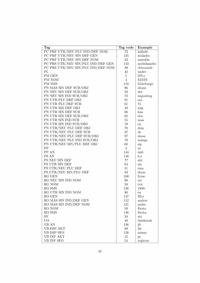
Tag Tag code ExamplePC PRF UTR/NEU PLU IND/DEF NOM 73 kalladePC PRF UTR/NEU SIN DEF GEN 135 ataladesPC PRF UTR/NEU SIN DEF NOM 23 anseddaPC PRS UTR/NEU SIN/PLU IND/DEF GEN 143 asylsokandesPC PRS UTR/NEU SIN/PLU IND/DEF NOM 39 oberoendePL 42 underPM GEN 5 DN:sPM NOM 4 MATSPM SMS 118 Goteborgs-PN MAS SIN DEF SUB/OBJ 86 dennePN NEU SIN DEF SUB/OBJ 32 detPN NEU SIN IND SUB/OBJ 72 nagontingPN UTR PLU DEF OBJ 91 ossPN UTR PLU DEF SUB 61 ViPN UTR SIN DEF OBJ 33 migPN UTR SIN DEF SUB 26 hanPN UTR SIN DEF SUB/OBJ 65 denPN UTR SIN IND SUB 55 manPN UTR SIN IND SUB/OBJ 19 enPN UTR/NEU PLU DEF OBJ 78 demPN UTR/NEU PLU DEF SUB 37 dePN UTR/NEU PLU DEF SUB/OBJ 97 dessaPN UTR/NEU PLU IND SUB/OBJ 79 mangaPN UTR/NEU SIN/PLU DEF OBJ 68 sigPP 2 avPP AN 144 inkl.PS AN 148 h:sPS NEU SIN DEF 77 sittPS UTR SIN DEF 64 sinPS UTR/NEU PLU DEF 51 sinaPS UTR/NEU SIN/PLU DEF 83 derasRG GEN 100 fyrasRG NEU SIN IND NOM 98 ettRG NOM 58 tvaRG SMS 126 1950-RG UTR SIN IND NOM 80 enRO GEN 147 III:sRO MAS SIN IND/DEF GEN 112 andresRO MAS SIN IND/DEF NOM 121 andreRO NOM 59 forstaRO SMS 146 forsta-SN 34 attUO 40 thinktankVB AN 136 jfrVB IMP AKT 69 latVB IMP SFO 128 minnsVB INF AKT 15 geVB INF SFO 54 regleras

42

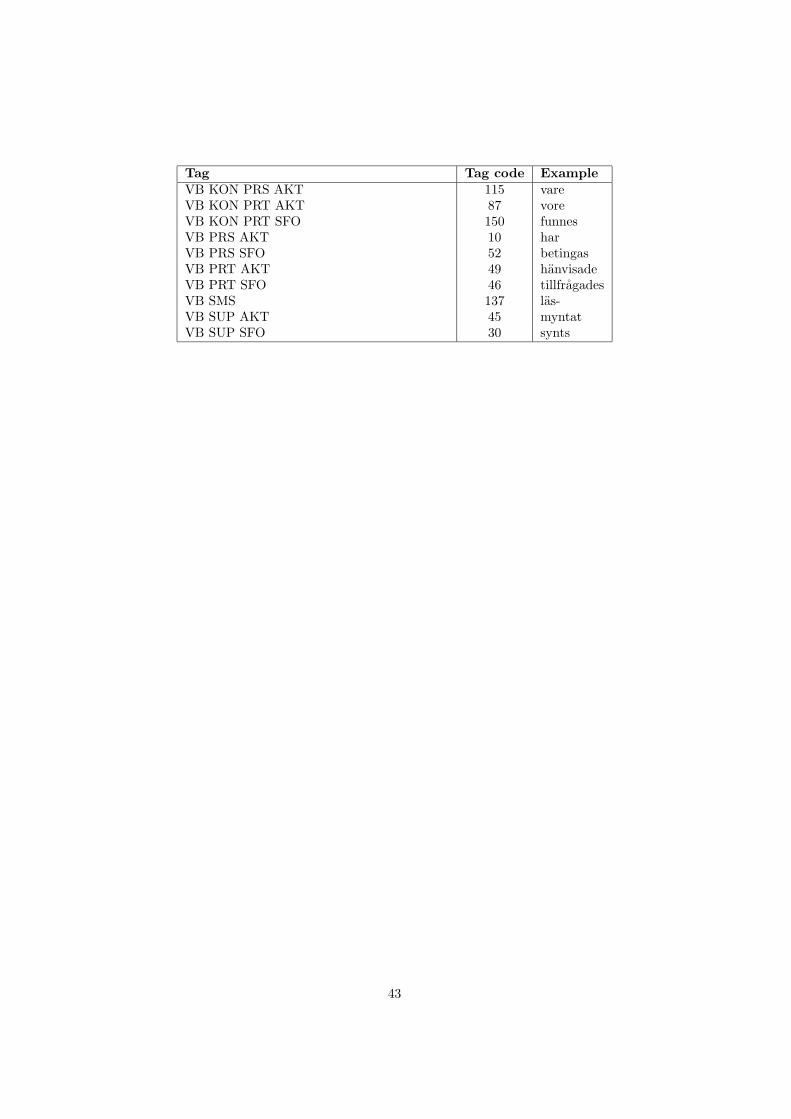
Tag Tag code ExampleVB KON PRS AKT 115 vareVB KON PRT AKT 87 voreVB KON PRT SFO 150 funnesVB PRS AKT 10 harVB PRS SFO 52 betingasVB PRT AKT 49 hanvisadeVB PRT SFO 46 tillfragadesVB SMS 137 las-VB SUP AKT 45 myntatVB SUP SFO 30 synts

43