A probabilistic analysis of randomly generated binary constraint satisfaction problems

Theoretical Computer Science 290 (2003) 1815–1828www.elsevier.com/locate/tcs

A probabilistic analysis of randomly generatedbinary constraint satisfaction problems

Martin Dyera ;1 , Alan Friezeb;∗;2 , Michael Molloyc;3aSchool of Computer Studies, University of Leeds, Leeds LS2 9JT, UK

bDepartment of Mathematical Sciences, Carnegie Mellon University, 5000 Forbes Avenue Pittsburgh,PA 15213, USA

cDepartment of Computer Science, University of Toronto, Toronto, Ont. M5S 3G4, Canada

Received 4 April 2001; received in revised form 18 February 2002; accepted 11 March 2002Communicated by M. Jerrum

1. Introduction

The constraint satisfaction problem (CSP) is a fundamental problem in Arti0cial In-telligence, with applications ranging from scene labelling to scheduling and knowledgerepresentation. See for example Dechter [4,7,10]. An instance of the CSP comprises aset of n variables, each taking a value in some given domain, and a set of constraintrelations, each of which determines the permitted joint values of a given subset of thevariables. The problem is either to determine any set of values for the variables whichrespects all the constraint relations, or prove that none exists.In recent years, there has been a strong interest in studying the relationship between

the input parameters that de0ne an instance of CSP (e.g. number of variables, domainsizes, tightness of constraints) and certain solution characteristics, such as the likeli-hood that the instance has a solution or the di9culty with which a solution may bediscovered. An extensive account of relevant results, both experimental and theoreti-cal, can be found in [2]. For a more recent discussion, see [9] which contains someexperimental work and theoretical discussion related to the results presented here.One of the most commonly used practices for conducting experiments with CSP is

to generate a large set of random instances, all with the same de0ning parameters, and

∗ Corresponding author.E-mail address: [email protected] (A. Frieze).1 Supported by EC Working Group RAND2.2 Supported by grants from NSF and EPSRC.3 Supported by NSERC and a Sloan Research Fellowship.

0304-3975/02/$ - see front matter c© 2002 Elsevier Science B.V. All rights reserved.PII: S0304 -3975(02)00317 -1

1816 M. Dyer et al. / Theoretical Computer Science 290 (2003) 1815–1828

then for each instance in the set to use heuristics for deciding if a solution exists. Notethat, in general CSP is NP-complete. The proportion of random instances that have asolution is used as an indication of the likelihood that an instance will be soluble, andthe average time taken per instance (by some standard algorithm) gives some measureof the hardness of such instances. A characteristic of many of these experiments is thatthe fraction of assignments of values that are permissible for each constraint is keptconstant as the number of variables increases.In this paper we consider only binary CSPs (BCSPs). These can be succinctly de-

scribed in the following way: A graph G=(V; E) is given, where V ={x1; x2; : : : ; xn}denotes the set of variables of the problem, and E the set of binary relations of theinstance. We assume, without loss of generality, that each variable can take values inthe same set [m]={1; 2; : : : ; m}. For each edge e={xi; xj}∈E, the relation can thenbe represented by an m×m 0–1 matrix Me, where 0 indicates that the pair of val-ues is forbidden and 1 that it is allowed. A solution to the associated BCSP is anassignment f :V → [m] of values to the variables, such that Me(f(xi); f(xj))=1 forall e={xi; xj}∈E. The aim of this paper is to conduct a probabilistic analysis of someaspects of the following simple random model of BCSP:Model: The underlying graph G is Gn;p1 for some 0¡p1=p1(n)¡1. (This means

that, with V ={x1; x2; : : : ; xn}, we let each of the ( n2 ) possible edges occur indepen-dently in E with probability p1.) For each edge e of G there is a random m×mconstraint matrix Me where Me(i; j)=0 or 1 independently with probability 1− p2 orp2, respectively, for some 0¡p2(n)¡1.We will discuss the e9cacy of various simple but standard approaches to solving

BCSPs. We analyse very simple algorithms in Theorems 1 and 2 and give tight thresh-old results for their e9cacy. We then consider tree search algorithms and prove somenegative results on their running times, Theorem 3. Finally, we consider the probabil-ity that a problem is unsatis0able because of some small substructure, Theorem 4. Adetailed description of our results follows.We 0rst consider the likely e9cacy of backtrack free search. Suppose the vertices

of G are ordered v1; v2; : : : ; vn. The width [5] w=w(v1; v2; : : : ; vn) of this order is givenby

w = maxi∈[n]

{|{ j: j ¡ i and vj is adjacent to vi}|}:

Thus, the width of the order is the maximum over i of the number of neighboursof vi which appear earlier in the order. For any graph G there is a minimum widthw∗(G) which is obtained as follows: Let v∗n be a vertex of minimum degree in G and,in general, let v∗i be a vertex of minimum degree in the subgraph of G induced byV\{v∗i+1; : : : ; v∗n}.The following simple backtrack free algorithm has been discussed in the literature:

Place the vertices of G into an optimal order v∗1 ; v∗2 ; : : : ; v

∗n giving a width w∗. Starting

with i=1 iteratively assign a value to vertex vi which is consistent with values alreadyassigned to v1; v2; : : : ; vi−1. We establish a sharp threshold for the likely success of thisalgorithm.

M. Dyer et al. / Theoretical Computer Science 290 (2003) 1815–1828 1817

Theorem 1. Suppose k¿3 is 6xed and

ck = min�¿0

��k e−�

k! + �k+1 e−�

(k+1)! + · · ·= min

�¿0

�Pr(Po(�)¿k − 1) ; (1)

where Po(�) denotes a Poisson random variable with mean �.Suppose ck¡c¡ck+1 and p1=c=n. Let �=(1−pk

2 )−1 and �¿0 be a positive con-

stant. Then• If m¿(1 + �) log� n then this algorithm succeeds whp. 1

• If m6(1− �) log� n then this algorithm fails whp.

Here failure means that at some step i, no value can be assigned to vertex vi whichis consistent with values already assigned to v1; v2; : : : ; vi−1. We are implicitly assum-ing that the assignment choices for v1; v2; : : : ; vi−1 are made without reference to theconstraints imposed by vi.The constants ck in (1) arise in the following way: The k-core of a graph G=(V; E)

is the (unique) largest set of vertices S that induces a subgraph G[S] with minimumdegree k. It is not di9cult to check that the optimal width w∗ for a graph G is themaximum k such that G has a k-core. The existence of k-cores in random graphs hasbeen well studied. The sharpest results are given in [8]. Let ck ; k¿3 be as de0nedin (1). It is proved there that if ck¡c¡ck+1 and p1=c=n then whp Gn;p1 has a k-core but no (k + 1)-core. In the context of width, this says that in the given rangew∗(Gn;p1 )=k whp.For example, c3≈3:35 and ck=k +

√k log k + O(log k) for large values of k, i.e.

the optimal width becomes asymptotic to the average degree. It is apparently believedthat, in practice, ordering by decreasing degree gives a reasonable approximation tothe width ordering, but we observe the following.

Remark 1. If one simply orders vertices in decreasing order of degree then whp oneobtains a width which asymptotically equal to

√log n= log log n, assuming that np1 is

bounded as n→∞.

Thus, asymptotically, this ordering will be arbitrarily bad compared with the mini-mum width ordering.Now consider the associated notion of strong k-consistency. A constraint satisfaction

problem is k-consistent if for all sets of vertices v; w1; w2; : : : ; wk and all consistentassignments a1; a2; : : : ; ak of values to w1; w2; : : : ; wk there is at least one assignmentvalue x for v which makes all the pairs v; wi have consistent assignments. The prob-lem is strongly k-consistent if it is i-consistent for 06i6k (note that k-consistencydoes not imply (k − 1)-consistency). We establish the following sharp threshold fork-consistency. It is identical to that of Theorem 1, except that the constraints on k; p1are now weaker but there is a lower bound constraint on p2.

1 With high probability, i.e. with probability tending to 1 as n → ∞.


Theorem 2. Let d=np1 and let �¿0 be a positive constant. Suppose

16 k = o(log n= log log n); (2)

|k log d| = o(log n); (3)

p2 ¿ n−�=(2k2): (4)

Let �=(1− pk2 )

−1. Then• If m¿(1 + �) log� n then the problem is strongly k-consistent, whp.• If m6(1− �) log� n then the problem is not k-consistent, whp.

Observe that we go from k-inconsistency whp to strong k-consistency as we passthe threshold level of m.We now consider the likely e9cacy of more sophisticated algorithms, which aim to

prove the inconsistency of BCSPs. We will consider values of the parameters whichensure that such algorithms fail whp.One basic strategy for solving a CSP is a tree search algorithm in which one moves

forward down the tree by selecting a vertex and making an assignment and whichbacktracks when it 0nds a set of vertices which, given the current assignments, haveno valid assignments left. Because of time constraints one can only check small setsof vertices for inconsistency, up to size K say. Our aim is to 0nd values for theparameters m; n; p1; p2; K such that any such algorithm is likely to take a long time to0nish, i.e. for any strategy for choosing which variable to set and which value to giveit. In Theorem 8 we give some rather complicated conditions. The following theoremgives some simpler but weaker conditions.First, observe that by computing the expected number of satisfying assignments we

see that if

np1(1− p2)¿ (2 + �) logm (5)

then the problem is unsatis0able whp.

Theorem 3. Assume (5) holds and that 16d=np1. Suppose that

K 6 max{3;

log n2 + log d

}; pD

2 ¿45; m=(log n)4 → ∞:

Then whp any tree search algorithm of the type described above must explore atleast mD nodes, for any D=o(m= log(m+ n)).

For example, if

m = d = (log n)5 and D = (log n)3 and p2 = 1− 15D

then the conditions of the theorem hold for any constant K and so whp any proof ofunsatis0ability by this method will take super-polynomial time.


The parameter D corresponds to the minimum depth to which we must whp explorebefore being able to backtrack because of inconsistency.If a problem is unsatis0able then one can hope to prove this by looking at small

sets of vertices and showing that they themselves form an unsatis0able subproblem.We give su9cient conditions for which this fails to happen whp.

Theorem 4. Assume that p2 is bounded below by a constant independent of n andthat a; b¿0 are arbitrary positive constants. Let �=(1− pk

2 )−1 and suppose that

C1. k=b log log n.C2. a¿2(1 + �)(1− p2)−1(1 + b logp−1

2 ).C3. p1=

a log log nn .

C4. m=(1 + �) log� n.

Then whp the problem is unsatis6able and every subproblem induced by a set of atmost !n; !=b=(3a) vertices is consistent.

2. Some probabilistic inequalities

In Theorems 5 and 6 below we will have a random variable Z=Z(Y1; Y2; : : : ; YN )where Yi∈%i are independent so that Z is de0ned on %=%1× · · ·%N .

Assumption 1. Suppose that Y; Y ′∈% and there exists i such that Yj=Y ′j for j = i. Our

assumption is that in such a case we have |Z(Y )− Z(Y ′)|6a.

Theorem 5 (Azuma–HoeKding inequality). If the random variable Z satis6es Assump-tion 1 then

Pr(|Z − E(Z)|¿ t)6 2 e−2t2=(Na2): (6)

Note that this is trivially applicable if Z=Y1+ · · ·+YN , where the Yi are independentand |Yi|6a for 16i6N .

Assumption 2. Suppose that, in addition, for any ', if Z(Y )¿' then there exist c(')indices j1; j2; : : : ; jc(') such that if Y ′

jt=Yjt for t=1; 2; : : : ; c(') then Z(Y ′)¿' also.Let MED=MED(Z) denote a median of Z i.e. Pr(Z¿MED)¿ 1

2 ; Pr(Z6MED)¿ 12 .

Theorem 6 (Talagrand’s inequality). If the random variable Z satis6es Assumptions 1and 2 then

Pr(|Z −MED|¿ tc(MED)1=2)6 2 e−t2=(4a2): (7)

The setting for the next inequality is diKerent. Let % be a set and A1; A2; : : : ; AN besubsets of %. Let X be a random subset of % where x∈% is independently placed into


X with probability p. Let Z denote the (random) number of sets Ai which X containsi.e. Z= |{i∈[N ]: X ⊇Ai}. We give an upper bound for the probability that Z=0. Let

*=∑

i �=j: Ai∩Aj �=∅Pr(Ai ∪ Aj ⊆ X )

=N∑i=1

Pr(Ai ⊆ X )∑

j: Ai∩Aj �=∅Pr(Aj\Ai ⊆ X ): (8)

Theorem 7 (Janson’s inequality).

Pr(Z = 0)6 exp{−E(Z)

2

*

}: (9)

Proofs of these inequalities can be found for example in [6].

3. Proof of Theorem 1

Consider an ordering v1; v2; : : : ; vn of the vertices which is formed by repeatedlychoosing a vertex of minimum degree in the subgraph induced by the vertices not yetlisted, and adding it to the end of the list. Let Vt={ j: vj has t neighbours amongv1; v2; : : : ; vj−1} for 16t6k be the set of indices j for which the vertex vj has exactlyt neighbours vi; i¡j. Since ck¡c¡ck+1 then whp V1; V2; : : : ; Vk partitions V , by thede0nition of ck .

Lemma 1. There exists +k¿0 (independent of n) such that whp |Vk |¿+kn.

Proof. Recall that we order the vertices by repeatedly choosing a vertex of minimumdegree in the subgraph induced by the vertices which are not yet listed, and we addthat vertex to the list. Since ck¡c¡ck+1, the graph a.s. has a k-core, H . Our procedurewill eventually reach H as the subgraph induced by the unlisted vertices, and then itwill, for the 0rst time, choose a vertex of degree k. We denote this time step by t.At any point during the ordering procedure, we denote by Wi the set of vertices of

degree i in the subgraph induced by the unlisted vertices. Consider the parameter

F =k(k − 1)|Wk |∑

i¿1 i|Wi| − 1:

De0ne � to be the largest solution to c=�=Pr(Po(�)¿k − 1) (note that � existsby the de0nition of ck). It is implicit from [8] that whp for each i¿k, the numberof vertices of degree i in H is !in+ o(n) where !i=Pr(Po(�)= i). (In particular, see(4.19) of [8] and the preceding discussion to see that at any point during their strippingprocedure, the proportion of remaining vertices which have degree i¿k is distributedas a Poisson with mean equal z (a parameter of the stripping process) truncated at


k; see (6.29) to see that in the terminal stages of the procedure, z=�; and see thestatement of their Theorem 2 to see that the total number of vertices in the k-core isnPr(Po(�)¿k). These three facts imply our claim.)From this, we will show that since c¿ck then whp at time t we have F¡−� for

some �=�(c)¿0.It is obvious that

k!k∑i¿k i!i

=1=(k − 1)!∑

i¿k �i−k =(i − 1)!

is strictly monotone decreasing as � increases. Therefore, it will su9ce to show thatif c were equal to ck then we would have k(k − 1)!k=

∑i¿k i!i=1.

First recall that at c=ck , � minimizes �=(1− e−� ∑k−2i=0 �i=i!). Setting the derivative

of this expression equal to 0 gives

1− e−�k−2∑i=0

�i

i!= �

(1− e−�

k−2∑i=0

�i

i!

)′

= �(e−�

k−2∑i=0

�i

i!− e−�

k−2∑i=1

�i−1

(i − 1)!)

= � e−�(

�k−2

(k − 2)!):

Multiplying both sides by e� yields

e� −k−2∑i=0

�i

i!=

∑i¿k−1

�i

i!=

�k−1

(k − 2)! :

Then multiplying both sides by � and shifting indices yields

∑i¿k

i�i

i!= k(k − 1) �

k

k!;

∑i¿k

i!i = k(k − 1)!k

as required.Furthermore, at each step of our procedure at most k + 1 vertices are either put in

the list or have their degrees reduced. Therefore, it is straightforward to verify thatthere is some 0=0(�)¿0 such that for the 0rst 0n steps of our procedure we will haveF¡−�=2.Expose the degree sequence of H . H is uniformly random with respect to its degree

sequence, see for example [8]. Thus, we can generate H according to the con0gurationmodel [1,3]. We will expose the pairs of the con0guration, i.e. the edges of H , asthey are exposed by our procedure. Therefore, when removing a vertex of degree i,its i neighbours are chosen at random from amongst all unlisted vertices, where theprobability that a vertex u is chosen is proportional to its degree.


For each j¿0 de0ne Xj to be the value of the sum |W1| + · · · + |Wk − 1| after thejth vertex has been removed, i.e. the number of remaining vertices of degree lessthan k. If Xj¿0 then upon adding the (j + 1)st vertex to our list, we select at mostk − 1 neighbours, reducing each of their degrees by one. The expected proportionof neighbours from Wk is k|Wk |=

∑i¿1 i|Wi|. If Xj=0 then Xj+16k. Therefore, it is

straightforward to verify that for j60n, Xj is statistically dominated by Yj de0ned as• Y0=0;• if Yj¿0 then Yj+1=Yj − 1 + BIN (k − 1; q), where (k − 1)q− 1= − �=2;• if Yj=0 then Yj+1=k.(In the second point, we use the fact that F¡−�=2.) The sequence Y0; Y1; : : : is arandom walk with negative drift and a reMective barrier at 0, and it is easy to con0rmthat a.s. the number of return-to-zeroes in this sequence before step 0n is at least 5nwhere 5=5(�; 0)¿0. Therefore, a.s. the number of return-to-zeroes of Xi is at least 5n.Each return-to-zero of Xi corresponds to another vertex being added to Vk . This provesthe lemma with +k=5.

Now consider vertex v. Let us say that v is “bad” if when the algorithm looks for anassignment for v it cannot 0nd anything consistent with assignments made previously.Instead of stopping at this point, let the algorithm make an arbitrary assignment. Henceif BAD is the set of bad vertices, the algorithm fails iK BAD =∅. If v∈Vt then

Pr(v ∈ BAD) = (1− pt2)

m

since we can generate the constraint matrix for v=va; vb; b¡a when we 0rst considerv. This matrix is not examined in any previous decisions. Now

E(|BAD||G) =k∑

t=0|Vt |(1− pt

2)m

6 n(1− pk2)

m

= n�−m

6 n−�

if m¿(1 + �) log� n.This veri0es the 0rst part of the theorem. Now assume that m6(1− �) log� n. Then

E(|BAD| | |Vk |¿+kn)¿ +kn�−m

¿ +kn�:

Given G we can write |BAD|=01 + 02 + · · · + 0n where the 0i are independent 0–1variables. This is because we do not need to generate Me for any e which contains viuntil we come to make the assignment to vi. Thus, the probability that 0i=1 does notdepend on the values of 01; 02; : : : ; 0i−1. Then we can use (6) to show concentrationround the mean. In particular |BAD|¿0 whp.



Let Zt count the number of choices of vertices v and neighbours w1; w2; : : : ; wt of vfor which there exist consistent assignments a1; a2; : : : ; at such that there is no consistentchoice of a value for v. The problem is strongly k-consistent iK Z=Z0+Z1+· · ·+Zk=0.Now

E(Z)6k∑

t=0n(n− 1t

)pt1 Pr(∃choices a1; a2; : : : ; at)

6k∑

t=0n(n− 1t

)pt1m

t(1− pt2)

m

6 nk∑

t=1(md)t(1− pt

2)m

6 kn(m(d+ 1))k�−m:

If m¿(1 + �) log� n then

E(Z)6 kn−�((d+ 1)(1 + �) log� n)k 6 kn−�=2((d+ 1)(1 + �) log n)k = o(1)

after using (2)–(4). So in this case Z=0 whp proving the 0rst part of the theorem.Suppose next that m6(1−�) log� n. Let Zk denote the number of choices of vertices

v, neighbours w1; w2; : : : ; wk of v such that w1; w2; : : : ; wk form an independent set andassignments a1; a2; : : : ; ak for w1; w2; : : : ; wk such that there is no consistent choice of avalue for v. Then

E(Zk)¿ n(n− 1k

)pk1(1− O(k2p1))�−m;

where the (1−O(k2p1)) term is the probability that the chosen vertices w1; w2; : : : ; wk

form an independent set and we only consider one assignment to w1; w2; : : : ; wk . So,after using Stirling’s inequality,

E(Zk)¿n

2√k

(edk

)k

�−m

¿n�

2√k

(edk

)k

¿ n�−o(1):

We will apply Talagrand’s inequality to a slight modi0cation of this variable. Thus,let Zk be Zk where in the count for each v we only include w1; w2; : : : ; wk from the�=(d + 1)(log n)2 lowest indexed neighbours of v. Now, with *(G) denoting the


maximum degree of G, we have

Pr(*(G)¿ �)6 n(n�

)p�1 6 n(nep1=�)� 6 (log n)−(2−o(1))(log n)

2

= o(n−(k+1)):

Thus

Zk = Zk whp:

Furthermore, Zk6nk+1 and so we see that

E(Zk) = E(Zk) + o(1)¿ n�−o(1):

Now consider the probability space for our problem to be %N ; N=( n2 ) where % is theset of m×m 0–1 matrices i.e. one matrix Me for each edge e of Kn. Then if 6=6(M)denotes the number of 1’s in matrix M we let

Pr(Me = M) =

{p1p6

2(1− p2)m2−6; 6 = m2;

(1− p1) + p1pm22 ; 6 = m2;

(6=m2 implies M is a matrix of all 1’s and when e is not an edge of Gn;p1 we let Me

be the matrix of all 1’s. Of course, Me is only relevant if e is in our constraint graph,but for technical reasons it is convenient here to generate Me for every e∈Kn.)Now changing one matrix Me can change Zk by at most 2�k=no(1). Furthermore, if

Zk¿' then we can 0nd at most (k+1)' indices (edges) which force Zk¿'. ApplyingTalagrand’s inequality we get

Pr(|Zk −MED(Zk)|¿ t((k + 1)MED(Zk))1=2)6 exp{−t2=(4�2k)}:

Putting t=n�=3 we see that E(Zk)=MED(Zk) + O(n�=3+o(1)(MED(Zk))1=2). So we seethat MED(Zk)¿n�−o(1) and then that Zk= Zk =0 whp.


We prove the following theorem which has a more complex set of conditions onthe various parameters. It is simple to verify that the conditions of Theorem 3 implythese.

Theorem 8. Assume (5) holds and that 16d=np1. Suppose that

K 6 max{3;

log n2 + log d

}; (10)


p−11 K(de22m)K exp

{− m2p22K(K + 1)2

}→ 0 as n → ∞; (11)

p−11 2m(dm)D(1− pD

2 )m=2 → 0: (12)

Then whp any tree search algorithm of the type described above must explore atleast mD nodes.

First of all we verify that the expected number of solutions is o(1). Let A denotethe number of consistent assignments.

E(A) = mn(1− p1(1− p2))(n2

)6 exp

{−n

(n− 12

p1(1− p2)− logm)}

and this tends to zero if (5) holds.Consider the following conditions:

C1. There exists a set of vertices S={v1; v2; : : : ; vk}; k6K which induce a connectedsubgraph of G and sets B1; B2; : : : ; Bk ⊆ [m], each of size m0=�m=2� such thatthere are no feasible assignments ai; i=1; 2; : : : ; k for v1; v2; : : : ; vk for whichai∈Bi; i=1; 2; : : : ; k.

C2. There exists a vertex v, neighbours u1; : : : ; u‘∈V of v where ‘6D, and assign-ments to u1; : : : ; u‘ such that v has fewer than m0 choices of assignment whichare consistent with those of u1; : : : ; u‘.

If neither C1 nor C2 occur and the problem is unsatis0able then the algorithm mustexplore at least mD nodes. At depth 6D every vertex which has not been assigneda value will still have at least m0 choices of assignment which are consistent withany given to its neighbours ( RC2). Then each set of K vertices will have a mutuallyconsistent set of choices ( RC1).We observe 0rst that (10) implies that whp every set of k6K vertices of G contains

at most k + 1 edges. Then (10) implies d6n1=K e−6. The probability that there existsa set of k6K vertices of G containing at least k + 2 edges is at most

K∑k=4

(nk

)( (k2

)k + 2

)pk+21 6

K∑k=4

(nek

)k(ke2

)k+2(dn

)k+2

6(eKd2n

)2 K∑k=4

(e2d2

)k

6(

Kn1−1=K

)2 K∑k=4

(n1=K

2 e4

)k

¡ n(

Kn1−1=K

)2= o(1)

when K¿4 (for K¡4 the sum is empty).


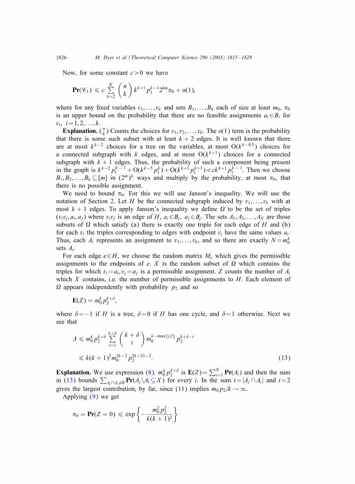
Now, for some constant c¿0 we have

Pr(C1)6 cK∑

k=2

(nk

)kk+1pk−1

1 2km90 + o(1);

where for any 0xed variables v1; : : : ; vk and sets B1; : : : ; Bk each of size at least m0, 90is an upper bound on the probability that there are no feasible assignments ai∈Bi forvi; i=1; 2; : : : ; k.Explanation. ( nk ) Counts the choices for v1; v2; : : : ; vk . The o(1) term is the probability

that there is some such subset with at least k + 2 edges. It is well known that thereare at most k k−2 choices for a tree on the variables, at most O(k k−0:5) choices fora connected subgraph with k edges, and at most O(k k+1) choices for a connectedsubgraph with k + 1 edges. Thus, the probability of such a component being presentin the graph is k k−2pk − 1

1 +O(k k−5pk1 )+O(k

k+1pk+11 )¡ckk+1pk − 1

1 . Then we chooseB1; B2; : : : ; Bk ⊆ [m] in (2m)k ways and multiply by the probability, at most 90, thatthere is no possible assignment.We need to bound 90. For this we will use Janson’s inequality. We will use the

notation of Section 2. Let H be the connected subgraph induced by v1; : : : ; vk with atmost k + 1 edges. To apply Janson’s inequality we de0ne % to be the set of triples(vivj; ai; aj) where vivj is an edge of H , ai∈Bi; aj∈Bj. The sets A1; A2; : : : ; AN are thosesubsets of % which satisfy (a) there is exactly one triple for each edge of H and (b)for each vi the triples corresponding to edges with endpoint vi have the same values ai.Thus, each Ai represents an assignment to v1; : : : ; vk , and so there are exactly N=mk

0sets Ai.For each edge e∈H , we choose the random matrix Me which gives the permissible

assignments to the endpoints of e. X is the random subset of % which contains thetriples for which vi=ai; vj=aj is a permissible assignment. Z counts the number of Aiwhich X contains, i.e. the number of permissible assignments to H . Each element of% appears independently with probability p2 and so

E(Z) = mk0p

k+02 ;

where 0=−1 if H is a tree, 0=0 if H has one cycle, and 0=1 otherwise. Next wesee that

*6mk0p

k+02

k+0∑t=1

(k + 0t

)mk−max{t;2}0 pk+0−t

2

6 k(k + 1)2m2k−20 p2k+20−22 : (13)

Explanation. We use expression (8). mk0p

k+02 is E(Z)=

∑Ni=1 Pr(Ai) and then the sum

in (13) bounds∑

Aj∩Ai �=∅ Pr(Aj\Ai ⊆X ) for every i. In the sum t= |Aj ∩Ai| and t=2gives the largest contribution, by far, since (11) implies m0p2=k→∞.Applying (9) we get

90 = Pr(Z = 0)6 exp{− m20p

22

k(k + 1)2

}


and so

Pr(C1)6 cK∑

k=1p−11 k(de2m)k exp

{− m20p

22

k(k + 1)2

}→ 0

which follows directly from (11).Now consider C2.

Pr(C2)6 nD∑

‘=1

(n‘

)p‘1m

‘(

mm− m0 + 1

)(1− p‘

2)m−m0+1

6 nD∑

‘=1(dm)‘2m(1− pD

2 )m=2

→ 0:


First note that m6(1 + �)p−k2 log n and so

np1(1− p2)

¿ 2(1 + �)(1 + b logp−12 ) log log n = 2(1 + �)(log log n+ k logp−1

2 )

¿ (2 + �) logm

and so by (5) the problem is unsatis0able whp.We deduce from C1 and C4 and Theorem 2 that whp the problem is strongly k-

consistent. We prove next that whp every set S of s6!n vertices induces a subgraphwith fewer than ks=2 edges. Thus, if |S|6!n and H=G[S] is the subgraph of G inducedby S, then H has no k-core and so the algorithm of Theorem 1 will 0nd an assignmentwhich is consistent for the sub-problem induced by H .Now

Pr(∃S; |S|6 !n containing¿ k|S|2 edges)6

!n∑s=k+1

(ns

)( (s2

)ks=2

)pks=21

6!n∑

s=k+1

(nes

( seabn

)k=2)s

= o(1):

Remark 2. We see from the proof that if a¡ 13b then whp there is no k-core and the

problem itself is k-consistent. So presumably there is a transition from being solvableby a simple backtrack free algorithm to infeasible as a increases. Whether this transitionis sharp is unclear.


References

[1] E.A. Bender, E.R. Can0eld, The asymptotic number of labelled graphs with given degree sequence,J. Combin. Theory A 24 (1978) 296–307.

[2] D.G. Bobrow, M. Brady (Eds.), in: T. Hogg, B.A. Hubermann, C.P. Williams (Guest Eds.), SpecialVolume on Frontiers in Problem Solving: Phase Transitions and Complexity, North-Holland, Amsterdam,New York, Arti0cial Intelligence 81(1,2) (1996).

[3] B. BollobTas, A probabilistic proof of an asymptotic formula for the number of labelled regular graphs,Euro. J. Combin. 1 (1980) 311–316.

[4] R. Dechter, Constraint networks, in: S. Shapiro (Ed.), Encyclopedia of Arti0cial Intelligence, 2ndEdition, Wiley, New York, 1992, pp. 276–285.

[5] E.C. Freuder, A su9cient condition for backtrack-free search, J. ACM 29 (1982) 24–32.[6] S. Janson, T. Luczak, A. RuciTnski, Random Graphs, Wiley, New York, 2000.[7] A.K. Mackworth, Constraint satisfaction, in: S. Shapiro (Ed.), Encyclopedia of Arti0cial Intelligence,

2nd Edition, Wiley, New York, 1992, pp. 285–293.[8] B. Pittel, J. Spencer, N. Wormald, Sudden emergence of a giant k-core in a random graph, J. Combin.

Theory B 67 (1996) 111–151.[9] B.M. Smith, Constructing an asymptotic phase transition in random binary constraint satisfaction

problems, Research Report 2000.02, University of Leeds, January 2000. (To appear in TheoreticalComputer Science: Special Issue on NP-Hardness and Phase Transitions.)

[10] D. Waltz, Understanding line drawings of scenes with shadows, in: P.H. Winston (Ed.), The Psychologyof Computer Vision, McGraw-Hill, New York, 1975, pp. 19–91.

Documents

A probabilistic analysis of randomly generated binary constraint satisfaction problems