University of Kentucky University of Kentucky

UKnowledge UKnowledge

Theses and Dissertations--Epidemiology and Biostatistics College of Public Health

2017

A PREDICTIVE PROBABILITY INTERIM DESIGN FOR PHASE II A PREDICTIVE PROBABILITY INTERIM DESIGN FOR PHASE II

CLINICAL TRIALS WITH CONTINUOUS ENDPOINTS CLINICAL TRIALS WITH CONTINUOUS ENDPOINTS

Meng Liu University of Kentucky, meng.liu@uky.edu Digital Object Identifier: https://doi.org/10.13023/ETD.2017.334

Right click to open a feedback form in a new tab to let us know how this document benefits you. Right click to open a feedback form in a new tab to let us know how this document benefits you.

Recommended Citation Recommended Citation Liu, Meng, "A PREDICTIVE PROBABILITY INTERIM DESIGN FOR PHASE II CLINICAL TRIALS WITH CONTINUOUS ENDPOINTS" (2017). Theses and Dissertations--Epidemiology and Biostatistics. 15. https://uknowledge.uky.edu/epb_etds/15

This Doctoral Dissertation is brought to you for free and open access by the College of Public Health at UKnowledge. It has been accepted for inclusion in Theses and Dissertations--Epidemiology and Biostatistics by an authorized administrator of UKnowledge. For more information, please contact UKnowledge@lsv.uky.edu.

STUDENT AGREEMENT: STUDENT AGREEMENT:

I represent that my thesis or dissertation and abstract are my original work. Proper attribution

has been given to all outside sources. I understand that I am solely responsible for obtaining

any needed copyright permissions. I have obtained needed written permission statement(s)

from the owner(s) of each third-party copyrighted matter to be included in my work, allowing

electronic distribution (if such use is not permitted by the fair use doctrine) which will be

submitted to UKnowledge as Additional File.

I hereby grant to The University of Kentucky and its agents the irrevocable, non-exclusive, and

royalty-free license to archive and make accessible my work in whole or in part in all forms of

media, now or hereafter known. I agree that the document mentioned above may be made

available immediately for worldwide access unless an embargo applies.

I retain all other ownership rights to the copyright of my work. I also retain the right to use in

future works (such as articles or books) all or part of my work. I understand that I am free to

register the copyright to my work.

REVIEW, APPROVAL AND ACCEPTANCE REVIEW, APPROVAL AND ACCEPTANCE

The document mentioned above has been reviewed and accepted by the student’s advisor, on

behalf of the advisory committee, and by the Director of Graduate Studies (DGS), on behalf of

the program; we verify that this is the final, approved version of the student’s thesis including all

changes required by the advisory committee. The undersigned agree to abide by the statements

above.

Meng Liu, Student

Dr. Emily Van Meter Dressler, Major Professor

Dr. Steve Browning, Director of Graduate Studies

A PREDICTIVE PROBABILITY INTERIM DESIGN FOR PHASE II CLINICAL

TRIALS WITH CONTINUOUS ENDPOINTS

DISSERTATION

A dissertation submitted in partial fulfillment of the

requirements for the degree of Doctor of Philosophy in the

College of Public Health

at the University of Kentucky

By

Meng Liu

Lexington, Kentucky

Co-Directors: Dr. Emily V. Dressler , Professor of Biostatistics

and Dr. Heather Bush , Professor of Biostatistics

Lexington, Kentucky

Copyright © Meng Liu 2017

ABSTRACT OF DISSERTATION

A PREDICTIVE PROBABILITY INTERIM DESIGN FOR PHASE II CLINICAL

TRIALS WITH CONTINUOUS ENDPOINTS

Phase II clinical trials aim to potentially screen out ineffective and identify effective

therapies to move forward to randomized phase III trials. Single-arm studies remain the

most utilized design in phase II oncology trials, especially in scenarios where a randomized

design is simply not practical. Due to concerns regarding excessive toxicity or ineffective

new treatment strategies, interim analyses are typically incorporated in the trial, and the

choice of statistical methods mainly depends on the type of primary endpoints. For

oncology trials, the most common primary objectives in phase II trials include tumor

response rate (binary endpoint) and progression disease-free survival (time-to-event

endpoint). Interim strategies are well-developed for both endpoints in single-arm phase II

trials.

The advent of molecular targeted therapies, often with lower toxicity profiles from

traditional cytotoxic treatments, has shifted the drug development paradigm into

establishing evidence of biological activity, target modulation and pharmacodynamics

effects of these therapies in early phase trials. As such, these trials need to address

simultaneous evaluation of safety as well as proof-of-concept of biological marker activity

or changes in continuous tumor size instead of binary response rates.

In this dissertation, we extend a predictive probability design for binary outcomes

in the single-arm clinical trial setting and develop two interim designs for continuous

endpoints, such as continuous tumor shrinkage or change in a biomarker over time. The

two-stage design mainly focuses on the futility stopping strategies, while it also has the

capacity of early stopping for efficacy. Both optimal and minimax designs are presented

for this two-stage design. The multi-stage design has the flexibility of stopping the trial

early either due to futility or efficacy. Due to the intense computation and searching

strategy we adopt, only the minimax design is presented for this multi-stage design. The

multi-stage design allows for up to 40 interim looks with continuous monitoring possible

for large and moderate effect sizes, requiring an overall sample size less than 40. The

stopping boundaries for both designs are based on predictive probability with normal

likelihood and its conjugated prior distributions, while the design itself satisfies the pre-

specified type I and type II error rate constraints. From simulation results, when compared

with binary endpoints, both designs well preserve statistical properties across different

effect sizes with reduced sample size. We also develop an R package, PPSC, and detail it

in chapter four, so that both designs can be freely accessible for use in future phase II

clinical trials with the collaborative efforts of biostatisticians. Clinical investigators and

biostatisticians have the flexibility to specify the parameters from the hypothesis testing

framework, searching ranges of the boundaries for predictive probabilities, the number of

interim looks involved and if the continuous monitoring is preferred and so on.

KEYWORDS: Predictive Probability, Continuous Endpoints, Single-Arm, Phase II Trials,

Interim Strategy, R package

______________________Meng Liu_____

____________ _______July 17, 2017____

Date

A PREDICTIVE PROBABILITY INTERIM DESIGN FOR PHASE II CLINICAL

TRIALS WITH CONTINUOUS ENDPOINTS

By

Meng Liu

__ ____Emily Van Meter Dressler_______

Co-Director of Dissertation

________________ Heather Bush ___________

Co-Director of Dissertation

_______________Steve Browning___ ________

Director of Graduate Studies

_______________________July 17, 2017_____

Date

To my parents Hua Li and Hongwei Liu

iii

ACKNOWLEDGEMENT

I would like to thank my committee for continued guidance over the past five years.

The most important acknowledgement of gratitude I wish to express is to my mentor and

supervisor, Dr. Emily Dressler, who is always here when I need help or get into panic. I

am grateful for her excellent guidance, caring, patience and providing me with her expertise

to tackle each problem in this dissertation work. It was only due to her valuable guidance

and cheerful enthusiasm that I was able to complete my dissertation work. I would also like

to thank Dr. Heather Bush, who keeps giving me guidance and inspirations since I entered

this program, and providing me with all the potential research areas when I had no idea

about the future. I would like to thank Dr. Heidi Weiss and Dr. Erin Abner for being in my

committee and providing valuable advice for my dissertation to keep me on track. I would

like to thank Dr. Aju Mathew for being willing to serve in my committee and providing

clinical insights of this work. I would also like to thank Dr. Markos Leggas for being my

outside examiner and providing support during the defense process.

I would like to thank everyone in the BBSRF, from whom I have learnt so much

about clinical trials as a GRA for the past four years and decided to pursue a career in this

field. I would like to thank Dr. Brent Shelton for bringing me to this wonderful and friendly

group. I would like to thank Stacey Slone and Jinpeng Liu for helping me out whenever I

am stuck in any coding problems. Also, I would like to thank all my cohort classmates,

without whom I would never have the courage and confidence to pass through all the

courses and exams. It has been a grateful and amazing journey during the past five years.

Finally, I would like to thank my parents for your love, encouragement and

constantly support during the past eight years. Thank you both for believing in me, wanting

the best for me and inspiring me to follow my dreams. Your love and support is the greatest

gift in my life.

iv

TABLE OF CONTENTS

Acknowledgments ............................................................................................................. iii

Table of Contents ................................................................................................................v

List of Tables .................................................................................................................... vi

List of Figures .................................................................................................................. vii

Chapter One: Introduction ..................................................................................................1

1.1 Current Endpoints in Oncology Phase II Clinical Trials .........................................1

1.2 Importance of Single-Arm Trials .............................................................................2

1.3 Current Phase II Trial Designs .................................................................................3

1.3.1 Importance of Interim Strategies in the Trial ......................................................3

1.3.2 Frequentist Designs for Binary Outcome ............................................................3

1.3.3 Bayesian Designs for Binary Outcome ...............................................................6

1.3.4 Bayesian vs. Frequentist Approaches ..................................................................9

1.3.5 Designs for Continuous Endpoints ....................................................................11

Chapter Two: A Two-Stage Predictive Probability Interim Design for Phase II

Clinical Trials with Continuous Endpoints

2.1 Abstract ..................................................................................................................15

2.2 Introduction ............................................................................................................16

2.3 Methods ..................................................................................................................18

2.3.1 Notation and Proposed Design ..........................................................................18

2.3.2 Trial Decision Rules ..........................................................................................21

2.3.3 Frequentist Operating Characteristics ...............................................................23

2.3.4 Optimization Criteria .........................................................................................24

2.4 Results ....................................................................................................................25

2.4.1 Roles of Priors ...................................................................................................28

2.4.2 Case Study .........................................................................................................29

2.5 Discussion ..............................................................................................................30

Chapter Three: A Multi-Stage Predictive Probability Interim Design for Phase

II Clinical Trials with Continuous Endpoints

3.1 Abstract ..................................................................................................................41

3.2 Introduction ............................................................................................................41

3.3 Methods ..................................................................................................................43

3.3.1 Notation and Proposed Design ..........................................................................43

3.3.2 Trial Decision Rules ..........................................................................................46

v

3.3.3 Frequentist Operating Characteristics ...............................................................46

3.3.4 Optimization Criteria .........................................................................................48

3.4 Results ....................................................................................................................49

3.4.1 Roles of Priors ...................................................................................................50

3.4.2 Case Study .........................................................................................................51

3.5 Discussion ..............................................................................................................52

Chapter Four: PPSC: An R Package for Single-Arm Phase II Predictive

Probability Design with Continuous Endpoints

4.1 Abstract ..................................................................................................................63

4.2 Introduction ............................................................................................................63

4.3 Methods ..................................................................................................................65

4.4 Use of Package PPSC .............................................................................................68

4.4.1 Two-Stage Design for Early Stopping due to Futility: Use of par2stage ........70

4.4.2 Multi-Stage Design for Early Stopping due to Both Futility and Superiority:

Use of parmultistage ..................................................................................................77

4.5 Discussion .............................................................................................................82

Chapter Five: Conclusion .................................................................................................86

5.1 Conclusion ..............................................................................................................86

5.2 Strengths and Limitations .......................................................................................88

5.3 Future Directions ....................................................................................................90

Appendices.........................................................................................................................93 Bibliography ....................................................................................................................112

Vita ...................................................................................................................................117

vi

LIST OF TABLES

Table 2.1 Operating characteristics of optimal design for continuous endpoints with early

termination for futility……………………………………………………………35

Table 2.2 Operating characteristics of minimax design for continuous endpoints with early

termination for futility……………………………………………………………36

Table 2.3 Operating characteristics of optimal design for continuous endpoints with early

termination for efficacy……………………..………...……….………….……...37

Table 2.4 Operating characteristics of minimax design for continuous endpoints with early

termination for efficacy……………………..……………….……………….…..38

Table 2.5 Operating characteristics of optimal designs with different priors………….….39

Table 2.6 Operating characteristics of minimax designs with different priors…………....39

Table 2.7 Operating characteristics of optimal design and minimax design for case

study……………………………………………………………………………...40

Table 3.1 Operating characteristics of minimax multi-stage design for continuous

endpoints………………………………………………………...........………….56

Table 3.2 Operating characteristics of minimax designs with different priors……………58

Table 3.3 Operating characteristics of 5-stage and 10-stage minimax design with equal

space for case study………………………………………………………………61

Table 3.4 Operating characteristics of 5-stage unequal space for case study…………….61

Table 4.1 Input options for function par2stage……………………………………..……84

Table 4.2 Input options for function parmultistage………………………………………85

vii

LIST OF FIGURES

Figure 1.1 Flowchart of Simon’s two-stage design………………………………….……14

Figure 2.1 Proposed two-stage PP design for continuous endpoints………………….…..34

Figure 3.1: Stopping boundaries for the 10-stage design with 4 different priors …………60

Figure 3.2: Stopping boundaries for the 5-stage design and 10-stage design for case

study……………………………………………….....…………………………..62

1

CHAPTER ONE

Introduction

1.1 Current Endpoints in Oncology Phase II Clinical Trials

In oncology clinical trials, overall survival (OS) has been the gold standard, and

considered to be the most clinically relevant and reliable primary endpoint for definitive

phase III randomized clinical trials. Therefore, a good endpoint that can predict the overall

survival effectively in phase II trials is vital in drug development. In practice, tumor

shrinkage is divided into the response rate (RR) according to the Response Evaluation

Criteria in Solid Tumors (RECIST) criteria, with a cut-off value of 30%. Both response

rate and progression-free survival (PFS) are commonly used as surrogate endpoints for

efficacy in current phase II trials [1, 2].

One of the major challenges in drug development is the efficient design of phase II

trials to identify active compounds for phase III testing. The failure to accurately predict

effective drugs/treatments in early phase trials causes a disproportionately high incidence

of phase III trials with negative results. It has been reported that only 5% of treatments

tested in the phase III setting are approved in oncology [2]. Therefore, there is a need to

screen agents in the phase II setting quickly and effectively, while using more robust

endpoints predictive of overall survival (OS) and clinical benefit that will predict phase III

success, and balance resources to prioritize those therapies deemed promising, especially

for novel therapeutics or targeted agents. Endpoints to consider include: continuous tumor

size, quality of life outcomes, molecular biomarkers, and imaging assessment [3, 4].

Since trial design, sample size consideration, analysis plans and interim properties

completely depend on the type of outcome variable selected, choice of endpoints is of great

2

importance before the trial starts. In terms of oncology trials, although response rate has

been widely used in practice, studies have shown that designs using binary response rate

require many more patients than those using continuous tumor size shrinkage, and lead to

loss of statistical efficiency [5, 6]. In addition, drugs can be still active even if they do not

lead to a high-level of tumor regression; thus, in this case, a change in a biomarker over

time might be more helpful. Further, previous studies have shown that for specific types of

cancer, such as patients with metastatic renal cell carcinoma and treated with target

therapies, early primary tumor size reduction, which is about 10% tumor shrinkage, is an

independent predictor of improved overall survival. In these situations, RECIST criteria

may not be appropriate [1]. Therefore, using continuous tumor size as the primary endpoint

has been investigated and shown to be potentially clinically beneficial [7, 8].

1.2 Importance of Single-Arm Trials

Although randomized phase II trials, including but not limited to selection designs,

screening designs, and randomized discontinuation designs, are gaining popularity with

clinical researchers, single-arm studies still remain the most utilized design in phase II

oncology trials, especially in scenarios where a randomized design is simply not practical

[9-11]. Those scenarios include a low likelihood of response to standard therapies, the

mechanism of action expected to be cytotoxic, the desired effect size being large, and

historical controls remaining stable over time. In particular, with the development of

molecular target therapies in oncology recent years, single-arm trials still remain the most

feasible design to conduct in practice, especially for smaller centers or investigator initiated

trials when the science is novel, and it would be otherwise impossible with available

3

resources to obtain preliminary data to then justify a larger, multi-center trial. These

situations are quite common for rare tumors or subtypes and gynecologic cancers [12, 13].

1.3 Current Phase II Trial Designs

1.3.1 Importance of Interim Strategies in the Trial

Interim strategies are of great importance in each stage of oncology clinical trials.

Developed to protect participants from unsafe drugs or to hasten the general

implementation of a beneficial therapy, interim strategies can be utilized to stop trials early

either for safety, futility, or efficacy [14]. In addition, interim monitoring in the trial

can help identify the need to collect additional data in order to clarify questions of

clinical benefit or safety issues that may arise during the trial. It can further help reveal

logical problems or issues involving data quality that need to be promptly addressed. Thus,

incorporating appropriate interim strategies in the trials will facilitate the success of the

trial and benefit patients, as well as save time and resources [15-17]. In particular, for phase II

trials, which usually have a smaller sample size and relatively short in duration, enough

information must be obtained to decide whether the trials should be stopped for lack of

evidence suggesting safety or efficacy, or whether the trials should be continued and moved

forward to confirmatory phase III testing for evidence demonstrating efficacy. An

appropriate stopping rule can lead quickly to an indication and facilitate the decision

making.

1.3.2 Frequentist Designs for Binary Outcome

During past decades, many statistical methods have been proposed and developed

for phase II trial designs. Gehan proposed a two-stage design, in which early termination

4

depends on the number of responses in the first stage. If there is no response at the end of

the first stage, the trial is stopped for futility; otherwise, continue to the second stage [18].

Simon developed both optimal and minimax design for a single-arm two-stage setting [19],

which has been the most widely used single-arm design for phase II studies with binary

outcomes. Simon’s two-stage design has been extended and developed into different

directions in the literature and practice. In particular, Chen extended Simon’s design into a

three-stage design that allows early termination of the trial due to futility and 10% average

sample size reduction when compared to the two-stage design [20]. Bryant and Day

incorporated toxicity into the design to monitor both efficacy and toxicity simultaneously

[21], which was then extended into both two-stage and multi-stage designs for dependent

variables and control of the type I/II error rates at the same time [22, 23]. Lin et al. extended

Simon’s design into a two-stage setting that can utilize both primary and secondary

endpoints, both of which are assumed to be binary outcomes [24]. Jung et al. developed a

graphical method to search for a compromise between optimal and minimax designs [25].

Since two-stage designs are still the most widely used in practice for early phase II trials,

especially with the popularity of Simon’s two-stage design, we detail the Simon’s two-

stage design below.

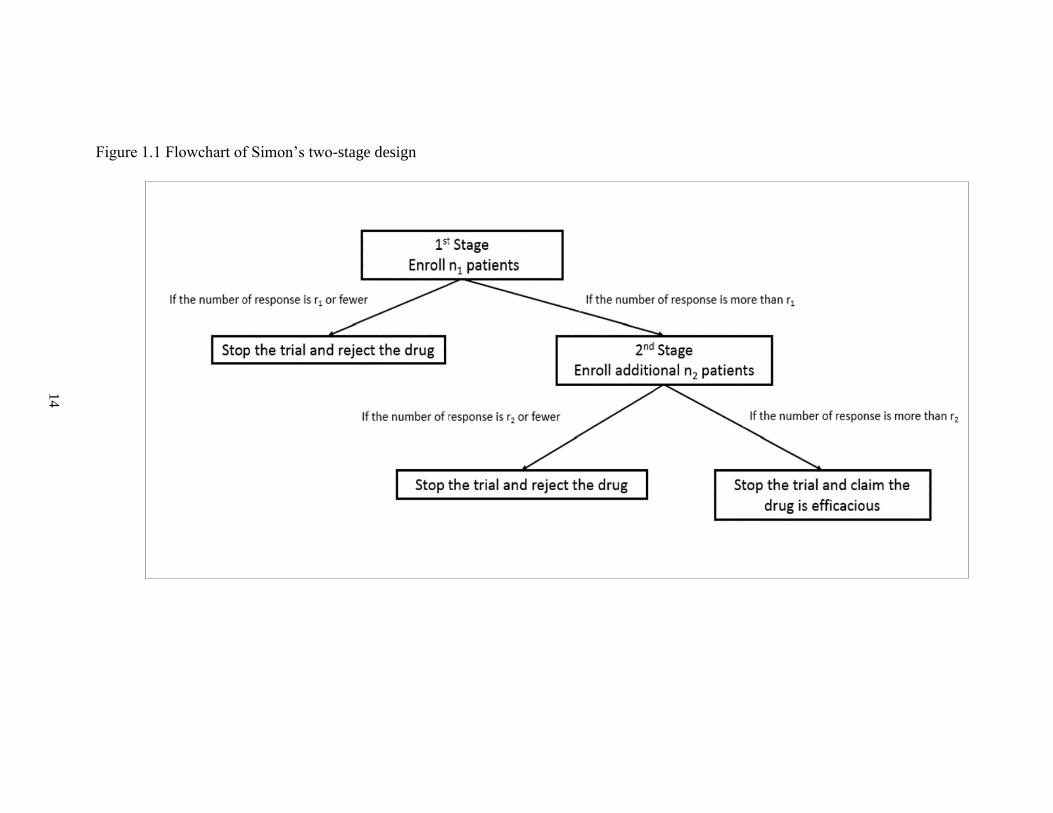
Simon’s two-stage design

Simon's two-stage design for terminating the trial early due to futility has been the

most commonly applied design in single-arm cancer clinical trials [19]. The design can be

illustrated in Figure 1.1. In his design, the primary endpoint is the binary response rate.

During the first stage, 𝑛1 patients are enrolled. If the number of patients with responses

within these 𝑛1 patients is less than or equal to 𝑟1, the trial should be terminated early for

5

futility. Otherwise, we should move forward to the second stage and enroll additional

𝑛2 patients. If the number of responses at the second stage is less than 𝑟2, we should stop

the trial and claim that this new therapy is not effective and not worth further investigating.

𝑟1 and 𝑟2 are the critical values for the number of responses at the end of each stage .

Mathematically, let the true probability of response be 𝑝, which follows a binomial

distribution. Let 𝑝 ≤ 𝑝0 represents the drug/therapy with low activity that should be

screened out from further testing, and 𝑝 ≥ 𝑝1 represents a drug/therapy with sufficient

activity to warrant further phase III testing. 𝑝0 is some uninteresting level of response rate

and 𝑝1 is a desirable target level. A typical hypothesis testing can be stated:

𝐻0: 𝑝 ≤ 𝑝0 vs. 𝐻1: 𝑝 ≥ 𝑝1

Let X denote the number of responses at the 1st stage.

1. If the drug is rejected at the end of the 1st stage, the total number of responses at

the end of the 1st stage is less than 𝑟1. Thus, the probability of rejecting a drug (failing to

reject the null hypothesis) with response probability 𝑝 is:

Pr(𝑋 ≤ 𝑟1) = ∑𝑏(𝑥; 𝑝, 𝑛1)

𝑟1

𝑥=0

= 𝐵(𝑟1; 𝑝, 𝑛1)

where 𝑏(𝑥; 𝑝, 𝑛1) is the probability mass function (pmf) of the binomial distribution with

parameters 𝑝 and 𝑛1. 𝐵(𝑟1; 𝑝, 𝑛1) is the cumulative distribution function (𝑐𝑑𝑓) of binomial

distribution representing Pr(𝑋 ≤ 𝑟1) with parameters 𝑝 and 𝑛1.

2. If the drug is rejected at the end of the 2nd stage, then the total number of

responses in the 2nd stage is less than 𝑟2, and the probability of rejecting the drug can be

expressed as:

6

∑ 𝑏(𝑥; 𝑝, 𝑛1)

min (𝑟,𝑛1)

𝑥=𝑟1+1

𝐵(𝑟 − 𝑥; 𝑝, 𝑛2)

Therefore, the probability of rejecting the drug, 𝑃𝑟(reject the drug | 𝑝, 𝑛1, 𝑛2, 𝑟1, ), with

response probability 𝑝 can be expressed as:

𝐵(𝑟1; 𝑝, 𝑛1) + ∑ 𝑏(𝑥; 𝑝, 𝑛1)

min (𝑟,𝑛1)

𝑥=𝑟1+1

𝐵(𝑟 − 𝑥; 𝑝, 𝑛2)

The first part of the formula above is the probability of failing to reject the null hypothesis

at the end of the 1st stage, and the second part of the formula above is the probability of

failing to reject the null hypothesis at the end of 2nd stage.

Thus, the type I and type II error can be calculated as follows:

𝛼 = 1 − 𝑃𝑟(reject the drug | 𝑝0, 𝑛1, 𝑛2, 𝑟1, 𝑟2 )

𝛽 = 𝑃𝑟(reject the drug | 𝑝1, 𝑛1, 𝑛2, 𝑟1, 𝑟2)

The probability of early termination [𝑃𝐸𝑇 = 𝐵(𝑟1; 𝑝, 𝑛1)] and the expected sample size

under the null hypothesis is

𝐸(𝑁) = 𝑛1 + (1 − 𝑃𝐸𝑇)𝑛2

In Simon’s two-stage design paper, both optimal and minimax designs were

introduced [19]. The optimal design is defined to minimize the average sample size under

the null hypothesis, while the minimax design is simply to minimize the total sample size

required for the two stages. Both designs satisfy the pre-specified nominal type I and type

II error rates.

1.3.3 Bayesian Designs for Binary Outcome

Bayesian approaches, which make inferences about the unknown parameters of

interest based on observed data from realized sample, have gained popularity during the

7

past decades. Compared with frequentist approaches, Bayesian approaches can be

appealing as they incorporate information before and during a trial to design and monitor

progress [26, 27].

In terms of phase II clinical trial designs, especially the interim designs, there has

been vast development in the Bayesian framework. In particular, Thall and Simon

introduced a class of phase II Bayesian clinical trial interim designs [28]. Tan and Machin

proposed a two-stage design based on the posterior distribution [29]. Their design was then

extended into a two-stage design based on predictive distribution [30-32]. Mayo and

Gajewski utilized informative conjugate priors to assess the sample size calculation in the

Bayesian setting [33]. Wang et al. developed a Bayesian single-arm two-stage design

incorporating both frequentist and Bayesian error rates [34]. Shi and Yin proposed a two-

stage design with switching hypothesis, in which the first stage is a single-arm study, while

the second stage is a two-arm study; the design controls both frequentist and Bayesian error

rates [35].

Predictive probabilities (PP) approach for clinical trial designs was originally

introduced by Herson for binary endpoints, but did not control the type I and type II error

rates throughout the trial [36]. Lee and Liu developed a Bayesian alternative based on PP

for binary response rate endpoints [37]. Their PP design allows for continuous monitoring

at pre-specified intervals, is efficient in stopping a trial early if the intervention is not

efficacious, and controls type I and II error rates. Their design was then extended into a

randomized setting by Yin et al. for binary endpoints [38]. Dong et al. incorporated the

Bayesian error rates into Lee and Liu’s PP design and developed a two-stage single-arm

8

design for binary endpoints [39]. Since our design is a straightforward extension to Lee

and Liu’s PP design, their design is detailed below.

Lee and Liu’s Predictive Probability Design

Oftentimes, when we do not have sufficient data to obtain a definitive conclusion,

we need to figure out if the trend continues, the probability of reaching a conclusive result

by the end of the study. Lee and Liu developed an efficient and flexible design

incorporating the properties of predictive probability under Bayesian framework [37].

Under the same hypothesis testing framework,

𝐻0: 𝑝 ≤ 𝑝0 vs. 𝐻1: 𝑝 ≥ 𝑝1

At any stage, let 𝑋 denote the number of responses in the current 𝑛 patients, which follows a

binomial distribution with parameters 𝑛 and 𝑝. Thus, the likelihood function for the observed

data 𝑥 is

𝐿𝑥(𝑝) = 𝑝𝑥(1 − 𝑝)𝑛−𝑝

We assume the prior distribution of the response rate 𝜋(𝑝) follows a beta

distribution, 𝑏𝑒𝑡𝑎(𝑎0, 𝑏0) , which is a conjugate prior for the binomial distribution

representing the investigator's previous knowledge or belief of the efficacy of the new agent.

The prior mean is 𝑎0/ (𝑎0 + 𝑏0), with (𝑎0 + 𝑏0) to be considered as a measure of the

amount of information contained in the prior. 𝑎0 and 𝑏0 can be considered as the number

of responses and the number of non-responses, respectively. Thus, the posterior

distribution of the response rate follows a beta distribution 𝑏𝑒𝑡𝑎(𝑎0 + 𝑥, 𝑏0 + 𝑛 − 𝑥).

Therefore, the number of responses in the potential future 𝑚 = 𝑁𝑚𝑎𝑥 − 𝑛

patients, 𝑌 , follows a beta-binomial distribution, where 𝑁𝑚𝑎𝑥 is a maximum accrual of

patients,

9

𝑏𝑒𝑡𝑎 − 𝑏𝑖𝑛𝑜𝑚𝑖𝑎𝑙(𝑚; 𝑎0 + 𝑥; 𝑏0 + 𝑛 − 𝑥)

The posterior probability of 𝑃 when 𝑌 = 𝑖; 𝑋 = 𝑥 can be written as

𝑏𝑒𝑡𝑎(𝑎0 + 𝑥 + 𝑖; 𝑏0 + 𝑁𝑚𝑎𝑥 − 𝑥 − 𝑖),

giving

𝑃𝑟𝑒𝑑𝑖𝑐𝑡𝑖𝑣𝑒 𝑃𝑟𝑜𝑏𝑎𝑏𝑖𝑙𝑖𝑡𝑦 (𝑃𝑃) =∑𝑃𝑟𝑜𝑏(𝑌 = 𝑖|𝑥)

𝑚

𝑖=0

∗ 𝐼(𝑃𝑟𝑜𝑏(𝑃 ≥ 𝑝0|𝑥, 𝑌 = 𝑖) ≥ 𝑃𝑇)

= ∑(𝑃𝑟𝑜𝑏(𝑌 = 𝑖|𝑥)

𝑚

𝑖=0

∗ 𝐼(𝐵𝑖 ≥ 𝑃𝑇)) = ∑(𝑃𝑟𝑜𝑏(𝑌 = 𝑖|𝑥)

𝑚

𝑖=0

∗ 𝐼𝑖)

where 𝐵𝑖 = 𝑃𝑟𝑜𝑏(𝑃 ≥ 𝑝0|𝑥, 𝑌 = 𝑖), which measures the probability that the response

rate is larger than 𝑝0 given 𝑥 responses in 𝑛 patients in the current data, and 𝑖 patients in

the 𝑚 future patients; and 𝑃𝑟𝑜𝑏(𝑌 = 𝑖|𝑥)is the probability of observing 𝑖 responses in 𝑚

patients given current data 𝑥, where 𝑌 follows a beta-binomial distribution.

Choose 𝜃𝐿 as a small positive number and 𝜃𝑈 as a large positive number, between 0 and 1.

If 𝑃𝑃 ≤ 𝑃𝐿 then stop the trial and claim the drug is not promising;

If 𝑃𝑃 ≥ 𝑃𝑈 then stop the trial and reject the null hypothesis;

Otherwise, continue to the next stage until reaching the maximum sample size.

Meanwhile, Lee and Liu’s PP design also meets the pre-specified frequentist type I and II

error rates. By summing up the probability of rejecting the null hypothesis at each stage,

the actual type I and type II error can be calculated.

1.3.4 Bayesian vs. Frequentist Approaches

Two statistical philosophies dominate trial designs and analyses. The frequentist

approach centers on the idea that data is a repeatable random sample of the true population

and underlying parameters are fixed and constant. Studies are designed to meet pre-

10

specified type I and type II errors, and decisions are based on point estimates, standard

errors, and 95% confidence intervals [40, 41]. The Bayesian approach observes fixed data

from the realized sample, and parameters are unknown and need to be described

probabilistically. Bayesian studies start with a prior distribution based on previous studies

or historical rates, and make decisions based on accrued data with an updated posterior

distribution using means, quantiles, and posterior probabilities [42, 43].

There are many reviews and editorials discussing the controversies surrounding

these two approaches; however, there is no argument that both of these strategies are

implemented in clinical trials today [44-47]. Frequentist approaches have historically been

the more popular strategy with designed a priori stopping rules and number of allowed

looks at the data. Some may consider these rules inflexible, but many favor this approach

as it allows for a more final yes/no decision at the conclusion of a study [48]. It also does

not require sophisticated computer programs or simulations to conduct these tests. Some

Bayesian approaches can be appealing as they incorporate information before and during

a trial to design and monitor progress respectively [26, 27, 37, 49, 50].

There is generally more flexibility and consistency for making inferences; however,

these approaches often require more computer programming, can be complex to implement

without resources and staff knowledgeable in these methods, and face challenges with

scientific and regulatory review panels without sufficient justification of design choice [51,

52].

11

1.3.5 Designs for Continuous Endpoints

Frequentist Designs for Continuous Endpoints

As mentioned above, using response rate endpoints will lead to loss of statistical

efficiency. Therefore, previous studies have proposed using continuous tumor shrinkage as

the primary endpoint. It was originally proposed by Lavin [53], which was a single-arm

and single stage design. His work was then extended into a two-arm randomized design

with no planned interim analysis [54]. Wason et al. proposed a frequentist two-stage design

based on continuous tumor shrinkage and claimed that there was a 37% reduction in sample

size [5]. Their group also developed a randomized multi-stage 𝛿 -minimax design for

continuous outcomes [55]. Hsiao et al. also proposed a frequentist two-stage design based

on continuous efficacy endpoints, using a general quasi-Newton optimizer to find the

optimal design [56]. Other studies using continuous endpoints, especially in a randomized

scenario, have also been proposed in the literature. In particular, Whitehead developed a

two-stage randomized design with normally distributed endpoints, and the trial decision

rule was based on a normalizing transformed p-value [57]. Their study was then extended

into a randomized two-stage design that can minimize the maximum expected sample size

across all possible treatment effects [58].

Bayesian Designs for Continuous Endpoints

In the Bayesian Framework, Brutti et al. proposed a Bayesian approach based on

posterior distribution with a class of prior distribution to determine the same size of

sequential designs [59]. Their group also proposed a Bayesian two-stage design for

continuous endpoints using design priors and analysis priors [32]. The design prior is to

help plan the trial under expected scenarios, and the analysis prior is to represent the prior

12

knowledge of the parameter being studied. In a randomized two-arm trial setting,

Dmitrienko and Wang discussed the stopping rules incorporating Bayesian predictive

approach in terms of normally distributed outcome. They also compared purely Bayesian

predictive probability approach with frequentist as well as mixed Bayesian-frequentist

methods, such as conditional and predictive power stopping rules [60].

On the other hand, group sequential designs play an important role in current multi-

stage clinical trials practice. When compared to single-stage designs, multi-stage designs

have the advantage that the information obtained from the interim data can be incorporated

into the design, which makes it more efficient and stops the trial early. Fleming proposed

a multiple testing procedure for one-sample design to allow for early termination while

maintain the statistical properties for binary endpoints[61]. Pocock’s design as well as

O’Brien and Fleming’s design are still the two most commonly used group-sequential

options [62, 63].

To our knowledge, there has not been any published Bayesian predictive work

while preserving frequentist properties, focusing on a single-arm setting for continuous

outcomes. As an example of continuous endpoints, tumor size change has been discussed

to be a potential biomarker for predicting survival in early phase trials [64]. Sometimes,

when tumor does not have a high level of shrinkage, and there is a biomarker associated

with the treatment effect, the continuous change in this biomarker will be a more

appropriate endpoint. Further, design based on continuous biomarkers offers greater

statistical power than a categorical endpoint, since dividing the continuous endpoints into

categorical variables leads to loss of statistical efficiency. Therefore, there is a need to

13

develop interim strategies to incorporate continuous endpoints to accommodate these novel

biomarker endpoints.

14

Figure 1.1 Flowchart of Simon’s two-stage design

15

CHAPTER TWO

A Two-Stage Predictive Probability Interim Design for Phase II Clinical Trials with

Continuous Endpoints

2.1 Abstract

Molecular targeted therapies often come with lower toxicity profiles than

traditional cytotoxic treatments, thus shifting the drug development paradigm into

establishing evidence of biological activity, target modulation and pharmacodynamics

effects in early phase trials. Therefore, these trials need to address simultaneous evaluation

of safety, proof-of-concept biological marker activity or changes in continuous tumor size

instead of binary response rate. Interim analyses are typically incorporated in the trial due

to concerns regarding excessive toxicity and ineffective new treatment. There is a lack of

interim strategies developed to monitor futility and/or efficacy for these types of

continuous outcomes, especially in single-arm phase II trials. We propose a two-stage

design based on predictive probability to accommodate continuous endpoints, using

continuous tumor shrinkage as an example and assuming a normal distribution with known

variance. Although the design is primarily for early termination due to futility, it also has

the capacity to stop the trial early for efficacy. Simulation results and the case study

demonstrated that the proposed design can incorporate an interim stop for futility while

maintaining desirable design properties. As expected, using continuous tumor size change

resulted in reduced sample sizes for both optimal and minimax designs. A limited

exploration of various priors was performed and shown to be robust. As research rapidly

moves to incorporate more molecular targeted therapies, this design will accommodate new

16

types of outcomes while allowing for flexible stopping rules to continue optimizing trial

resources and prioritizing agents with compelling early phase data.

Keywords: Phase II trials; single-arm; continuous endpoints; predictive probability;

interim

2.2 Introduction

Phase II clinical trials aim to potentially screen out ineffective, and identify

effective therapies to move forward to the randomized phase III setting. Although

randomized phase II trials, including but not limited to selection designs, screening designs,

and randomized discontinuation designs, are gaining popularity with clinical researchers,

single-arm studies still remain the most utilized design in phase II oncology trials,

especially in scenarios where a randomized design is simply not practical [9-11]. These

can include a low likelihood of response to standard therapies, the mechanism of action is

expected to be cytotoxic, the desired effect size is large, and historical controls remain

stable over time. Further, given the shifting molecular landscape in oncology, smaller

single-arm trials are most feasible to conduct in terms of targeted therapeutic agents,

especially for smaller centers or investigator initiated trials when the science is novel. It

would be otherwise impossible with available resources to obtain preliminary data to then

justify a larger, multi-center trial. The single-arm trials are also feasible for rare tumors or

subtypes, such as NSCLC patients with ERBB2 or BRAF alteration and gynecologic

cancers [12, 65].

Due to concerns regarding excessive toxicity and/or ineffective new treatment

strategies, interim analyses are encouraged and typically incorporated. The choice of

17

statistical methods depends on the type of primary endpoint. For oncology studies, the most

common way of assessing tumor shrinkage is to dichotomize patients by response rate

according to RECIST [1]. Accordingly, Simon’s two-stage design is the most widely used

design for this binary endpoint in single-arm trials [19], which allows for one early stop

due to futility. There are many extensions of Simon’s design, including composite

endpoints or multiple interim looks [20, 21]. However, studies have shown that using

binary response rate, besides loss of statistical efficiency, more patients are required than

those using continuous tumor size shrinkage and drugs can be active even if they do not

lead to high-levels of tumor regression [5, 6].

Besides tumor size changes, continuous outcomes could also include biomarker

changes over time from baseline as preliminary evidence of biologic mechanism. Examples

include but are not limited to measuring proliferation by Ki67, apoptosis, genetic

alterations, or immunity measures of cytokines or TNF-alpha. Detected in circulation,

excretion or biopsies, these biomarkers must be robust and clinically validated, especially

if utilized as a primary outcome [66]. Thus, RECIST may not be appropriate in such

circumstances and using continuous tumor size as primary outcome has been investigated

and shown to be potentially clinical beneficial [8].

The idea of using continuous tumor size changes as primary endpoint, was

originally proposed by Lavin [53], with his work extended into a two-arm randomized

single-stage design with no interim considerations [54]. Wason et al. extended the

frequentist Simon’s two-stage design for continuous outcomes under normal distribution

assumptions [5]. He compared the optimal and minimax designs for continuous tumor size

reduction, claiming that using continuous endpoints resulted in lower expected and

18

maximum sample sizes as compared to binary counterparts. Hsiao et al. also proposed a

frequentist two-stage design based on continuous efficacy endpoints, using a general quasi-

Newton optimizer to find the optimal design [56]. Bayesian interim strategies involving

binary endpoints have been extensively studied [28, 29]. In terms of normally distributed

outcomes, the predictive probability approach for Bayesian interim strategies has been

proposed only in a randomized setting [60].

In this paper, we extend Lee and Liu’s PP design for continuous endpoints in the

single-arm trial setting. For purposes of illustration, we use continuous tumor size change

as an example of a continuous clinical endpoint, as it has been discussed as a potential

surrogate for survival in early phase trials. However, this design would be applicable for

any continuous outcome [64]. In section 2.3, we provide explicit formulae for the

continuous PP design optimization criteria. In section 2.4, we report simulation results with

a case study and conclude with a discussion in section 2.5.

2.3 Methods

2.3.1 Notation and Proposed Design

In a phase II trial with continuous endpoints, the hypothesis testing framework can be

described as follows:

𝐻0: 𝜇 ≤ 𝜇0 vs. 𝐻1: 𝜇 ≥ 𝜇1

where 𝜇0 represents some maximum uninteresting efficacy threshold or efficacy from the

standard treatment, and 𝜇1 represents a target efficacy threshold from a new treatment

that would warrant additional study. A trial is usually designed such that

19

𝑃(𝐴𝑐𝑐𝑒𝑝𝑡 𝑁𝑒𝑤 𝑇𝑟𝑒𝑎𝑡𝑚𝑒𝑛𝑡|𝐻0) ≤ 𝛼

𝑃(𝑅𝑒𝑗𝑒𝑐𝑡 𝑁𝑒𝑤 𝑡𝑟𝑒𝑎𝑡𝑚𝑒𝑛𝑡|𝐻1) ≤ 𝛽

where 𝛼 and 𝛽 represent type I and type II error rate constraints.

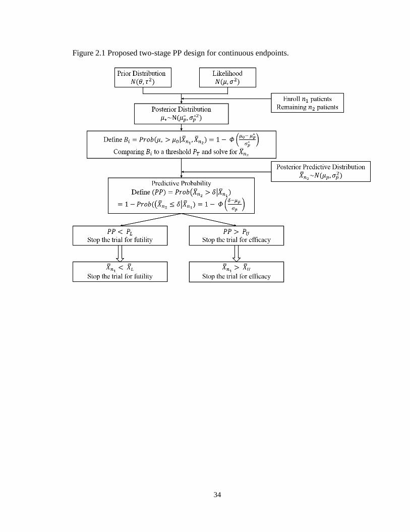
The proposed extension of Lee and Liu's PP design for continuous endpoints is

described in Figure 2.1. For notation purposes, we define the percentage decrease in the

sum of the longest diameter of the target lesions compared to baseline as “tumor size

change” and assume it is normally distributed with mean 𝜇 and variance 𝜎2, where 𝜎2 is

assumed to be known. Positive values of 𝜇 represent shrinkage in the tumor size. We

choose a normal conjugate prior distribution 𝑁(𝜃, 𝜏2) for 𝜇 , which represents the

investigator’s previous knowledge of the tumor size change from standard treatment or

historical control. We also define the effective sample size for the prior (ESS) as 𝜎2

𝜏2,

according to previous literature [67]. ESS can be understood as the amount of information

and weight contained in the prior. We set the maximum accrual of patients to 𝑁𝑚𝑎𝑥. The

number of patients in the first stage is 𝑛1 and in the second stage is 𝑛2, where 𝑛1 + 𝑛2 =

𝑁𝑚𝑎𝑥. After recruiting 𝑛1 patients in the first stage, the mean percentage change of the

tumor size from these 𝑛1 patients is denoted as �̅�𝑛1 . Thus, the corresponding posterior

distribution on 𝜇 is normally distributed with

𝐸(𝜇|𝑥1, 𝑥2, … , 𝑥𝑛1) = 𝜎2𝜃

𝑛1𝜏2 + 𝜎2+

𝑛1𝜏2

𝑛1𝜏2 + 𝜎2�̅�𝑛1

𝑉𝑎𝑟(𝜇|𝑥1, 𝑥2, … , 𝑥𝑛1) = 𝜏2𝜎2

𝑛1𝜏2 + 𝜎2

20

Further, if we were to observe the future 𝑛2 patients, the new posterior distribution of the

tumor size change, 𝜇∗, follows a normal distribution with the mean 𝜇𝑝∗ and 𝜎𝑝

∗2, where

𝜇𝑝∗ =

𝜎2𝜃

(𝑛1 + 𝑛2)𝜏2 + 𝜎2+

𝑛1𝜏2

(𝑛1 + 𝑛2)𝜏2 + 𝜎2�̅�𝑛1 +

𝑛2𝜏2�̅�𝑛2

(𝑛1 + 𝑛2)𝜏2 + 𝜎2

𝜎𝑝∗2 =

𝜏2𝜎2

(𝑛1 + 𝑛2)𝜏2 + 𝜎2

Similar to Lee and Liu's PP design, we define 𝐵𝑖 = 𝑃𝑟𝑜𝑏(𝜇∗ > 𝜇0|�̅�𝑛1 , �̅�𝑛2). 𝐵𝑖 measures

the probability that the mean tumor size change is larger than 𝜇0, given the mean tumor

size change in current 𝑛1 patients and future 𝑛2 patients. Comparing 𝐵𝑖 to a threshold 𝑃𝑇,

we aim to conclude the treatment is efficacious when 𝐵𝑖 > 𝑃𝑇,

𝐵𝑖 = 𝑃𝑟𝑜𝑏(𝜇∗ > 𝜇0|�̅�𝑛1 , �̅�𝑛2) = 1 − 𝑃𝑟𝑜𝑏(𝜇∗ ≤ 𝜇0|�̅�𝑛1 , �̅�𝑛2)

= 1 − 𝛷 (𝜇0− 𝜇𝑝

∗

𝜎𝑝∗ ) > 𝑃𝑇

where 𝛷 (.) represents the cumulative density function (CDF) of the standard normal

distribution. The above inequality (1) can be derived into an inequality of �̅�𝑛2 regarding

𝑃𝑇.

�̅�𝑛2 >((𝑛1 + 𝑛2)𝜏

2 + 𝜎2) (𝜇0 − 𝜎𝑝∗𝛷−1(1 − 𝑃𝑇)) − 𝜎

2𝜃 − 𝜏2𝑛1�̅�𝑛1

𝑛2𝜏2= 𝛿

The posterior predictive distribution of tumor size change from the future 𝑛2 patients

follows a normal distribution 𝑁(𝜇𝑝, 𝜎𝑝2), where

𝜇𝑝 = 𝜎2𝜃

𝑛1𝜏2 + 𝜎2+

𝑛1𝜏2

𝑛1𝜏2 + 𝜎2�̅�𝑛1

(1)

(2)

21

𝜎𝑝2 =

𝜎2

𝑛2+

𝜏2𝜎2

𝑛1𝜏2 + 𝜎2

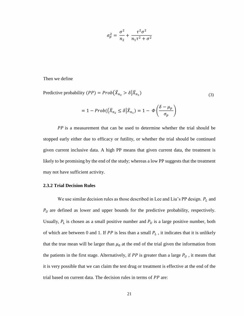
Then we define

Predictive probability (𝑃𝑃) = 𝑃𝑟𝑜𝑏(�̅�𝑛2 > 𝛿|�̅�𝑛1)

= 1 − 𝑃𝑟𝑜𝑏((�̅�𝑛2 ≤ 𝛿|�̅�𝑛1) = 1 − 𝛷 (𝛿 − 𝜇𝑝

𝜎𝑝)

𝑃𝑃 is a measurement that can be used to determine whether the trial should be

stopped early either due to efficacy or futility, or whether the trial should be continued

given current inclusive data. A high PP means that given current data, the treatment is

likely to be promising by the end of the study; whereas a low PP suggests that the treatment

may not have sufficient activity.

2.3.2 Trial Decision Rules

We use similar decision rules as those described in Lee and Liu’s PP design. 𝑃𝐿 and

𝑃𝑈 are defined as lower and upper bounds for the predictive probability, respectively.

Usually, 𝑃𝐿 is chosen as a small positive number and 𝑃𝑈 is a large positive number, both

of which are between 0 and 1. If 𝑃𝑃 is less than a small 𝑃𝐿 , it indicates that it is unlikely

that the true mean will be larger than 𝜇0 at the end of the trial given the information from

the patients in the first stage. Alternatively, if 𝑃𝑃 is greater than a large 𝑃𝑈 , it means that

it is very possible that we can claim the test drug or treatment is effective at the end of the

trial based on current data. The decision rules in terms of 𝑃𝑃 are:

(3)

22

If 𝑃𝑃 < 𝑃𝐿, stop the trial early for futility;

If 𝑃𝑃 > 𝑃𝑈, stop the trial early for efficacy;

Otherwise, continue to enroll patients to the next stage.

By comparing 𝑃𝑃 with 𝑃𝐿 and 𝑃𝑈 and solving for �̅�𝑛1, we can obtain �̅�𝐿 and �̅�𝑈,

which are defined as the lower and upper bounds for the sample mean from patients in

the first stage , �̅�𝑛1, respectively.

�̅�𝐿 =

𝑘1𝑘2𝜇0 − 𝑘1𝑘2𝜎𝑝∗𝛷−1(1 − 𝑃𝑇) − 𝑛2𝜏

2𝑘2(𝜎𝑝𝛷−1(1 − 𝑃𝐿))

𝑘2 + 𝑛2𝜏2− 𝜎2𝜃

𝑛1𝜏2

�̅�𝑈 =

𝑘1𝑘2𝜇0 − 𝑘1𝑘2𝜎𝑝∗𝛷−1(1 − 𝑃𝑇) − 𝑛2𝜏

2𝑘2 (𝜎𝑝𝛷−1(1 − 𝑃𝑈))

𝑘2 + 𝑛2𝜏2− 𝜎2𝜃

𝑛1𝜏2

where 𝑘1 = (𝑛1 + 𝑛2)𝜏2 + 𝜎2, 𝑘2 = 𝑛1𝜏

2 + 𝜎2.

Thus, in our design, the decision rule can equivalently be described as follows in terms of

�̅�𝐿 and �̅�𝑈:

If �̅�𝑛1 < �̅�𝐿 , stop the trial at the end of the first stage for futility, reject the

alternative hypothesis and claim the treatment is not promising;

If �̅�𝑛1 > �̅�𝑈, stop the trial at the end of the first stage for efficacy, reject the null

hypothesis and claim the study therapy is promising;

Otherwise, if �̅�𝐿 ≤ �̅�𝑛1 ≤ �̅�𝑈 continues to the second stage with additional 𝑛2

patients.

(4)

(5)

23

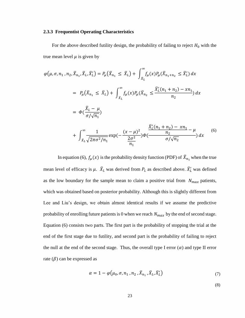
2.3.3 Frequentist Operating Characteristics

For the above described futility design, the probability of failing to reject 𝐻0 with the

true mean level 𝜇 is given by

𝜑(𝜇, 𝜎, 𝑛1 , 𝑛2, �̅�𝑛1 , �̅�𝐿 , �̅�𝐿′) = 𝑃𝜇(�̅�𝑛1 ≤ �̅�𝐿) + ∫ 𝑓𝜇(𝑥)𝑃𝜇(�̅�𝑛1+𝑛2 ≤ �̅�𝐿

′)∞

�̅�𝐿

𝑑𝑥

= 𝑃𝜇(�̅�𝑛1 ≤ �̅�𝐿) + ∫ 𝑓𝜇(𝑥)𝑃𝜇(�̅�𝑛2 ≤�̅�𝐿′(𝑛1 + 𝑛2) − 𝑥𝑛1

𝑛2)

∞

�̅�𝐿

𝑑𝑥

= 𝛷(�̅�𝐿 − 𝜇

𝜎/√𝑛1)

+ ∫1

√2𝜋𝜎2/𝑛1exp (−

(𝑥 − 𝜇)2

2𝜎2

𝑛1

)𝛷(

�̅�𝐿′(𝑛1 + 𝑛2) − 𝑥𝑛1

𝑛2− 𝜇

𝜎/√𝑛2)

∞

�̅�𝐿

𝑑𝑥

In equation (6), 𝑓𝜇(𝑥) is the probability density function (PDF) of �̅�𝑛1 when the true

mean level of efficacy is 𝜇. �̅�𝐿 was derived from 𝑃𝐿 as described above. �̅�𝐿′ was defined

as the low boundary for the sample mean to claim a positive trial from 𝑁𝑚𝑎𝑥 patients,

which was obtained based on posterior probability. Although this is slightly different from

Lee and Liu’s design, we obtain almost identical results if we assume the predictive

probability of enrolling future patients is 0 when we reach 𝑁𝑚𝑎𝑥 by the end of second stage.

Equation (6) consists two parts. The first part is the probability of stopping the trial at the

end of the first stage due to futility, and second part is the probability of failing to reject

the null at the end of the second stage. Thus, the overall type I error (𝛼) and type II error

rate (𝛽) can be expressed as

𝛼 = 1 − 𝜑(𝜇0, 𝜎, 𝑛1 , 𝑛2 , �̅�𝑛1 , �̅�𝐿 , �̅�𝐿′) (7)

(8)

(6)

24

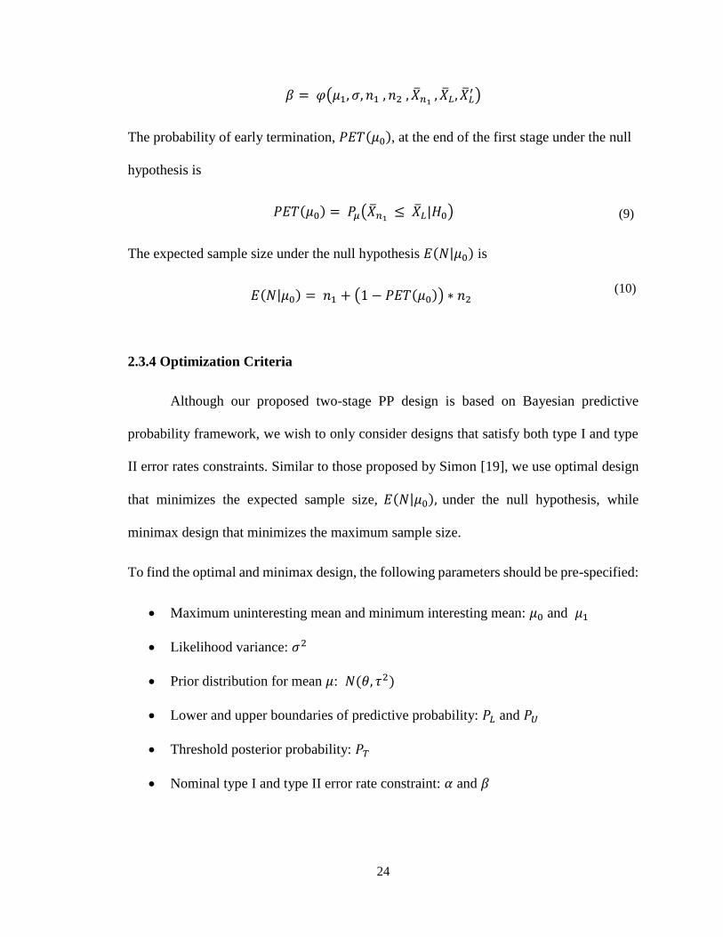
𝛽 = 𝜑(𝜇1, 𝜎, 𝑛1 , 𝑛2 , �̅�𝑛1 , �̅�𝐿 , �̅�𝐿′)

The probability of early termination, 𝑃𝐸𝑇(𝜇0), at the end of the first stage under the null

hypothesis is

𝑃𝐸𝑇(𝜇0) = 𝑃𝜇(�̅�𝑛1 ≤ �̅�𝐿|𝐻0)

The expected sample size under the null hypothesis 𝐸(𝑁|𝜇0) is

𝐸(𝑁|𝜇0) = 𝑛1 + (1 − 𝑃𝐸𝑇(𝜇0)) ∗ 𝑛2

2.3.4 Optimization Criteria

Although our proposed two-stage PP design is based on Bayesian predictive

probability framework, we wish to only consider designs that satisfy both type I and type

II error rates constraints. Similar to those proposed by Simon [19], we use optimal design

that minimizes the expected sample size, 𝐸(𝑁|𝜇0), under the null hypothesis, while

minimax design that minimizes the maximum sample size.

To find the optimal and minimax design, the following parameters should be pre-specified:

Maximum uninteresting mean and minimum interesting mean: 𝜇0 and 𝜇1

Likelihood variance: 𝜎2

Prior distribution for mean 𝜇: 𝑁(𝜃, 𝜏2)

Lower and upper boundaries of predictive probability: 𝑃𝐿 and 𝑃𝑈

Threshold posterior probability: 𝑃𝑇

Nominal type I and type II error rate constraint: 𝛼 and 𝛽

(9)

(10)

25

𝑃𝐿 , 𝑃𝑈 and 𝑃𝑇 should be between 0 and 1. When we want to stop the trial early

only for futility, we chose 𝑃𝑈 = 1.0 not to allow early stopping for efficacy since there are

situations when the treatment is beneficial for patients, there is little reason to stop the trial

early. In addition, it will help gain more precision for the estimation of clinical endpoints

of interest and provide more information for future large trials. 𝑃𝑇 is usually a large positive

constant between 0 and 1, in this paper, we set the searching range for 𝑃𝑇 as [0.9 - 0.99].

𝑃𝐿 is usually a small positive constant, which we set as [0.001 – 0.1] for the searching range

in this study. How to choose 𝑃𝑇 and 𝑃𝐿 as well as their impact stopping rules will be

discussed in Section 4. By searching over all possible values of in the range of 𝑃𝐿 and 𝑃𝑇,

the goal is to identify the combinations of 𝑃𝐿 and 𝑃𝑇 to yield the desirable power within

the constraint of the specified type I error rates. The sample size from single-stage trial for

continuous variables was used to derive the searching range for 𝑁𝑚𝑎𝑥 . Although a bit

arbitrary, if we denote 𝑁 as the sample size required for the single-stage design, we used

the range from 0.7𝑁 𝑡𝑜 1.7𝑁 to search for 𝑁𝑚𝑎𝑥. According to our simulation experiences,

this range covers almost all the situations. Therefore, by varying 𝑛1 and 𝑁𝑚𝑎𝑥 from small

to large, the design with the smallest expected sample size under the null hypothesis, that

controls both type I and type II error rates at the nominal level, is defined the optimal design.

Similarly, the design with the smallest 𝑁𝑚𝑎𝑥 is defined as the minimax design.

2.4 Results

Table 2.1 and Table 2.2 illustrate both optimal and minimax two-stage designs

which only allows early termination for futility. The tabulated results vary by effect size

(1, 0.8, 0.5 and 0.2). The effect size, also referred as to Cohen’s d, is defined as (𝜇1 −

26

𝜇0)/σ, where 𝜇0 and 𝜇1 are the average tumor size change under null and alternative

hypothesis, respectively [68]. We chose 0.2, 0.5, 0.8 and 1 to cover the range of possibilities

of small, medium and large effect sizes. We also provided other effect sizes from 0.1 to 0.9

in the appendices (Table A3.1-3.4). Table 2.1 and Table 2.2 display 𝑃𝐿, 𝑃𝑇, total sample

size from two-stages 𝑁𝑚𝑎𝑥, sample size for the first stage 𝑛1, the upper boundary of the

reject region at the end of the first stage �̅�𝐿 and the upper boundary of the reject region at

the end of the second stage �̅�𝐿,. Following Lee and Liu’s definition, the reject region was

the outcome space leading to the rejection of the new treatment/agent. The probability of

early termination (PET), expected total sample size under the null hypothesis (𝐸𝑛) and

actual type I and II error rates are also reported.

In this scenario, we assume an average of 20% tumor size shrinkage after standard

treatment or from historical control, and we wish to test if the new treatment or agent will

improve the shrinkage to 30%. Thus, the null hypothesis is 𝐻0 : 𝜇 ≤ 20% and the

alternative hypothesis is 𝐻𝐴: 𝜇 ≥ 30%, where 𝜇0 = 20 and 𝜇1 = 30. Positive values of the

parameter favor the new drug efficacy, whereas negative values represent the disease

progression. We chose various 𝜎 (10, 12.5, 20 and 50) to compare the sample size for

different effect sizes, where in practice, 𝜎 should be obtained from historical trials or

estimated from standard treatment. We set ESS = 𝜎2

𝜏2= 1 and 𝜃 = 𝜇0 = 20. As described

above, the searching range for 𝑁𝑚𝑎𝑥 was obtained from a single-stage trial with continuous

endpoints. A grid search was performed through the space of 𝑃𝐿 [0.001 – 0.1] and 𝑃𝑇[0.9

– 0.99] to enumerate all the combinations that meet pre-specified type I and type II error

constraints.

27

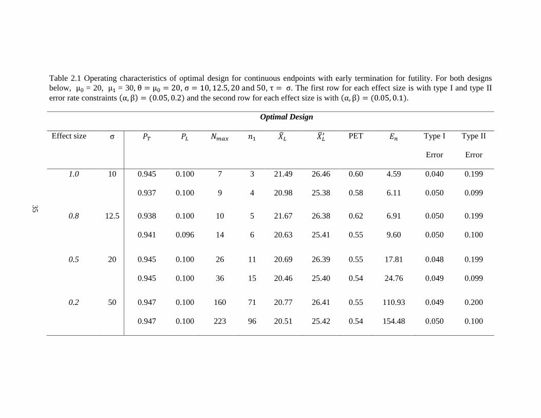
For instance, in Table 2.1, when 𝜎 = 20 with effect size 0.5, type I and type II error

rate constraints are 0.05 and 0.2, a grid search of 𝑃𝐿 and 𝑃𝑇 was performed for each 𝑁𝑚𝑎𝑥

between 8 and 46. It turns out that the design with 11 patients in the first stage and 26

patients in total is the optimal design, which has the smallest expected sample under the

null hypothesis. 𝑃𝐿 and 𝑃𝑇 are determined to be 0.1 and 0.945, respectively. The trial will

be stopped, and the new drug is considered not promising for further study when the

average tumor size shrinkage from the first 11 patients is less than 20.69%. If the observed

value of the mean of tumor size shrinkage from the first 11 patients is greater than 20.69%,

the trial should continue to the second stage and enroll an additional 15 patients. The

expected total sample size is 17.8, and the probability of early termination is 0.55 when the

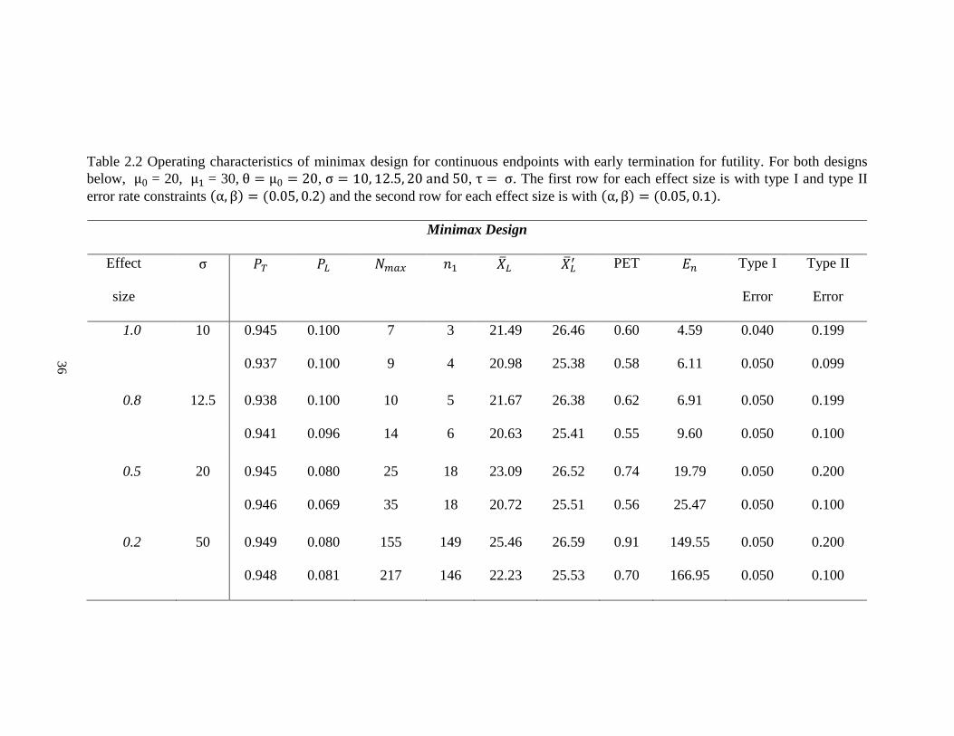
true mean tumor size change is 20%. Alternatively, the minimax design requires 25 patients

in total with 18 patients in the first stage (Table 2.2). In fact, the minimax design usually

gives a smaller total sample size but larger 𝑛1, �̅�𝑛1, 𝐸𝑛 and PET. This trend is consistent

with both Simon’s and Hsiao’s designs [19, 56]. As expected, the total sample size required

decreases as effect size increases.

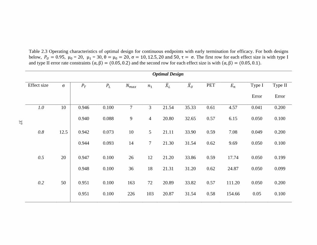
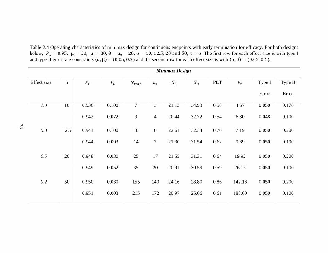
Table 2.3 and 2.4 display the optimal designs and minimax designs, which allow

early termination due to either futility or efficacy. In both designs, we use 𝑃𝑈 = 0.95 to

make the efficacy stopping decision. Using the same example, when 𝜎 = 20 with effect

size 0.5, type I and type II error rate constraints are 0.05 and 0.2, the optimal design yields

the same total sample 26 with 12 patients required for the first stage (Table 2.3). The trial

will be stopped and the new drug is considered not promising for further study when the

average tumor size shrinkage from the first 11 patients is less than 21.20%. If the observed

value of the mean of tumor size shrinkage from the first 11 patients is greater than 33.86%,

28

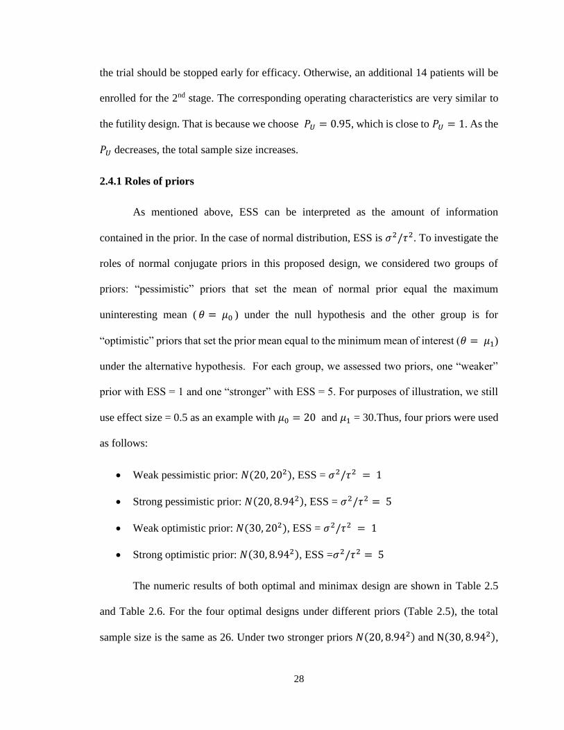
the trial should be stopped early for efficacy. Otherwise, an additional 14 patients will be

enrolled for the 2nd stage. The corresponding operating characteristics are very similar to

the futility design. That is because we choose 𝑃𝑈 = 0.95, which is close to 𝑃𝑈 = 1. As the

𝑃𝑈 decreases, the total sample size increases.

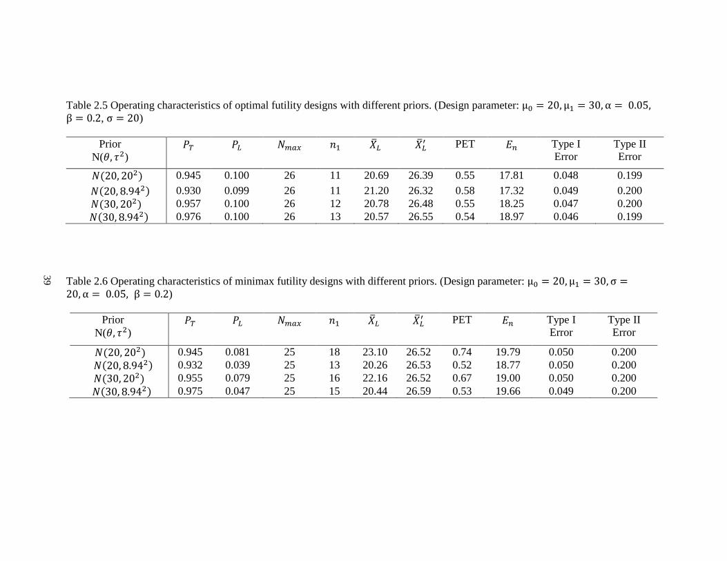
2.4.1 Roles of priors

As mentioned above, ESS can be interpreted as the amount of information

contained in the prior. In the case of normal distribution, ESS is 𝜎2/𝜏2. To investigate the

roles of normal conjugate priors in this proposed design, we considered two groups of

priors: “pessimistic” priors that set the mean of normal prior equal the maximum

uninteresting mean ( 𝜃 = 𝜇0 ) under the null hypothesis and the other group is for

“optimistic” priors that set the prior mean equal to the minimum mean of interest (𝜃 = 𝜇1)

under the alternative hypothesis. For each group, we assessed two priors, one “weaker”

prior with ESS = 1 and one “stronger” with ESS = 5. For purposes of illustration, we still

use effect size = 0.5 as an example with 𝜇0 = 20 and 𝜇1 = 30.Thus, four priors were used

as follows:

Weak pessimistic prior: 𝑁(20, 202), ESS = 𝜎2/𝜏2 = 1

Strong pessimistic prior: 𝑁(20, 8.942), ESS = 𝜎2/𝜏2 = 5

Weak optimistic prior: 𝑁(30, 202), ESS = 𝜎2/𝜏2 = 1

Strong optimistic prior: 𝑁(30, 8.942), ESS =𝜎2/𝜏2 = 5

The numeric results of both optimal and minimax design are shown in Table 2.5

and Table 2.6. For the four optimal designs under different priors (Table 2.5), the total

sample size is the same as 26. Under two stronger priors 𝑁(20, 8.942) and N(30, 8.942),

29

the strong optimistic prior N(30, 8.942) results in a larger expected sample size of 18.97

under the null hypothesis, compared to 17.32 from the strong pessimistic prior

𝑁(20, 8.942). It is intuitive since the trial is less likely to be terminated early due to futility

under the null hypothesis if the optimistic prior belief is true (PET = 0.58 for prior

𝑁(20, 8.942) vs. PET = 0.54 for prior 𝑁(30, 8.942)). Under two weaker priors 𝑁(20, 202)

and 𝑁(30, 202), the PET is the same but the optimistic prior also leads to a larger expected

sample size of (18.25 vs. 17.81) under the null hypothesis. When comparing the minimax

design (Table 2.6), all the four priors resulted in the sample maximum sample size (𝑁 =

25). The two weaker priors need a larger sample size from the first stage n1 than the

stronger priors.

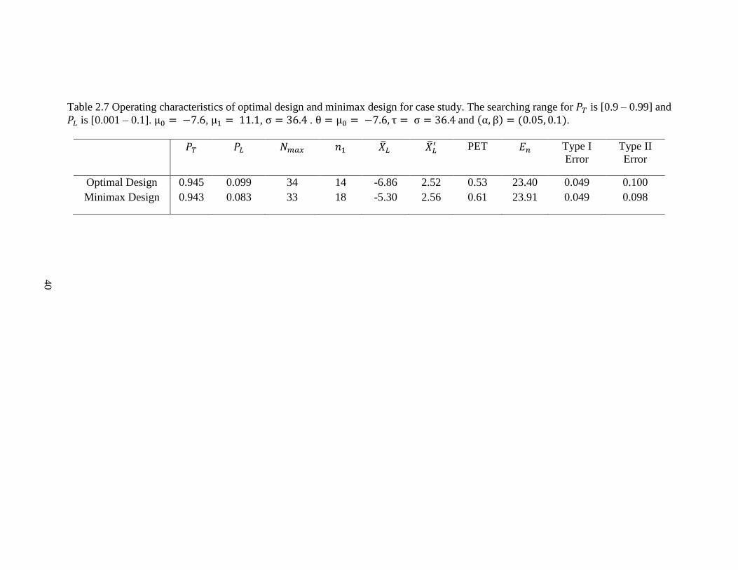
2.4.2 Case Study

In this section, we refer to the case study illustrated in Wason et al. [5]. In this case

study, the primary endpoint was the maximum shrinkage in total lesion diameter and was

previously classified as a binary variable according to RECIST criteria. Thus, the trial was

previously designed using a Simon’s two-stage design. In their proposed two-stage design,

Wason et al. demonstrated that using continuous endpoints, instead of classified binary

endpoints, there was about 50% reduction in both expected and maximum sample size.

According to their notation, the mean treatment efficacy (true tumor shrinkage) was

denoted by 𝛿. The hypothesis testing framework was 𝐻0: 𝜇 ≤ 𝜇0 vs. 𝐻1: 𝜇 ≥ 𝜇1, where

𝜇0 = −7.6 and 𝜇1 = 11.1, with known 𝜎 = 36.4. Under this setup, Wason’s optimal

continuous design yielded a first and second stage sample size of 15 and 24, respectively,

which compared with Simon’s two-stage optimal design (30 patients are required for the

30

first stage and 52 patients were required for the second stage), led to around 50% reduction

in the sample size for both stages.

We apply our Bayesian PP design for this trial scenario. In particular, 𝜇0 = −7.6,

𝜇1 = 11.1, and 𝜎 = 36.4. We chose the prior as 𝑁(−7.6, 36.42) and set the same type I

and II error rates as 0.05 and 0.1, respectively. The searching range for 𝑃𝐿 is [0.001 - 0.1]

and for 𝑃𝑇 is [0.9 - 0.99]. These values result in the optimal continuous design having the

first stage sample size of 14 and total sample size of 34. The expected sample size under

the null is 23.4. The cut-off value for tumor size change from the first 14 patients is -6.86,

with 𝑃𝑇 = 0.945 and 𝑃𝐿 = 0.099 (Table 2.7). The result is very similar to Wason et al., but

requires a slightly smaller sample size in the second stage.

2.5 Discussion

In practice, RECIST criteria is commonly applied to categorize the tumor shrinkage

into complete response, partial response, progressive disease, and stable disease. Response

rate, which is the combination of complete and partial response, with at least a 30%

decrease in the sum of the longest diameter of the target lesions, is usually used as a

secondary endpoint in most of the cancer trials. However, as shown in the previous studies,

this dichotomization not only lead to loss of statistical efficiency, but greatly increases the

required sample size [5, 54, 56].

In this proposed design, we extended Lee and Liu’s predictive probability approach

into a two-stage setting for continuous endpoint. Similar as Wason et al., we obtained

decreased sample size when treating tumor shrinkage as continuous variable. The design

parameters 𝑃𝐿 , 𝑃𝑈 , and 𝑃𝑇 plays an important role in searching for the optimal and

31

minimax designs. As mentioned above, we chose 𝑃𝑈 = 1 to only allow for early futility

stopping. Regarding the choice of 𝑃𝐿, 𝑃𝑈, and 𝑃𝑇, no definitive and clear guidelines have

been proposed for the binary endpoints. We adopted similar strategy as described in Lee

and Liu’s paper and Dong et al’s research [37, 39]. We set the range of 𝑃𝑇 for searching

as [0.9 - 0.99]. 𝑃𝑇 can be viewed as a reasonable degree of certainty, which could be 0.9,

0.95 and 0.99, according to FDA guidelines for the use Bayesian statistics in medical

device clinical trials [39, 69]. The lower boundary for 𝜃𝑇 can be reduced to 0.8, as Lee and

Liu did in their binary PP design. In general, as 𝑃𝑇 increases, it is harder to reject 𝐻0.

Therefore, the higher 𝜃𝑇 is, the lower power and actual type I error it will be. There is no

general guideline for choosing 𝑃𝐿. Lee and Liu set the search range for 𝑃𝐿 as [0.001 - 0.1],

while Dong et al. used values up to 𝑃𝐿 = 0.5 [39]. We applied the same rule as Lee and Liu,

since a smaller value of 𝑃𝐿 indicates that it is very unlikely the mean tumor size change

will be larger than 𝜇0 given current information, which turns into harder rejection of 𝐻0

due to futility as well as increased power and type I error rates.

We also assessed the operating characteristics for the optimal designs based on the

posterior approach. Our simulation results have shown that a two-stage design based on

the posterior approach is more conservative, and always yields a little bit larger total sample

size 𝑁𝑚𝑎𝑥 and larger �̅�𝑛1 (data not shown). For instance, if we use posterior probability

approach for the case study, the �̅�𝑛1 is -2.59, and we need 39 patients in total with 15

patients for the first stage, which happened to be the same as Wason’s design. However,

as mentioned in Lee and Liu’ s paper, predictive probability approach has the advantages

that it mimics the decision making process in reality and more intuitive [37].

32

We explored and evaluated the roles of priors for this PP design. In practice, prior

information is usually obtained from standard treatment or historical control. ESS

represents the weight we place on the prior information known before the trial. In this paper,

we began with ESS = 1, assuming a weak prior. The total sample size remains robust with

stronger priors (ESS = 5) for both optimal and minimax designs. The comparison is

illustrative but not conclusive. Based on our simulation, ESS should not exceed 1/3 of the

total sample size. Future work on the exploration of other non-conjugated priors is needed.

There are several limitations to this current design that we plan to address in future

work. Firstly, in this proposed design, we assume the standard deviation 𝜎 is known in line

with Wason’s design. It is reasonable since in practice, this value could be obtained from

previous trials or preclinical studies. However, when there is little prior information

available, especially for novel drugs or biomarkers, unknown variance may be explored in

the future. Secondly, this design currently accommodates only one interim look for futility,

and we plan to eventually incorporate continuously monitoring for both futility and

superiority. Further, priors are important in Bayesian clinical trial designs. It is always

challenging and controversial to choose a suitable prior on the parameter of interest. In this

paper, we only chose the conjugate priors for the mean, assuming variance is known, and

explored briefly on the roles of pessimistic and optimistic priors. There could be clinical

situations where the prior does not follow a normal distribution, and thus the resulting

posterior does not have a closed form. More exploration is needed in this regard.

Overall, we have shown a two-stage design using predictive probability for

continuous endpoints. We have demonstrated similar sample size reduction as Wason’s

design. We developed R programs to perform this proposed design and the code will be

33

available in an upcoming R package, but these functions are available upon request. As

research rapidly moves to incorporate more immunotherapies and targeted therapies, these

designs will accommodate new types of outcomes while allowing for flexible stopping

rules for futility and/or efficacy to continue optimizing trial resources and prioritizing

agents with compelling early phase data.

34

Figure 2.1 Proposed two-stage PP design for continuous endpoints.

35

Table 2.1 Operating characteristics of optimal design for continuous endpoints with early termination for futility. For both designs

below, μ0 = 20, μ1 = 30, θ = μ0 = 20, σ = 10, 12.5, 20 and 50, τ = σ. The first row for each effect size is with type I and type II

error rate constraints (α, β) = (0.05, 0.2) and the second row for each effect size is with (α, β) = (0.05, 0.1).

Optimal Design

Effect size σ 𝑃𝑇 𝑃𝐿 𝑁𝑚𝑎𝑥 𝑛1 �̅�𝐿 �̅�𝐿′ PET 𝐸𝑛 Type I

Error

Type II

Error

1.0 10 0.945 0.100 7 3 21.49 26.46 0.60 4.59 0.040 0.199

0.937 0.100 9 4 20.98 25.38 0.58 6.11 0.050 0.099

0.8 12.5 0.938 0.100 10 5 21.67 26.38 0.62 6.91 0.050 0.199

0.941 0.096 14 6 20.63 25.41 0.55 9.60 0.050 0.100

0.5 20 0.945 0.100 26 11 20.69 26.39 0.55 17.81 0.048 0.199

0.945 0.100 36 15 20.46 25.40 0.54 24.76 0.049 0.099

0.2 50 0.947 0.100 160 71 20.77 26.41 0.55 110.93 0.049 0.200

0.947 0.100 223 96 20.51 25.42 0.54 154.48 0.050 0.100

36

Table 2.2 Operating characteristics of minimax design for continuous endpoints with early termination for futility. For both designs

below, μ0 = 20, μ1 = 30, θ = μ0 = 20, σ = 10, 12.5, 20 and 50, τ = σ. The first row for each effect size is with type I and type II

error rate constraints (α, β) = (0.05, 0.2) and the second row for each effect size is with (α, β) = (0.05, 0.1).

Minimax Design

Effect

size

σ 𝑃𝑇 𝑃𝐿 𝑁𝑚𝑎𝑥 𝑛1 �̅�𝐿 �̅�𝐿′ PET 𝐸𝑛 Type I

Error

Type II

Error

1.0 10 0.945 0.100 7 3 21.49 26.46 0.60 4.59 0.040 0.199

0.937 0.100 9 4 20.98 25.38 0.58 6.11 0.050 0.099

0.8 12.5 0.938 0.100 10 5 21.67 26.38 0.62 6.91 0.050 0.199

0.941 0.096 14 6 20.63 25.41 0.55 9.60 0.050 0.100

0.5 20 0.945 0.080 25 18 23.09 26.52 0.74 19.79 0.050 0.200

0.946 0.069 35 18 20.72 25.51 0.56 25.47 0.050 0.100

0.2 50 0.949 0.080 155 149 25.46 26.59 0.91 149.55 0.050 0.200

0.948 0.081 217 146 22.23 25.53 0.70 166.95 0.050 0.100

37

Table 2.3 Operating characteristics of optimal design for continuous endpoints with early termination for efficacy. For both designs

below, 𝑃𝑈 = 0.95, μ0 = 20, μ1 = 30, θ = μ0 = 20, σ = 10, 12.5, 20 and 50, τ = σ. The first row for each effect size is with type I

and type II error rate constraints (α, β) = (0.05, 0.2) and the second row for each effect size is with (α, β) = (0.05, 0.1).

Optimal Design

Effect size σ 𝑃𝑇 𝑃𝐿 𝑁𝑚𝑎𝑥 𝑛1 �̅�𝐿 �̅�𝑈 PET 𝐸𝑛 Type I

Error

Type II

Error

1.0 10 0.946 0.100 7 3 21.54 35.33 0.61 4.57 0.041 0.200

0.940 0.088 9 4 20.80 32.65 0.57 6.15 0.050 0.100

0.8 12.5 0.942 0.073 10 5 21.11 33.90 0.59 7.08 0.049 0.200

0.944 0.093 14 7 21.30 31.54 0.62 9.69 0.050 0.100

0.5 20 0.947 0.100 26 12 21.20 33.86 0.59 17.74 0.050 0.199

0.948 0.100 36 18 21.31 31.20 0.62 24.87 0.050 0.099

0.2 50 0.951 0.100 163 72 20.89 33.82 0.57 111.20 0.050 0.200

0.951 0.100 226 103 20.87 31.54 0.58 154.66 0.05 0.100

38

Table 2.4 Operating characteristics of minimax design for continuous endpoints with early termination for efficacy. For both designs

below, 𝑃𝑈 = 0.95, μ0 = 20, μ1 = 30, θ = μ0 = 20, σ = 10, 12.5, 20 and 50, τ = σ. The first row for each effect size is with type I

and type II error rate constraints (α, β) = (0.05, 0.2) and the second row for each effect size is with (α, β) = (0.05, 0.1).

Minimax Design

Effect size σ 𝑃𝑇 𝑃𝐿 𝑁𝑚𝑎𝑥 𝑛1 �̅�𝐿 �̅�𝑈 PET 𝐸𝑛 Type I

Error

Type II

Error

1.0 10 0.936 0.100 7 3 21.13 34.93 0.58 4.67 0.050 0.176

0.942 0.072 9 4 20.44 32.72 0.54 6.30 0.048 0.100

0.8 12.5 0.941 0.100 10 6 22.61 32.34 0.70 7.19 0.050 0.200

0.944 0.093 14 7 21.30 31.54 0.62 9.69 0.050 0.100

0.5 20 0.948 0.030 25 17 21.55 31.31 0.64 19.92 0.050 0.200

0.949 0.052 35 20 20.91 30.59 0.59 26.15 0.050 0.100

0.2 50 0.950 0.030 155 140 24.16 28.80 0.86 142.16 0.050 0.200

0.951 0.003 215 172 20.97 25.66 0.61 188.60 0.050 0.100

39

Table 2.5 Operating characteristics of optimal futility designs with different priors. (Design parameter: μ0 = 20, μ1 = 30, α = 0.05,β = 0.2, σ = 20)

Prior

N(𝜃, 𝜏2)

𝑃𝑇 𝑃𝐿 𝑁𝑚𝑎𝑥 𝑛1 �̅�𝐿 �̅�𝐿′ PET 𝐸𝑛 Type I

Error

Type II

Error

𝑁(20, 202) 0.945 0.100 26 11 20.69 26.39 0.55 17.81 0.048 0.199

𝑁(20, 8.942) 0.930 0.099 26 11 21.20 26.32 0.58 17.32 0.049 0.200

𝑁(30, 202) 0.957 0.100 26 12 20.78 26.48 0.55 18.25 0.047 0.200

𝑁(30, 8.942) 0.976 0.100 26 13 20.57 26.55 0.54 18.97 0.046 0.199

Table 2.6 Operating characteristics of minimax futility designs with different priors. (Design parameter: μ0 = 20, μ1 = 30, σ =20, α = 0.05, β = 0.2)

Prior

N(𝜃, 𝜏2)

𝑃𝑇 𝑃𝐿 𝑁𝑚𝑎𝑥 𝑛1 �̅�𝐿 �̅�𝐿′ PET 𝐸𝑛 Type I

Error

Type II

Error

𝑁(20, 202) 0.945 0.081 25 18 23.10 26.52 0.74 19.79 0.050 0.200

𝑁(20, 8.942) 0.932 0.039 25 13 20.26 26.53 0.52 18.77 0.050 0.200

𝑁(30, 202) 0.955 0.079 25 16 22.16 26.52 0.67 19.00 0.050 0.200

𝑁(30, 8.942) 0.975 0.047 25 15 20.44 26.59 0.53 19.66 0.049 0.200

40

Table 2.7 Operating characteristics of optimal design and minimax design for case study. The searching range for 𝑃𝑇 is [0.9 – 0.99] and

𝑃𝐿 is [0.001 – 0.1]. μ0 = −7.6, μ1 = 11.1, σ = 36.4 . θ = μ0 = −7.6, τ = σ = 36.4 and (α, β) = (0.05, 0.1).

𝑃𝑇 𝑃𝐿 𝑁𝑚𝑎𝑥 𝑛1 �̅�𝐿 �̅�𝐿′ PET 𝐸𝑛 Type I

Error

Type II

Error

Optimal Design 0.945 0.099 34 14 -6.86 2.52 0.53 23.40 0.049 0.100

Minimax Design 0.943 0.083 33 18 -5.30 2.56 0.61 23.91 0.049 0.098

41

CHAPTER THREE

A Multi-Stage Predictive Probability Interim Design for Phase II Clinical Trials

with Continuous Endpoints

3.1 Abstract

Numerous phase II cancer clinical trial designs are based on binary response rate

outcomes. The loss of information is particularly inefficient due to the dichotomization of

tumor shrinkage according to RECIST criteria. In this paper, we extended Lee and Liu’s

probability predictive design for binary outcomes into a single-arm multi-stage setting for

continuous endpoints, such as continuous tumor shrinkage in cancer trials or any other

short-term response endpoints. We present the numeric simulation outputs for minimax

designs with different prior distributions, while maintaining robust results. This predictive

probability design is flexible due to its Bayesian properties. It keeps updating the

information during the trial as the patients are continuously enrolled. In the meanwhile, it

also controls the frequentist type I and type II error rates. We also developed R programs

to assist with the study design.

Keywords: Multi-stage design; Predictive probability; Interim strategy; Continuous

endpoints

3.2 Introduction

Phase II clinical trials aim to screen out those ineffective treatment or therapies,

and identify those effective ones to move forward to larger confirmatory randomized phase

III trials. As a result, phase II trials tend to have shorter study periods, smaller sample sizes,

and endpoints that aim to be predictive to the definitive phase III trials. In cancer phase II

42

trials, a commonly used endpoint is objective response rate, which is dichotomized from

continuous tumor shrinkage according to RECIST [1].

Many designs have been proposed to target potential promising new therapies for

phase II trials, among which at least one interim look is usually incorporated to utilize the

information from the interim data that has already been obtained. In the setting of single

treatment regimen or one-arm design, for the purpose of evaluating the efficacy, Gehan’s

design and Simon’s two-stage design as well as Fleming’s two-stage design are still the

most widely used two-stage designs in practice [18-19,61].In some scenarios,three-stage

design and multi-stage design are preferred to two-stage designs, since they are usually

more efficient when compared to the two-stage design, especially when the effect size is

small, and total sample size required is large. A multi-stage design is more efficient to

terminate the trial early if the new therapy is not effective [20, 70]. Chen extended Simon’s

two-stage design into a three-stage design and claimed that the average sample size

reduction from two-stage to three-stage is about 10% when the null hypothesis is true [20].

Fleming proposed a multiple testing procedure for one-sample design to allow for early

termination while maintaining the statistical properties. In the randomized setting, group

sequential designs have been widely employed, with Pocock’s design and O’Brien and

Fleming’s design as two commonly used group-sequential options[62, 63].

On the other hand, Bayesian clinical trial designs have gained popularity due to

their flexibility to include sequential stoppings when compared with their frequentist

counterparts. Thall and Simon introduced a class of phase II Bayesian clinical trial designs

[28]. Tan and Machin proposed a two-stage design based on the posterior distribution [29].

Sambucini extended it into a two-stage design based on predictive distribution [30, 31].

43

Wang et al. and Dong et al. developed two Bayesian single-arm two-stage designs

incorporating both frequentist and Bayesian error rates [34, 39]. In particular, Lee and Liu

proposed a predictive probability design for single-arm trial with binary outcome to

monitor the trial continuously[37].

Although this binary endpoint is intuitive to understand and widely adopted in

practice, loss of information from the dichotomization cannot be avoided. In addition, with

the development of molecular targeted therapies and immunotherapies, drugs can be still

active and patients can benefit from those “minor response” or “mixed response”, even

though drugs do not lead to high-levels of tumor regression and do not meet the criteria of

response rates [6, 71, 72]. Therefore, using continuous tumor shrinkage instead of the

binary response rate has been proposed in previous studies [5, 53-56, 58]. However, these

designs can be extended to any continuous outcomes, for example, biomarker assessment

over time. In this paper, we extended Lee and Liu’s predictive probability design into a

single-arm setting with continuous outcome. This manuscript is organized into the

following sections. Section 3.3 details our proposed design and trial decision rules. Section

3.4 displayed the numeric results from the simulation and case study. Section 3.5 is to

discuss the strengths, limitations and future directions of current design.

3.3. Methods

3.3.1 Notation and Proposed Design

In this paper, we extend Lee and Liu’s 𝑃𝑃 design into a multi-stage design for

continuous endpoints. The hypothesis testing framework is as follows:

𝐻0: 𝜇 ≤ 𝜇0 vs. 𝐻1: 𝜇 ≥ 𝜇1

44

where 𝜇0 represents the maximum efficacy from the standard treatment or historical

control, and 𝜇1 represents a target efficacy threshold from the treatment or therapy being

studied. This extended design also meets both pre-specified Type I and Type II error rate

constraints.

For illustration purposes, we define “tumor size change” as the percentage decrease

in the sum of the longest diameter of the target lesions compared to baseline for each patient,

with positive values denoting tumor shrinkage [73]. We assume the average tumor

shrinkage, 𝑋, follows a normal distribution 𝑁( 𝜇, 𝜎2), with mean 𝜇 and known variance

𝜎2. We assume a normal conjugate prior distribution for 𝜇, 𝑁(𝜃, 𝜏2), which represents the

investigator’s previous knowledge of the tumor size change from standard treatment or

historical control. We use effective sample size for the prior (ESS), 𝜎2

𝜏2 for the normal case,

to assign the amount of information for the prior [67, 73]. For the purpose of simulation,

we set ESS = 1, assuming very little knowledge is known before the trial starts. We also

compare the effect of different ESS specifications in the results section.

Here, we consider a single-arm 𝐾 -stage design, where 𝐾 ≤ 𝑁𝑚𝑎𝑥. At the end of

𝑖𝑡ℎ stage, the number of patients enrolled in total is denoted as 𝑛𝑖, where 𝑖 = 1, 2, … , 𝐾.

We denote �̅�𝑛𝑖 as the average tumor shrinkage for the current 𝑛𝑖 patients. Therefore, given

the information from these current 𝑛𝑖 patients, the posterior distribution of the mean tumor

shrinkage 𝜇 follows a normal distribution, with mean 𝜎2𝜃

𝑛𝑖𝜏2+𝜎2

+ 𝑛𝑖𝜏

2

𝑛𝑖𝜏2+𝜎2

�̅�𝑛𝑖 and variance

𝜏2𝜎2

𝑛𝑖𝜏2+𝜎2

. Thus, the average tumor shrinkage from the future 𝑚𝑖 patients, where 𝑚𝑖 =

𝑁𝑚𝑎𝑥 − 𝑛𝑖, follows a normal distribution with mean 𝜇𝑝∗ and 𝜎𝑝

∗2, where

45

𝜇𝑝∗ =

𝜎2𝜃

(𝑚𝑖 + 𝑛𝑖)𝜏2 + 𝜎2+

𝑛𝑖𝜏2

(𝑚𝑖 + 𝑛𝑖)𝜏2 + 𝜎2�̅�𝑛𝑖 +

𝑚𝑖𝜏2�̅�𝑚𝑖

(𝑚𝑖 + 𝑛𝑖)𝜏2 + 𝜎2

𝜎𝑝∗2 =

𝜏2𝜎2

(𝑚𝑖 + 𝑛𝑖)𝜏2 + 𝜎2

We define 𝐵𝑖 = 𝑃𝑟𝑜𝑏(𝜇∗ > 𝜇0|�̅�𝑛𝑖 , �̅�𝑚𝑖) to measure the probability that the mean tumor

shrinkage is larger than 𝜇0, given the mean tumor size change in current 𝑛𝑖 patients and

future 𝑚𝑖 patients. We can conclude the treatment is efficacious when 𝐵𝑖 > 𝑃𝑇, where 𝑃𝑇

is the posterior critical value at each stage and is usually assumed to be greater than 0.8.

𝐵𝑖 = 𝑃𝑟𝑜𝑏(𝜇∗ > 𝜇0|�̅�𝑛𝑖 , �̅�𝑚𝑖) = 1 − 𝑃𝑟𝑜𝑏(𝜇∗ ≤ 𝜇0|�̅�𝑛𝑖 , �̅�𝑚𝑖)

= 1 − 𝛷 (𝜇0− 𝜇𝑝

∗

𝜎𝑝∗ ) > 𝑃𝑇

where 𝛷 (.) represents the cumulative density function (CDF) of the standard normal

distribution. The above inequality (1) can be derived into an inequality of �̅�𝑚𝑖 regarding

𝑃𝑇.

�̅�𝑚𝑖 >((𝑛𝑖+𝑚𝑖)𝜏

2+𝜎2)(𝜇0− 𝜎𝑝∗𝛷−1(1−𝑃𝑇))− 𝜎

2𝜃−𝜏2𝑛𝑖�̅�𝑛𝑖

𝑚𝑖𝜏2 = 𝛿

The posterior predictive distribution of tumor size change from the future 𝑚 patients also

follows a normal distribution 𝑁(𝜇𝑝, 𝜎𝑝2) , with 𝜇𝑝 =

𝜎2𝜃

𝑛𝑖𝜏2+𝜎2

+ 𝑛𝑖𝜏

2

𝑛𝑖𝜏2+𝜎2

�̅�𝑛𝑖 and 𝜎𝑝2 =

𝜎2

𝑚𝑖+

𝜏2𝜎2

𝑛𝑖𝜏2+𝜎2

.

Based on all the information above, we can then define the predictive probability (𝑃𝑃)

Predictive probability (𝑃𝑃) = 𝑃𝑟𝑜𝑏(�̅�𝑚𝑖 > 𝛿|�̅�𝑛𝑖)

= 1 − 𝑃𝑟𝑜𝑏(�̅�𝑚𝑖 ≤ 𝛿|�̅�𝑛𝑖) = 1 − 𝛷 (𝛿 − 𝜇𝑝

𝜎𝑝)

(1)

(2)

(3)

46

A high 𝑃𝑃 means that given current data, the treatment is likely to be efficacious by the

end of the study; whereas a low 𝑃𝑃 suggests that the treatment may not have sufficient

activity. Therefore, we use 𝑃𝑃 to make the decision during the interims in the trial.

3.3.2 Trial Decision Rules

For this proposed design, we have the flexibility to stop the trial early either due to

futility and superiority. We use similar decision rules as those described in Lee and Liu’s

𝑃𝑃 design and our two-stage design [37, 73]. For a K-stage design (𝐾 < 𝑁𝑚𝑎𝑥), we denote

𝑃𝑃𝑖 as the predictive probability at the end of 𝑖𝑡ℎ stage (𝑖 ≤ 𝐾). We also denote 𝑃𝐿 and 𝑃𝑈

as the lower and upper boundaries for 𝑃𝑃𝑖, assuming 𝑃𝐿 and 𝑃𝑈 are constant for each stage.

𝑃𝐿 and 𝑃𝑈 should be both between 0 and 1, where 𝑃𝐿 is usually a small positive number

less than 0.1 and 𝑃𝑈 is usually a large number greater than 0.9. By comparing 𝑃𝑃𝑖 with 𝑃𝐿

and 𝑃𝑈 and solving for �̅�𝑛𝑖, we can obtain �̅�𝐿𝑖 and �̅�𝑈𝑖, which are defined as the lower and

upper bounds for the sample mean from current 𝑛𝑖 patients. Therefore, for a 𝐾-stage

design, the decision rule can be described in terms of �̅�𝐿𝑖 and �̅�𝑈𝑖 at each stage:

If �̅�𝑛𝑖 < �̅�𝐿𝑖, stop the trial for futility and reject the alternative hypothesis;

If �̅�𝑛𝑖 > �̅�𝑈𝑖, stop the trial for efficacy and reject the null hypothesis;

Otherwise, if �̅�𝐿𝑖 ≤ �̅�𝑛𝑖 ≤ �̅�𝑈𝑖, continue to the next stage.

3.3.3 Frequentist Operating Characteristics

As we want our design to meet both pre-specified type I and type II error rate

constraints, we need to calculate the probability of rejecting the null hypothesis at each

stage. Therefore, for the design described above, we obtain the average tumor shrinkage

from the cumulative sample size of the patients at the end of each stage 𝑖, denoted as �̅�𝑛𝑖,

where �̅�𝑛𝑖 follows a normal distribution with mean 𝜇 and variance 𝜎2/𝑛𝑖 . If we

47

standardize �̅�𝑛𝑖 and transform it into a test statistics, Z𝑛𝑖 = (�̅�𝑛𝑖 − 𝜇0)/(√𝜎2/𝑛𝑖), for a

given design that continues to the end, the vector of Z = (Z𝑛1 , Z𝑛2 , … , Z𝑛𝐾) is multivariate

normally distributed with the mean (𝜇 − 𝜇0)/(√𝜎2/𝑛𝑖) and variance 1. The covariance

between Z𝑛𝑖 and Z𝑛𝑗 is √𝑛𝑖

𝑛𝑗 for 𝑛𝑖 < 𝑛𝑗 [74]. Therefore, the vector of the �̅� =

(�̅�𝑛1 , �̅�𝑛2 , … , �̅�𝑛𝐾), is assumed to follow a multivariate normal distribution, with mean 𝜇

and variance 𝜎2

𝑛𝑖(𝑖 = 1,2, . . , 𝐾). The covariance between �̅�𝑛𝑖 and �̅�𝑛𝑗 , with 𝑛𝑖 < 𝑛𝑗 , is

𝜎2/ 𝑛𝑗. The probability of rejecting 𝐻0 with the true mean 𝜇 at each stage can be expressed

as:

Pr(𝑟𝑒𝑗𝑒𝑐𝑡 𝑡ℎ𝑒 𝐻0 at stage 𝑖 )

= ∫ …�̅�𝑈1�̅�𝐿1

∫ ∫ 𝑓�̅�(�̅�𝑛1 , �̅�𝑛2 , … , �̅�𝑛𝑖|𝜇)∞

�̅�𝑈𝑖

�̅�𝑈𝑖−1�̅�𝐿𝑖−1

𝑑�̅�𝑛𝑖𝑑�̅�𝑛𝑖−1

…𝑑�̅�𝑛1 ,

where 𝑓�̅� is the probability density function (pdf) of the multivariate normal distribution

with mean vector and covariance matrix as previously described. �̅�𝑈𝑖 and �̅�𝐿𝑖 are

boundaries obtained from predictive probabilities 𝑃𝐿 and 𝑃𝑈 at each stage 𝑖. When the trial

continues to the last stage 𝐾, �̅�𝑈𝐾 and �̅�𝐿𝐾 are obtained from the posterior probability. In

the two-stage paper, we compare the results with the scenario, in which we assume the

predictive probability of enrolling future patients is 0 when we reach 𝑁𝑚𝑎𝑥. It has been

shown to be very similar in the two scenarios. Therefore, the type I error and power can be

calculated by summing up the probability of rejecting the null hypothesis at each stage

when the null and alternative hypothesis is true, respectively [55].

To evaluate the multidimensional integral in the equation above, wo strategies are

applied. One directly integrates the multivariate normal density [75, 76]. Computation time

(4)

48

for the direct numeric integration is much less when the design only contains 3 or fewer

stages. Thus, we utilize a published R package, which contains a function to perform a

Monte Carlo algorithm and evaluate the integrand for 4 or more desired stages, as the

computation time reduces significantly [77]. The actual type I error can be calculated by

summing up (4) from each stage 𝑖 when 𝜇 = 𝜇0, with its value under 𝜇 = 𝜇1 yielding the

power. One limitation for the current R package we utilized to evaluate the

multidimensional integral is that only up to 40 stages is allowed due to their algorithm used

in the package.

3.3.4 Optimization Criteria

This current proposed design is based on predictive probability and, similar to the

two-stage design, we wish our design to meet both pre-specified type I and type II error

rates constraints. In general, 𝑃𝐿 is usually chosen as a very small number, eg. less than or

equal to 0.1, while 𝑃𝑈 is usually chosen as a very large number, eg. greater than or equal

to 0.9. Both Lee and Liu’s study and Dong et al. have suggested guidelines for the searching

range of these parameter [37, 39]. In this design, we restrict 𝑃𝐿 as 0.1 and 𝑃𝑈 as 0.95,

instead of searching 𝑃𝐿 and 𝑃𝑈 in a range, across all the stages in current manuscript, due

to the grid search strategy. As the number of parameters increases, the computation time

increases quickly. On the other hand, we set the searching range for 𝑃𝑇 to be [0.90 - 0.99].

In the two-stage paper, we already discussed how to choose 𝑃𝑇 and 𝑃𝐿 and their impact

on stopping rules [73]. By searching through the range of 𝑃𝑇, we can identify the design

that will yield desirable power within the constraint of the specified type I error rates. To

determine the searching range for 𝑁𝑚𝑎𝑥, we use the 0.8 to 1.5 times of the sample size from

the single-stage design for continuous variables as the searching boundaries. In this paper,

49

we only consider the minimax design here, which is to minimize the maximum sample size

[19]. If there are more than one design with the same total sample size, we select the design

with largest power.

To find the minimax design, the following parameters must be pre-specified:

The number of stages in total 𝐾

The proportions of patients enrolled at each interim look

Maximum uninteresting mean and minimum interesting mean: 𝜇0 and 𝜇1

Likelihood variance: 𝜎2

Prior distribution for mean 𝜇: 𝑁(𝜃, 𝜏2)

Lower and upper boundaries of predictive probability: 𝑃𝐿 and 𝑃𝑈

Threshold posterior probability: 𝑃𝑇

Nominal type I and type II error rate constraints: 𝛼 and 𝛽

3.4 Results

We present the simulation results for 3-stage to 10-stage design for this proposed

minimax design in Table 3.1 and Table A3.1. We assume the sample size at each stage is

approximately equally spaced. We also tested effect sizes of 1, 0.8, 0.5 and 0.2 (also

referred as Cohen’s d), representing the ranges of large, medium and small effect sizes. We

assume the prior mean 𝜃 equals to the likelihood mean 𝜇 and we set the ESS as 1, assuming

very little information is known before the trial starts. Table 3.1 shows the results satisfying

the pre-specified type I error rate of 0.05 and type II error rate of 0.2, while Table A3.1

shows the results meeting the pre-specified type I error rate of 0.05 and type II error of 0.1.

50

In the presented simulation scenario, we assume an average of 20% tumor size

shrinkage after standard treatment or historical control. Thus, the null hypothesis is 𝐻0 ≤

20%. We expect our new therapy to improve this tumor shrinkage to at least 30%. Thus,

the alternative hypothesis is 𝐻1 ≥ 30%. Several observations were made according to the

simulation results. Firstly, we initially search 0.7 – 1.7 times the sample size from one-

stage single-arm design for 𝑁𝑚𝑎𝑥 . It covers most of the situations according to our

simulation experiences. However, if there were no combinations of the parameters that

meet both type I and type II error constraints within this searching range, we need to extend

the searching range for 𝑁𝑚𝑎𝑥. Secondly, as the number of stages increases, with the same

effect size, the number of smallest sample size required slightly increases. From 3-stage

design to 10-stage design, the total sample size increased by over 20%. This increment is

even higher when type II error rate constraint is 0.1. Further, all the 𝑃𝑇 were determined to

be in the middle of the searching range [0.9 − 0.99]. From our experience, as 𝑃𝑇 increases,

the type I error rates decrease while the type II error rates increase (data not shown).

3.4.1 Roles of priors

Similar to our two-stage paper, we explored both pessimistic and optimistic priors and

assessed their effect on the design operating characteristics. The four priors are listed below:

Weak pessimistic prior: 𝑁(20, 202), ESS = 𝜎2/𝜏2 = 1

Strong pessimistic prior: 𝑁(20, 8.942), ESS = 𝜎2/𝜏2 = 5

Weak optimistic prior: 𝑁(30, 202), ESS = 𝜎2/𝜏2 = 1

Strong optimistic prior: 𝑁(30, 8.942), ESS =𝜎2

𝜏2= 5,

where “weak” denotes ESS = 1 and “strong” denotes ESS = 5, while “pessimistic” means

𝜃 = 𝜇0 and “optimistic” means 𝜃 = 𝜇1. The numeric results are presented in Table 3.2,

51

and the stopping boundaries for the ten-stage design is shown in the Figure 3.1. It has been

shown that the results are fairly robust. All four priors gave a similar smallest sample size

required. It is interesting that the 𝑃𝑇 that leads to the minimax design is more similar with

the same prior. When we use pessimistic priors, 𝑃𝑇 for the strong prior is smaller than the

weak prior; while when we use optimistic priors, 𝑃𝑇 for the strong prior is larger than the

weak prior. The stopping boundaries are getting closer to each other after the 3rd interim

look, which is intuitive in practice since the more information obtained, the more precise

evidence we can apply to make our trial decision. We don’t suggest make a decision too

early based on very limited information.

3.4.2 Case Study

In this section, we apply this multi-stage design to the same unpublished trial

illustrated in Wason et al. [5]. In this unpublished trial, the primary endpoint was a binary

response rate and was originally designed as a Simon’s two-stage design. In Wason’s

design, they transformed the binary endpoints into continuous variable using a standard

normal distribution transformation (shown in the appendix). Therefore, 𝜇0 = −7.6 and

𝜇1 = 11.1, with known 𝜎 = 36.4. Under this setup, Wason’s optimal continuous design

yielded around 50% reduction in total sample size when compared to the design using

binary response rate.

We apply our Bayesian PP design for this trial scenario. In particular, 𝜇0 = −7.6,

𝜇1 = 11.1 and 𝜎 = 36.4. We chose the prior as 𝑁(−7.6, 36.42) and set the same type I

and II error rates as 0.05 and 0.1, respectively. We set 𝑃𝐿 = 0.1, 𝑃𝑈 = 0.95 and searching

range for 𝑃𝑇 to be [0.9 − 0.99]. We tested our design in two settings. Setting 1: equally

spaced with 5 stages; Setting 2: equally spaced with 10 stages. The numeric results are

52

presented below in Table 3.3, and the stopping boundaries are shown in Figure 3.2. The

minimax design yields a total sample size for the 5-stage design of 40, with 𝑃𝑇 determined

to be 0.953. When the number of stages increases to 10, the minimal total sample size

required to meet both type I and type II error rates increases to 46. The stopping boundaries

for both settings are shown in figure 3.2. For example, in terms of 5-stage design, after 8

patients are enrolled at the end of first stage, if the average tumor shrinkage is greater than

22.95 we should stop the trial early for efficacy. If the average tumor shrinkage is less than

-12.34, we should stop the trial early for futility, otherwise trial should continue to the

second stage.

We also assess the operating characteristics when the interim looks are not equally

spaced. The numeric results are shown in Table 3.4. The first row in Table 3.2 is the equally

spaced design. The second row is for stopping the trial after approximately10%, 30%, 50%,

70% and 100% of the patients are enrolled. The third row is to stop the trial after

approximately 10%, 20%, 30%, 40%, 100% of the patients are enrolled. The last row is to

stop the trial after approximately 60%, 70%, 80%, 90% and 100% of the patients are

enrolled. In these four scenarios, 𝑃𝑇 is quite similar, meaning it may not affect the design

when the searching range was given. However, the one with the first interim look at 60%

of the patients are enrolled yields the smallest total sample, while the one with the first 4

interim looks before 50% of the patients are enrolled gives the largest total sample size.

3.5 Discussion

A group-sequential approach in clinical trials is usually to analyze the interim data

after groups of patients were enrolled. It is usually more flexible and efficient than the

53

design with fixed sample size. In this paper, we extended Lee and Liu’s PP design for

binary outcomes and proposed a multi-stage design for continuous endpoints based on

predictive probability. The current design allows to stop the trial early either due to futility

or efficacy, while maintaining the frequentist operating characteristics at the same time.

If continuous monitoring of the trial is desired, information from a certain number

of patients after the trial starts is needed for the first interim analysis. Lee and Liu suggest

the 1st interim look should happen after 10% of the total patients are enrolled [37]. As we

show in the case study, as more patients are analyzed in earlier stages, fewer total patients

are required. In addition, when investigators choose equal sample size for each stage, when

the effect size is large, the sample size at each stage may not be exactly the same due to

rounding precision. For example, in Table 1, when the effect size equals to 1 and number

of stages is 8. The total sample size required is 11, with 1 in each stage for the first 7 stages

and 4 in the last stage. However, this situation may not be ideal and reasonable in practice.

We would rather set larger percentage at the beginning of the trial. For example, regarding

the design with 8-stage design and effect size of 1, if we put 3 patients in the first stage and

then 1 for each from stage 2 to stage 8, the total sample size of 10 yields the desired

minimax design.

There are several limitations in this current proposed design. Firstly, in this paper,

we only assessed equal spaced interim looks from 3- to 10-stages. Although our R code

can accommodate user-defined unequal spaced interim looks, we did not compare the

operating characteristics from those unequally spaced interim looks with those design

scenarios presented, except the case study in this manuscript. Therefore, one of the future

directions is to explore how to space the interim looks during the whole trial to achieve the

54

most desirable design, and how it will affect the design properties. Secondly, due to the

current algorithm, we can only accommodate up to 40 interim looks during the trial due to

the dependency of the R2Cuba package [77]. We plan to extend it into ‘real’ continuous

monitoring in the future, although we need to determine how it is realistic in practice to

monitor the trial continuously. In practice, the necessity of continuous monitoring depends

on several factors, such as effect size, the overall sample size required, the timing of

endpoints collection during the trial as well as trial resources and staffing. Thirdly, we

only explored optimistic and pessimistic conjugated normal priors. Therefore, it would be

interesting to assess how non-conjugated priors, both pessimistic and optimistic, will

impact the results. Further, as we mentioned above in the manuscript, our grid searching

strategy can only accommodate the minimax design due to computation time. It will be

interesting to see how the probability of early termination under the null hypothesis and

compare the expected sample size from the optimal design with the smallest sample size

desired. We plan to optimize the code and incorporate it into our ongoing R package.

In general, we have shown the results from a multi-stage design using predictive

probability for continuous endpoints. We have shown that in a two-stage design, the total

sample size reduced nearly by half when we used the continuous endpoints, instead of

dichotomizing them into binary endpoints. When it was extended to a multi-stage design,

the total sample required increases as the number of interim looks increases, which is

common to other group sequential designs. However, the multi-stage design provides more

flexibility and statistical efficiency when compared to the two-stage design. We developed

R functions to perform this proposed design and the code will be available in an upcoming

R package, but these functions are currently available upon request. As research rapidly

55

moves to incorporate more immunotherapies and targeted therapies, these designs will

accommodate new types of outcomes while allowing for flexible stopping rules for futility

and/or efficacy to continue to optimize trial resources and prioritize agents with compelling

early phase data.

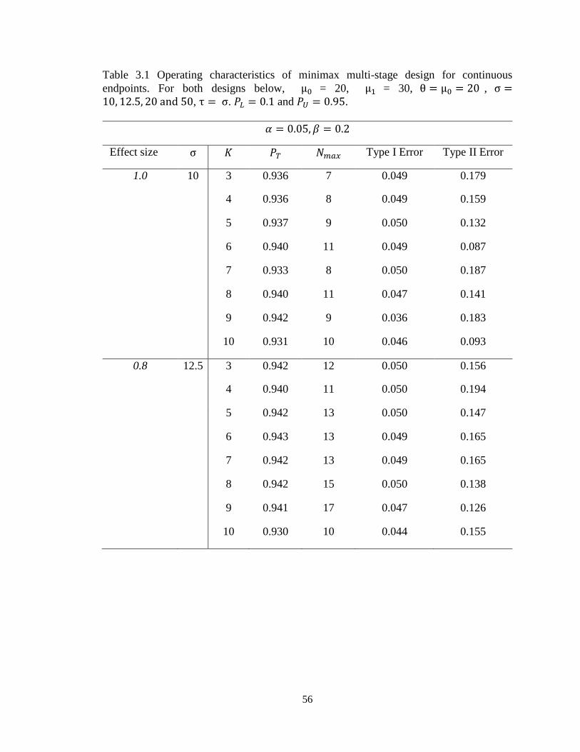
56

Table 3.1 Operating characteristics of minimax multi-stage design for continuous

endpoints. For both designs below, μ0 = 20, μ1 = 30, θ = μ0 = 20 , σ =10, 12.5, 20 and 50, τ = σ. 𝑃𝐿 = 0.1 and 𝑃𝑈 = 0.95.

𝛼 = 0.05, 𝛽 = 0.2

Effect size σ 𝐾 𝑃𝑇 𝑁𝑚𝑎𝑥 Type I Error Type II Error

1.0 10 3 0.936 7 0.049 0.179

4 0.936 8 0.049 0.159

5 0.937 9 0.050 0.132

6 0.940 11 0.049 0.087

7 0.933 8 0.050 0.187

8 0.940 11 0.047 0.141

9 0.942 9 0.036 0.183

10 0.931 10 0.046 0.093

0.8 12.5 3 0.942 12 0.050 0.156

4 0.940 11 0.050 0.194

5 0.942 13 0.050 0.147

6 0.943 13 0.049 0.165

7 0.942 13 0.049 0.165

8 0.942 15 0.050 0.138

9 0.941 17 0.047 0.126

10 0.930 10 0.044 0.155

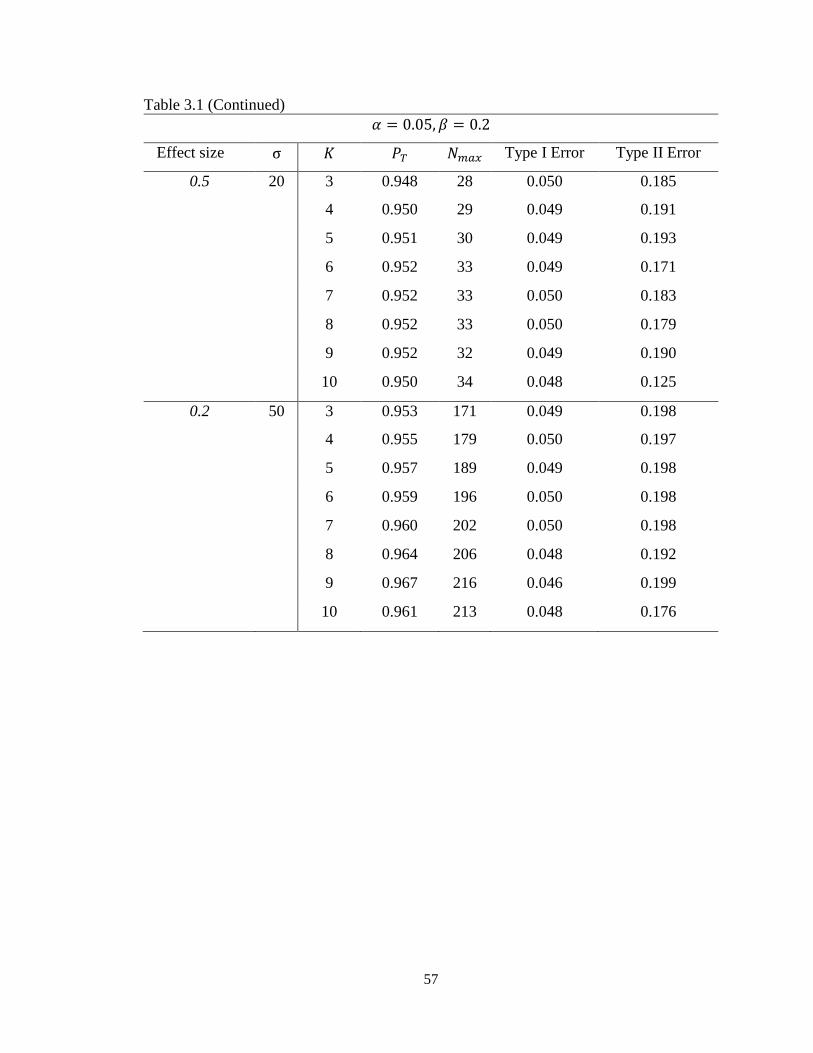
57

Table 3.1 (Continued)

𝛼 = 0.05, 𝛽 = 0.2

Effect size σ 𝐾 𝑃𝑇 𝑁𝑚𝑎𝑥 Type I Error Type II Error

0.5 20 3 0.948 28 0.050 0.185

4 0.950 29 0.049 0.191

5 0.951 30 0.049 0.193

6 0.952 33 0.049 0.171

7 0.952 33 0.050 0.183

8 0.952 33 0.050 0.179

9 0.952 32 0.049 0.190

10 0.950 34 0.048 0.125

0.2 50 3 0.953 171 0.049 0.198

4 0.955 179 0.050 0.197

5 0.957 189 0.049 0.198

6 0.959 196 0.050 0.198

7 0.960 202 0.050 0.198

8 0.964 206 0.048 0.192

9 0.967 216 0.046 0.199

10 0.961 213 0.048 0.176

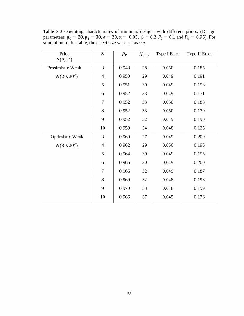
58

Table 3.2 Operating characteristics of minimax designs with different priors. (Design

parameters: μ0 = 20, μ1 = 30, σ = 20, α = 0.05, β = 0.2, 𝑃𝐿 = 0.1 and 𝑃𝑈 = 0.95). For

simulation in this table, the effect size were set as 0.5.

Prior

N(𝜃, 𝜏2)

K 𝑃𝑇 𝑁𝑚𝑎𝑥 Type I Error Type II Error

Pessimistic Weak 3 0.948 28 0.050 0.185

𝑁(20, 202) 4 0.950 29 0.049 0.191

5 0.951 30 0.049 0.193

6 0.952 33 0.049 0.171

7 0.952 33 0.050 0.183

8 0.952 33 0.050 0.179

9 0.952 32 0.049 0.190

10 0.950 34 0.048 0.125

Optimistic Weak 3 0.960 27 0.049 0.200

𝑁(30, 202) 4 0.962 29 0.050 0.196

5 0.964 30 0.049 0.195

6 0.966 30 0.049 0.200

7 0.966 32 0.049 0.187

8 0.969 32 0.048 0.198

9 0.970 33 0.048 0.199

10 0.966 37 0.045 0.176

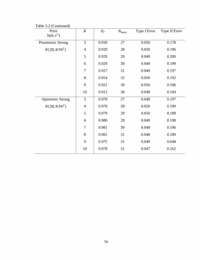
59

Table 3.2 (Continued)

Prior

N(𝜃, 𝜏2)

K 𝑃𝑇 𝑁𝑚𝑎𝑥 Type I Error Type II Error

Pessimistic Strong 3 0.930 27 0.050 0.178

𝑁(20, 8.942) 4 0.929 28 0.050 0.196

5 0.929 29 0.049 0.200

6 0.929 30 0.049 0.199

7 0.927 31 0.049 0.197

8 0.924 32 0.050 0.192

9 0.921 30 0.050 0.186

10 0.912 30 0.048 0.104

Optimistic Strong 3 0.978 27 0.048 0.197

𝑁(30, 8.942) 4 0.978 28 0.050 0.190

5 0.979 29 0.050 0.189

6 0.980 29 0.049 0.198

7 0.981 30 0.048 0.196

8 0.981 31 0.048 0.189

9 0.975 31 0.049 0.048

10 0.978 31 0.047 0.162

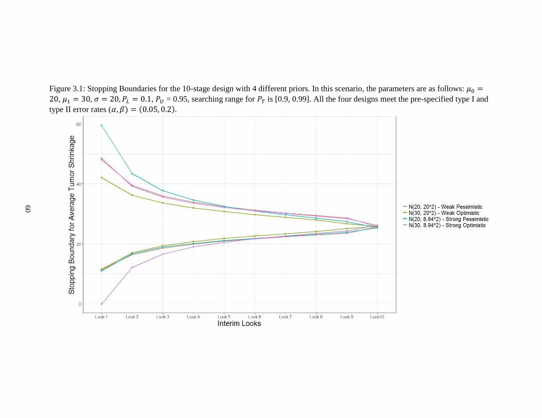
60

Figure 3.1: Stopping Boundaries for the 10-stage design with 4 different priors. In this scenario, the parameters are as follows: 𝜇0 =

20, 𝜇1 = 30, 𝜎 = 20, 𝑃𝐿 = 0.1, 𝑃𝑈 = 0.95, searching range for 𝑃𝑇 is [0.9, 0.99]. All the four designs meet the pre-specified type I and

type II error rates (𝛼, 𝛽) = (0.05, 0.2).

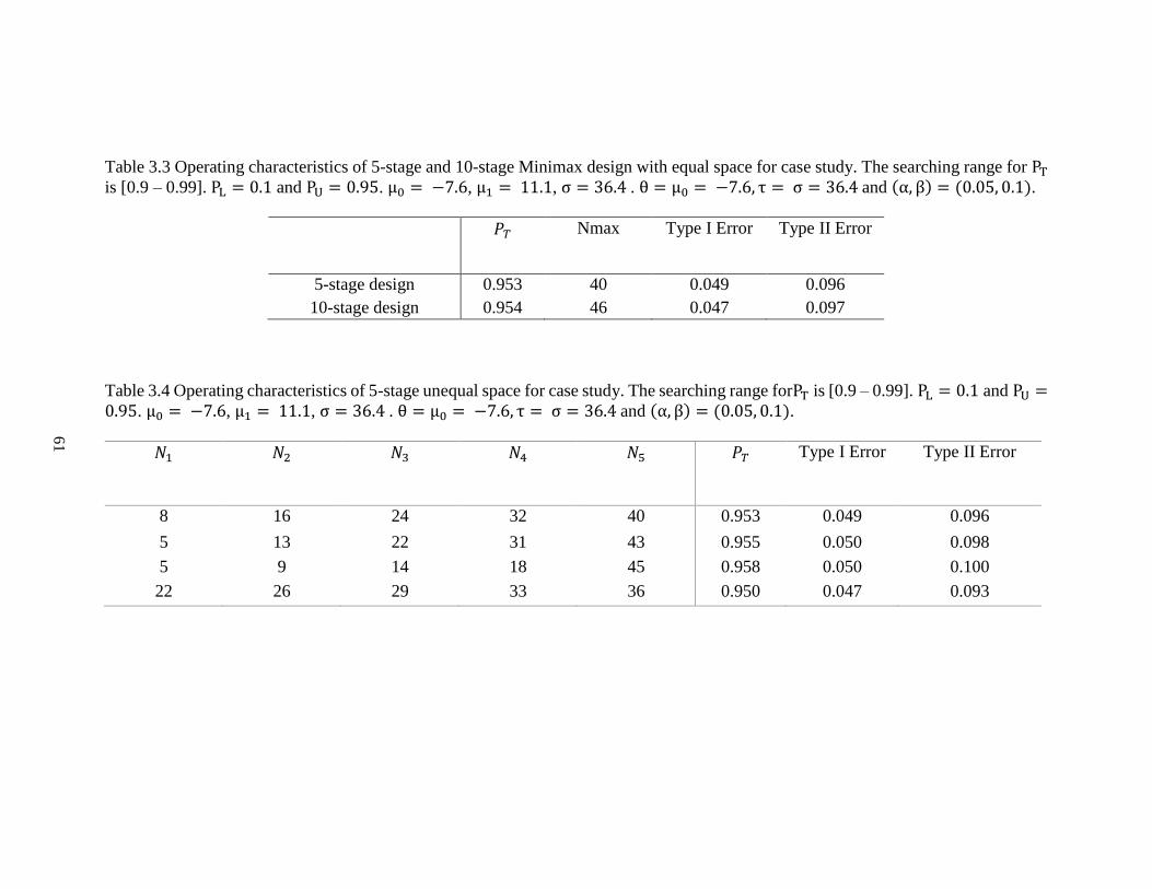
61

Table 3.3 Operating characteristics of 5-stage and 10-stage Minimax design with equal space for case study. The searching range for PT

is [0.9 – 0.99]. PL = 0.1 and PU = 0.95. μ0 = −7.6, μ1 = 11.1, σ = 36.4 . θ = μ0 = −7.6, τ = σ = 36.4 and (α, β) = (0.05, 0.1).

𝑃𝑇 Nmax Type I Error Type II Error

5-stage design 0.953 40 0.049 0.096

10-stage design 0.954 46 0.047 0.097

Table 3.4 Operating characteristics of 5-stage unequal space for case study. The searching range forPT is [0.9 – 0.99]. PL = 0.1 and PU =0.95. μ0 = −7.6, μ1 = 11.1, σ = 36.4 . θ = μ0 = −7.6, τ = σ = 36.4 and (α, β) = (0.05, 0.1).

𝑁1 𝑁2 𝑁3 𝑁4 𝑁5 𝑃𝑇 Type I Error Type II Error

8 16 24 32 40 0.953 0.049 0.096

5 13 22 31 43 0.955 0.050 0.098

5 9 14 18 45 0.958 0.050 0.100

22 26 29 33 36 0.950 0.047 0.093

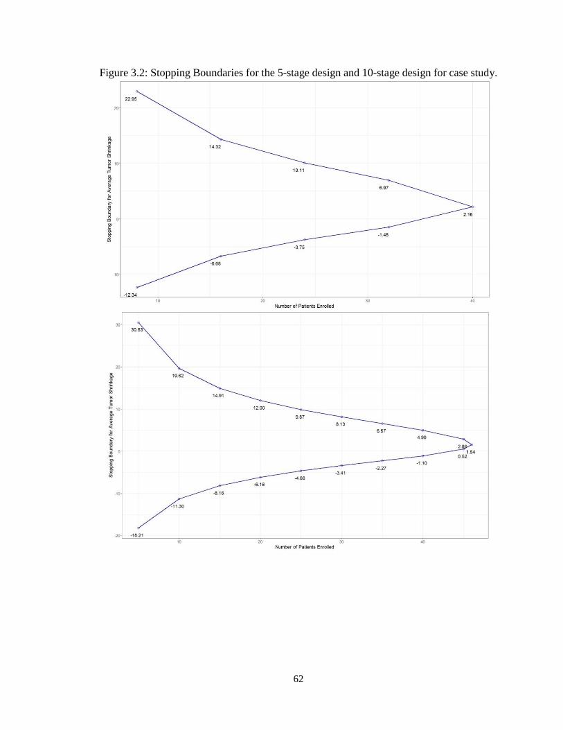
62

Figure 3.2: Stopping Boundaries for the 5-stage design and 10-stage design for case study.

63

CHAPTER FOUR

PPSC: An R Package for Single-Arm Phase II Predictive Probability Design with

Continuous Endpoints

4.1 Abstract

In practice, interim analyses are usually incorporated into a trial to stop the trial

early either due to futility and/or superiority. Early stopping of the trial can prevent patient

exposure to ineffective therapies or accelerate drug development if beneficial effects are

observed. In the Bayesian framework, interim designs based on predictive probability

provide a flexible way to monitor the trial continuously while incorporating the evidence

from the current data and making inference for the future. We extended a predictive

probability design for binary outcomes into a single-arm trial setting for continuous

outcomes and provide both optimal and minimax designs. In this paper, we describe the

usage and implementation of the R package PPSC, which aims to implement a grid search

strategy to find the optimal and minimax designs for continuous outcomes based on

predictive probability. The package PPSC contains two functions and provides the

solutions for both two-stage and multi-stage designs. These two functions give clinical

investigators and biostatisticians the flexibility to monitor the trial and provide the stopping

boundaries for futility and efficacy when early stopping the trial is desired.

Keywords: predictive probability; continuous outcome; interim design; phase II; R.

4.2 Introduction

A conventional phase II trial aims to evaluate the treatment effect of a drug or

therapy being studied and identify the promising ones to carry on to the confirmative phase

III trials. Interim strategies are of great importance in each stage of clinical trials. As

64

developed for protecting participants from unsafe drugs or to hasten the general

implementation of a beneficial therapy, interim strategies can be utilized to stop the trials

early either for safety, futility or efficacy [14].

Many statistical methods have been developed for phase II trial designs, for both

two-stage and multi-stage designs, regarding different types of endpoints. For binary

endpoints, Gehan developed a two-stage design to stop the trial early due to futility if no

response is observed from the first stage [18]. Simon proposed both optimal design and

minimax design allowing one interim stop for futility [19]. Several extensions of Simon’s

design have been proposed [20, 21, 78]. Recent years, Bayesian approaches have been

widely applied in the clinical trial designs. In particular, Tan and Machin proposed a two-

stage design based on posterior distribution of the true response rate and Sambucini

extended it into predictive version [29-31]. Dong et al. suggested a two-stage design

incorporating both frequentist and Bayesian error rates [39].

Regarding multi-stage designs, group-sequential designs are widely used in

practice, in which groups of patients, either equally spaced or unequally spaced, are

enrolled and the hypothesis is tested multiple times during accrual the trial. The most

popular group sequential designs are O’Brian-Fleming’ design and Pocock’s design [62,

63]. Jennison ad Turnbull provide an thorough overview of group-sequential methodology

[74]. Under Bayesian framework, in particular, Lee and Liu developed a predictive

probability design for the binary response rate to continuously monitor the trial [37].

We extended Lee and Liu’s predictive probability design into a setting for

continuous outcome. This paper introduces an R package, PPSC, which provides the

implementation of our extended predictive probability designs. This package specifically

65

incorporates two types of designs: the two-stage design and the multi-stage design. The

two-stage design is primarily for the purpose of early stopping due to futility, while it also

has the capacity to stop early due to efficacy. The multi-stage design allows early stopping

of the trial due to either futility or efficacy, which can accommodate up to 40 stages with

39 interim looks.

The paper is organized as follows. Section 4.3 describes the both two-stage design

and multi-stage design as well as the trial decision rules. Section 4.4 details the

implementation of the two main functions in the package and gives a series of examples of

how to use the options in the functions. Section 4.5 discusses the limitations and future

directions for current design and package.

4.3 Methods

For both two-stage and multi-stage designs, the hypothesis testing framework is as

follows:

𝐻0: 𝜇 ≤ 𝜇0 vs. 𝐻1: 𝜇 ≥ 𝜇1

where 𝜇0 represents the maximum efficacy from the standard treatment or historical

control, while 𝜇1 represents a target efficacy threshold from the treatment or therapy being

investigated. Both designs meet pre-specified Type I and Type II error rate constraints.

For illustration purposes, we use tumor shrinkage as an example of continuous

outcomes. However, this design is not limited to tumor shrinkage. It could be used for

changes in biomarkers, pre-post designs or any other continuous endpoints. We present

this one example throughout for simplicity. Here, we define “tumor size change/tumor

shrinkage” as the percentage decrease in the sum of the longest diameter of the target

66

lesions compared to baseline for each patient, with positive values denoting tumor

shrinkage. We assume the average tumor shrinkage, 𝑋 , follows a normal distribution

𝑁( 𝜇, 𝜎2), with mean 𝜇 and known variance 𝜎2. We assume a normal conjugate prior

distribution for 𝜇, 𝑁(𝜃, 𝜏2) and we use effective sample size for the prior (ESS), the ratio

of likelihood variance to prior variance ( 𝜎2

𝜏2) for the normal case, to assign the amount of

information for the prior [67]. For the purpose of simulation, we set ESS = 1, assuming

very little knowledge is known before the trial starts. In practice, ESS and priors should be

input from the investigators and represent the investigator’s previous knowledge of the

tumor size change or endpoint being studied from standard treatment or historical control.

We generalized the notation for the two-stage design to be a special case of the

multi-stage design. We consider a single-arm trial with a total sample size of 𝑁𝑚𝑎𝑥 and

total 𝐾 stages, where 𝐾 ≤ 𝑁𝑚𝑎𝑥. When K = 2, it represents the two-stage design. At the

end of 𝑖𝑡ℎ stage, the number of patients enrolled in total is denoted as 𝑛𝑖 , where 𝑖 =

1, 2, … , 𝐾. We denote the average tumor shrinkage for 𝑛𝑖 patients as �̅�𝑛𝑖. Therefore, given

the information from these current 𝑛𝑖 patients, the posterior distribution of the mean tumor

shrinkage 𝜇 follows a normal distribution, with mean 𝜎2𝜃

𝑛𝑖𝜏2+𝜎2

+ 𝑛𝑖𝜏

2

𝑛𝑖𝜏2+𝜎2

�̅�𝑛𝑖 and variance

𝜏2𝜎2

𝑛𝑖𝜏2+𝜎2

. Thus, the average tumor shrinkage from the future 𝑚𝑖 patients, where 𝑚𝑖 =

𝑁𝑚𝑎𝑥 − 𝑛𝑖, follows a normal distribution with mean 𝜇𝑝∗ and 𝜎𝑝

∗2, where

𝜇𝑝∗ =

𝜎2𝜃

(𝑚𝑖 + 𝑛𝑖)𝜏2 + 𝜎2+

𝑛𝑖𝜏2

(𝑚𝑖 + 𝑛𝑖)𝜏2 + 𝜎2�̅�𝑛𝑖 +

𝑚𝑖𝜏2�̅�𝑚𝑖

(𝑚𝑖 + 𝑛𝑖)𝜏2 + 𝜎2

𝜎𝑝∗2 =

𝜏2𝜎2

(𝑚𝑖 + 𝑛𝑖)𝜏2 + 𝜎2

67

We define 𝐵𝑖 = 𝑃𝑟𝑜𝑏(𝜇∗ > 𝜇0|�̅�𝑛𝑖 , �̅�𝑚𝑖) to measure the probability that the mean tumor

shrinkage is larger than 𝜇0, given the mean tumor size change in current 𝑛𝑖 patients and

future 𝑚𝑖 patients. We can conclude the treatment is efficacious when 𝐵𝑖 > 𝑃𝑇, where 𝑃𝑇

is the posterior critical value at each stage and is usually assumed to be greater than 0.8.

𝐵𝑖 = 𝑃𝑟𝑜𝑏(𝜇∗ > 𝜇0|�̅�𝑛𝑖 , �̅�𝑚𝑖) = 1 − 𝑃𝑟𝑜𝑏(𝜇∗ ≤ 𝜇0|�̅�𝑛𝑖 , �̅�𝑚𝑖)

= 1 − 𝛷 (𝜇0− 𝜇𝑝

∗

𝜎𝑝∗ ) > 𝑃𝑇

where 𝛷 ( ∙) represents the cumulative density function (CDF) of the standard normal

distribution. The above inequality (1) can be derived into an inequality of �̅�𝑚𝑖 regarding

𝜃𝑇.

�̅�𝑚𝑖 >((𝑛𝑖+𝑚𝑖)𝜏

2+𝜎2)(𝜇0− 𝜎𝑝∗𝛷−1(1−𝑃𝑇))− 𝜎

2𝜃−𝜏2𝑛𝑖�̅�𝑛𝑖

𝑚𝑖𝜏2 = 𝛿

The posterior predictive distribution of tumor size change from the future 𝑚 patients also

follows a normal distribution 𝑁(𝜇𝑝, 𝜎𝑝2) , with 𝜇𝑝 =

𝜎2𝜃

𝑛𝑖𝜏2+𝜎2

+ 𝑛𝑖𝜏

2

𝑛𝑖𝜏2+𝜎2

�̅�𝑛𝑖 and 𝜎𝑝2 =

𝜎2

𝑚𝑖+

𝜏2𝜎2

𝑛𝑖𝜏2+𝜎2

.

Based on all the information above, we can then define the predictive probability (𝑃𝑃)

Predictive probability (𝑃𝑃) = 𝑃𝑟𝑜𝑏(�̅�𝑚𝑖 > 𝛿|�̅�𝑛𝑖)

= 1 − 𝑃𝑟𝑜𝑏(�̅�𝑚𝑖 ≤ 𝛿|�̅�𝑛𝑖) = 1 − 𝛷 (𝛿 − 𝜇𝑝

𝜎𝑝)

(1)

(2)

(3)

68

A high 𝑃𝑃 means that given current data, the treatment is likely to be efficacious by the

end of the study; whereas a low 𝑃𝑃 suggests that the treatment may not have sufficient

activity. Therefore, we use 𝑃𝑃 to make the decision during the interims in the trial.

If 𝑃𝑃𝑖 < 𝑃𝐿, stop the trial and reject the alternative hypothesis;

If 𝑃𝑃𝑖 > 𝑃𝑈, stop the trial and reject the null hypothesis;

Otherwise, continue to the next stage.

𝑃𝑃𝑖 can also be transformed into �̅�𝑛𝑖, and the trial decision rules can be made according

to the futility and efficacy boundaries at the end of each stage.

Although our design stopping boundaries are based on Bayesian predictive

probabilities, we additionally restrict our designs to satisfy pre-specified type I and type II

error rates constraints. Therefore, we need to calculate the probability of rejecting the null

hypothesis at each stage. The detailed calculations for type I error rates and power are

documented in Chapter 2 and 3.

4.4 Use of the package PPSC

Package PPSC depends on three libraries: R2Cuba, cubature and ggplot2 [76, 77,

79]. Packages cubature and R2Cuba are employed to conduct the multidimensional

integration either using direct numeric integration or Monte Carlo algorithm. When the

design has more than three stages, integration using Monte Carlo algorithm is much faster

than numeric integration. Package ggplot2 is utilized to plot the design stopping boundaries.

Both designs give clinical investigators and biostatisticians the flexibility to monitor the

trial and stop the trial early when necessary.

69

Package PPSC contains two functions, par2stage and parmultistage. Function

par2stage conducts a single-arm PP design, which incorporates one interim look, allowing

for early stopping only due to futility. Function parmultestage performs a single-arm PP

design allows for early stopping due to both futility and superiority, and currently allows

for up to 40 interim looks. Regardless of design selected, input options are described in

Table 4.1 and Table 4.2.

For both functions, there are several arguments in common. To implement the two

designs, the users should specify a couple of parameters: the likelihood standard deviation

“sigma” (𝜎); the mean “theta” (𝜃) and standard deviation “tau” (𝜏) for the normal conjugate

priors, which represents the previous knowledge about the endpoint from the investigators;

the null value “mu0” (𝜇0) and alternative value “mu1” (𝜇1) for the hypothesis testing; the

low and high boundaries for the posterior probability (𝑃𝑇) , “pTlow” and ”pThigh”, as well

as the searching increment for (𝑃𝑇), “pTby”. As defined in Lee and Liu’s design, 𝑃𝑇 is

usually a large number between [0.8, 1], while Dong et al. suggest a larger number such as

0.95 [37, 39]. The default setting is “pTlow = 0.9, pThigh = 0.99 and pTby = 0.01”. For

the two-stage design, users also need to specify the low and high boundaries for the

predictive probability (𝑃𝐿), “pLlow” and ”pLhigh”, as well as the searching increment for

(𝑃𝐿), “pLby”. 𝑃𝐿 is usually a small number below 0.1. The default setting is “pLlow = 0.01,

pLhigh = 0.1 and pLby = 0.01”. Although two-stage design is primarily for early

termination due to futility, the trial can also stop early for efficacy. To do so, the user can

specify the upper boundary for the predictive probability (𝑃𝑈), “pU”, which is usually a

large number greater than 0.9. The default value is 0.95. In addition, for the multi-stage

design, users have the flexibility of specifying the following parameters: if the trial is

70

continuously monitored “continuous”, with the default value “F”; the number of interims

looks involved in the trial “num.interim”, with the default value “num.interim = 2” for the

3-stage design; if the number of patients at each stage is the same “equal.space”, with

default setting “equal.space = T” for the same number of patients at each stage. Further,

for both designs, the users need to specify the type I and type II error rates constraints,

“pre.typeIerror” and “pre.typeIIerror”. The default settings are “pre.typeIerror = 0.05” and

“pre.typeIIerror = 0.2”. The plot for stopping boundaries can be outputted with the

argument “plot_yes” being “T”.

Another argument for both function is “plot_yes”, for which if the value is “T”, the

plot for stopping boundaries is outputted.

4.4.1 Two-stage design for early stopping due to futility: use of par2stage

Example 1:

Consider the situation where the standard therapy or historical control will lead the

tumor shrinkage up to 20% shrinkage and the clinical investigators want to test if the new

therapy will improve the tumor shrinkage to at least 30%. The trial only allows for early

stopping due to futility. Therefore, we set pU = 1. The likelihood standard deviation in this

example is assumed to be 20, which should be input from the investigator or from historical

control data. If we assume little information is known before the trials starts, we use ESS

= 1. Thus, theta = 20 and tau = 20. The searching range for pL is to be [0.01, 0.1] and for

pT is to be [0.9, 0.99]. The increment for grid search is 0.01 for both pT and pL. The pre-

specified type I error rate is set to 0.05, and type II error rate is set to 0.2. The R code

necessary to run this scenario is:

71

Example1 <- par2stage (sigma = 20, tau = 20, theta = 20, mu0 = 20, mu1 = 30,

pTlow = 0.90, pThigh = 0.99, pTby = 0.01, pLlow = 0.01, pLhigh = 0.1, pLby = 0.01, pU

= 1, pre.typeIerror = 0.05, pre.typeIIerror = 0.2, plot_yes = T)

The output is a list containing two elements, which give the operating

characteristics for both optimal design and minimax design. In terms of the optimal design,

the total sample size required is 27 with 11 for the first stage. The futility boundaries for

first and second stage are 20.681 and 26.447. The corresponding type I and type II error

rates are 0.044 and 0.199. The pT and pL that yield the optimal design are 0.95 and 0.1.

The minimax design yields a very similar parameter combination, with 26 as the total

sample size, 14 as the sample size for the first stage, 21.048 and 26.575 as the futility

boundaries.

$`Optimal Design`

[1]

Total Sample Size 27

Sample Size for the First Stage 11

Futility Boundaries at the End of the First Stage 20.681

Futility Boundaries at the End of the Second Stage 26.447

Probability of Early Termination 0.545

Expected Sample Size under the null 18.281

Type I Error 0.044

Type II Error 0.199

pT 0.950

pL 0.100

[2]

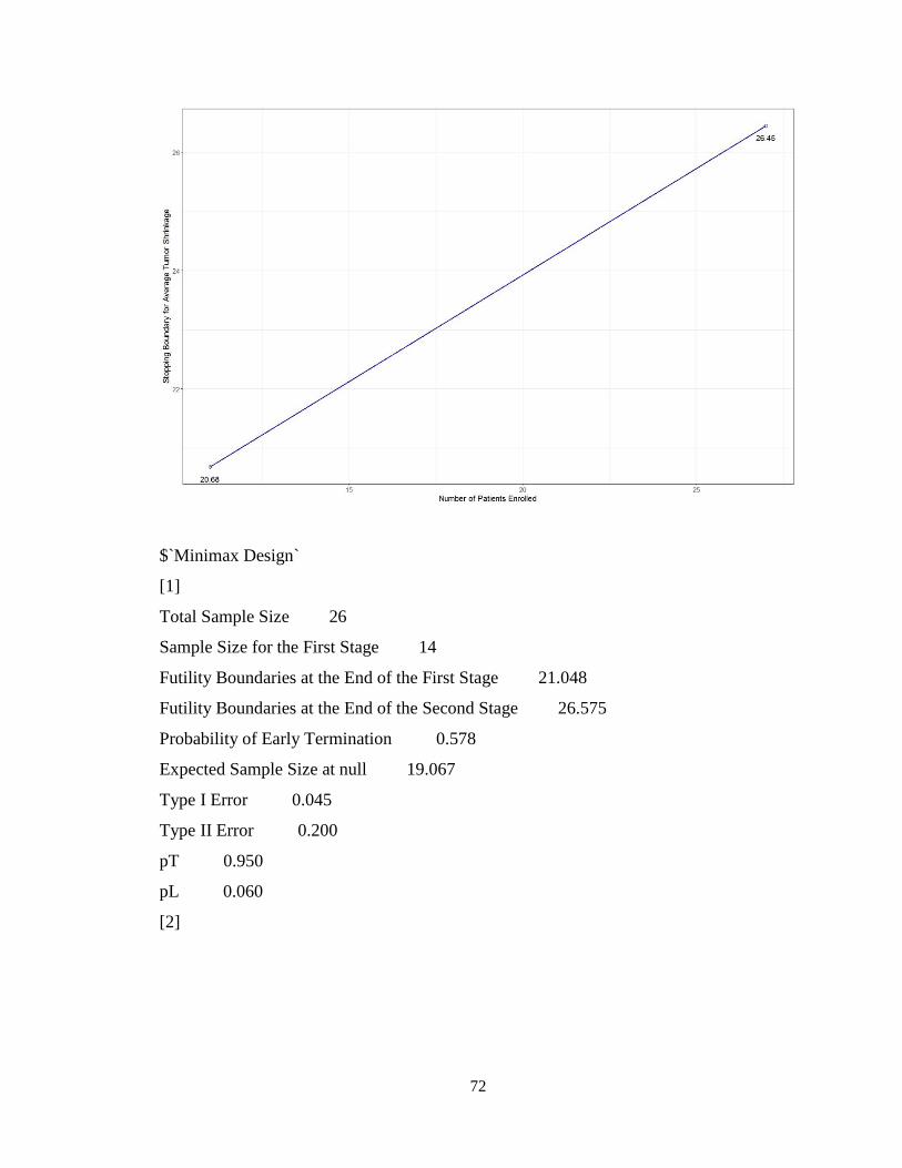
72

$`Minimax Design`

[1]

Total Sample Size 26

Sample Size for the First Stage 14

Futility Boundaries at the End of the First Stage 21.048

Futility Boundaries at the End of the Second Stage 26.575

Probability of Early Termination 0.578

Expected Sample Size at null 19.067

Type I Error 0.045

Type II Error 0.200

pT 0.950

pL 0.060

[2]

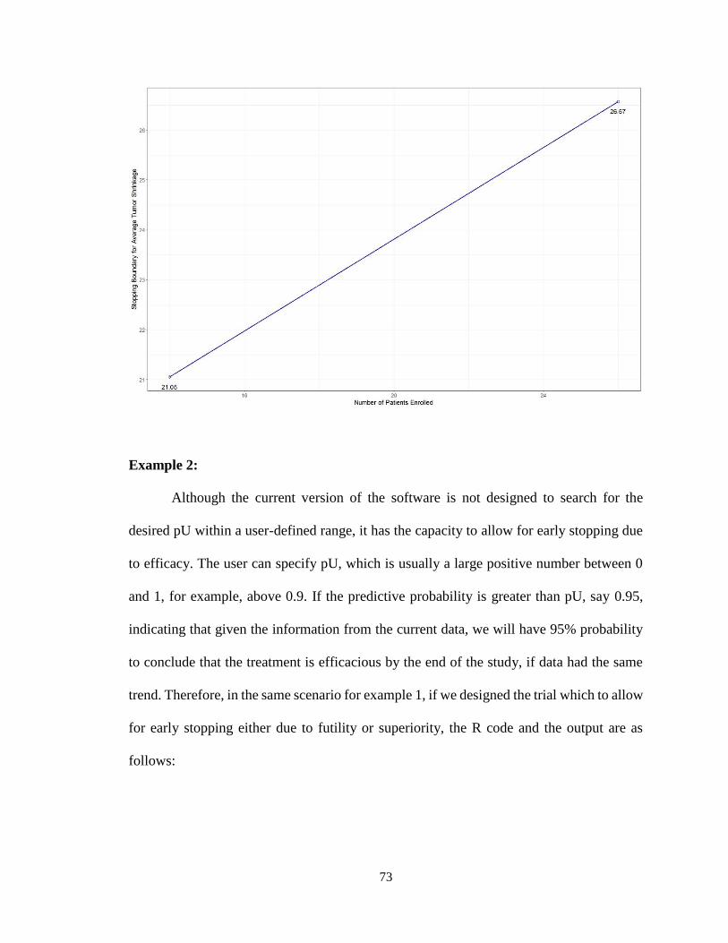
73

Example 2:

Although the current version of the software is not designed to search for the

desired pU within a user-defined range, it has the capacity to allow for early stopping due

to efficacy. The user can specify pU, which is usually a large positive number between 0

and 1, for example, above 0.9. If the predictive probability is greater than pU, say 0.95,

indicating that given the information from the current data, we will have 95% probability

to conclude that the treatment is efficacious by the end of the study, if data had the same

trend. Therefore, in the same scenario for example 1, if we designed the trial which to allow

for early stopping either due to futility or superiority, the R code and the output are as

follows:

74

Example2 <- par2stage (sigma = 20, tau = 20, theta = 20, mu0 = 20, mu1 = 30,

pTlow = 0.9, pThigh = 0.99, pTby = 0.01, pLlow = 0.01, pLhigh = 0.1, pLby = 0.01, pU =

0.95, pre.typeIerror = 0.05, pre.typeIIerror = 0.2, plot_yes = T)

$`Optimal Design`

[1]

Total Sample Size 27

Sample Size for the First Stage 10

Futility Boundaries at the End of the First Stage 20.215

Futility Boundaries at the End of the Second Stage 26.447

Efficacy Boundaries at the end of the First Stage 35.340

Efficacy Boundaries at the End of the Second Stage 26.447

Probability of Early Termination 0.521

Expected Sample Size at null 18.140

Type I Error 0.048

Type II Error 0.197

pT 0.950

pL 0.100

[2]

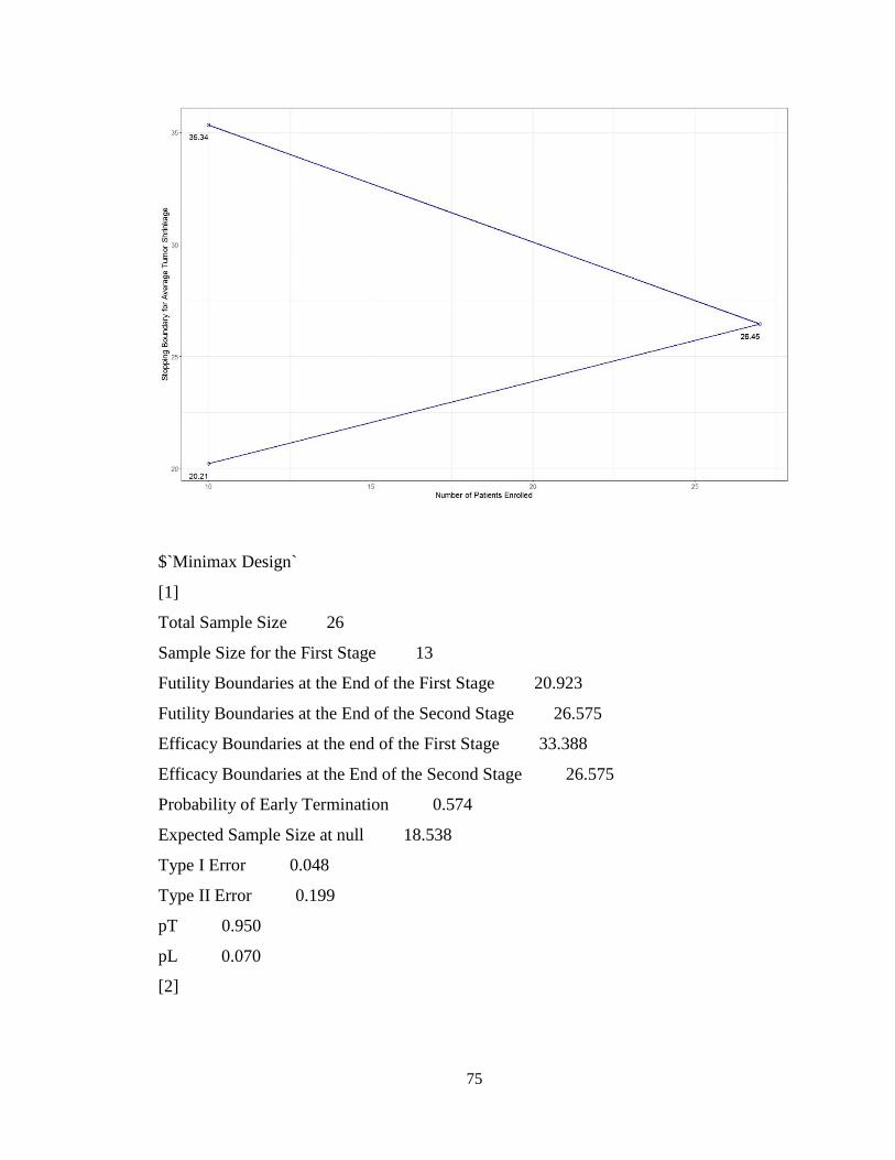
75

$`Minimax Design`

[1]

Total Sample Size 26

Sample Size for the First Stage 13

Futility Boundaries at the End of the First Stage 20.923

Futility Boundaries at the End of the Second Stage 26.575

Efficacy Boundaries at the end of the First Stage 33.388

Efficacy Boundaries at the End of the Second Stage 26.575

Probability of Early Termination 0.574

Expected Sample Size at null 18.538

Type I Error 0.048

Type II Error 0.199

pT 0.950

pL 0.070

[2]

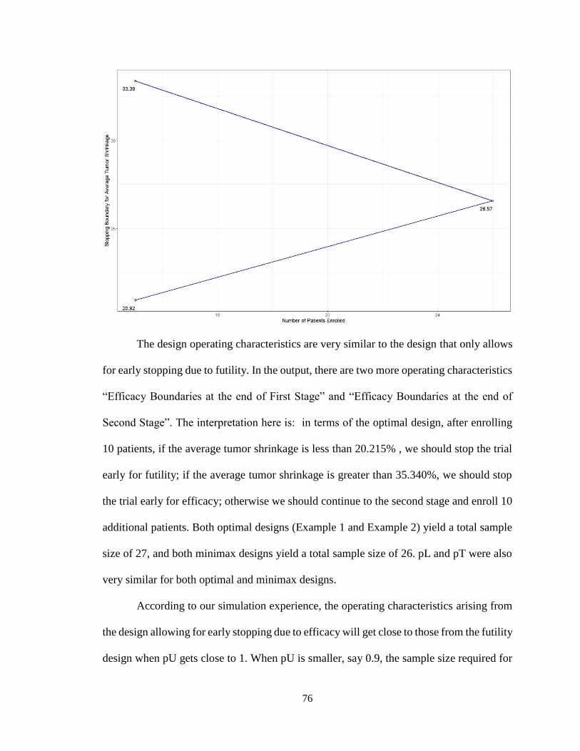
76

The design operating characteristics are very similar to the design that only allows

for early stopping due to futility. In the output, there are two more operating characteristics

“Efficacy Boundaries at the end of First Stage” and “Efficacy Boundaries at the end of

Second Stage”. The interpretation here is: in terms of the optimal design, after enrolling

10 patients, if the average tumor shrinkage is less than 20.215% , we should stop the trial

early for futility; if the average tumor shrinkage is greater than 35.340%, we should stop

the trial early for efficacy; otherwise we should continue to the second stage and enroll 10

additional patients. Both optimal designs (Example 1 and Example 2) yield a total sample

size of 27, and both minimax designs yield a total sample size of 26. pL and pT were also

very similar for both optimal and minimax designs.

According to our simulation experience, the operating characteristics arising from

the design allowing for early stopping due to efficacy will get close to those from the futility

design when pU gets close to 1. When pU is smaller, say 0.9, the sample size required for

77

the first stage will be larger. The probability of early termination also increases. The total

sample size will be 26 with the probability of early termination 0.722.

Example 1 and 2 explain the usage of function par2stage to perform the two-stage

design. Both optimal design and minimax design are included in the output. The stopping

boundaries are also displayed if the value for “plot_yes” argument is “T”.

4.4.2 Multi-stage design for early stopping due to both futility and efficacy: use of

parmultistage

Example 3:

Consider the same scenario from the previous examples in the two-stage design

setting. The investigators want to incorporate more than one interim look during the entire

trial. The standard therapy or historical control will lead to tumor shrinkage up to 20%, and

the clinical investigators want to test if the new therapy will improve the tumor shrinkage

up to at least 30%. All the other parameters are assumed to be the same.

In current version, for the multistage design, we are only allowed to search the

range for pT, but not for pL and pU, due to intensive computation time. The user should

pre-specify a single value for pL and pU, for example, pL = 0.1 and pU = 0.95. Usually, as

mentioned above, pL is a small number and pU is a large number between 0 and 1. The

pre-specified type I error rate and type II error rate were still set to be 0.05 and 0.2. In

addition, this current version can only display the minimax design also due to the

computing time and searching strategy. If the investigators want to incorporate 3 interim

looks during the entire trial with sample size equally spaced and the searching range for pT

is still set as [0.9, 0.99], the R-code to execute is as follows:

Example3 <- parmultistage(continuous = F, first.look = NULL, num.interim = 3 ,

equal.spaced = T , user.p = NULL , sigma = 20, tau = 20, mu0 = 20, mu1 = 30 , theta = 20,

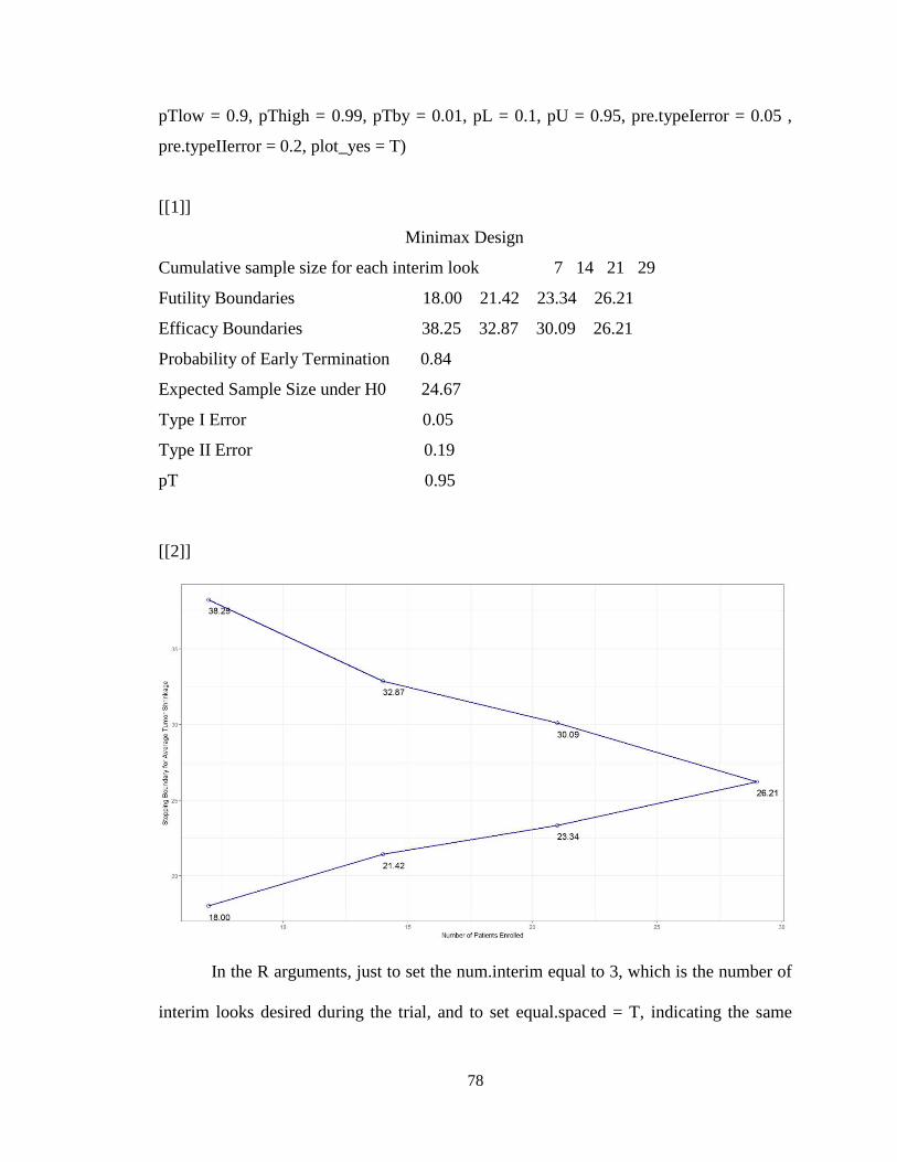
78

pTlow = 0.9, pThigh = 0.99, pTby = 0.01, pL = 0.1, pU = 0.95, pre.typeIerror = 0.05 ,

pre.typeIIerror = 0.2, plot_yes = T)

[[1]]

Minimax Design

Cumulative sample size for each interim look 7 14 21 29

Futility Boundaries 18.00 21.42 23.34 26.21

Efficacy Boundaries 38.25 32.87 30.09 26.21

Probability of Early Termination 0.84

Expected Sample Size under H0 24.67

Type I Error 0.05

Type II Error 0.19

pT 0.95

[[2]]

In the R arguments, just to set the num.interim equal to 3, which is the number of

interim looks desired during the trial, and to set equal.spaced = T, indicating the same

79

number of patients at each stage is desired. Sometimes, when we set the interim looks

equally spaced through the trial, sample size in the last stage may deviate slightly from

previous stages. In this example, the sample size for the last stage is 8, instead of 7 as the

first three stages. This discrepancy is due to rounding errors. If we set plot_yes = T, the

output from parmultistage function is a list containing two elements. The first element is

the operating characteristics for the minimax design resulting from the user-specified

parameters, including the sample size and futility/ efficacy boundaries for each interim

look, probability of termination, expected sample size under the null hypothesis and type

I/II error rates. The second element is a plot for stopping boundaries, with y-axis being the

upper and lower boundaries for trial stopping rules, and x-axis being the cumulative

number of patients at each interim look. To hide the plot, set plot_yes equal to F.

Example 4:

If the investigators prefer not to space looks at the data equally, they can also define

the cumulative proportion of the sample size regarding each interim look. For example,

instead of equally spaced interim looks, the investigators can set user.p = c(0.1, 0.4, 0.8,

1.0) and equal.spaced = F, if they want to analyze the data from the trial after 10%, 40% ,

80% and 100% of the patients are enrolled. They can stop the trial at each of the interim

looks either due to futility or efficacy. The R code is as follows:

Example4 <- parmultistage(continuous = F, first.look = NULL, num.interim = 3 ,

equal.spaced = F, user.p = c(0.1, 0.4, 0.8, 1.0), sigma = 20, tau = 20, mu0 = 20, mu1 = 30 ,

theta = 20, pTlow = 0.9, pThigh = 0.99, pTby = 0.01, pL = 0.1, pU = 0.95, pre.typeIerror

= 0.05 , pre.typeIIerror = 0.2, plot_yes = T)

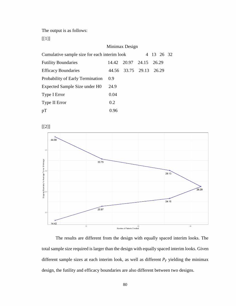
80

The output is as follows:

[[1]]

Minimax Design

Cumulative sample size for each interim look 4 13 26 32

Futility Boundaries 14.42 20.97 24.15 26.29

Efficacy Boundaries 44.56 33.75 29.13 26.29

Probability of Early Termination 0.9

Expected Sample Size under H0 24.9

Type I Error 0.04

Type II Error 0.2

pT 0.96

[[2]]

The results are different from the design with equally spaced interim looks. The

total sample size required is larger than the design with equally spaced interim looks. Given

different sample sizes at each interim look, as well as different 𝑃𝑇 yielding the minimax

design, the futility and efficacy boundaries are also different between two designs.

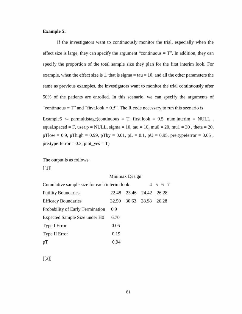
81

Example 5:

If the investigators want to continuously monitor the trial, especially when the

effect size is large, they can specify the argument “continuous = T”. In addition, they can

specify the proportion of the total sample size they plan for the first interim look. For

example, when the effect size is 1, that is sigma = tau = 10, and all the other parameters the

same as previous examples, the investigators want to monitor the trial continuously after

50% of the patients are enrolled. In this scenario, we can specify the arguments of

“continuous = T” and “first.look = 0.5”. The R code necessary to run this scenario is

Example5 <- parmultistage(continuous = T, first.look = 0.5, num.interim = NULL ,

equal.spaced = F, user.p = NULL, sigma = 10, tau = 10, mu0 = 20, mu1 = 30 , theta = 20,

pTlow = 0.9, pThigh = 0.99, pTby = 0.01, pL = 0.1, pU = 0.95, pre.typeIerror = 0.05 ,

pre.typeIIerror = 0.2, plot_yes = T)

The output is as follows:

[[1]]

Minimax Design

Cumulative sample size for each interim look 4 5 6 7

Futility Boundaries 22.48 23.46 24.42 26.28

Efficacy Boundaries 32.50 30.63 28.98 26.28

Probability of Early Termination 0.9

Expected Sample Size under H0 6.70

Type I Error 0.05

Type II Error 0.19

pT 0.94

[[2]]

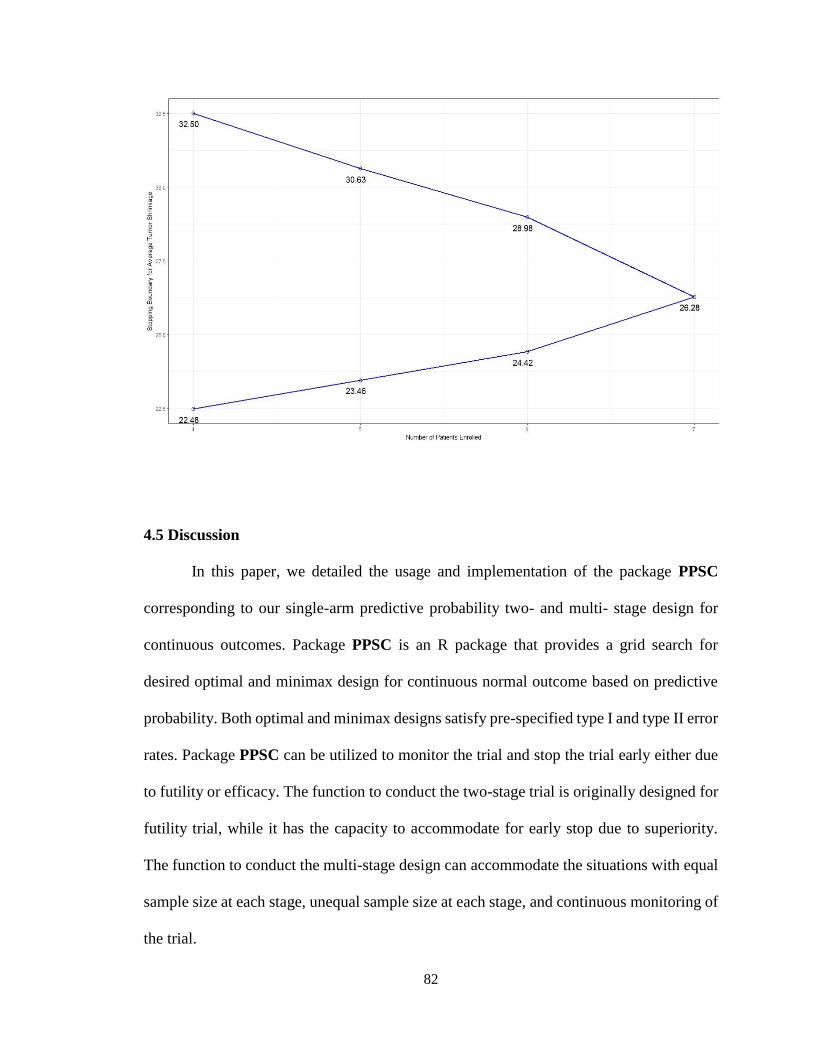
82

4.5 Discussion

In this paper, we detailed the usage and implementation of the package PPSC

corresponding to our single-arm predictive probability two- and multi- stage design for

continuous outcomes. Package PPSC is an R package that provides a grid search for

desired optimal and minimax design for continuous normal outcome based on predictive

probability. Both optimal and minimax designs satisfy pre-specified type I and type II error

rates. Package PPSC can be utilized to monitor the trial and stop the trial early either due

to futility or efficacy. The function to conduct the two-stage trial is originally designed for

futility trial, while it has the capacity to accommodate for early stop due to superiority.

The function to conduct the multi-stage design can accommodate the situations with equal

sample size at each stage, unequal sample size at each stage, and continuous monitoring of

the trial.

83

On the other hand, there are several limitations to the current version of Package

PPSC. First, Package PPSC is currently available only for normally distributed outcomes

with conjugated priors. Second, in terms of multi-stage design, especially for the purpose

of continuous monitoring, this version can only incorporate up to 40 stages due to the

current package R2Cuba for multidimensional numerical integration [77]. Third, for two-

stage design, the package PPSC yields both optimal design and minimax design in the

output. A user-defined range for 𝑃𝑇 and 𝑃𝐿 is searched to find both optimal and minimax

designs. However, only minimax design is shown for multi-stage setting, due to the grid

searching strategy and algorithm we employed. In the multi-stage setting, we restrict 𝑃𝐿

and 𝑃𝑈 as a user-defined value and search for a user-defined range for 𝑃𝑇 to find the

minimax design.

In summary, we extended Lee and Liu’s predictive probability approach into two-

stage and multi-stage setting for continuous endpoints. In practice, these two designs are

more relevant for treatment effects with short observation time. In the scenario where the

treatment effect will take a long period, such as several weeks or months, to observe, this

design is not quite useful. That is when the long-time treatment effect is expected in

practice, patients will have been enrolled in later stages in the trial, since the patients will

generally recruited continuously. Of course, it also depends on the institutes and recourses

to enroll patients. We also developed an R package PPSC to implement the described

designs. This package will be submitted to CRAN shortly after completion of this study

and will then be freely accessible in R. All necessary functions are available upon request.

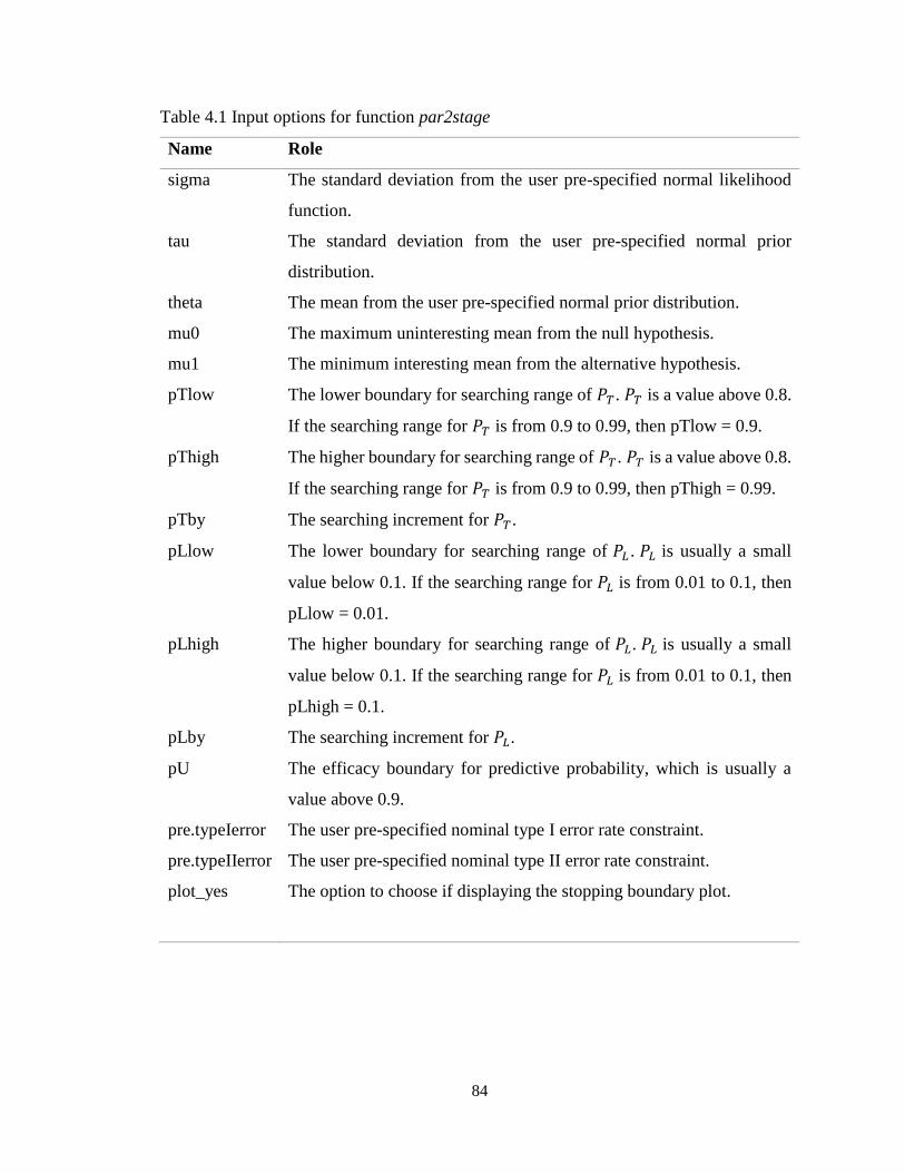
84

Table 4.1 Input options for function par2stage

Name Role

sigma The standard deviation from the user pre-specified normal likelihood

function.

tau The standard deviation from the user pre-specified normal prior

distribution.

theta The mean from the user pre-specified normal prior distribution.

mu0 The maximum uninteresting mean from the null hypothesis.

mu1 The minimum interesting mean from the alternative hypothesis.

pTlow The lower boundary for searching range of 𝑃𝑇. 𝑃𝑇 is a value above 0.8.

If the searching range for 𝑃𝑇 is from 0.9 to 0.99, then pTlow = 0.9.

pThigh The higher boundary for searching range of 𝑃𝑇. 𝑃𝑇 is a value above 0.8.

If the searching range for 𝑃𝑇 is from 0.9 to 0.99, then pThigh = 0.99.

pTby The searching increment for 𝑃𝑇 .

pLlow The lower boundary for searching range of 𝑃𝐿 . 𝑃𝐿 is usually a small

value below 0.1. If the searching range for 𝑃𝐿 is from 0.01 to 0.1, then

pLlow = 0.01.

pLhigh The higher boundary for searching range of 𝑃𝐿. 𝑃𝐿 is usually a small

value below 0.1. If the searching range for 𝑃𝐿 is from 0.01 to 0.1, then

pLhigh = 0.1.

pLby The searching increment for 𝑃𝐿.

pU The efficacy boundary for predictive probability, which is usually a

value above 0.9.

pre.typeIerror The user pre-specified nominal type I error rate constraint.

pre.typeIIerror The user pre-specified nominal type II error rate constraint.

plot_yes The option to choose if displaying the stopping boundary plot.

85

Table 4.2 Input options for function parmultistage

Name Role

continuous The option to choose continuous monitoring or not. The default value

is F.

first.look The proportion of the total sample for the first interim look. The default

value is NULL. The user should specify a number when continuously

monitoring is desired.

num.interim The number of interim looks during the trial.

equal.space The option to set equally spaced interim looks. The default value is T.

user.p The user defined proportion of sample size for each interim looks.

sigma The standard deviation from the user pre-specified normal likelihood

function.

tau The standard deviation from the user pre-specified normal prior

distribution.

theta The mean from the user pre-specified normal prior distribution.

mu0 The maximum uninteresting mean from the null hypothesis.

mu1 The minimum interesting mean from the alternative hypothesis.

pTlow The lower boundary for searching range of 𝑃𝑇. 𝑃𝑇 is a value above 0.8.

If the searching range for 𝑃𝑇 is from 0.9 to 0.99, then pTlow = 0.9.

pThigh The higher boundary for searching range of 𝑃𝑇. 𝑃𝑇 is a value above 0.8.

If the searching range for 𝑃𝑇 is from 0.9 to 0.99, then pThigh = 0.99.

pTby The searching increment for 𝑃𝑇 .

pL The user pre-specified value for 𝑃𝐿 , which is usually a small value

below 0.1.

pU The user pre-specified value for 𝑃𝑈 , which is usually a large value

above 0.9.

pre.typeIerror The user pre-specified nominal type I error rate constraint.

pre.typeIIerror The user pre-specified nominal type II error rate constraint.

plot_yes The option to choose if displaying the stopping boundary plot.

86

CHAPTER FIVE

Summary and Conclusion

5.1 Conclusion

Phase II trials aim to identify promising agents or therapies to move forward to

confirmative randomized phase III trials. In practice, RECIST criteria is commonly applied

to categorize the tumor shrinkage into complete response, partial response, progressive

disease and stable disease [1]. Response rate, which is the combination of complete and

partial response, with at least a 30% decrease in the sum of the longest diameter of the

target lesions, is usually used as a secondary endpoint in most of the cancer trials. However,

as shown in the previous studies, this dichotomization not only leads to loss of statistical

efficiency, but greatly increases the required sample size [5, 54-56, 58].

Interim strategies are of great importance in each stage of oncology clinical trials,

and at least one interim look is usually encouraged when designing the trial. The

purpose of interim looks is to terminate the trial early for safety, futility, or efficacy,

and to facilitate the trial process and protect patients’ clinical benefits [14]. Two-stage

design is widely used in phase II trials, one of which is Simon’s two-stage design in a

single-arm setting for binary outcomes, such as response rate [19]. It has been extended

in many different ways and has been summarized in the introduction part. Regarding

multi-stage designs, the group-sequential approach is usually used in practice. A group-

sequential design for clinical trial is usually to analyze the interim data after groups of

patients are enrolled. In this scheme, the number of patients at each stage is pre-specified

and the trial continues as long as the underlying test statistics keeps within a specified

boundary. In the randomized setting, group sequential designs are well developed and

87

widely applied in practice to identify and select new therapies [62, 63, 74]. For single-arm

settings, in particular, Chang et al. proposed a group-sequential design for binary outcomes

with minimized average expected sample size under the null and alternative hypotheses in

phase II trials under the frequentist framework [80]. When compared with frequentist

designs, Bayesian designs are more flexible. Lee and Liu proposed a predictive probability

design, on which we developed our researches [37].

In this dissertation, we proposed a two-stage design and a multi-stage design for

continuous endpoints based on predictive probability and developed an R package for these

two designs. The two-stage design is mainly focused on futility early termination while it

has the capacity to stop for efficacy. The multi-stage design has the flexibility to allow

early stopping either due to futility or efficacy. Both designs are flexible and user-friendly.

The users can choose to monitor the trial continuously, or to monitor the trial with pre-

specified number of stages, in which the users have the options to set equal or unequal

proportions of patients at each stage. Both designs meet pre-specified type I and type II

error rate constraints.

For both design options, we obtained similar decreased sample size as in previous

studies, when using tumor shrinkage instead of response rate, as continuous variable and

maintained the frequentist operating characteristics at the same time [5, 56]. We also

explored and evaluated the roles of priors on the effect of the design operating

characteristics. The results were shown to be fairly robust, although the comparison was

illustrative but not conclusive. Assessed priors yielded similar sample sizes and other

operating characteristics were slightly different. We also compared our results with designs

based on posterior designs, and the results were very similar. However, when compared

88

with posterior probability design, this predictive probability approach has the advantages

that it mimics the decision making process in reality and more intuitive. It answers the

question that if additional data are collected, is the trial likely to show convincing evidence

against the null hypothesis and in favor of the alternative hypothesis. The predictive

probabilities approach is able to model the endpoint using earlier information that is

informative about the final outcome.

5.2 Strength and Limitations

Strengths:

In general, multi-stage is usually more efficient than two-stage or three-stage design.

It is more efficient to stop the trial early for futility or superiority, which will save resources,

protect patients, and accelerate the process of drug development. When compared with

designs using binary outcomes, using continuous endpoints utilize more information from

the data and, therefore, reduce the sample size. Both of our designs based on predictive

probability, while maintaining the frequentist operating characteristics.

One of the major strengths for this study is the flexibility to implement and making

it an appealing alternative to other designs. In terms of two-stage design, the users have the

option to stop the trial early only due to futility, or to stop the trial early due to efficacy

with a specific value of 𝑃𝑇 . Regarding the multi-stage design, it allows continuous

monitoring up to 40 stages. It is particularly useful when the effect size is large, and the

investigators want to monitor the trial continuously. Further, this multi-stage design allows

the flexibility of setting either equal or unequal numbers of patients at each stage when the

effect size is moderate or small. To choose the design with equal numbers of patients at

89

each stage, the users just need to specify the number of interim looks they prefer. On the

other side, if the users would like designs with unequal sample size for each stages, they

can specify the cumulative proportion of the total sample size at each interim look.

Another strength for this current study is that although the trial stopping boundaries

are obtained from the predictive probability given the information from current data, which

resembles more closely to the decision making process of conducting clinical trials in

practice, it relies on parameters 𝑃𝐿, 𝑃𝑈 and 𝑃𝑇 to control the type I and type II error rate

constraints in the meanwhile. With this hybrid setting, our designs were shown to possess

the desirable operating characteristics and maintain both type I and type II error rates.

Further, it has been shown that our design gave fairly robust results across different

priors. The choice of priors is important in Bayesian clinical trial designs. We compared

the results across “weak/strong” and “optimistic/ pessimistic” priors and all the results were

very similar across different prior combinations, although more thorough assessment of

priors’ effect, especially those non-conjugated priors, should be conducted in the future.

Another strength is that we develop an R package PPSC to implement both two-

stage and multi-stage design. It is important to have a user-friendly tool available, which

makes the two designs accessible in the future for the collaboration between biostatisticians

and investigators.

Limitations:

There are several limitations in current two-stage and multi-stage designs, which

we plan to address in the future. Firstly, for both designs, we assume the standard deviation

𝜎 for the likelihood function of the studying continuous endpoint is known, in line with

previous studies. It is reasonable, since in practice this value could be obtained from

90

precious trials or preclinical studies. However, when there is little prior information is

available, especially for those novel drugs or biomarkers, it is not a valid assumption. Thus,

unknown variance may be explored in the future. Secondly, prior are important in Bayesian

clinical trial designs. It is always challenging and controversial to choose a suitable prior

on the parameter of interest. For both designs, we only assessed the conjugate priors for

the mean, assuming variance is known, and explored a little bit on the roles of pessimistic

and optimistic priors. There could be clinical situations where the prior does not follow a

normal distribution and thus the resulting posterior does not have a closed form. More

exploration is needed in this regard. We plan to look at other non-normal priors, such as

log-normal distributions in the future.

In terms of the multistage design, although our R package has the flexibility for

user-defined sample size for each interim look, we need to set the value of 𝑃𝐿 and 𝑃𝑈 and

only search for 𝑃𝑇 to find the desired design. In addition, we need to do a thorough

evaluation on how to space the interim looks to achieve the most desirable design and how

it will affect the design properties. Further, our grid searching strategy can only

accommodate minimax design due to computation time due to the grid search strategy we

employed. It will be interesting to see how the probability of early termination under the

null hypothesis and compare the expected sample size from the optimal design with the

smallest sample size desired.

5.3 Future Directions

We plan to extend this current study in different directions. There are several future

directions in common for both two-stage design and multi-stage designs. First, since

91

current design can only operate on conjugator priors based on normal likelihood, we would

like to extend both current two-stage design and multi-stage design to accommodate non-

conjugate priors. To do this, we will utilize the WinBUGS software and the R package

R2WinBUGS to handle non-conjugate priors [81, 82]. Further, we only explored situations

where the continuous outcome follows a normal distribution. However, as mentioned

above, it may not be realistic in practice. Thus, we plan to explore other distributions for

the continuous endpoints. Second, in practice, the likelihood variance may not be known

in advance, we would like to incorporate the likelihood variance as an unknown parameter

into the design. Third, the current design is best for the short-term endpoints, which can

be evaluated without affecting the continuous process of patients’ recruitment. However,

this design may not be appropriate for those endpoints that need longer time to be obtained

and evaluated. Recently, with the development of immunotherapy in oncology, there are

several proposed designs taking into the treatment lagged time effect for the survival

endpoints [83-85]. One future direction is to incorporate time factor or delayed treatment

effect into the design for the continuous endpoints. Another possible future direction is

evaluate this continuous endpoint and survival outcome simultaneously, which may be

more interesting in terms of clinical impact.

Lastly, we also plan to optimize and update the searching strategy in the future. For

the multi-stage design described in chapter 3, the current version only allows searching for

a range of 𝑃𝑇 for the minimax design. We would like to optimize the searching strategy to

allow 𝑃𝐿 and 𝑃𝑈 search as well as the optimal design output. In addition, due to the current

algorithm, we can only accommodate up to 40 stages during the trial due to the dependency

92

of the cubature package [77]. We would like to expand it into continuous monitoring

without limitation.

In conclusion, we developed two predictive probability interim designs for

continuous endpoints and an R package to implement in this dissertation. The two designs

are flexible and well preserve statistical properties. It provides an alternative option for

continuous endpoints when a single-arm design with flexible interim stopping is desired.

As research rapidly moves to incorporate more immunotherapies and targeted therapies,

these designs will accommodate new types of outcomes while allowing for flexible

stopping rules for futility and/or efficacy to continue optimizing trial resources and

prioritize agents with compelling early phase data.

93

APPENDICES

A1 Transformations from binary endpoints (𝒑) to continuous endpoints

(𝜇)[5] (From Wason et al., 2011).

Let 𝑝0 denote the response rate under the null hypothesis and 𝑝1 denote

the response rate under the alternative hypothesis. 𝜇0 is the tumor shrinkage

under the null hypothesis and 𝜇1 is under the alternative hypothesis. 𝜎 is the

standard deviation of the continuous endpoint, which is assumed to be known.

𝑑 is the cut-off the ratio of dichotomization, which is 30% with RECIST criteria

[1]. 𝑋 is denoted as the random variable for the continuous endpoint, such as

tumor shrinkage. 𝑍 is the standard normal random variable.

𝑝0 = Pr(𝑋 > 𝑑) = Pr(𝜎𝑍 + 𝜇0 > 𝑑) = 1 − 𝛷(𝑑 − 𝜇0

𝜎)

So that:

𝜇0 = 𝑑 − 𝜎𝛷−1(1 − 𝑝0)

Similarly,

𝜇1 = 𝑑 − 𝜎𝛷−1(1 − 𝑝1)

94

A2 Frequentist operating characteristics calculation for two-stage design

to terminate early for efficacy.

If the investigators prefer to terminating the trial early for both futility and efficacy, we

can rewrite the 𝜑(∙) in chapter one in the form of rejecting the null hypothesis at each

stage. We denote it as 𝜑∗(∙). Thus,

𝜑∗(𝜇0, 𝜎, 𝑛1 , 𝑛2 , �̅�𝑛1 , �̅�𝐿, �̅�𝑈, �̅�𝐿′) = 𝑃𝜇(�̅�𝑛1 ≥ �̅�𝑈) + ∫ 𝑓𝜇(𝑥)𝑃𝜇(�̅�𝑛1+𝑛2 ≥ �̅�𝑈

′ )�̅�𝑈

�̅�𝐿

𝑑𝑥

Similar as 𝜑(. ), the first part of 𝜑∗(. ) is the probability of rejecting the null hypothesis at

the first stage and the second part if the probability of rejecting the null at the end of

second stage.

The corresponding type I and type II error rates can be written as:

𝛼 = 𝜑∗(𝜇0, 𝜎, 𝑛1 , 𝑛2 , �̅�𝑛1 , �̅�𝐿, �̅�𝑈, �̅�𝐿′)

𝛽 = 1 − 𝜑∗(𝜇1, 𝜎, 𝑛1 , 𝑛2 , �̅�𝑛1 , �̅�𝐿 , �̅�𝑈, �̅�𝐿′)

The probability of early termination under the null hypothesis is :

𝑃𝐸𝑇(𝜇0) = 𝑃𝜇(�̅�𝑛1 ≤ �̅�𝐿|𝐻0) + 𝑃𝜇(�̅�𝑛1 ≥ �̅�𝑈|𝐻0)

And the expected sample size under the null hypothesis is the same as the situation for

only stopping early for futility.

95

A3 Supplementary simulation results for two-stage designs.

Table A3.1 Optimal two-stage design stopping early for futility

Table A3.2 Minimax two-stage design stopping early for futility

Table A3.3 Optimal two-stage design stopping early for efficacy

Table A3.4 Minimax two-stage design stopping early for efficacy

Table A3.5 Operating characteristics of optimal efficacy designs with different priors.

Table A3.6 Operating characteristics of minimax efficacy designs with different priors.

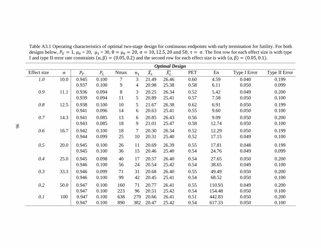
96

Table A3.1 Operating characteristics of optimal two-stage design for continuous endpoints with early termination for futility. For both

designs below, 𝑃𝑈 = 1, μ0 = 20, μ1 = 30, θ = μ0 = 20, σ = 10, 12.5, 20 and 50, τ = σ. The first row for each effect size is with type

I and type II error rate constraints (α, β) = (0.05, 0.2) and the second row for each effect size is with (α, β) = (0.05, 0.1).

Optimal Design

Effect size σ 𝑃𝑇 𝑃𝐿 Nmax 𝑛1 �̅�𝐿 �̅�𝐿′ PET En Type I Error Type II Error

1.0 10.0 0.945 0.100 7 3 21.49 26.46 0.60 4.59 0.040 0.199 0.937 0.100 9 4 20.98 25.38 0.58 6.11 0.050 0.099

0.9 11.1

11

0.936 0.094 8 3 20.25 26.34 0.52 5.42 0.049 0.200

0.939 0.094 11 5 20.89 25.41 0.57 7.58 0.050 0.100

0.8 12.5 0.938 0.100 10 5 21.67 26.38 0.62 6.91 0.050 0.199 0.941 0.096 14 6 20.63 25.41 0.55 9.60 0.050 0.100

0.7 14.3 0.941 0.085 13 6 20.85 26.43 0.56 9.09 0.050 0.200

0.943 0.085 18 9 21.01 25.47 0.58 12.74 0.050 0.100

0.6 16.7 0.942 0.100 18 7 20.30 26.34 0.52 12.29 0.050 0.199

0.944 0.099 25 10 20.31 25.40 0.52 17.15 0.049 0.100

0.5 20.0 0.945 0.100 26 11 20.69 26.39 0.55 17.81 0.048 0.199 0.945 0.100 36 15 20.46 25.40 0.54 24.76 0.049 0.099

0.4 25.0 0.945 0.098 40 17 20.57 26.40 0.54 27.65 0.050 0.200

0.946 0.100 56 24 20.54 25.42 0.54 38.65 0.049 0.100

0.3 33.3 0.946 0.099 71 31 20.68 26.40 0.55 49.49 0.050 0.200

0.946 0.100 99 42 20.45 25.41 0.54 68.52 0.050 0.100

0.2 50.0 0.947 0.100 160 71 20.77 26.41 0.55 110.93 0.049 0.200 0.947 0.100 223 96 20.51 25.42 0.54 154.48 0.050 0.100

0.1 100 0.947 0.100 638 279 20.66 26.41 0.51 442.83 0.050 0.200

0.947 0.100 890 382 20.47 25.42 0.54 617.33 0.050 0.100

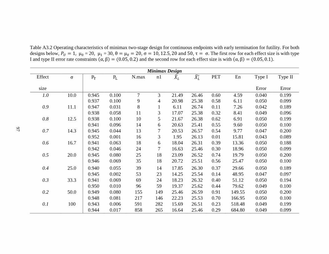
97

Table A3.2 Operating characteristics of minimax two-stage design for continuous endpoints with early termination for futility. For both

designs below, 𝑃𝑈 = 1, μ0 = 20, μ1 = 30, θ = μ0 = 20, σ = 10, 12.5, 20 and 50, τ = σ. The first row for each effect size is with type

I and type II error rate constraints (α, β) = (0.05, 0.2) and the second row for each effect size is with (α, β) = (0.05, 0.1).

Minimax Design

Effect

size

σ PT PL N.max n1 �̅�𝐿 �̅�𝐿′ PET En Type I

Error

Type II

Error

1.0 10.0 0.945 0.100 7 3 21.49 26.46 0.60 4.59 0.040 0.199

0.937 0.100 9 4 20.98 25.38 0.58 6.11 0.050 0.099

0.9 11.1

11

0.947 0.031 8 1 6.11 26.74 0.11 7.26 0.042 0.189

0.938 0.058 11 3 17.07 25.38 0.32 8.41 0.049 0.096

0.8 12.5 0.938 0.100 10 5 21.67 26.38 0.62 6.91 0.050 0.199

0.941 0.096 14 6 20.63 25.41 0.55 9.60 0.050 0.100

0.7 14.3 0.945 0.044 13 7 20.53 26.57 0.54 9.77 0.047 0.200

0.952 0.001 16 3 1.95 26.13 0.01 15.81 0.043 0.089

0.6 16.7 0.941 0.063 18 6 18.04 26.31 0.39 13.36 0.050 0.188

0.942 0.046 24 7 16.63 25.46 0.30 18.96 0.050 0.099

0.5 20.0 0.945 0.080 25 18 23.09 26.52 0.74 19.79 0.050 0.200

0.946 0.069 35 18 20.72 25.51 0.56 25.47 0.050 0.100

0.4 25.0 0.940 0.055 39 14 17.85 26.30 0.37 29.66 0.050 0.189

0.945 0.002 53 23 14.25 25.54 0.14 48.95 0.047 0.097

0.3 33.3 0.941 0.069 69 24 18.23 26.32 0.40 51.12 0.050 0.194

0.950 0.010 96 59 19.37 25.62 0.44 79.62 0.049 0.100

0.2 50.0 0.949 0.080 155 149 25.46 26.59 0.91 149.55 0.050 0.200

0.948 0.081 217 146 22.23 25.53 0.70 166.95 0.050 0.100

0.1 100 0.943 0.006 591 282 15.69 26.51 0.23 518.48 0.049 0.199

0.944 0.017 858 265 16.64 25.46 0.29 684.80 0.049 0.099

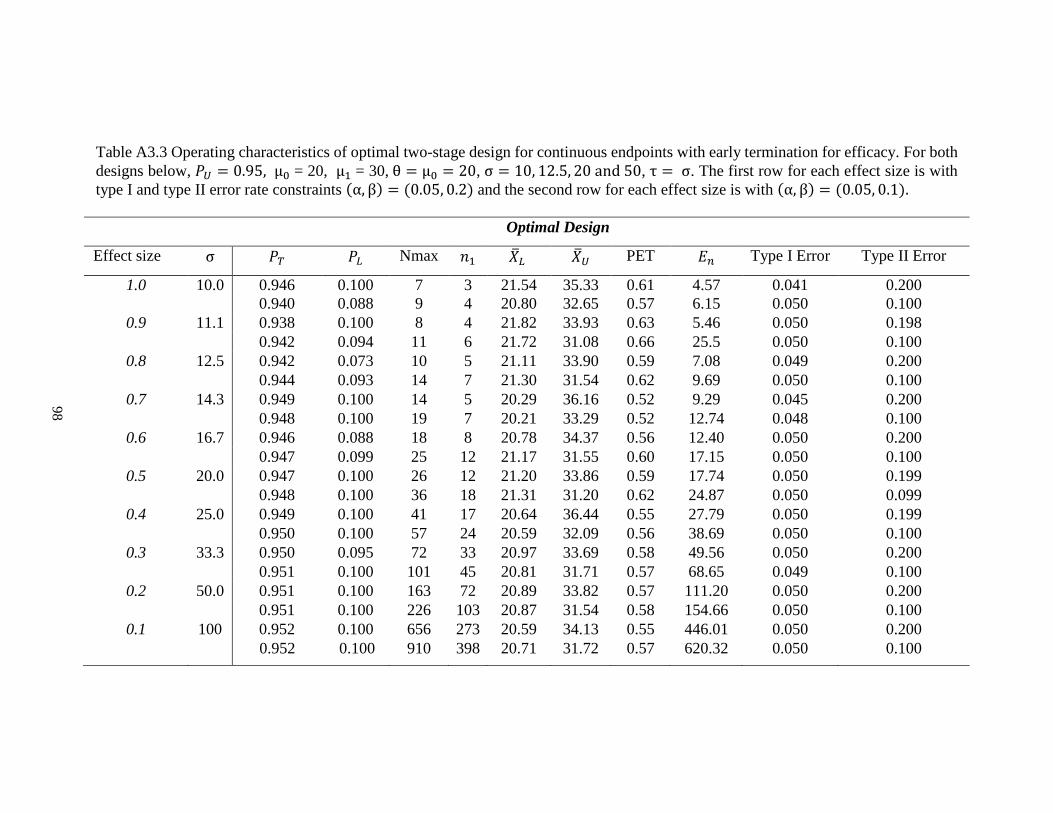
98

Table A3.3 Operating characteristics of optimal two-stage design for continuous endpoints with early termination for efficacy. For both

designs below, 𝑃𝑈 = 0.95, μ0 = 20, μ1 = 30, θ = μ0 = 20, σ = 10, 12.5, 20 and 50, τ = σ. The first row for each effect size is with

type I and type II error rate constraints (α, β) = (0.05, 0.2) and the second row for each effect size is with (α, β) = (0.05, 0.1).

Optimal Design

Effect size σ 𝑃𝑇 𝑃𝐿 Nmax 𝑛1 �̅�𝐿 �̅�𝑈 PET 𝐸𝑛 Type I Error Type II Error

1.0 10.0 0.946 0.100 7 3 21.54 35.33 0.61 4.57 0.041 0.200 0.940 0.088 9 4 20.80 32.65 0.57 6.15 0.050 0.100

0.9 11.1

11

0.938 0.100 8 4 21.82 33.93 0.63 5.46 0.050 0.198

0.942 0.094 11 6 21.72 31.08 0.66 25.5 0.050 0.100

0.8 12.5 0.942 0.073 10 5 21.11 33.90 0.59 7.08 0.049 0.200 0.944 0.093 14 7 21.30 31.54 0.62 9.69 0.050 0.100

0.7 14.3 0.949 0.100 14 5 20.29 36.16 0.52 9.29 0.045 0.200

0.948 0.100 19 7 20.21 33.29 0.52 12.74 0.048 0.100

0.6 16.7 0.946 0.088 18 8 20.78 34.37 0.56 12.40 0.050 0.200

0.947 0.099 25 12 21.17 31.55 0.60 17.15 0.050 0.100

0.5 20.0 0.947 0.100 26 12 21.20 33.86 0.59 17.74 0.050 0.199 0.948 0.100 36 18 21.31 31.20 0.62 24.87 0.050 0.099

0.4 25.0 0.949 0.100 41 17 20.64 36.44 0.55 27.79 0.050 0.199

0.950 0.100 57 24 20.59 32.09 0.56 38.69 0.050 0.100

0.3 33.3 0.950 0.095 72 33 20.97 33.69 0.58 49.56 0.050 0.200

0.951 0.100 101 45 20.81 31.71 0.57 68.65 0.049 0.100

0.2 50.0 0.951 0.100 163 72 20.89 33.82 0.57 111.20 0.050 0.200 0.951 0.100 226 103 20.87 31.54 0.58 154.66 0.050 0.100

0.1 100 0.952 0.100 656 273 20.59 34.13 0.55 446.01 0.050 0.200

0.952 0.100

0.`00

910 398 20.71 31.72 0.57 620.32 0.050 0.100

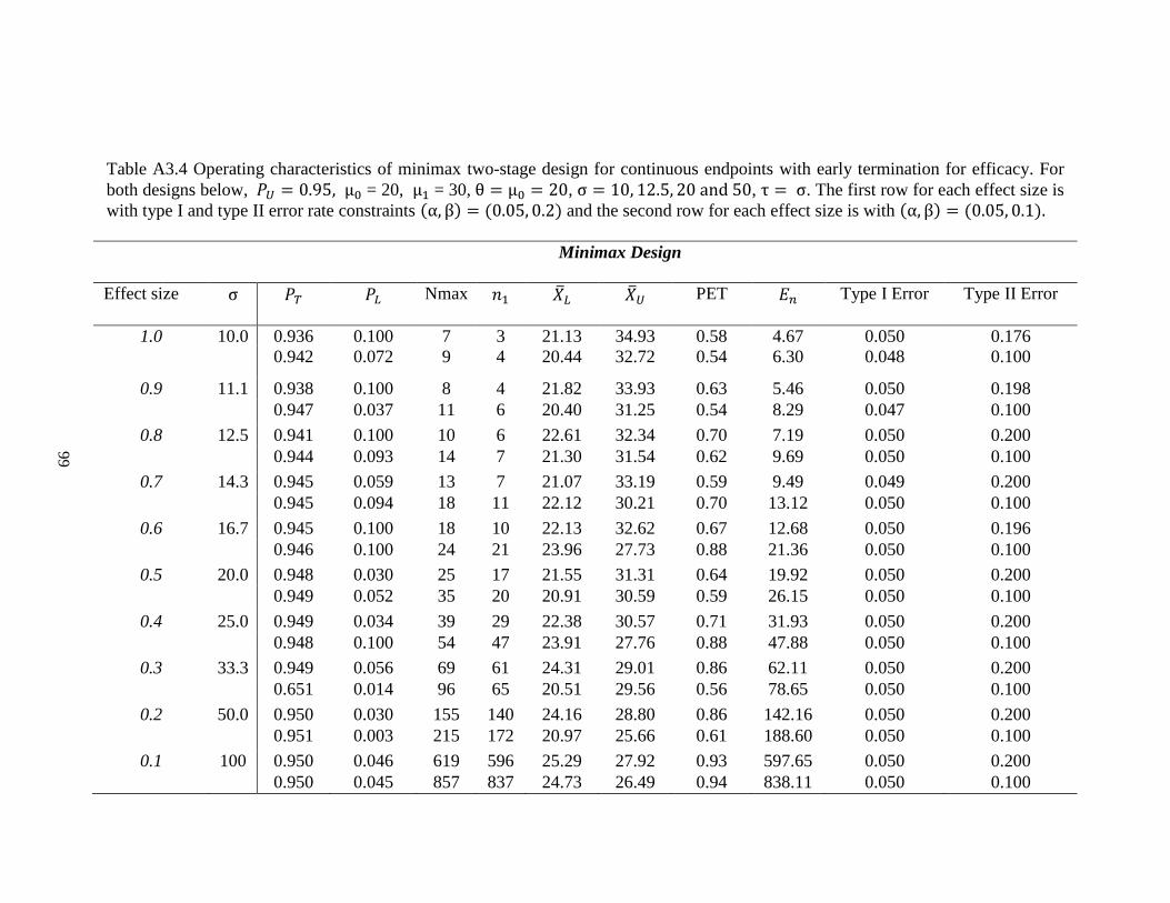
99

Table A3.4 Operating characteristics of minimax two-stage design for continuous endpoints with early termination for efficacy. For

both designs below, 𝑃𝑈 = 0.95, μ0 = 20, μ1 = 30, θ = μ0 = 20, σ = 10, 12.5, 20 and 50, τ = σ. The first row for each effect size is

with type I and type II error rate constraints (α, β) = (0.05, 0.2) and the second row for each effect size is with (α, β) = (0.05, 0.1).

Minimax Design

Effect size σ 𝑃𝑇 𝑃𝐿 Nmax 𝑛1 �̅�𝐿 �̅�𝑈 PET 𝐸𝑛 Type I Error Type II Error

1.0 10.0 0.936 0.100 7 3 21.13 34.93 0.58 4.67 0.050 0.176 0.942 0.072 9 4 20.44 32.72 0.54 6.30 0.048 0.100

0.9 11.1

11

0.938 0.100 8 4 21.82 33.93 0.63 5.46 0.050 0.198

0.947 0.037 11 6 20.40 31.25 0.54 8.29 0.047 0.100

0.8 12.5 0.941 0.100 10 6 22.61 32.34 0.70 7.19 0.050 0.200 0.944 0.093 14 7 21.30 31.54 0.62 9.69 0.050 0.100

0.7 14.3 0.945 0.059 13 7 21.07 33.19 0.59 9.49 0.049 0.200

0.945 0.094 18 11 22.12 30.21 0.70 13.12 0.050 0.100

0.6 16.7 0.945 0.100 18 10 22.13 32.62 0.67 12.68 0.050 0.196

0.946 0.100 24 21 23.96 27.73 0.88 21.36 0.050 0.100

0.5 20.0 0.948 0.030 25 17 21.55 31.31 0.64 19.92 0.050 0.200 0.949 0.052 35 20 20.91 30.59 0.59 26.15 0.050 0.100

0.4 25.0 0.949 0.034 39 29 22.38 30.57 0.71 31.93 0.050 0.200

0.948 0.100 54 47 23.91 27.76 0.88 47.88 0.050 0.100

0.3 33.3 0.949 0.056 69 61 24.31 29.01 0.86 62.11 0.050 0.200

0.651 0.014 96 65 20.51 29.56 0.56 78.65 0.050 0.100

0.2 50.0 0.950 0.030 155 140 24.16 28.80 0.86 142.16 0.050 0.200 0.951 0.003 215 172 20.97 25.66 0.61 188.60 0.050 0.100

0.1 100 0.950 0.046 619 596 25.29 27.92 0.93 597.65 0.050 0.200

0.950 0.045 857 837 24.73 26.49 0.94 838.11 0.050 0.100

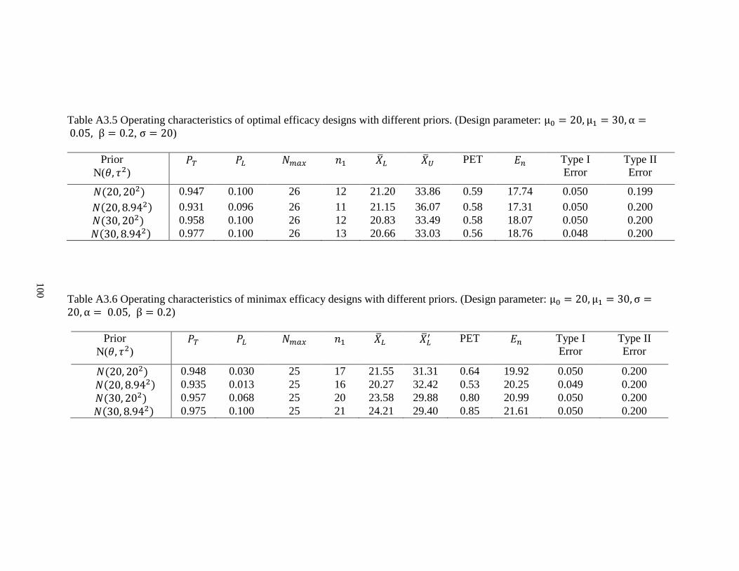
100

Table A3.5 Operating characteristics of optimal efficacy designs with different priors. (Design parameter: μ0 = 20, μ1 = 30, α = 0.05, β = 0.2, σ = 20)

Prior

N(𝜃, 𝜏2)

𝑃𝑇 𝑃𝐿 𝑁𝑚𝑎𝑥 𝑛1 �̅�𝐿 �̅�𝑈 PET 𝐸𝑛 Type I

Error

Type II

Error

𝑁(20, 202) 0.947 0.100 26 12 21.20 33.86 0.59 17.74 0.050 0.199

𝑁(20, 8.942) 0.931 0.096 26 11 21.15 36.07 0.58 17.31 0.050 0.200

𝑁(30, 202) 0.958 0.100 26 12 20.83 33.49 0.58 18.07 0.050 0.200

𝑁(30, 8.942) 0.977 0.100 26 13 20.66 33.03 0.56 18.76 0.048 0.200

Table A3.6 Operating characteristics of minimax efficacy designs with different priors. (Design parameter: μ0 = 20, μ1 = 30, σ =20, α = 0.05, β = 0.2)

Prior

N(𝜃, 𝜏2)

𝑃𝑇 𝑃𝐿 𝑁𝑚𝑎𝑥 𝑛1 �̅�𝐿 �̅�𝐿′ PET 𝐸𝑛 Type I

Error

Type II

Error

𝑁(20, 202) 0.948 0.030 25 17 21.55 31.31 0.64 19.92 0.050 0.200

𝑁(20, 8.942) 0.935 0.013 25 16 20.27 32.42 0.53 20.25 0.049 0.200

𝑁(30, 202) 0.957 0.068 25 20 23.58 29.88 0.80 20.99 0.050 0.200

𝑁(30, 8.942) 0.975 0.100 25 21 24.21 29.40 0.85 21.61 0.050 0.200

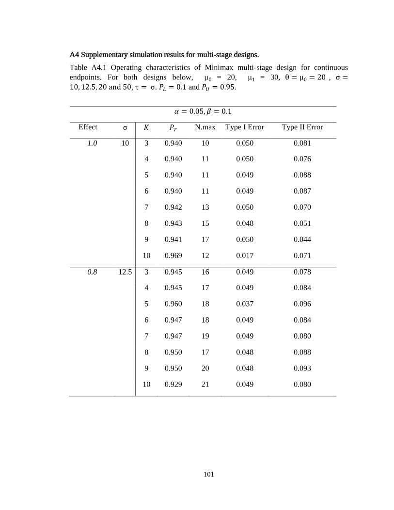
101

A4 Supplementary simulation results for multi-stage designs.

Table A4.1 Operating characteristics of Minimax multi-stage design for continuous

endpoints. For both designs below, μ0 = 20, μ1 = 30, θ = μ0 = 20 , σ =

10, 12.5, 20 and 50, τ = σ. 𝑃𝐿 = 0.1 and 𝑃𝑈 = 0.95.

𝛼 = 0.05, 𝛽 = 0.1

Effect

size

σ 𝐾 𝑃𝑇 N.max Type I Error Type II Error

1.0 10 3 0.940 10 0.050 0.081

4 0.940 11 0.050 0.076

5 0.940 11 0.049 0.088

6 0.940 11 0.049 0.087

7 0.942 13 0.050 0.070

8 0.943 15 0.048 0.051

9 0.941 17 0.050 0.044

10 0.969 12 0.017 0.071

0.8 12.5 3 0.945 16 0.049 0.078

4 0.945 17 0.049 0.084

5 0.960 18 0.037 0.096

6 0.947 18 0.049 0.084

7 0.947 19 0.049 0.080

8 0.950 17 0.048 0.088

9 0.950 20 0.048 0.093

10 0.929 21 0.049 0.080

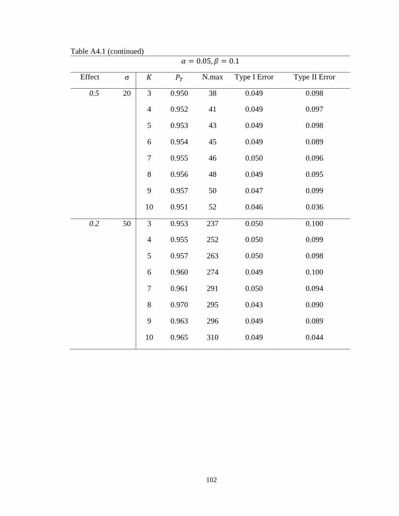
102

Table A4.1 (continued)

𝛼 = 0.05, 𝛽 = 0.1

Effect

size

σ 𝐾 𝑃𝑇 N.max Type I Error Type II Error

0.5 20 3 0.950 38 0.049 0.098

4 0.952 41 0.049 0.097

5 0.953 43 0.049 0.098

6 0.954 45 0.049 0.089

7 0.955 46 0.050 0.096

8 0.956 48 0.049 0.095

9 0.957 50 0.047 0.099

10 0.951 52 0.046 0.036

0.2 50 3 0.953 237 0.050 0.100

4 0.955 252 0.050 0.099

5 0.957 263 0.050 0.098

6 0.960 274 0.049 0.100

7 0.961 291 0.050 0.094

8 0.970 295 0.043 0.090

9 0.963 296 0.049 0.089

10 0.965 310 0.049 0.044

103

A5. Calculation of covariance between �̅�𝒏𝒊 and �̅�𝒏𝒋:

Let 𝑛𝑖 denote the cumulative number of patients at ith stage and 𝑛𝑗 denote the cumulative

sample size at jth stage, where 𝑛𝑗 > 𝑛𝑖. Thus, �̅�𝑛𝑖 denotes the average tumor shrinkage

from the 𝑛𝑖 patients and �̅�𝑛𝑗 denotes the average tumor shrinkage from the 𝑛𝑗 patients.

𝐶𝑜𝑣(�̅�𝑛𝑖 , �̅�𝑛𝑗) = 𝐶𝑜𝑣 (1

𝑛𝑖∑ 𝑋𝑖𝑛𝑖𝑖=1 ,

1

𝑛𝑗∑ 𝑋𝑗𝑛𝑗𝑗=1

)

= 𝐸(1

𝑛𝑖∑𝑋𝑖

𝑛𝑖

𝑖=1

∗ 1

𝑛𝑗∑𝑋𝑗

𝑛𝑗

𝑗=1

) − 𝐸 (1

𝑛𝑖∑𝑋𝑖

𝑛𝑖

𝑖=1

)𝐸 (1

𝑛𝑗∑𝑋𝑗

𝑛𝑗

𝑗=1

)

=1

𝑛𝑖𝑛𝑗 𝐸 (∑ 𝑋𝑖

𝑛𝑖𝑖=1

∑ 𝑋𝑗𝑛𝑗𝑗=1

) − 𝜇2

=1

𝑛𝑖𝑛𝑗𝐸 (𝑛𝑖�̅�𝑛𝑖𝑛𝑗�̅�𝑛𝑗) − 𝜇

2

= 1

𝑛𝑖𝑛𝑗𝐸 [𝑛𝑖�̅�𝑛𝑖 ∗ (𝑛𝑖�̅�𝑛𝑖 + (𝑛𝑗 − 𝑛𝑖 )�̅�′𝑛𝑗)] − 𝜇

2

=1

𝑛𝑖𝑛𝑗𝐸 [𝑛𝑖

2�̅�𝑛𝑖2 + 𝑛𝑖�̅�𝑛𝑖(𝑛𝑗 − 𝑛𝑖 )�̅�𝑛𝑗

′ ] − 𝜇2

=𝑛𝑖2

𝑛𝑖𝑛𝑗𝐸[�̅�𝑛𝑖

2 ] + 𝑛𝑖(𝑛𝑗 − 𝑛𝑖 )

𝑛𝑖𝑛𝑗𝐸(�̅�𝑛𝑖�̅�𝑛𝑗

′ ) − 𝜇2

Since 𝐸[�̅�𝑛𝑖2 ] = 𝑉𝑎𝑟(�̅�𝑛𝑖) + [𝐸(�̅�𝑛𝑖)]

2, �̅�𝑛𝑖 and �̅�𝑛𝑗′ are independent with both mean 𝜇,

where �̅�𝑛𝑗′ is the average tumor shrinkage from the patients 𝑛𝑗 − 𝑛𝑖.

𝐶𝑜𝑣(�̅�𝑛𝑖 , �̅�𝑛𝑗) = 𝑛𝑖2

𝑛𝑖𝑛𝑗(𝑉𝑎𝑟(�̅�𝑛𝑖) + [𝐸(�̅�𝑛𝑖)]

2) + 𝑛𝑖(𝑛𝑗−𝑛𝑖 )

𝑛𝑖𝑛𝑗𝐸(�̅�𝑛𝑖)𝐸 (�̅�𝑛𝑗

′ ) − 𝜇2

=𝑛𝑖2

𝑛𝑖𝑛𝑗(𝜎2

𝑛𝑖+ 𝜇2 ) +

𝑛𝑖(𝑛𝑗−𝑛𝑖 )

𝑛𝑖𝑛𝑗 𝜇2 − 𝜇2

104

= 𝜎2

𝑛𝑗+𝑛𝑖2

𝑛𝑖𝑛𝑗𝜇2 + 𝜇2 −

𝑛𝑖2

𝑛𝑖𝑛𝑗𝜇2 − 𝜇2 =

𝜎2

𝑛𝑗

Calculation of covariance between 𝒁𝒏𝒊 and 𝒁𝒏𝒋 from �̅�𝒏𝒊 and �̅�𝒏𝒋

𝑍𝑛𝑖 = �̅�𝑛𝑖− 𝜇

√𝜎2/𝑛𝑖 and 𝑍𝑛𝑗 =

�̅�𝑛𝑗− 𝜇

√𝜎2/𝑛𝑗

𝐶𝑜𝑣(𝑍𝑛𝑖 , 𝑍𝑛𝑗) = 𝐶𝑜𝑣

(

�̅�𝑛𝑖− 𝜇

√𝜎2

𝑛𝑖

, �̅�𝑛𝑗− 𝜇

√𝜎2

𝑛𝑗

)

= 𝐸

(

�̅�𝑛𝑖− 𝜇

√𝜎2

𝑛𝑖

∗�̅�𝑛𝑗− 𝜇

√𝜎2

𝑛𝑗

)

− 𝐸(

�̅�𝑛𝑖− 𝜇

√𝜎2

𝑛𝑖

)𝐸(�̅�𝑛𝑗− 𝜇

√𝜎2

𝑛𝑗

)

= √𝑛𝑖𝑛𝑗

𝜎2𝐸 [(�̅�𝑛𝑖 − 𝜇) (�̅�𝑛𝑗 − 𝜇)] −

√𝑛𝑖𝑛𝑗

𝜎2𝐸[�̅�𝑛𝑖 − 𝜇]𝐸 [�̅�𝑛𝑗 − 𝜇]

= √𝑛𝑖𝑛𝑗

𝜎2𝐸 [�̅�𝑛𝑖�̅�𝑛𝑗 − 𝜇 (�̅�𝑛𝑖 + �̅�𝑛𝑗) + 𝜇

2 ] − 0

= √𝑛𝑖𝑛𝑗

𝜎2𝐸 [�̅�𝑛𝑖�̅�𝑛𝑗] −

√𝑛𝑖𝑛𝑗

𝜎2𝐸 [𝜇 (�̅�𝑛𝑖 + �̅�𝑛𝑗)] +

√𝑛𝑖𝑛𝑗

𝜎2𝐸[𝜇2]

= √𝑛𝑖𝑛𝑗

𝜎2𝐸 [�̅�𝑛𝑖 ∗

1

𝑛𝑗∑𝑋𝑗

𝑛𝑗

𝑗=1

] −√𝑛𝑖𝑛𝑗

𝜎2𝐸 [𝜇 (�̅�𝑛𝑖 + �̅�𝑛𝑗)] +

√𝑛𝑖𝑛𝑗

𝜎2𝐸[𝜇2]

= √𝑛𝑖𝑛𝑗

𝜎21

𝑛𝑗𝐸 [�̅�𝑛𝑖 (𝑛𝑖�̅�𝑛𝑖 + (𝑛𝑗 − 𝑛𝑖 )�̅�′𝑛𝑗)] −

√𝑛𝑖𝑛𝑗

𝜎2𝐸 [𝜇 (�̅�𝑛𝑖 + �̅�𝑛𝑗)]

+√𝑛𝑖𝑛𝑗

𝜎2𝐸[𝜇2]

=1

𝜎2√𝑛𝑖𝑛𝑗𝐸 [𝑛𝑖�̅�𝑛𝑖

2 + (𝑛𝑗 − 𝑛𝑖 )�̅�𝑛𝑖�̅�′𝑛𝑗 ] − √𝑛𝑖𝑛𝑗

𝜎2𝜇𝐸 [�̅�𝑛𝑖 + �̅�𝑛𝑗] +

√𝑛𝑖𝑛𝑗

𝜎2 𝜇2

105

=𝑛𝑖𝜎2√𝑛𝑖𝑛𝑗 𝐸[�̅�𝑛𝑖

2 ] +1

𝜎2√𝑛𝑖𝑛𝑗𝐸 [(𝑛𝑗 − 𝑛𝑖 )�̅�𝑛𝑖�̅�′𝑛𝑗] − 2

√𝑛𝑖𝑛𝑗

𝜎2𝜇2 +

√𝑛𝑖𝑛𝑗

𝜎2 𝜇2

=𝑛𝑖𝜎2√𝑛𝑖𝑛𝑗 (𝑉𝑎𝑟(�̅�𝑛𝑖) + [𝐸(�̅�𝑛𝑖)]

2) +

1

𝜎2√𝑛𝑖𝑛𝑗(𝑛𝑗 − 𝑛𝑖 )𝐸 [�̅�𝑛𝑖�̅�′𝑛𝑗]

− √𝑛𝑖𝑛𝑗

𝜎2 𝜇2

= 𝑛𝑖

𝜎2√𝑛𝑖

𝑛𝑗(𝜎2

𝑛𝑖+ 𝜇2) +

1

𝜎2√𝑛𝑖

𝑛𝑗(𝑛𝑗 − 𝑛𝑖 )𝐸 [�̅�𝑛𝑖�̅�′𝑛𝑗] −

√𝑛𝑖𝑛𝑗

𝜎2 𝜇2

= √𝑛𝑖𝑛𝑗+ 𝑛𝑖𝜎2√𝑛𝑖𝑛𝑗𝜇2 +

√𝑛𝑖𝑛𝑗

𝜎2𝑛𝑗 𝜇

2 − 𝑛𝑖𝜎2√𝑛𝑖𝑛𝑗 𝜇2 −

√𝑛𝑖𝑛𝑗

𝜎2 𝜇2 = √

𝑛𝑖𝑛𝑗

Calculation of covariance between �̅�𝒏𝒊 and �̅�𝒏𝒋 from 𝒁𝒏𝒊 and 𝒁𝒏𝒋

Since 𝑍𝑛𝑖 = �̅�𝑛𝑖− 𝜇

√𝜎2/𝑛𝑖 and 𝑍𝑛𝑗 =

�̅�𝑛𝑗− 𝜇

√𝜎2/𝑛𝑗

, �̅�𝑛𝑖 = 𝑍𝑛𝑖√𝜎2/𝑛𝑖 + 𝜇 and �̅�𝑛𝑗 = 𝑍𝑛𝑗√𝜎

2/𝑛𝑗 +

𝜇

𝐶𝑜𝑣(�̅�𝑛𝑖 , �̅�𝑛𝑗) = 𝐶𝑜𝑣 (𝑍𝑛𝑖√𝜎2/𝑛𝑖 + 𝜇 , 𝑍𝑛𝑗√𝜎

2/𝑛𝑗 + 𝜇 )

= 𝐶𝑜𝑣 (𝑍𝑛𝑖√𝜎2

𝑛𝑖 , 𝑍𝑛𝑗√

𝜎2

𝑛𝑗 )

=𝜎2

√𝑛𝑖𝑛𝑗 𝐶𝑜𝑣 (𝑍𝑛𝑖 , 𝑍𝑛𝑗)

=𝜎2

√𝑛𝑖𝑛𝑗√𝑛𝑖

𝑛𝑗=𝜎2

𝑛𝑗

Package ‘PPSC’

July 17, 2017

Type Package

Title PPSC: An R Package for Single-Arm Phase II Trial Design with Continuous Endpoints based on Predictive Probability

Version 0.1.0

Author Meng LiuEmily V. Dressler

Maintainer Meng Liu <mengliu236@gmail.com>

Description This is an R package to implement the grid search of optimal and minimax de-signs for continuous endpoints based on predictive probability while meeting both user pre-specified type I and type II error rate constaints.

Depends cubature,R2Cuba,ggplot2

Imports cubature,R2Cuba,ggplot2

License GPL-2

Encoding UTF-8

LazyData true

Suggests knitr

RoxygenNote 6.0.1.9000

R topics documented:

par2stage . . . . . . . . . . . . . . . . . . . . . . . . . . . . . . . . . . . . . . . . . . 2parmultistage . . . . . . . . . . . . . . . . . . . . . . . . . . . . . . . . . . . . . . . . 3

Index 6

106

A6. R Package Manual

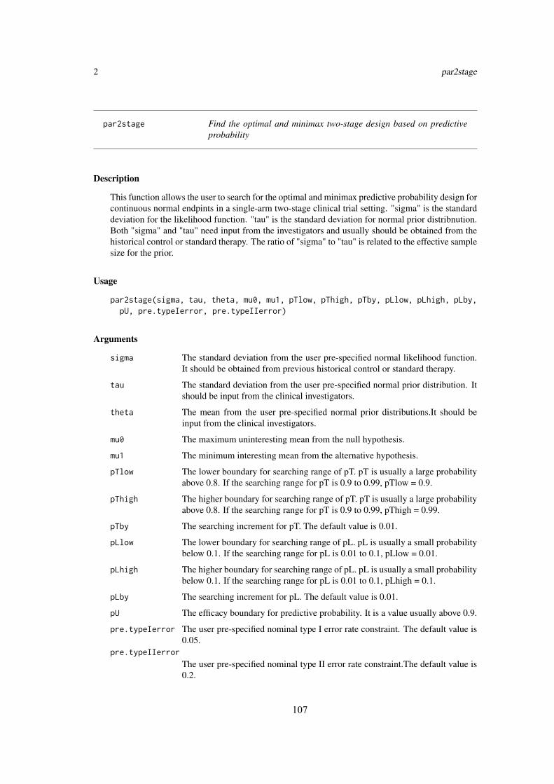
2 par2stage

par2stage Find the optimal and minimax two-stage design based on predictiveprobability

Description

This function allows the user to search for the optimal and minimax predictive probability design forcontinuous normal endpints in a single-arm two-stage clinical trial setting. "sigma" is the standarddeviation for the likelihood function. "tau" is the standard deviation for normal prior distribnution.Both "sigma" and "tau" need input from the investigators and usually should be obtained from thehistorical control or standard therapy. The ratio of "sigma" to "tau" is related to the effective samplesize for the prior.

Usage

par2stage(sigma, tau, theta, mu0, mu1, pTlow, pThigh, pTby, pLlow, pLhigh, pLby,pU, pre.typeIerror, pre.typeIIerror)

Arguments

sigma The standard deviation from the user pre-specified normal likelihood function.It should be obtained from previous historical control or standard therapy.

tau The standard deviation from the user pre-specified normal prior distribution. Itshould be input from the clinical investigators.

theta The mean from the user pre-specified normal prior distributions.It should beinput from the clinical investigators.

mu0 The maximum uninteresting mean from the null hypothesis.

mu1 The minimum interesting mean from the alternative hypothesis.

pTlow The lower boundary for searching range of pT. pT is usually a large probabilityabove 0.8. If the searching range for pT is 0.9 to 0.99, pTlow = 0.9.

pThigh The higher boundary for searching range of pT. pT is usually a large probabilityabove 0.8. If the searching range for pT is 0.9 to 0.99, pThigh = 0.99.

pTby The searching increment for pT. The default value is 0.01.

pLlow The lower boundary for searching range of pL. pL is usually a small probabilitybelow 0.1. If the searching range for pL is 0.01 to 0.1, pLlow = 0.01.

pLhigh The higher boundary for searching range of pL. pL is usually a small probabilitybelow 0.1. If the searching range for pL is 0.01 to 0.1, pLhigh = 0.1.

pLby The searching increment for pL. The default value is 0.01.

pU The efficacy boundary for predictive probability. It is a value usually above 0.9.

pre.typeIerror The user pre-specified nominal type I error rate constraint. The default value is0.05.

pre.typeIIerror

The user pre-specified nominal type II error rate constraint.The default value is0.2.

107

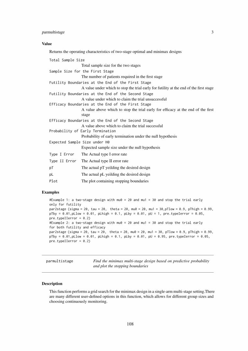
parmultistage 3

Value

Returns the operating characteristics of two-stage optimal and minimax designs

Total Sample Size

Total sample size for the two stagesSample Size for the First Stage

The number of patients required in the first stageFutility Boundaries at the End of the First Stage

A value under which to stop the trial early for futility at the end of the first stageFutility Boundaries at the End of the Second Stage

A value under which to claim the trial unsuccessfulEfficacy Boundaries at the End of the First Stage

A value above which to stop the trial early for efficacy at the end of the firststage

Efficacy Boundaries at the End of the Second Stage

A value above which to claim the trial successfulProbability of Early Termination

Probability of early termination under the null hypothesisExpected Sample Size under H0

Expected sample size under the null hypothesis

Type I Error The Actual type I error rate

Type II Error The Actual type II error rate

pT The actual pT yeilding the desired design

pL The actual pL yeilding the desired design

Plot The plot containing stopping boundaries

Examples

#Example 1: a two-stage design with mu0 = 20 and mu1 = 30 and stop the trial earlyonly for futilitypar2stage (sigma = 20, tau = 20, theta = 20, mu0 = 20, mu1 = 30,pTlow = 0.9, pThigh = 0.99,pTby = 0.01,pLlow = 0.01, pLhigh = 0.1, pLby = 0.01, pU = 1, pre.typeIerror = 0.05,pre.typeIIerror = 0.2)#Example 2: a two-stage design with mu0 = 20 and mu1 = 30 and stop the trial earlyfor both futility and efficacypar2stage (sigma = 20, tau = 20, theta = 20, mu0 = 20, mu1 = 30, pTlow = 0.9, pThigh = 0.99,pTby = 0.01,pLlow = 0.01, pLhigh = 0.1, pLby = 0.01, pU = 0.95, pre.typeIerror = 0.05,pre.typeIIerror = 0.2)

parmultistage Find the minimax multi-stage design based on predictive probabilityand plot the stopping boundaries

Description

This function performs a grid search for the minimax design in a single-arm multi-stage setting.Thereare many different user-defined options in this function, which allows for different group sizes andchoosing continuously monitoring.

108

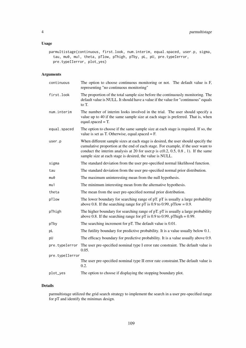
4 parmultistage

Usage

parmultistage(continuous, first.look, num.interim, equal.spaced, user.p, sigma,tau, mu0, mu1, theta, pTlow, pThigh, pTby, pL, pU, pre.typeIerror,pre.typeIIerror, plot_yes)

Arguments

continuous The option to choose continuous monitoring or not. The default value is F,representing "no continuous monitoring"

first.look The proportion of the total sample size before the continuously monitoring. Thedefault value is NULL. It should have a value if the value for "continuous" equalsto T.

num.interim The number of interim looks involved in the trial. The user should specify avalue up to 40 if the same sample size at each stage is preferred. That is, wheneqaul.spaced = T.

equal.spaced The option to choose if the same sample size at each stage is required. If so, thevalue is set as T. Otherwise, equal.spaced = F.

user.p When different sample sizes at each stage is desired, the user should specify thecumulative proportion at the end of each stage. For example, if the user want toconduct the interim analysis at 20 for user.p is c(0.2, 0.5, 0.8 , 1). If the samesample size at each stage is desired, the value is NULL.

sigma The standard deviation from the user pre-specified normal likelihood function.

tau The standard deviation from the user pre-specified normal prior distribution.

mu0 The maximum uninteresting mean from the null hypothesis.

mu1 The minimum interesting mean from the alternative hypothesis.

theta The mean from the user pre-specified normal prior distribution.

pTlow The lower boundary for searching range of pT. pT is usually a large probabilityabove 0.8. If the searching range for pT is 0.9 to 0.99, pTlow = 0.9.

pThigh The higher boundary for searching range of pT. pT is usually a large probabilityabove 0.8. If the searching range for pT is 0.9 to 0.99, pThigh = 0.99.

pTby The searching increment for pT. The default value is 0.01.

pL The futility boundary for predictive probability. It is a value usually below 0.1.

pU The efficacy boundary for predictive probability. It is a value usually above 0.9.

pre.typeIerror The user pre-specified nominal type I error rate constraint. The default value is0.05.

pre.typeIIerror

The user pre-specified nominal type II error rate constraint.The default value is0.2.

plot_yes The option to choose if displaying the stopping boundary plot.

Details

parmultistage utilized the grid search strategy to implement the search in a user pre-specified rangefor pT and identify the minimax design.

109

parmultistage 5

Value

Returns the operating characteristics of the minimax design

Cumulative sample size for each interim look

A vector containing the cumulative sample size at the end of each stage forinterim analysis

Futility Boundaries

A vector containing the futility stopping boundaries for each interim lookEfficacy Boundaries

A vector containing the efficacy stopping boundaries for each interim lookProbability of Early Termination

Probability of early termination under the null hypothesisExpected Sample Size under H0

Expected sample size under the null hypothesis

Type I Error The Actual type I error rate

Type II Error The Actual type II error rate

pT The actual pT yeilding the desired design

Plot The plot containing stopping boundaries

Examples

#Example 1 : Equal sample size at each interim lookparmultistage(continuous = F, first.look = NULL, num.interim = 2 , equal.spaced = T ,user.p = NULL, sigma = 20, tau = 20, mu0 = 20, mu1 = 30 , theta = 20, pTlow = 0.9,pThigh = 0.99, pTby = 0.01, pL = 0.1, pU = 0.95, pre.typeIerror = 0.05 ,pre.typeIIerror = 0.2, plot_yes = T)

#Example 2: Unequal sample size for at each interim lookparmultistage(continuous = F, first.look = NULL, num.interim = 3, equal.spaced = F ,user.p = c(0.1, 0.4, 0.8, 1.0),sigma = 20, tau = 20, mu0 = 20, mu1 = 30 , theta = 20,pTlow = 0.9, pThigh = 0.99, pTby = 0.01, pL = 0.1, pU = 0.95, pre.typeIerror = 0.05 ,pre.typeIIerror = 0.2, plot_yes = T)

#Exmaple 3: Continuouly monitor after 50% of sample size are enrolledparmultistage(continuous = T, first.look = 0.5, num.interim = NULL, equal.spaced = F ,user.p = NULL, sigma = 20, tau = 20, mu0 = 20, mu1 = 30 , theta = 20, pTlow = 0.9,pThigh = 0.99, pTby = 0.01, pL = 0.1, pU = 0.95, pre.typeIerror = 0.05 ,pre.typeIIerror = 0.2, plot_yes = T)

110

Index

∗Topic PPSCpar2stage, 2parmultistage, 3

par2stage, 2parmultistage, 3

111

112

BIBLIOGRAPHY

1. Eisenhauer, E.A., et al., New response evaluation criteria in solid tumours: revised

RECIST guideline (version 1.1). Eur J Cancer, 2009. 45(2): p. 228-47.

2. Adjei, A.A., M. Christian, and P. Ivy, Novel designs and end points for phase II

clinical trials. Clin Cancer Res, 2009. 15(6): p. 1866-72.

3. Seymour, L., et al., The design of phase II clinical trials testing cancer therapeutics:

consensus recommendations from the clinical trial design task force of the national

cancer institute investigational drug steering committee. Clin Cancer Res, 2010.

16(6): p. 1764-9.

4. Booth, C.M., et al., Design and conduct of phase II studies of targeted anticancer

therapy: recommendations from the task force on methodology for the development

of innovative cancer therapies (MDICT). Eur J Cancer, 2008. 44(1): p. 25-9.

5. Wason, J.M., A.P. Mander, and T.G. Eisen, Reducing sample sizes in two-stage

phase II cancer trials by using continuous tumour shrinkage end-points. Eur J

Cancer, 2011. 47(7): p. 983-9.

6. Altman, D.G. and P. Royston, The cost of dichotomising continuous variables. BMJ,

2006. 332(7549): p. 1080.

7. Claret, L., et al., Evaluation of tumor-size response metrics to predict overall

survival in Western and Chinese patients with first-line metastatic colorectal

cancer. J Clin Oncol, 2013. 31(17): p. 2110-4.

8. Delahunt, B., et al., Prognostic importance of tumor size for localized conventional

(clear cell) renal cell carcinoma: assessment of TNM T1 and T2 tumor categories

and comparison with other prognostic parameters. Cancer, 2002. 94(3): p. 658-64.

9. Simon, R., R.E. Wittes, and S.S. Ellenberg, Randomized phase II clinical trials.

Cancer Treat Rep, 1985. 69(12): p. 1375-81.

10. Rubinstein, L.V., et al., Design issues of randomized phase II trials and a proposal

for phase II screening trials. J Clin Oncol, 2005. 23(28): p. 7199-206.

11. Rosner, G.L., W. Stadler, and M.J. Ratain, Randomized discontinuation design:

application to cytostatic antineoplastic agents. J Clin Oncol, 2002. 20(22): p. 4478-

84.

12. Cannistra, S.A., Phase II trials in journal of clinical oncology. J Clin Oncol, 2009.

27(19): p. 3073-6.

13. Kamat, A.M., et al., Definitions, End Points, and Clinical Trial Designs for Non-

Muscle-Invasive Bladder Cancer: Recommendations From the International

Bladder Cancer Group. J Clin Oncol, 2016. 34(16): p. 1935-44.

14. Whitehead, J., Stopping clinical trials by design. Nat Rev Drug Discov, 2004. 3(11):

p. 973-7.

15. Emerson, S.S. and T.R. Fleming, Interim analyses in clinical trials. Oncology

(Williston Park), 1990. 4(3): p. 126-33; discussion 134, 136.

16. Fossa, S.D. and E. Skovlund, Interim analyses in clinical trials: why do we plan

them? J Clin Oncol, 2000. 18(24): p. 4007-8.

17. Whitehead, A., et al., Incorporating intermediate binary responses into interim

analyses of clinical trials: a comparison of four methods. Stat Med, 2008. 27(10):

p. 1646-66.

113

18. Gehan, E.A., The determinatio of the number of patients required in a preliminary

and a follow-up trial of a new chemotherapeutic agent. J Chronic Dis, 1961. 13: p.

346-53.

19. Simon, R., Optimal two-stage designs for phase II clinical trials. Control Clin

Trials, 1989. 10(1): p. 1-10.

20. Chen, T.T., Optimal three-stage designs for phase II cancer clinical trials. Stat

Med, 1997. 16(23): p. 2701-11.

21. Bryant, J. and R. Day, Incorporating toxicity considerations into the design of two-

stage phase II clinical trials. Biometrics, 1995. 51(4): p. 1372-83.

22. Conaway, M.R. and G.R. Petroni, Bivariate sequential designs for phase II trials.

Biometrics, 1995. 51(2): p. 656-64.

23. Jin, H., Alternative designs of phase II trials considering response and toxicity.

Contemp Clin Trials, 2007. 28(4): p. 525-31.

24. Lin, X., R. Allred, and G. Andrews, A two-stage phase II trial design utilizing both

primary and secondary endpoints. Pharm Stat, 2008. 7(2): p. 88-92.

25. Jung, S.H., M. Carey, and K.M. Kim, Graphical search for two-stage designs for

phase II clinical trials. Control Clin Trials, 2001. 22(4): p. 367-72.

26. Berry, D.A., Bayesian clinical trials. Nat Rev Drug Discov, 2006. 5(1): p. 27-36.

27. Spiegelhalter, D., et al., Bayesian methods in health technology assessment: a

review. Health Technology Assessment, 2000. 4(38): p. 130.

28. Thall, P.F. and R. Simon, Practical Bayesian guidelines for phase IIB clinical trials.

Biometrics, 1994. 50(2): p. 337-49.

29. Tan, S.B. and D. Machin, Bayesian two-stage designs for phase II clinical trials.

Stat Med, 2002. 21(14): p. 1991-2012.

30. Sambucini, V., A Bayesian predictive two-stage design for phase II clinical trials.

Stat Med, 2008. 27(8): p. 1199-224.

31. Sambucini, V., A Bayesian predictive strategy for an adaptive two-stage design in

phase II clinical trials. Stat Med, 2010. 29(13): p. 1430-42.

32. Brutti, P., et al., Continuous endpoints in Bayesian two-stage designs. J Biopharm

Stat, 2016. 26(5): p. 966-77.

33. Mayo, M.S. and B.J. Gajewski, Bayesian sample size calculations in phase II

clinical trials using informative conjugate priors. Control Clin Trials, 2004. 25(2):

p. 157-67.

34. Wang, Y.G., et al., Bayesian designs with frequentist and Bayesian error rate

considerations. Stat Methods Med Res, 2005. 14(5): p. 445-56.

35. Shi, H. and G. Yin, Bayesian two-stage design for phase II clinical trials with

switching hypothesis. Bayesian Analysis, 2017. 12(1): p. 31-51.

36. Herson, J., Predictive probability early termination plans for phase II clinical trials.

Biometrics, 1979. 35(4): p. 775-83.

37. Lee, J.J. and D.D. Liu, A predictive probability design for phase II cancer clinical

trials. Clin Trials, 2008. 5(2): p. 93-106.

38. Yin, G., N. Chen, and J.J. Lee, Phase II trial design with Bayesian adaptive

randomization and predictive probability. J R Stat Soc Ser C Appl Stat, 2012. 61(2).

39. Dong, G., et al., A Bayesian-frequentist two-stage single-arm phase II clinical trial

design. Stat Med, 2012. 31(19): p. 2055-67.

114

40. Cox, D.R., Principles of statistical inference. Cambridge University Press,

Cambridge, New York, 2006.

41. Young, G.A. and L.R. Smith, Essentials of statistical inference. Cambridge series

in statisticial and probilistic mathematics, 2010.

42. Bolstad, M.W., Introduction to Bayesian statistics. John Wiley, Hoboken, N.J. 2nd

edition, 2007.

43. Kruschke, K.J., Doing Bayesian data analysis: a tutorial with R and BUGS. .

Academic Press, Burlington, MA, 2011.

44. Sanogo, M., E. Abatih, and C. Saegerman, Bayesian versus frequentist methods for

estimating true prevalence of disease and diagnostic test performance. Vet J, 2014.

202(2): p. 204-7.

45. Berry, S.M., et al., Bayesian adaptive methods for clinical trials. Chapman & Hall/

CRC Biostatistics Series, 2010.

46. Spiegelhalter, D., K. Abrams, and P.M. Jonathan, Bayesian approaches to clinical

trials and health-care evaluation. 2004.

47. Efron, B., Bayesians, Frequentists, and Scientists. Journal of American Statisticial

Association, 2005. 100: p. 1-5.

48. Bacchieri, A. and G. Della Cioppa, Fundamentals of clinical research bridging

medicine, statistics, and operations. 2007.

49. Grossman, J., et al., A unified method for monitoring and analysing controlled trials.

Stat Med, 1994. 13(18): p. 1815-26.

50. Freedman, L.S., D.J. Spiegelhalter, and M.K. Parmar, The what, why and how of

Bayesian clinical trials monitoring. Stat Med, 1994. 13(13-14): p. 1371-83;

discussion 1385-9.

51. Coffey, C.S. and J.A. Kairalla, Adaptive clinical trials: progress and challenges.

Drugs R D, 2008. 9(4): p. 229-42.

52. Kairalla, J.A., et al., Adaptive trial designs: a review of barriers and opportunities.

Trials, 2012. 13: p. 145.

53. Lavin, P.T., An alternative model for the evaluation of antitumor activity. Cancer

Clin Trials, 1981. 4(4): p. 451-7.

54. Karrison, T.G., et al., Design of phase II cancer trials using a continuous endpoint

of change in tumor size: application to a study of sorafenib and erlotinib in non

small-cell lung cancer. J Natl Cancer Inst, 2007. 99(19): p. 1455-61.

55. Wason, J.M., A.P. Mander, and S.G. Thompson, Optimal multistage designs for

randomised clinical trials with continuous outcomes. Stat Med, 2012. 31(4): p. 301-

12.

56. Chin-Fu, H., C. Shein-Chung, and L. Jen-pei, A Two-Stage Design for Drug

Screening Trials Based on Continuous Endpoints. Drug Information Journal, 2008.

42(3): p. 253-262.

57. Whitehead, J., E. Valdes-Marquez, and A. Lissmats, A simple two-stage design for

quantitative responses with application to a study in diabetic neuropathic pain.

Pharm Stat, 2009. 8(2): p. 125-35.

58. Wason, J.M. and A.P. Mander, Minimizing the maximum expected sample size in

two-stage Phase II clinical trials with continuous outcomes. J Biopharm Stat, 2012.

22(4): p. 836-52.

115

59. P.Brutti, F.D. Santis, and S.Gubbiotti, Robust Bayesian monitoring of sequential

trials. METRON, 2013. 71(1): p. 81-95.

60. Dmitrienko, A. and M.D. Wang, Bayesian predictive approach to interim

monitoring in clinical trials. Stat Med, 2006. 25(13): p. 2178-95.

61. Fleming, T.R., One-sample multiple testing procedure for phase II clinical trials.

Biometrics, 1982. 38(1): p. 143-51.

62. Pocock, S.J., Group sequential methods in the design and analysis of clincial trials. .

Biometrika, 1977. 64: p. 191-199.

63. O'Brien, P.C. and T.R. Fleming, A multiple testing procedure for clinical trials.

Biometrics, 1979. 35(3): p. 549-56.

64. Bruno, R. and L. Claret, On the use of change in tumor size to predict survival in

clinical oncology studies: toward a new paradigm to design and evaluate phase II

studies. Clin Pharmacol Ther, 2009. 86(2): p. 136-8.

65. Clarke, J.M., X. Wang, and N.E. Ready, Surrogate clinical endpoints to predict

overall survival in non-small cell lung cancer trials-are we in a new era? Transl

Lung Cancer Res, 2015. 4(6): p. 804-8.

66. Henry, N.L. and D.F. Hayes, Cancer biomarkers. Mol Oncol, 2012. 6(2): p. 140-6.

67. Morita, S., P.F. Thall, and P. Muller, Determining the effective sample size of a

parametric prior. Biometrics, 2008. 64(2): p. 595-602.

68. Cohen, J., Statistical power analysis for the behavioral sciences. 2nd ed. 1988,

Hillsdale, N.J.: L. Erlbaum Associates. xxi, 567 p.

69. (FDA), F.a.D.A., Guidance for the sue of Bayesian statistics in medical device

clinical trials, 2010. . 2010.

70. Ensign, L.G., et al., An optimal three-stage design for phase II clinical trials. Stat

Med, 1994. 13(17): p. 1727-36.

71. Wolchok, J.D., et al., Guidelines for the evaluation of immune therapy activity in

solid tumors: immune-related response criteria. Clin Cancer Res, 2009. 15(23): p.

7412-20.

72. Ribas, A., B. Chmielowski, and J.A. Glaspy, Do we need a different set of response

assessment criteria for tumor immunotherapy? Clin Cancer Res, 2009. 15(23): p.

7116-8.

73. Liu, M. and V.E. Dressler, A Predictive Probability Two-Stage Interim Design for

Phase II Clinical Trials with Continuous Endpoints. Submitted for publication.

74. Jennison, C.T., B.W., Group sequential methods with applications to clinical trials.

2000.

75. Genz, A. and F. Bretz, Methods ofr the computation of multivariate t-probabilities

Journal of Computational and Graphical Statistics, 2002. 11: p. 950-971.

76. Johnson, S.G. and B. Narasimhan, cubature: Adaptive multivariate integration over

hypercubes. 2013.

77. Hahn, T., A. Bouvier, and K. Kieu, R2Cuba: Multidimension Numerical

Integration. 2015.

78. Chen, K. and M. Shan, Optimal and minimax three-stage designs for phase II

oncology clinical trials. Contemp Clin Trials, 2008. 29(1): p. 32-41.

79. Wickham, H., ggplot2: Elegant Graphics for Data Analysis. 2009.

80. Chang, M.N., et al., Designs for group sequential phase II clinical trials.

Biometrics, 1987. 43(4): p. 865-74.

116

81. Lunn, D.J., et al., WinBUGS — a Bayesian modelling framework: concepts,

structure, and extensibility. . Statistics and Computing, 2000. 10: p. 325–337.

82. Sturtz, S., U. Ligges, and A. Gelman, R2WinBUGS: A Package for Running

WinBUGS from R. Journal of Statistical Software, 2005. 12(3): p. 1-16.

83. Sit, T., et al., Design and analysis of clinical trials in the presence of delayed

treatment effect. Stat Med, 2016. 35(11): p. 1774-9.

84. Xu, Z., et al., Designing therapeutic cancer vaccine trials with delayed treatment

effect. Stat Med, 2017. 36(4): p. 592-605.

85. He, P.S., Z, A novel design for randomized immuno-oncology clinical trials with

potentially delayed treatment effects. Contemp Clin Trials, 2015. 1(30): p. 28-31.

117

VITA

EDUCATION

M.S. Cellular and Molecular Biology University of Nevada, Reno 2012

B.S. Biotechnology and Biology Science Yangzhou University, China 2009

PROFESSIONAL EXPERIENCE

Graduate Research Assistant

Applied Statistics Lab, University of Kentucky 2012-2013

Graduate Teaching Assistant

College of Public Health, University of Kentucky 2013-2014

Graduate Research Assistant

Markey Cancer Center, University of Kentucky 2014-2017

Summer Intern Genentech 2015

Graduate Research Assistant

University of Nevada, Reno 2009-2012

PROFESSIONAL AWARD AND HONORS

MBSW Student Travel Grant 2017

Academic Enhancement Scholarship, University of Kentucky 2015-2017

Floyd Wright Scholarship, University of Kentucky 2015

PUBLICATION

1. Dolecek T.A., Dressler E.V., Thakkar J.P., Liu M., Al-Qaisi A, Villano J.L.

Descriptive epidemiology of Meningiomas post pubic law 107-206-the benign brain tumor

cancer registries act, Cancer 2015, 121(14):2400-10.

2. Knight J.R, Bush H.M, Mase W.A., Riddell M.C., Liu M., Holsinger J.W. The

impact of emotional intelligence on conditions of trust among leaders at the Kentucky

Department for Public Health, frontiers in Public Health 2015, 3 (2296-2565)

3. Schoenberg N.E., Studts C.R., Shelton B.J., Liu M., Clayton R., Bispo J.B., Fieldds

N., Dignan M., Cooper T. A randomized controlled trial of a faith-placed, lay health

118

advisor delivered smoking cessation intervention for rural residents. Prev Med Rep. 2016

Jun; 3: 317–323

4. Butts A.R., Bachmeier C.C., Dressler E.V., Liu M., Cowden A., Talbert J., Adams

V.R. Association of time to antibiotics and clinical outcomes in adult hematologic

malignancy patients with febrile neutropenia. J Oncol Pharm Pract. 2017 Jun; 23(4): 287-

283

5. Lefringhouse J.R., Elder J.W., Baldwin L.A., Miller R.W., DeSimone C.P., Van

Naqell JR, Samoyoa L.M., West D.S., Dressler V., Liu M., Ueland F. R. Prospective

validation of an intraoperative algorithm to determine the extent of surgical staging in early

endometrial cancer. Gynecol Oncol. 2017 Apr; 145(1): 50-54

6. Dressler E.V., Dolecek T.A., Liu M., Villano J.L. Demographics, patterns of care,

and survival in pediatric medulloblastoma. J Neurooncol. 2017 May; 132(3): 497-506

7. Alfonso K.P., Kaufman M.R., Dressler E.V., Liu M., Aouad R.K. Otolaryngology

consultation tracheostomies and complex patient population. Am J Otolaryngol. 2017 Jun;

8. Pan Z.M., Zhou Y., Liu B., You M., Liu M., Jiao X.A. Enhancement of the humoral

immune response against the attenuated Salmonella typhimurium harboring Newcastle

disease virus DNA vaccine by C3d molecule, Journal of Agricultural Biotechnology. 2009,

17(5):745-749

9. Cai W.T., Liu M., Pan Z.M. The development of Toll or Toll-free vaccine adjuvant.

Progress in Veterinary Medicine. 2007, 28(11): 54–58.