1

A predictive analytics approach to reducing avoidable hospital

readmission

Issac Shams, Saeede Ajorlou, Kai Yang

Department of Industrial and Systems Engineering, Wayne State University, Detroit, MI

Abstract

Hospital readmission has become a critical metric of quality and cost of healthcare. Medicare anticipates

that nearly $17 billion is paid out on the 20% of patients who are readmitted within 30 days of discharge.

Although several interventions such as transition care management and discharge reengineering have

been practiced in recent years, the effectiveness and sustainability depends on how well they can identify

and target patients at high risk of rehospitalization. Based on the literature, most current risk prediction

models fail to reach an acceptable accuracy level; none of them considers patient’s history of readmission

and impacts of patient attribute changes over time; and they often do not discriminate between planned

and unnecessary readmissions. Moreover, the effect of different time intervals that defines readmissions

has not been looked at before. In this study, we tackle such drawbacks by developing and validating a

predictive analytics framework for avoidable readmissions. We further assert that the govern-

ment-endorsed 30-day time window that is used to count and report readmissions is not appropriate for

chronic conditions such as chronic obstructive pulmonary disease. The proposed methods and tools are

demonstrated with real world datasets from four hospitals of the Veterans Health Administration system.

Keywords: readmission, predictive analytics, patient flow, phase-type distribution, Markov chain.

1 Introduction

Hospital readmission is disruptive to patients and costly to healthcare systems. Unnecessary return to

hospitals shortly after discharge has been increasingly perceived as a marker of the quality of care that

patients receive during hospital admission (Chassin, Loeb, Schmaltz, & Wachter, 2010). About one in

five Medicare fee-for-service beneficiaries, totaling over 2.3 million patients, are rehospitalized within 30

days after discharge, incurring an annual cost of $17 billion, which constitutes nearly 20% of Medicare’s

total payment (Jencks, Williams, & Coleman, 2009). However, it is reported by the Medicare Payment

Advisory Commission (MedPAC) that about 75% of such readmissions can and should be avoided be-

cause they often result from a fragmented healthcare system that leaves discharged patients with prevent-

able flaws such as hospital-acquired infections and other complications, poor planning for follow up care

2

transitions, inadequate communication of discharge instructions, and failure to reconcile and coordinate

medications (Medicare Payment Advisory Commission, 2007). Variations in both medical and surgical

readmission rates by different hospitals and different geographic regions also indicate that some centers

(or regions) perform better than others at containing readmission rates (Jencks et al., 2009; Tsai, Joynt,

Orav, Gawande, & Jha, 2013). Studies also show that the adjusted readmission rate in the US is among

the highest ranking in comparison to European countries (Westert, Lagoe, Keskimäki, Leyland, &

Murphy, 2002).

In addition, effective October 2012, as directed by Patient Protection and Affordable Care Act

(PPACA, also called Obamacare), the Centers for Medicare and Medicaid Services (CMS) started to cut

reimbursement funds for hospitals that have excessive 30-day readmission rates for heart failure, myocar-

dial infarction, and pneumonia patients. This included 2,213 US hospitals with approximately $280 mil-

lion funds nationwide, which constitutes 1% of the total Medicare budget. Moreover, this cut will grow to

2% and 3% for FY 2014 and 2015, respectively. As a result, numerous intervention programs have been

proposed by policymakers and healthcare organizations to reduce rehospitalizations and improve quality

and access to care (Hansen, Young, Hinami, Leung, & Williams, 2011).

While it would be perfect to include all patients in a transitional care intervention, due to their re-

source intensive nature on one hand and hospital supplies constraints on the other, it is inevitable to target

and deliver such efforts to those subgroups that are at greater risk. Nevertheless, identifying patients at

increased risk of readmission is challenging and calls for advanced analytics tools that help to stratify risk

into clinically relevant classes and provide information early enough during the hospitalization. Various

methods have been proposed in recent years to predict hospital readmission but most of them do not yield

acceptable predictive accuracy, or they are based on patient factors that are not typically collected during

clinical care (Kansagara et al., 2011). Furthermore, a few methods have tried to distinguish avoidable re-

admission form all other types of readmissions (van Walraven, Bennett, Jennings, Austin, & Forster,

2011), but it remains a disagreement how to systematically define and identify those readmissions that

can be prevented based on credible clinical criteria.

Another important aspect of readmission studies is related to the choice of timeframe used to count

the number of readmissions. Although the CMS establish 30-day cutoff point for the three acute condi-

tions (heart failure, myocardial infarction, and pneumonia), researchers have considered other periods

from two weeks (Reed, Pearlman, & Buchner, 1991) to 180 days (Benbassat & Taragin, 2000) for certain

surgical and medical conditions. Moreover, with the new chronic and surgical conditions to be penalized

in the next few years, questions regarding the suitability of the 30 day time window remain to be explored.

In this paper, we propose a predictive analytics framework that enables medical decision makers to

characterize and (more accurately) predict avoidable readmissions, and to investigate the effects of differ-

3

ent patient risk factors on the likelihood of rehospitalization. The goals of our study are three-fold: 1) to

develop and internally validate an administrative algorithm for characterizing avoidable readmissions

from all types of readmissions, 2) to address the difficulties around selection of an appropriate timeframe

that defines readmissions for chronic conditions, and 3) to create and validate a simple and real-time re-

admission risk prediction model that can produce more desirable prediction accuracy than the literature.

The proposed methods and tools are evaluated using a wide range of electronic health records from four

Veteran Affairs (VA) hospitals in the State of Michigan.

The remainder of this paper is arranged as follows. Section 2 introduces our study design and de-

scribes patient variables and health outcomes. In Section 3, we outline methods and measures for the three

stated research goals. Detailed analytics and results of applying the proposed methods to the data are pre-

sented in Section 4. Finally, concluding remarks and future research directions are posed in the last sec-

tion.

2 Study design and data environment

The dataset used in this retrospective cohort study is provided by the Veteran Health Administration

(VHA), which is the largest single medical system in the United States, with 152 medical centers and

nearly 1400 outpatient clinics. We analyze inpatient administrative records gathered from four medical

facilities in the State of Michigan, namely, Ann Arbor, Battle Creek, Detroit, and Saginaw, to identify all

hospitalizations for Heart Failure (HF), Acute Myocardial Infarction (AMI), Pneumonia (PN), and Chron-

ic Obstructive Pulmonary Disease (COPD) from Fiscal Year 2011 to FY12. Cohorts are marked with

ICD-9-CM (International Classification of Diseases, Ninth Revision, Clinical Modification) codes, simi-

lar to the coding utilized by the CMS for calculating hospital readmission rates. There were no major

changes in the hospital bed supplies, and in the patient admission/discharge processes through that period

of time. During a hospital stay, patients may move to different acute wards within the hospital and their

episodes of care are carefully tracked with standard computerized means. We use additional data files for

patients with chronic conditions as well as patients exposed to environmental hazards such as Agent Or-

ange, to effectively illustrate those impacts on the risk of readmission.

The original set contains 7200 randomly selected records which correspond to 2985 distinct adult pa-

tients with principal (or secondary) discharge diagnoses of HF, AMI, PN, and COPD. General exclusions

include: (1) Hospital admissions within 24 hours of index discharge, (2) Hospitalizations with a length of

stay less than 24 hours (observation stays) or followed by a death, (3) Patients transferred to another acute

care facility, (4) Patients discharged against medical advice. To count readmissions in the last month of

FY12, the first month of FY13 is taken into account. In additions, we omit stays in long term care, nurs-

4

ing home, psychiatry, rehabilitation, and hospice wards. However, as we are interested in modeling the

effect of patient’s related factor changes (over time) on the risk of readmission, unlike most studies in the

literature (Au et al., 2012; Joynt, Orav, & Jha, 2011; Shulan, Gao, & Moore, 2013), we do not exclude

recurrent (re)admissions of the same patient from the analyses. We also design both external and internal

model validations by using stratified split sample and bootstrap resampling methods.

2.1 Controlled variables

We aggregate patient level data files with provider and station levels in order to obtain various types of

risk factors for this study. To achieve a better picture of the data environment, we further arrange them

into five groups: (1) Demographics: age at discharge, sex, race, and marital status; (2) Socioeconomic:

means tested income, and insurance status (Medicare, Medicaid, private, none); (3) Utilization: length of

stay of the index hospitalization (LOS), treating facility, source of admission (direct from home, outpa-

tient clinic, transition from any of the four VA hospital, VA Nursing Home Care Unit (NHCU), and VA

domiciliary), primary care provider, enrollment priority, and average distance (between patient’s home

zip code and the zip code of the facility he/she got admitted); (4) Service based: Agent Orange status,

Prisoner Of War (POW) status, and radiation status; and (5) Comorbidity and severity: Diagnosis Related

Group (DRG), Hierarchical Condition Category (HCC), and Care Assessment Need (CAN) score. Tthe

variables were selected based on the relevant medical literature and confirmed by a group of Veteran Af-

fairs (VA) health professionals.

The enrollment priority is a priority level assigned according to the veteran’s severity of service-

connected disabilities and the VA means test. The DRG is a validated reimbursement classification

scheme exploited to identify the cost of services that a hospital renders. In its basic version, the groups are

organized with respect to their similarities in patient diagnosis, age, sex, and the presence of complica-

tions or comorbidities; then a measure of cost is attached to each group (Fetter, Shin, Freeman, Averill, &

Thompson, 1980). HCCs have been used ad hoc, mainly for case-mix and risk adjustment in healthcare

utilization and payment systems. Each HCC group forms a set of clinically and cost-similar conditions

reflecting hierarchies among related diseases as defined by the ICD-9-CM codes (Pope et al., 2004). We

create dummy variables for both the DRG and HCC variables in the regression studies; that is, if a patient

is a member of the category, he or she is given a 1 on this variable; otherwise the score remains zero. The

CAN score is a general illness severity score that reflects the likelihood of admission or death within a

specified time period, and it works somewhat similar to diagnostic cost group (DxCG) risk score (Sales et

al., 2003). The score is commonly expressed as a percentile ranging from 0 (lowest risk) to 99 (highest

risk) and it shows how a VA patient is compared with others pertaining to the chances of hospitalization

or death. It is interesting to note that all predictor variables except LOS are real time and would be availa-

5

ble before patient discharge, so they can be employed in planning for pre-discharge (transitional care)

intervention programs.

2.2 Study outcomes

The main outcome is rate of avoidable readmission after discharge. Unlike the large literature that studies

only the occurrence of readmission by logistic (or probit) regression methods (Berry et al., 2013; Pracht

& Bass, 2011; Shulan et al., 2013), our current approach is a hybrid of both occurrence and timing of

readmission, which enables us to directly incorporate the effect of partially known inforamtion (censored

observations) into the risk of readmission. For hospitalizations after HF, AMI, and PN, we follow the

CMS approach and define the readmission time interval as 30 days; if no consecutive admission is

occurred within 30 days after the most recent admission, the outcome is flagged as censored. For COPD

patients, however, we do not adopt the 30-day cutoff, and instead develop an approach to optimally

determine the interval that best stratifies the quickly-readmitted and slowly-readmitted patient groups. We

further modify the approach introduced by Goldfield et al. (2008), to distinguish between avoidable and

unpreventable outcomes. The most common causes of readmission for the four cohorts as well as their

changes over time are also investigated as secondary health outcomes.

3 Methods and measures

In this section, we first describe an algorithm built on administrative data to characterize avoidable read-

missions from all outcomes (Section 3.1). Then an analytical approach based on Coxian Phase type (PH)

distributions is introduced to determine the optimal readmission time interval for chronic diseases and

particularly COPD patients (Section 3.2). Next, we propose our risk prediction model that enables one to

evaluate and compare the effects of relevant patient factors on the risk of readmission, and to quantify the

likelihood of a given future patient’s being re-hospitalized (Section 3.3). Finally, we outline some criteria

for comparing the performance of our proposal with existing ones (Section 3.4).

3.1 Identifying potentially avoidable readmissions

One of the main difficulties that makes the study of hospital readmission rather sophisticated is that no

consensus yet exists on how to separate among so called “planned” readmissions (e.g., scheduled at or

soon after the time of discharge) and those that might be prevented by implementing better transitional

care programs. Different methods consider distinct outcomes and result in different readmission rates.

Here we classify the existing approaches into two broad categories:

6

Methods designed to detect and exclude planned hospitalizations from the outcome of interest. Ex-

amples in this group include the well-known CMS method (Horwitz et al., 2011) and SQLape

(Striving for Quality Level and Analyzing of Patient Expenses) (Halfon et al., 2002), which is a

validated hospital comparison system practiced in Switzerland.

Methods intended to label avoidable readmissions from all index hospitalizations, such as 3M

Health Information Division Potentially Preventable Readmission measure (Goldfield et al., 2008).

The CMS approach takes specific index stays and uses unplanned all-cause readmission rate as the

primary outcome by removing all non-acute readmissions as well as readmissions for maintenance

chemotherapy. It employs AHRQ (Agency for Healthcare Research and Quality) Clinical Classification

System (CCS) to identify planned procedures that contain an inpatient stay, along with the conditions that

are acute or are complications of care and associated with the planned procedures. Also consistent with

National Quality Forum (NQF) standards, the approach performs risk adjustment for case mix (patient

comorbidity) and service mix (types of conditions/procedures cared for by the hospital) with the help of

CMS Condition Category groupers.

The 3M approach, on the other hand, considers all types of index hospitalization then decides on

whether a readmission is avoidable with regard to clinical relationships between the reasons of admission

and readmission. To this end, All Patient Refined Diagnosis Related Group (APR DRG) codes are first

utilized to classify the patient cohorts; then a group of physicians evaluate the association between the

initial admission and its following returns, and define preventable readmissions as those returns having a

clinical relevance with the first hospitalization. Moreover, the approach makes use of APR DRG based

Severity of Illness (SOI) measures to adjust for case mix risk factors.

Both approaches are built (and validated) on administrative data, and they are mainly used for the

purposes of (1) profiling hospitals with respect to their readmission rates and (2) adjusting Medicare or

Medicaid payments to low-performing medical centers. However, according to a recent study in the VHA

(Mull et al., 2013), they show only a moderate correlation in specifying the readmission rates, which is

found related to the preventability element of the 3M method.

In this study, since our goal is more to develop and validate a risk prediction model that can be used

for clinical applications (rather than hospital profiling and payment adjustment), we derive a hybrid

approach adopting both the CMS and 3M rationales to choose from the patient outcomes. In a nutshell,

we first apply the CMS method to exclude those planned procedures that are followed by a non-acute or a

non-complication of care condition; then the 3M procedure is implemented on the remaining indices in

order to extract potentially avoidable readmissions (PARs). However, we modify the exclusion criteria of

both methods and implement VHA definitions of eligible discharge. To increase the overall precision of

the proposal, we also got help from three reviewers to judge all cases identified, after completing each

7

constituent algorithm. Moreover, instead of the APR DRG system, the newly-developed Diagnostic Cost

Group Hierarchical Condition Category, version 21 (DCG/HCC v21) was utilized to assess the clinical

relationship between each readmission and its initial admission(s) (Pope et al., 2004). We chose the

DCG/HCC risk adjustment system because 1) it is a part of models that have been used and evolved over

two decades of research; 2) it has special adjustments for elderly beneficiaries as well as patients with

chronic conditions; and 3) it is recalibrated regularly according to recent modifications on diagnosis and

expenditure data.

The algorithm, which we call Potentially Avoidable Readmission (PAR), can then be stated as

follows:

Step 1 (general inclusion/exclusion)

I. Identify HF, AMI, PN, and COPD cohorts based on principal (or secondary) discharge diagnoses,

and eliminate all other conditions. Merge records of the same patient if he/she had multiple hospi-

talizations on the same day to the same medical unit. This applies to both medical and surgical pa-

tients.

II. Establish readmission time interval (henceforth T) and categorize each entry as either admission or

readmission. Also, define eligible admissions as all admissions that are at risk of having a readmis-

sion.

III. Exclude:

a) From the admission set, cases whose discharge status is “death,” since they cannot have any read-

mission. These correspond to stand-alone admissions.

b) From the admission set, cases whose discharge status are “transfer” to another acute care facility,

except the four hospitals studied. The reason is that the hospital cannot affect a patient’s conse-

quent care under such circumstances. If transferred among the four hospitals, however, the final

discharging hospital is considered responsible for any readmissions.

c) From the admission set, cases whose discharge status is “against medical advice.” Because in such

cases, the planned treatment(s) could not be fulfilled and thus they do not represent a quali-

ty-of-care signal.

d) From the readmission set, those entries that fall within 24 hours of their prior index discharge. This

is consistent with the VHA operations policies.

e) From the readmission set, cases in which any of the CMS planned procedures are conducted if not

followed by an acute or a complication-of-care discharge condition category. Examples of such

procedures include peripheral vascular bypass, heart valve, kidney transplant, mastectomy, colorec-

tal resection, and maintenance chemotherapy [see (Horwitz et al., 2011) for the full list].

8

f) From the readmission set, AMI patients hospitalized for a percutaneous coronary intervention (PCI)

or coronary artery bypass graft (CABG), except those that are diagnosed for HF, AMI, unstable

angina, arrhythmia, and cardiac arrest.

g) From both admission and readmission sets, hospitalizations in long-term care, palliative care, nurs-

ing home, aftercare of convalescence, psychiatry, rehabilitation, and hospice wards; or for fitting of

prostheses and adjustment devices.

h) From both admission and readmission sets, stays for special conditions with high mortality risk, for

which chances of post-discharge death is much higher than chances of being readmitted. These in-

clude, but are not limited to, patients with malignant neoplasm without specification of site; and

medical patients with cancers of breast, skin, colon, upper digestive tract, lung, liver, pancreas,

head, neck, brain, and fracture of neck of femur (hip). This is consistent with the CMS approach.

i) From both admission and readmission sets, records that are related to major or metastatic malig-

nancies, multiple trauma, burns, neonatal, obstetrical, Human Immunodeficiency Virus (HIV), and

eye care. The rationale is that these conditions usually require specialized follow-up cares and are

often not avoidable. This is consistent with the 3M approach.

j) From both admission and readmission sets, patients not enrolled in the VA and thus lacking suffi-

cient historical data for the 12 months prior to the index admission. The logic is that the infor-

mation is required to adjust for the case-mix and comorbidities.

k) From both admission and readmission sets, records with inconsistent and/or error components such

as age and gender discrepancies, invalid HCC assignment, discharge date that preceded the admis-

sion date, disagreements between the patient’s VA status and its service-based attribute values,

hospitalizations charged for less than $200 or greater than $4 million, and records with distances

longer than 3000 miles.

IV. Calculate eligible admissions as all records remaining in the admission set. Note that, situations de-

scribed in a), b), and c), i.e., “death,” “transfer,” or “against-medical-advice” may happen to both

admission and readmission entries.

Step 2 (labeling PARs)

V. Mark records from the readmission set that have a clinical relationship with their initial admissions

as defined by one of the eight following categories:

a) Readmissions for an ambulatory care-sensitive condition as specified by the AHRQ (National

Quality Measures Clearinghouse).

b) Medical readmissions for repeated happening or extension of the reason for the initial (or a close-

ly-related) condition.

9

c) Medical readmissions for an acute decompensation of a chronic condition that relates back to the

care given in the course or immediately after the initial admission (e.g., a return hospitalization for

diabetes by an initially diagnosed AMI patient).

d) Medical readmissions for acute medical complications acquired during or soon after the first ad-

mission (e.g., a readmission for addressing a urinary tract infection of a patient originally hospital-

ized for hernia repair).

e) Readmissions for a mental health or substance abuse condition that follows an admission for a

non-mental health or non-substance abuse condition.

f) Readmissions for mental health or substance abuse reason following a hospitalization for a mental

health or substance abuse reason.

g) Surgical readmissions to deal with repeated happenings or extensions of the condition causing the

initial hospitalization (e.g., a readmission for appendectomy surgery of a patient who was initially

admitted for abdominal pain and fever).

h) Surgical readmissions to tackle a medical or surgical complication resulting during the initial ad-

mission or in the post-discharge course (e.g., a readmission for treating a post-operative wound re-

sulting from an initial hospitalization for a bowel resection).

Step 3 (clinical panel review)

VI. All exclusions from step 1 and marked PARs in step 2 are reviewed by three physicians, and final

decision about the outcomes was made by a majority of vote scheme.

Step 4 (calculating PAR rate)

VII. Define a PAR series as a sequence of one or more PARs that are all clinically associated with a

similar initial admission. In this way, the succeeding PARs are always assessed for having a clinical

relationship in reference to the very first admission (which starts the sequence), not with the inter-

mediate PARs. As a result, the total time interval encompassing a PAR series can be larger than T.

VIII. Update the eligible admission set by reclassifying cases in the readmission set that are NOT found

to be PARs (i.e., not having clinical relationship with their prior admissions) and at the same time,

do not fall in “death”, “transfer”, or “against-medical-advice” categories.

IX. Calculate PAR rate as #PAR Series

# Eligible Admissions .

The DCG/HCC system is used throughout the algorithm to assess the clinical association between an

initial admission and its PAR series. In other words, we first apply the CMS HCC model to assign HCC

10

codes for all indices; then the reviewers examine the HCC codes of an initial admission and all of its re-

lated PARs to judge whether the readmission(s) could have been avoidable. If available, we also take into

account other sources of information such as clinical visits between admission and readmission, and

communication with the patient, patient’s family and primary care physician assigned, to help on the

avoidability assessment of the PARs.

The readmission time interval introduced in II is defined as 30 days for HF, AMI, and PN cohorts.

For the COPD, we follow an analytical approach that is outlined in the next section.

3.2 Determining readmission time interval for chronic conditions

It is clear that, similar to the type of readmission (planned vs. avoidable), the length of time window be-

tween the dates of initial discharge and index readmission affects the ratio of avoidable readmissions (see

sections VIII and IX in the PAR algorithm). The longer the interval is the more readmissions will be rec-

ognized and the more money the insurer could save under the bundled policy; however, the chances that a

readmission has a clinical relevance with its initial admission become diminished. Although the CMS and

health policy makers adopt a 30-day time window for profiling hospitals and public reporting, other inter-

vals from two weeks (Reed et al., 1991) to 180 days (Benbassat & Taragin, 2000) are examined in differ-

ent situations from certain types of surgery to a specific clinical condition. Researchers also raise the issue

of improper interval selection in the literature (Hasan, 2001). In this study, to decide on the appropriate

timeframe for COPD patients, first we examine the patterns of empirical readmission rates over days after

discharge and recommend a graphical-based estimate; then we develop an analytical framework founded

on Coxian phase-type distribution to determine the optimal cut off time defining the readmission.

3.2.1 Graphical based approach

The trend of COPD readmission rate over days following discharge is shown in Figure 1. Consider that

the vertical axis displays percentage of patients not readmitted. As shown, the rate is high in the first

weeks after discharge, then it levels off and becomes constant, before rising again near 60 days. The rate

of (all-type) readmission is 17.3% for the CMS-endorsed 30-day time window. However, inspecting the

plot, we find that the slope of the readmission curve becomes stable around the 39th day, so we suggest

that 39-day interval may be more appropriate choice for counting COPD readmissions. We believe this

finding is also clinically justifiable because chronic conditions, as opposed to acute conditions, are getting

worse over an extended amount of time so those readmissions that occur even after the 30th day may also

be associated with the quality of the “inpatient” care and should thus be considered for transitional care

intervention programs.

11

3.2.2 Phase-type distribution

Phase-type (PH) distributions comprise a rich class of probability distributions that have been exploited

extensively in various applications of stochastic modeling such as financial engineering, teletraffic model-

ing, drug kinetics, biostatistics, and survival analysis. The distribution is created by one or more in-

ter-related Poisson processes on nonnegative real numbers, which can be represented as the time to reach

an absorbing state in a finite-state continuous time homogeneous Markov chain. Despite its prevalence in

other areas, the number of applications of PH distribution in healthcare literature is limited, with most

publications focusing on modeling patients’ length of stay (Fackrell, 2009).

Inspired by the observations from Figure 1, we assert that the rate of COPD readmission is not con-

stant and changes over time. Further, using all-cause inpatient data from the same VA facilities, it was

previously demonstrated that the (mean) hazard of readmission over time is influenced by a set of relevant

patient factors including source of patient admission and treatment specialty (Shams, Ajorlou, & Yang,

2013). Therefore, it is desired to define the readmission timeframe in accordance with avoidability level

and representativeness of quality care. We also recognize that the determination of the interval should not

be based on the (instantaneous) risk or hazard of readmission, as the hazard (in the terminology of surviv-

al analysis) is a time-dependent conditional probability function that changes with both time and the pa-

tient’s case mix. On the other hand, since bias may be introduced when using the graphical inspection

method, the approach taken should be able to objectively stratify the patients into clinically distinct

groups according to avoidability strength of their readmission.

Considering these characteristics, here we undertake a patient flow approach and develop a conceptu-

al framework for the movements of patients after release from the hospital (see Figure 2). It is assumed

that discharged patients travel between two major states (Short-Stay and Long-Stay) in their community

before being returned to the hospital. In other words, patients begin their post-discharge period from the

Short-Stay (SS) group consisting of m sequential transient phases; then they are either readmitted to the

hospital at the rate of SS or move to the Long-Stay (LS) group with rate m . Patients entering in the

LS group remain another r (transient) phases in the community before going back to the hospital at the

rate of LS . Here, consistent with the CMS and MedPAC logic, we ascertain that readmission from the

SS group is a marker of poor quality of inpatient care possibly because of premature discharge and poor-

ly-designed process of inpatient care, whereas readmission from the LS group represents deficient quality

of post-acute and outpatient follow-up care. Note that the rates are not identical within or between the two

groups.

The current framework results in a special case of order m r Coxian PH distribution, which is rep-

resented by an absorbing continuous-time Markov chain (CTMC) with m r transient states and one

12

absorbing state (Hospital). Then the dynamics of the underlying finite-state stochastic process

; 0X t t is governed by the transition intensity matrix ; ,h j h j E A where

1,2, ,E m r and

0

|( ) lim ,

( ) ( ) .

th j

h h h jh j

P X t t j X t ht

t

t t

(1)

Hence, the random variable time to readmission T is equal to the time spent in the above CTMC until ab-

sorption in the Hospital state, which is also known as the sojourn time (Stroock, 2005). In this case, the

probability density function f , the survival function S , and the k-th noncentral moment of T can be ex-

pressed by

( ) exp( )( )f t t π Q Q1 (2)

( ) exp( )S t t π Q 1 (3)

( k)( 1) ! , 1,2,...k

km k k Q 1 (4)

where π is the row vector of the initial probabilities over the transient states, Q is the ( ) ( )m r m r

transient partition of the intensity matrix, and 1 represents an ( ) 1m r column vector of 1’s. Here,

exp( )A denotes the matrix exponential of a square matrix A (Golub & Van Loan, 2012). Based on the

transition flow diagram shown, the Coxian PH distribution is represented by ( , )PH π Q where

(1,0, ,0)π and h jqQ can be simplified as:

, 1

,

, S S , L S

1, 2, , -1

1, 2, , -1, 1, m 2, , 1

;

;

( ) , .

h h h

h h h

m m m m r m r

m r

m m m r

h

h

q

q

q q

(5)

It is worth mentioning that the actual states of the Markov model are not observable; that is, we do not

know the state (SS or LS) from which the patients absorb (readmit) to the hospital. In addition, the phases

within each major state (SS and LS) do not carry any practical interpretations, but time spent in each

phase follows an exponential distribution. Therefore, the PDF of time-to-readmission (2) can be viewed

as a mixture of two generalized Erlang distributions (McLachlan & Peel, 2004) and then is reduced to

13

SS LS( ) ( ) (1 ) ( )f t pf t p f t (6)

where SSf and LSf are the PDFs of the time-to-readmission for the Short-Stay and Long-Stay groups, with

shape parameters m and m r respectively, and p is the probability of a patient being in the Short-Stay

group, which can be obtained by

S S

S S m

.

Following the methods discussed, we propose that the optimal cut-off point for the readmission time

window is the point that separates the two components in (6), which, as mentioned earlier, are

corresponding to the readmission from inpatient and outpatient care spells one-to-one. Thus, the solution

t to

SS LS( ) (1 ) ( )pf t p f t (7)

will give the optimal readmission timeframe. In order to solve (7), we need to estimate the 2( ) 1m r

unknown parameters in (5) using approaches such as maximum likelihood (Asmussen, Nerman, & Olsson,

1996), moment matching (Johnson, 1993), or probabilistic clustering (Reinecke, Krauß, & Wolter, 2012)

that best fit with empirical data. Observing the time to readmission data 1 2( , , )Nt t tt , in the current

paper, we use the EM (Expectation-Maximization) algorithm to maximize the general log-likelihood

function 1

log exp( )( )N

i

t

π Q Q1 with EMpht software (Asmussen). Further, by altering the number of

phases, we select the models that best compromise model parsimony and goodness of fit based on both

Akaike’s Information Criterion (AIC) (Akaike, 1974) and Bayesian Information Criterion (BIC) (Schwarz,

1978). Details about model fitting and inference are given in Section 4.3.

3.3 Predicting potentially avoidable readmissions

In the interest of reducing avoidable readmissions, it is necessary to note that in most cases, including all

patients in the intervention programs is neither possible nor economically feasible. Thus to exploit the full

potentials of such plans and raise their sustainability, it is beneficial to target patient subsets that are at

higher risk of being readmitted. In this regard, predictive modeling approaches turned out to be promising

not only in readmission risk prediction models (Kansagara et al., 2011), but also in other healthcare re-

search areas such as hospital profiling based on patient health outcomes (Krumholz et al., 2006), chronic

disease management programs (Bayerstadler, Benstetter, Heumann, & Winter, 2013), and patient

no-show problems (Alaeddini, Yang, Reddy, & Yu, 2011). Employing advanced statistical and/or ma-

14

chine learning algorithms, such models typically try to predict the probability of an outcome given a set

amount of health data including administrative, claim, or even medical laboratory data.

Generally, risk of readmission needs to be assessed in two different episodes of the intervention pro-

grams, namely, pre-discharge and post-discharge. In the former, controlled variables that can be reasona-

bly achieved before hospital discharge (for instance initial diagnosis) is fed into the model and the results

are used to identify high-risk subgroups to receive the pre-discharge interventions like patient education

and medication reconciliation. The latter, in contrast, make use of relatively all captured information such

as LOS of the index hospitalization or principal diagnosis at discharge, and pinpoint high-risk cohorts to

be assigned to post-discharge interventions like follow-up telephone calls and timely ambulatory visits.

Also according to the type and timing of data gathered, predictive models can be applied for either profil-

ing hospitals based on rate of readmission or predicting the chance of rehospitalization for a given patient.

Suppose and denote the time to readmission and the readmission status (1= readmitted within

days of the discharge, 0= Otherwise). Two modeling families with distinct objectives can be thought of

for predicting patient readmission. The first group, which we call classification models, focus on readmis-

sion indicator and try to estimate it by first learning an algorithm based on inputted features and known

class labels. These methods mostly use algorithmic models and treat the data mechanism as unknown

(black box). Such models are usually prone to overfitting the training dataset in the case of small sample

sizes and/or repeated measurements. Nonetheless, they are computationally fast and easy to implement

with minimal assumptions about the underlying mechanism that generates the data.

The second group, which we name timing-based models, concentrate on and try to relate some of

its probability functions to a given set of covariates in parametric (accelerated failure time models) or

semi-parametric (proportional hazards models) fashion. As opposed to the first class, these methods are

rather data models: the parametric timing-based methods have distributional assumptions for , and the

semi-parametric ones have proportionality assumptions of the covariate effects. Nevertheless, they are

capable of dealing with small (to medium) samples and also are able to update readily to take in new ob-

servations with minimum structural changes. In addition, models of this class have nice probabilistic in-

terpretations of the outcome and they can incorporate correlations among the observations in the model-

ing process. Examples of the first group in readmission studies includes logistic regression(Shulan et al.,

2013), random forest (Au et al., 2012), and support vector machines (Zhang, Yoon, Khasawneh, Srihari,

& Poranki, 2013), while the second group includes the Cox proportional hazard model (Hernandez et al.,

2010), and the lognormal frailty model (Shams et al., 2013). Although each model has its own merits and

specific applicability, overall, it is found that most of the described techniques perform poorly in terms

of discrimination power and predictive accuracy (Kansagara et al., 2011).

15

Besides, according to current problems in readmission reduction programs, no consensus exists on the

chosen set of patient (and system) factors that deemed related to the likelihood of readmission. This usu-

ally happens in studies comprising dissimilar health care settings (e.g., Medicare versus private health

insurance) or diverse patient populations (e.g., VA versus Non-VA). For instance, in a study of UK inpa-

tients, the popular LACE measure (Length of stay, Acuity of the admission, Charlson comorbidity

score (Charlson, Pompei, Ales, & MacKenzie, 1987), and Emergency department visits within six

months) which works well in a number of UK populations, is found to be mediocre in predicting 30-day

readmission rates. Therefore, we believe that in our study, a data-driven patient-centered approach should

be developed to guide the decisions upon the readmission intervention programs. To this end, we do not

impose a priori candidate variables to the modeling process nor do we limit our analysis to the previous-

ly-selected risk factors from other studies.

Beyond these aspects, in order to fill the gaps in the literature and satisfy specific requirements of our

modeling environment, we determined that a desired PM proposal should:

Be able to handle censored observations, which are common in time-to-event data.

Have the means to deal with repeated measure and recurrent event cases that may happen in longitu-

dinal event history analysis.

Incorporate patients’ past history of readmission into the modeling framework.

Carry information about the timing of readmission.

Manage many relevant risk factors without having computational or inferential problems such as

overspecification or multicolinearity.

Not be overly complex but should be computationally effective and easy to implement.

Be as stable as possible in a complex data environment.

Discriminate very high from very low risk patients and be comparable (or superior) to the existing

methods in terms of such performance indices as c-statistics.

To fulfill the mentioned criteria, as well as to take advantages of both data models and algorithmic models,

we propose our modeling methodology in the next section.

3.3.1 Phase-type Survival Forest

Decision trees are powerful and flexible non-parametric classifiers that use inductive inference for explor-

atory knowledge discovery. Due to their simple-to-comprehend and intuitive representation of infor-

mation, decision trees have gained lots of attention in many disciplines such as computational biology,

health informatics, medical imaging, and biomedical engineering (Breiman, 1993). A survival tree (Davis

& Anderson, 1989) is a special kind of classification and regression tree (CART) for survival data that

16

partitions the covariate space recursively to build groups (nodes in the tree) of subjects that are homoge-

neous with respect to the outcome of interest. This is typically done by maximizing a measure of node

homogeneity like Wasserstein metric between the survival functions (Gordon & Olshen, 1985) or logrank

statistics (Ciampi, Thiffault, Nakache, & Asselain, 1986). A regular algorithm begins at the root node

with all records and exhaustively searches all potential binary splits with the attributes, then picks the best

one according to a splitting criterion such as a homogeneity measure. However, this process may lead to a

large tree that usually overfits the data. To alleviate, a pruning mechanism is employed to find a subtree

of appropriate size, or alternatively an ensemble approach (such as bagging or random forest) can be

worked with which avoids the problem of selecting a single tree. Random Forest (RF; Breiman, 2001) is a

popular ensemble method that grows many (de-correlated) classification trees by bootstrapping a training

sample and then producing a label that is the mode of all votes from the individual trees.

Following what was proposed in section 3.2.2, here we develop a special case of Breiman’s RF, a

phase-type survival forest (PHSF), that 1) uses the PH likelihood (with censored observations) as its split-

ting criterion for each tree grown, and 2) deals with repeated measure and recurrent readmission situations

by performing bootstrap sample at a subject (patient) level.

Slitting criterion

We chose minimization of the weighted average information criterion (WIC; Wu & Sepulveda, 1998) as

the splitting criterion to induce individual trees. WIC is a weighted average of BIC and bias-corrected

AIC (Hurvich & Tsai, 1989) which works better than (or at least as well as) other criteria in both small

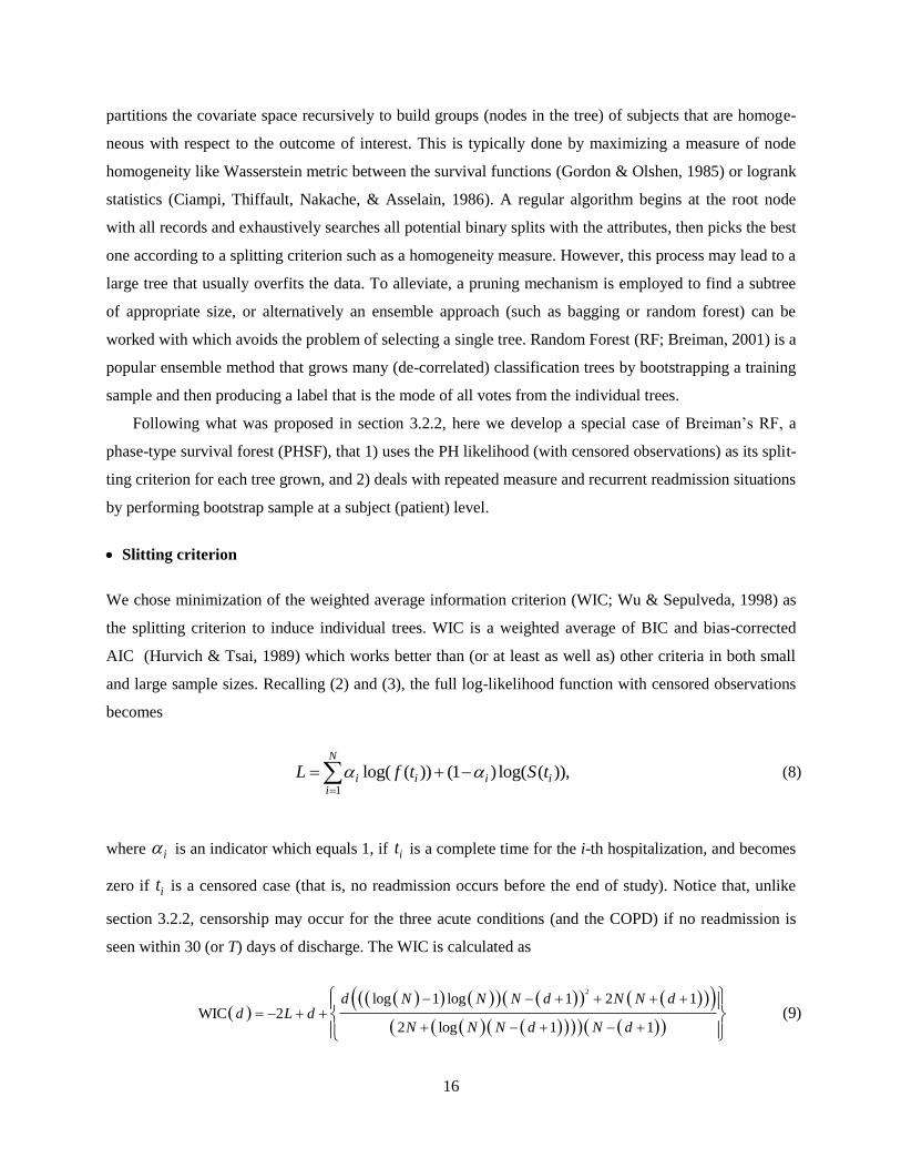
and large sample sizes. Recalling (2) and (3), the full log-likelihood function with censored observations

becomes

1

log( ( )) (1 ) log( ( )),N

i i i ii

L f t S t

(8)

where i is an indicator which equals 1, if it is a complete time for the i-th hospitalization, and becomes

zero if it is a censored case (that is, no readmission occurs before the end of study). Notice that, unlike

section 3.2.2, censorship may occur for the three acute conditions (and the COPD) if no readmission is

seen within 30 (or T) days of discharge. The WIC is calculated as

2

log 1 log 1 2 1WIC 2

2 log 1 1

d N N N d N N dd L d

N N N d N d

(9)

17

in which 2( ) 1d m r , is the PH number of degrees of freedom, and N is the total number of sam-

pled records.

In such a manner, at each node of a tree, if covariate has G values and breaks the node into parti-

tion set 1 2( , , ),G then the total WIC for the split can be expressed by the sum of singular WICs of

every sub-group partitioned by the covariate:

full full1

WIC WIC .( ) ( )g g

G

g

dd

(10)

Therefore, the information gain is defined as the improvement made in the WIC after splitting the node:

full fullWIC WIC ,R RIG d d (11)

where R stands for the node before partition (i.e., the parent node). Beginning from the root node, at eve-

ry single node, we apply one covariate at a time and record the gain for partitioning by that covariate.

Then, we repeat this with other attributes and select a split that minimizes the WIC the most (or yields the

largest gain) to recursively partition into child nodes. Also, if no positive gain can be obtained at a node

by any possible split, the node becomes a terminal node.

Forest development

As mentioned before, since patients (can) have multiple records in the dataset, repeated measures and re-

current events are likely. In this case, the bootstrapped samples are dependent and chances of having cor-

related observations in the in-bag training set are high. Consequently, trees grown may be correlated and

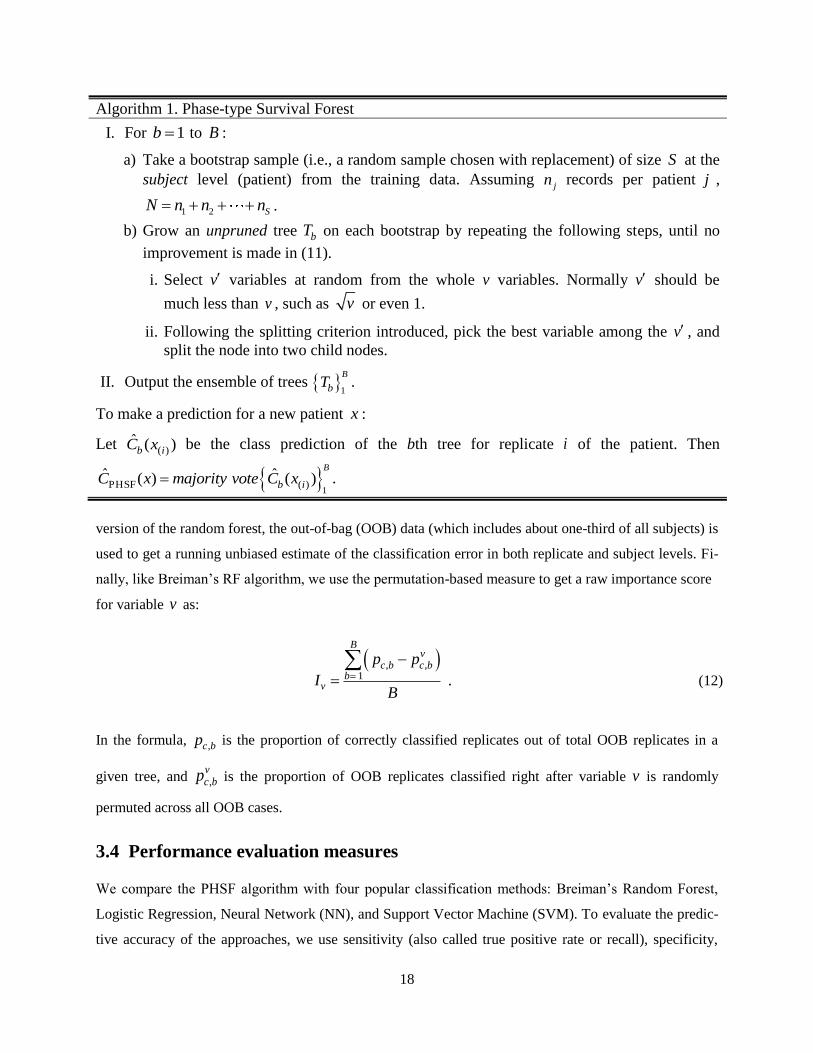
overfitting is plausible. To alleviate this problem, we developed the PHSF algorithm (Algorithm 1) that

performs subject-specific bootstrapping rather than using traditional replicate-based bootstrap. According

to the algorithm, a subject classification is calculated as the label with the maximum number of votes cast

across all records for that subject among all trees. The PHSF is able to produce predictions for specific

replicates of a subject, and it can also be reduced to the original random forest if no replicate per subject

is available. Consistent with the rule-of-thumb, subject-level bootstrapping performed in the algorithm

ensures that about 63% of the subjects (rather than replicates) are elected in-bag. In this way subjects with

more replicates cannot dominate the training process.

Considering that the PHSF generates proportions of votes for each class, similar to data models, we

can have an (unbiased) estimate of the probability that a patient is readmitted. Further, like the original

18

version of the random forest, the out-of-bag (OOB) data (which includes about one-third of all subjects) is

used to get a running unbiased estimate of the classification error in both replicate and subject levels. Fi-

nally, like Breiman’s RF algorithm, we use the permutation-based measure to get a raw importance score

for variable v as:

, ,1 .

Bv

c b c bb

v

p p

IB

(12)

In the formula, ,c bp is the proportion of correctly classified replicates out of total OOB replicates in a

given tree, and ,vc bp is the proportion of OOB replicates classified right after variable v is randomly

permuted across all OOB cases.

3.4 Performance evaluation measures

We compare the PHSF algorithm with four popular classification methods: Breiman’s Random Forest,

Logistic Regression, Neural Network (NN), and Support Vector Machine (SVM). To evaluate the predic-

tive accuracy of the approaches, we use sensitivity (also called true positive rate or recall), specificity,

Algorithm 1. Phase-type Survival Forest

I. For 1b to B :

a) Take a bootstrap sample (i.e., a random sample chosen with replacement) of size S at the

subject level (patient) from the training data. Assuming jn records per patient j ,

1 2 SN n n n .

b) Grow an unpruned tree bT on each bootstrap by repeating the following steps, until no

improvement is made in (11).

i. Select v variables at random from the whole v variables. Normally v should be

much less than v , such as v or even 1.

ii. Following the splitting criterion introduced, pick the best variable among the v , and

split the node into two child nodes.

II. Output the ensemble of trees 1

B

bT .

To make a prediction for a new patient x :

Let ( )ˆ ( )b iC x be the class prediction of the bth tree for replicate i of the patient. Then

1PHSF ( )

ˆ ˆ( ) ( )B

b iC x majority vote C x .

19

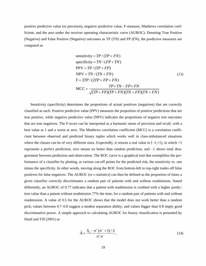
positive predictive value (or precision), negative predictive value, F-measure, Matthews correlation coef-

ficient, and the area under the receiver operating characteristic curve (AUROC). Denoting True Positive

(Negative) and False Positive (Negative) outcomes as TP (TN) and FP (FN), the predictive measures are

computed as

sensitivity / ( )

specificity / ( )

PPV / ( )

NPV / ( )

F 2 / (2 )

MCC( )( )( )( )

TN FP TN

TP TP FP

TN TN FN

TP TP FP FN

TP TN F

TP TP F

P FN

TP FP TP FN TN FP T

N

N FN

(13)

Sensitivity (specificity) determines the proportions of actual positives (negatives) that are correctly

classified as such. Positive predictive value (PPV) measures the proportion of positive predictions that are

true positive, while negative predictive value (NPV) indicates the proportions of negative test outcomes

that are true negatives. The F-score can be interpreted as a harmonic mean of precision and recall, with a

best value at 1 and a worst at zero. The Matthews correlation coefficient (MCC) is a correlation coeffi-

cient between observed and predicted binary tuples which works well in class-imbalanced situations

where the classes can be of very different sizes. Expectedly, it returns a real value in [–1,+1], in which +1

represents a perfect prediction, zero means no better than random prediction, and –1 shows total disa-

greement between prediction and observation. The ROC curve is a graphical tool that exemplifies the per-

formance of a classifier by plotting, at various cut-off points for the predicted risk, the sensitivity vs. one

minus the specificity. In other words, moving along the ROC from bottom-left to top-right trades off false

positives for false negatives. The AUROC (or c-statistics) can then be defined as the proportion of times a

given classifier correctly discriminates a random pair of patients with and without readmission. Stated

differently, an AUROC of 0.77 indicates that a patient with readmission is credited with a higher predic-

tion value than a patient without readmission 77% the time, for a random pair of patients with and without

readmission. A value of 0.5 for the AUROC shows that the model does not work better than a random

pick; values between 0.7–0.8 suggest a modest separation ability; and values bigger than 0.8 imply good

discriminative power. A simple approach to calculating AUROC for binary classification is presented by

Hand and Till (2001) as

0 ( 1) / 2ˆ ,S n n

An n

(14)

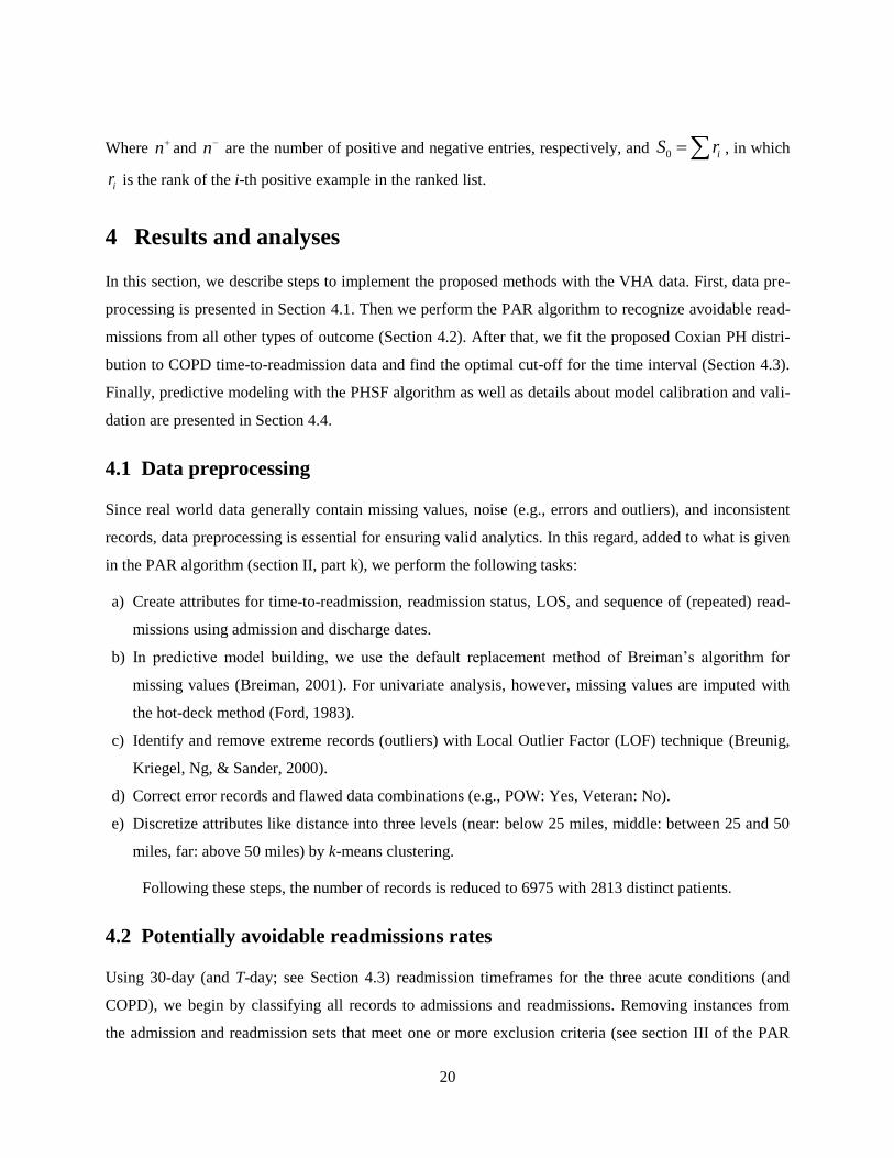
20

Where nand n

are the number of positive and negative entries, respectively, and 0 iS r , in which

ir is the rank of the i-th positive example in the ranked list.

4 Results and analyses

In this section, we describe steps to implement the proposed methods with the VHA data. First, data pre-

processing is presented in Section 4.1. Then we perform the PAR algorithm to recognize avoidable read-

missions from all other types of outcome (Section 4.2). After that, we fit the proposed Coxian PH distri-

bution to COPD time-to-readmission data and find the optimal cut-off for the time interval (Section 4.3).

Finally, predictive modeling with the PHSF algorithm as well as details about model calibration and vali-

dation are presented in Section 4.4.

4.1 Data preprocessing

Since real world data generally contain missing values, noise (e.g., errors and outliers), and inconsistent

records, data preprocessing is essential for ensuring valid analytics. In this regard, added to what is given

in the PAR algorithm (section II, part k), we perform the following tasks:

a) Create attributes for time-to-readmission, readmission status, LOS, and sequence of (repeated) read-

missions using admission and discharge dates.

b) In predictive model building, we use the default replacement method of Breiman’s algorithm for

missing values (Breiman, 2001). For univariate analysis, however, missing values are imputed with

the hot-deck method (Ford, 1983).

c) Identify and remove extreme records (outliers) with Local Outlier Factor (LOF) technique (Breunig,

Kriegel, Ng, & Sander, 2000).

d) Correct error records and flawed data combinations (e.g., POW: Yes, Veteran: No).

e) Discretize attributes like distance into three levels (near: below 25 miles, middle: between 25 and 50

miles, far: above 50 miles) by k-means clustering.

Following these steps, the number of records is reduced to 6975 with 2813 distinct patients.

4.2 Potentially avoidable readmissions rates

Using 30-day (and T-day; see Section 4.3) readmission timeframes for the three acute conditions (and

COPD), we begin by classifying all records to admissions and readmissions. Removing instances from

the admission and readmission sets that meet one or more exclusion criteria (see section III of the PAR

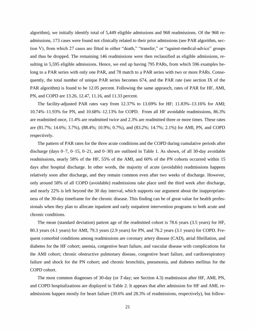
21

algorithm), we initially identify total of 5,449 eligible admissions and 968 readmissions. Of the 968 re-

admissions, 173 cases were found not clinically related to their prior admissions (see PAR algorithm, sec-

tion V), from which 27 cases are fitted in either “death,” “transfer,” or “against-medical-advice” groups

and thus be dropped. The remaining 146 readmissions were then reclassified as eligible admissions, re-

sulting in 5,595 eligible admissions. Hence, we end up having 795 PARs, from which 596 examples be-

long to a PAR series with only one PAR, and 78 match to a PAR series with two or more PARs. Conse-

quently, the total number of unique PAR series becomes 674, and the PAR rate (see section IX of the

PAR algorithm) is found to be 12.05 percent. Following the same appraoch, rates of PAR for HF, AMI,

PN, and COPD are 13.26, 12.47, 11.16, and 11.33 percent.

The facility-adjusted PAR rates vary from 12.37% to 13.69% for HF; 11.83%–13.16% for AMI;

10.74%–11.93% for PN, and 10.68%–12.13% for COPD. From all HF avoidable readmissions, 86.3%

are readmitted once, 11.4% are readmitted twice and 2.3% are readmitted three or more times. These rates

are (81.7%; 14.6%; 3.7%), (88.4%; 10.9%; 0.7%), and (83.2%; 14.7%; 2.1%) for AMI, PN, and COPD

respectively.

The pattern of PAR rates for the three acute conditions and the COPD during cumulative periods after

discharge (days 0–7, 0–15, 0–21, and 0–30) are outlined in Table 1. As shown, of all 30-day avoidable

readmissions, nearly 58% of the HF, 55% of the AMI, and 60% of the PN cohorts occurred within 15

days after hospital discharge. In other words, the majority of acute (avoidable) readmissions happens

relatively soon after discharge, and they remain common even after two weeks of discharge. However,

only around 58% of all COPD (avoidable) readmissions take place until the third week after discharge,

and nearly 22% is left beyond the 30 day interval, which supports our argument about the inappropriate-

ness of the 30-day timeframe for the chronic disease. This finding can be of great value for health profes-

sionals when they plan to allocate inpatient and early outpatient intervention programs to both acute and

chronic conditions.

The mean (standard deviation) patient age of the readmitted cohort is 78.6 years (3.5 years) for HF,

80.3 years (4.1 years) for AMI, 79.3 years (2.9 years) for PN, and 76.2 years (3.1 years) for COPD. Fre-

quent comorbid conditions among readmissions are coronary artery disease (CAD), atrial fibrillation, and

diabetes for the HF cohort; anemia, congestive heart failure, and vascular disease with complications for

the AMI cohort; chronic obstructive pulmonary disease, congestive heart failure, and cardiorespiratory

failure and shock for the PN cohort; and chronic bronchitis, pneumonia, and diabetes mellitus for the

COPD cohort.

The most common diagnoses of 30-day (or T-day; see Section 4.3) readmission after HF, AMI, PN,

and COPD hospitalizations are displayed in Table 2. It appears that after admission for HF and AMI, re-

admissions happen mostly for heart failure (39.6% and 28.3% of readmissions, respectively), but follow-

22

ing hospitalizations for PN and COPD, patients get readmitted because of COPD (21.4% and 32.5%, in

turn). Also, the top five readmission diagnoses contribute to 63.2% of all readmissions after HF, 59.4% of

all readmissions after AMI, 55.6% of all readmissions after PN, and 65.1% of all readmissions after

COPD.

Further, we realized that the most frequent reasons for avoidable readmissions in all conditions are re-

lated to “recurrence or extension of the reason (Section V, part b)” and “medical complications (Section

V, part d)”, with an average of 54.7% and 23.2% through all the hospitals. As expected, in none of the

acute and chronic conditions is the proportion of non-clinically related readmissions over 15.4 percent.

Next, we compared percentages of readmissions calculated by our method (PAR) to those of the 3M

method for the three acute conditions in the four hospitals (Figure 3). In our method, consistent with the

literature (Medicare Payment Advisory Commission, 2007), we observe that a greater proportion of all

readmissions can be avoided in the first two weeks after discharge, but the contribution declines as time

passes. Compared to the 3M approach, our method considers (slightly) fewer rehospitalizations as being

avoidable and produces lower rates of readmission throughout all periods after discharge. A probable rea-

son for this may be related to the CMS- and VHA-specific exclusions of our method, which is not found

in the 3M approach. Besides, almost the same trend (not shown here) is seen for the COPD readmissions

but over an extended time interval following discharge.

4.3 Optimal COPD readmission timeframe

In this section, we fit the proposed Coxian PH distribution to COPD time-to-readmission data in order to

find the optimal cut-off point that defines avoidable readmissions. Using empirical data, we first examine

the percentile distribution of times in Table 3.

As shown, the median time-to-(avoidable) readmission is about 36 days and the distribution is (highly)

right skewed, with more than half of patients readmitted after the 30th day from discharge. This implies

that, unlike acute conditions, poor quality of inpatient care for chronic conditions may reveal itself after

30 days from discharge. So setting the 30-day as a fixed timeframe for both acute and chronic conditions

may not be appropriate.

We then applied the EMpht software to estimate the phase-type generator Q in (5) using COPD

time-to-readmission data from FY 11–12. In brief, the program starts with an initial guess (0)

Q (for the

non-zero elements in (5)) and proceeds with a number of iterations of the EM algorithm to increase the

log-likelihood function 1

log exp( )( )N

i

t

π Q Q1 . Fixing the maximum number of iterations at 5000

23

runs and Runge-Kutta step length at

0.1

max i iQ (in which

max i iQ is the largest absolute value of the

diagonal element of the last estimate of Q ), we configure different Coxian PH structures by modifying

the order of the sub-class Markov processes (i.e., parameters m and r ). This way, we start with 1m ,

examine various levels of r from 1 to 10, and pick the best in terms of AIC and BIC; then we repeat this

for 2m until 10m . We stop the search if the log-likelihood does not improve in any intermediate

level. Also due to non-identifiability of the parametrization of the phase-type distribution (O’Cinneide,

1990), we do several fits starting with various initial values produced in previous runs. The results of best

fits at each level of m are then summarized in Table 4.

It is apparent that there is no improvement in the fits after the fourth phase of the Short-Stay group

(i.e., m=4). Hence an order 6 of the Coxian PH distribution with 4 and 6 phases for the Short-Stay and

Long-Stay groups respectively is considered to most suitably represent the time-to-readmission process of

the COPD patients in the dataset. Note that we do not show fits after (m=5) as they provide no further

enhancements.

The estimates of the intensity rates in (5) along with their standard errors are calculated in Table 5.

Given the small amounts of error, we see that the parameters are well estimated with EMpht. Also note

that 1 , 2 , and 3 belong to the Short-Stay group, while 4 and 5 are related to the Long-Stay

group. According to the table, the probability of a patient being in the Short-Stay group is calculated as

1.260.4437

1.26 1.58p

, which means that the COPD patients spend about 44.37% of their time in the

Short-Stay group in the community before returning to the hospital.

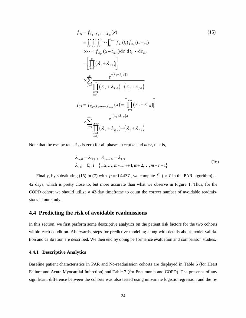
Then, in order to solve (7) and obtain the optimal COPD readmission timeframe, we need to derive

the PDFs SSf and LSf . This can be done based on a convolution of a set of independent exponential

variables ( iX ) as follows (Ross, 2009):

24

1 2

1 2 1

1 2

0

SS

1 2 10 0 0 0

1 1 2 1

1

0

( ) (15)

( ) ( )

( )d d d

m

j j

m

m m

i

m

m

i i

k

X X X

x t t t

X X

X

x

f f x

f t f t t

f x t t t t

e

1 2

0

1

1

LS

1

1

1

0 0

0

0 0

( )

j j

m r

m

mj

kk j

m r

m rj

kk j

im r

k j j

i i

k k j j

X X X

x

f f x

e

Note that the escape rate 0i is zero for all phases except m and m+r, that is,

0 SS 0 L S

0 1, 2, , -1, 1, m 2, , 1

,

0;

m

i

m r

m m m ri

(16)

Finally, by substituting (15) in (7) with 0.4437p , we compute t (or T in the PAR algorithm) as

42 days, which is pretty close to, but more accurate than what we observe in Figure 1. Thus, for the

COPD cohort we should utilize a 42-day timeframe to count the correct number of avoidable readmis-

sions in our study.

4.4 Predicting the risk of avoidable readmissions

In this section, we first perform some descriptive analytics on the patient risk factors for the two cohorts

within each condition. Afterwards, steps for predictive modeling along with details about model valida-

tion and calibration are described. We then end by doing performance evaluation and comparison studies.

4.4.1 Descriptive Analytics

Baseline patient characteristics in PAR and No-readmission cohorts are displayed in Table 6 (for Heart

Failure and Acute Myocardial Infarction) and Table 7 (for Pneumonia and COPD). The presence of any

significant difference between the cohorts was also tested using univariate logistic regression and the re-

25

sults are shown in terms of P-Values [missing values are imputed by the hot-deck method (Ford, 1983)].

Since the same patient could have several avoidable readmissions during the study period, we used gener-

alized estimation equation to adjust for serial correlations among readmissions of the same patient.

During the study, a total of 5,595 eligible admissions were made in the four VA hospitals, out of

which about 14. 21% were followed by an unnecessary rehospitalization. Note that this rate is different

from what is reported in Section 4.2 (which is 12.05%) because here we count each readmission

separately rather than as members of a PAR series. In all conditions, the populations are generally male

(>86%), married (>51%), older (>67 years), and live within 25 miles of a VA facility (>60%). More than

21% in all conditions do not have private insurance or insurance through Medicare or Medicaid programs.

More than half of patients in all conditions are admitted directly from their home and more than 50% have

one to four past-year hospitalizations. On average, the care assessment score is higher in respiratory

diseases (near 69) compared to circulatory conditions (about 66). Almost 18% of the patients are also

diagnosed with more than ten HCCs (not shown in the tables). Note that in the attribute “source of

admission,” class ‘transfer’ is related to those patients who are transferred only among the four VA

hospitals, and ‘Other’ is related to some other admission sources such as observation/examination,

non-VA hospitals not under VA auspices, community nursing homes under (or not under) VA auspices,

non-veteran hospitals, etc. Further, priority groups 1, 2, and 3 are generally assigned to veterans with

service-connected disabilities of > 50%, [30%, 50%), and [20%, 30%), respectively. Other groups are as

follows: 4, catastrophically disabled veterans; 5, low income or Medicaid; 6, Agent Orange or Gulf War

veterans; 7, non-service connected with income being below HUD; and 8, non-service connected with

income being above HUD. For each condition, patient comorbidities are identified with the help of

Comorbidity Software (Kaboli et al., 2012), using ICD-9-CM and DRG codes from the index

hospitalization and any admission in the 12 months prior.

It is observed that patients who are subsequently readmitted are elderly and usually have a greater

number of comorbidities. Male patients have on average a greater chance to be readmitted in HF and

COPD cohorts rather than females, but this cannot be generalized since the VA sample here contains only

about 8% female patients. The analysis shows that length of stay is not generally associated with odds of

avoidable readmission, when patient and facility characteristics are not controlled for. However, after ad-

justing for the case-mix and service-mix (not shown here), the relation tends to be negative (about 7.3%

increase for each in-hospital day lower than expected), which implies that shorter individual LOS is gen-

erally connected with higher risk of readmission. Therefore, consistent with (Kaboli et al., 2012), we ob-

serve that significant reduction in LOS, without simultaneously improving inpatient care, is more likely to

result in premature discharge and rehospitalization. Further, enrollment priority turns out to be highly

linked with odds of readmission in all conditions, especially when it comes to catastrophically disabled

26

veterans (increases of .2% in AMI to 10.9% in HF). Furthermore, the odds of avoidable readmissions are

significantly higher in patients exposed to ionizing radiation and Agent Orange in all conditions. Among

the comorbid conditions, having diabetes and cancer increases the chance of readmission, as does having

mental disorders and substance abuse (with harsher effect in circulatory conditions).

4.4.2 Predictive modeling with PHSF

Following Algorithm 1, we used the entire set of patient risk factors to develop a readmission prediction

model. Additionally, we create two more covariates, namely, “sequence” (see Section 4.1) and “Charlson

comorbidity index” (Charlson et al., 1987) and entered them into the analysis. For non-categorical varia-

bles in the candidate set (i.e., age, LOS, CAN score, sequence, and Charlson index), we evaluated differ-

ent cut-off points to split the dataset into binary partitions and explore the optimal cutpoint that most dis-

criminates high vs. low risk using operating characteristic curves (with whole dataset). We then used this

ROC-generated cutpoint for further analyses. Also for categorical features with more than two classes

(like race), following Friedman, Hastie, and Tibshirani (2009), we optimally select a series of binary

splits (instead of multiway splits) that produce the best discrimination results.

We begin with the baseline model that uses all sampled data points (5,595 records) in the sub-

ject-specific bootstrapped PHSF and we let the forest internally perform cross-validation using OOB

samples during each run. The number of trees and the number of variables to try at each split are set to

6,000 and 5, respectively. Also we set the cutpoints with respect to minimizing the WIC criterion (see

Section 3.1.1) as follows: Age, 68 (years); LOS, 5 (days); CAN score, 66; sequence, 3; and Charlson in-

dex, 4.5. Results of variable importance are summarized in Table 8 (Sig. stands for significance level). As

illustrated, almost all statistically significant variables (Sig. <.05) refer to overall health and agedness fac-

tors, which may reflect a generalized vulnerability to disease among recently discharged patients—

inpatients regularly lose their strength and develop new difficulties in doing their day-to-day activities

(Gill, Allore, Gahbauer, & Murphy, 2010). Interestingly, ‘sequence’ turns out to be (positively) related to

readmission risk, which highlights the fact that the chance of unnecessary returns to hospital is greater in

patients with prior history of readmission.

In the baseline model, the c-statistics is .793; sample-level OOB error rates are 3.16%, 2.35%, and

8.05% for overall, No-readmission class, and PAR class, respectively; and there are large interactions

[based on Breiman’s variable interaction model (Breiman, 2001)] between Agent Orange and Radiation,

between Priority and LOS, and between Priority and Insurance, to name a few.

27

Model calibration

We then calibrated the baseline model as follows: 1) we focused only on the 16 most important variables

found in the baseline model; 2) we imputed missing values based on Breiman’s replacement technique

(Breiman, 2001); 3) we modified the optimal cut-off points with regards to maximizing the c-statistics

(the new cutpoints are 69 years for age, 70 for CAN score, and 4.7 for Charlson index, while others re-

main unchanged); and 4) we altered the class weights to 1 on class ‘No-readmission’ and 8 on class

‘PAR’, to adjust for the imbalanced prediction errors in the classes. Then we rerun the model with 10,000

trees and 4 variables to try at each split. Depiction of variable importance for the calibrated model is

shown in Table 9. Expectedly, the ranking of variables does not change but we achieved better results in

terms of scores and significance levels. It is noticed that, though Mental disorder and Malignant neoplasm

are only marginally significant, we decide to keep them in the final model since 1) they are both medical-

ly significant in contribution to the risk of readmission, and 2) they together contribute largely to the

model discrimination ability.

In the calibrated model, the c-statistics jumps to .836; no serious interactions remain among variables;

and the overall, No-readmission, and PAR error rates become 3.67%, 2.51%, and 2.64%, respectively. It

is remarkable that the calibrated model considerably decreases PAR misclassification rate, but at the ex-

pense of increasing the overall error rate a little bit. We perceive that this tuning in class weights is really

appealing for our situation because in readmission prediction models, the cost of false negatives (which

correspond to readmitted patients incorrectly predicted as No-readmission) is usually much higher than

the cost of false positives (which correspond to non-readmitted patients incorrectly predicted as PAR cas-

es).

Since the PHSF method takes an ensemble approach of trees, as we mentioned earlier, we can obtain

an unbiased estimate of PAR probability for each patient. Therefore, it is possible to further check the

model calibration by evaluating predicted and actual PAR rates at different risk deciles. These results ap-

pear in Table 10 and Figure 4.

We note that, both on average and over the whole range of predictions, the predicted probability of

readmission matches up well with the actual probabilities. Average predicted readmission (not shown

here) also monotonically increases with growing risk, ranging from 8.79% in the lowest decile to 43.75%

in the highest, a range of 34.96% in total. For the 12% of readmissions that happens between deciles four

and five, the PHSF model under-predicts by roughly 8.5%. It also over-predicts by about 4%–14% for the

small number of readmissions (21%) which occur in deciles 6–10.

28

Model validation

Here, we used the calibrated model and studied its internal validity (also called reproducibility), based on

the same population underlying the sample. To this end, since the PHSF does perform bootstrapping in-

ternally, we slightly modified the split-sample technique for our purposes: we randomly partitioned the

sample into 50% training and 50% testing sets and redid this 7 times. For each partition we ran the PHRF

algorithm and obtained the c-statistics. The average c-statistics for the seven runs of training sets

reached .839 and for the test sets, it was .821. Hence, there exists an “optimism” of .018 in the mean AU-

ROCs for the training and testing splits, and as a result, the internally-validated (or optimism-corrected)

c-statistics is estimated as .818.

To provide more robust evidence of validity, we further conducted external (in fact: spatial)

validation (also called generalizability) with a new sample of 478 patients admitted (with primary

diagnosis of HF, AMI, PN, and COPD) in the months of August and September 2012. It is noted that we

included the same patient factors studied in the new sample. The c-statistics in the external sample

decreased to .809 (a decrease of .027) which is slightly more than results from internal validation (a

decrease of .018). However, both internal and external validations confirm the superiority of our proposal

over the current approaches in terms of discrimination power and stability. Nonetheless, we obtain greater

c-statistics (at least .813) when the PHSF is applied separately on each condition. It should also be

remarked that with the current sample data, the CMS endorsed model can only produce a c-statistics of

about .63.

4.4.3 Numerical comparisons

In this section, we evaluate the proposed PHSF method with Logistic Regression (LR), Breiman’s Radom

Forest (RF), Support Vector Machine (SVM), and Neural Network (NN) in terms of predictive measures

introduced in Section 3.4 (plus mean squared error). The models are built and compared with the R ver-

sion 3.0.2 (RDC Team, 2005) using packages randomForest (Liaw & Wiener, 2002), e1071

(Dimitriadou, Hornik, Leisch, Meyer, & Weingessel, 2008), glm2 (Marschner, 2011), and also MATLAB

neural network toolbox (Demuth & Beale, 1993). It is worth mentioning that we used different kernels

such as polynomial and radial basis function for the SVM method; and for the NN approach, we also test-

ed for two and three layers with different numbers of sigmoid hidden neurons and linear output neurons.

For the pure random forest method, we did the same calibration as with the PHSF, and for the logistic

regression, we used generalized estimation equation to account for clustering at the patient level. The

comparison results are summarized in Table 11 and Figure 5. As shown, the proposal works better than

29

other alternatives in all predictive criteria. The Breiman’s random forest approach and SVM produce very

close results in this sample but the NN approach seems unable to compete with other models having a

modest discrimination of about 0.7. Not surprisingly, all models predict ‘No-readmission’ cases better

than the PAR cases. It is of interest that SVM slightly outperforms the RF in terms of precision (.5%

higher) and true negative rate (.17% higher). Furthermore, in the overall spectrum of false positive rates,

the proposal assigns a higher probability of readmission for a patient with PAR compared to a ‘No-

readmission’ patient, about 83.6% of the times. Looking at different ROC stairs graphs, we can infer that,

with a false positive rate between .09 to .25, our PHSF is placed higher than others, but it falls behind the

SVM and NN in case of very small rates of false positive. In higher false positive rates, we observe that

RF and SVM are very similar in discrimination ability and they work as well as PHSF beyond .7 false

positive rate. However, logistic regression turns out to fall short at a type I error rate of .8 to .9.

5 Conclusion

Concentration on reducing unnecessary readmission has never been higher, especially with the CMS

augmenting the rates of penalties and introducing new waves of diseases that will be under scrutiny dur-

ing next years. In response to this policy shift, hospitals and clinicians are become more interested in ana-

lytics ways to identify patients at elevated risk of avoidable readmission, since such tools can ultimately

be used to guide more appropriate discharge planning and efficient resource utilization. Although a varie-

ty of approaches have been proposed to identify patients with higher risk, their potentials have been lim-

ited mainly because they do not incorporate timing of readmission in their prediction and/or they are not

accurate enough (Kansagara et al., 2011).

In this study, we make several contributions to readmission reduction studies. First, we address the

problem of characterizing avoidable (or unnecessary) readmissions from all other types of outcomes. Our

algorithm (PAR) is based on administrative data and takes a more accurate look at preventability compo-

nents of rehospitalization compared to existing methods. We also suggest using a more comprehensive

risk adjustment tool (DCG/HCC) in counting avoidable readmissions, as well as getting help from other

sources of information, like clinic visits between index admission and readmission, in assessing the

avoidability of readmissions.

Second, we assert that the government-endorsed 30-day timeframe that is used to count readmissions

is not “optimal” for chronic conditions such as COPD. Therefore, we develop a stochastic model based on

Coxian phase-type distribution to analytically calculate the optimum cut-point that best stratifies among

quickly-readmitted and slowly-readmitted COPD patients. We then adopt the new time window in the

PAR algorithm to adjust for COPD readmissions.

30

Third, by combining algorithmic and data models, we put forward a hybrid predictive approach that

exploits good aspects of classification and timing-based analytics models. We then demonstrate the supe-

riority of our model over current solutions with respect to various accuracy criteria. Further, to confirm

that the high discrimination ability of our proposal is irrespective to overfitting, we perform internal and

external validation practices. Also, unlike some studies in the literature, we do not limit our work to a

specific disease (Hernandez et al., 2010) or within a specific hospital (Smith, Huster, Fitzgerald, & Martin,

1996), but instead we aggregate data from four different VA facilities containing inpatients diagnosed

with four different conditions.

Even though our results introduce new aspects of readmission studies, one should pay attention to

some limitations in interpreting and generalizing them. First, the data used in the study is from one region

(Veteran Integrated Service Network 11, Veterans In Partnership) in the State of Michigan, with a veteran

population that is mostly male and veteran, and a government-funded care delivery system; hence the re-

sults may not be identical in other health care systems. Second, the study is limited to administrative data

(that are regularly available to all health plans) and it does not have laboratory test results and vital signs

such as hemoglobin or serum level at discharge, which may affect the risk of unnecessary readmission.

In future work, we plan to use our proposal to compare and profile the hospitals on their readmission

rates using proper risk adjustment for case mix and service mix. The approach currently employed by the

CMS (and the VHA) is to calculate a ratio of observed to expected outcomes for a given hospital, and

evaluate it across the normal range of all other hospitals given the same mix. Methods in this context are

primarily based on models in which the hospital effects on outcome are taken as random. Nonetheless,

they have been recently argued because 1) they often produce biased estimates of outcomes at the

provider level; and 2) they cannot prevent confounding issues when the patient characteristics are

correlated with facility effects (Kalbfleisch & Wolfe, 2013).

References

Akaike, H. (1974). A new look at the statistical model identification. Automatic Control, IEEE

Transactions on, 19(6), 716-723.

Alaeddini, A., Yang, K., Reddy, C., & Yu, S. (2011). A probabilistic model for predicting the probability

of no-show in hospital appointments. Health Care Manag Sci, 14(2), 146-157.

Asmussen, S. EMpht software Retrieved November 14, 2013, from

http://home.imf.au.dk/asmus/pspapers.html

Asmussen, S., Nerman, O., & Olsson, M. (1996). Fitting phase-type distributions via the EM algorithm.

Scandinavian Journal of Statistics, 419-441.

Au, A. G., McAlister, F. A., Bakal, J. A., Ezekowitz, J., Kaul, P., & van Walraven, C. (2012). Predicting

the risk of unplanned readmission or death within 30 days of discharge after a heart failure

hospitalization. Am Heart J, 164(3), 365-372.

31

Bayerstadler, A., Benstetter, F., Heumann, C., & Winter, F. (2013). A predictive modeling approach to

increasing the economic effectiveness of disease management programs. Health Care Manag Sci,

1-18.

Benbassat, J., & Taragin, M. (2000). Hospital readmissions as a measure of quality of health care:

advantages and limitations. Archives of Internal Medicine, 160(8), 1074-1081.

Berry, J. G., Toomey, S. L., Zaslavsky, A. M., Jha, A. K., Nakamura, M. M., Klein, D. J., . . . Schuster, M.

A. (2013). Pediatric readmission prevalence and variability across hospitals. Journal of the

American Medical Association, 309(4), 372-380.

Breiman, L. (1993). Classification and regression trees: CRC press.

Breiman, L. (2001). Random forests. Machine learning, 45(1), 5-32.

Breunig, M. M., Kriegel, H.-P., Ng, R. T., & Sander, J. (2000). LOF: identifying density-based local

outliers. Paper presented at the ACM Sigmod Record.

Charlson, M. E., Pompei, P., Ales, K. L., & MacKenzie, C. R. (1987). A new method of classifying

prognostic comorbidity in longitudinal studies: development and validation. Journal of chronic

diseases, 40(5), 373-383.

Chassin, M. R., Loeb, J. M., Schmaltz, S. P., & Wachter, R. M. (2010). Accountability measures—using

measurement to promote quality improvement. New England Journal of Medicine, 363(7), 683-688.

Ciampi, A., Thiffault, J., Nakache, J.-P., & Asselain, B. (1986). Stratification by stepwise regression,

correspondence analysis and recursive partition: a comparison of three methods of analysis for

survival data with covariates. Computational statistics & data analysis, 4(3), 185-204.

Davis, R. B., & Anderson, J. R. (1989). Exponential survival trees. Statistics in Medicine, 8(8), 947-961.

Demuth, H., & Beale, M. (1993). Neural network toolbox for use with MATLAB.

Dimitriadou, E., Hornik, K., Leisch, F., Meyer, D., & Weingessel, A. (2008). Misc functions of the

Department of Statistics (e1071), TU Wien. R package, 1.5-24.

Fackrell, M. (2009). Modelling healthcare systems with phase-type distributions. Health Care Manag Sci,

12(1), 11-26.

Fetter, R. B., Shin, Y., Freeman, J. L., Averill, R. F., & Thompson, J. D. (1980). Case mix definition by

diagnosis-related groups. Med Care, 18(2), 1-53.

Ford, B. L. (1983). An overview of hot-deck procedures. Incomplete data in sample surveys, 2(Part IV),

185-207.

Friedman, J., Hastie, T., & Tibshirani, R. (2009). The Elements of Statistical Learning: Data Mining,

Inference, and Prediction. Springer Series in Statistics.

Gill, T. M., Allore, H. G., Gahbauer, E. A., & Murphy, T. E. (2010). Change in disability after

hospitalization or restricted activity in older persons. Journal of the American Medical Association,

304(17), 1919-1928.

Goldfield, N. I., McCullough, E. C., Hughes, J. S., Tang, A. M., Eastman, B., Rawlins, L. K., & Averill,

R. F. (2008). Identifying potentially preventable readmissions. Health care financing review, 30(1),

75-91.

Golub, G. H., & Van Loan, C. F. (2012). Matrix computations (Vol. 3): Johns Hopkins University Press.

Gordon, L., & Olshen, R. (1985). Tree-structured survival analysis. Cancer treatment reports, 69(10),

1065.

Halfon, P., Eggli, Y., van Melle, G., Chevalier, J., Wasserfallen, J.-B., & Burnand, B. (2002). Measuring

potentially avoidable hospital readmissions. Journal of clinical epidemiology, 55(6), 573-587.

Hand, D. J., & Till, R. J. (2001). A simple generalisation of the area under the ROC curve for multiple

class classification problems. Machine learning, 45(2), 171-186.

Hansen, L. O., Young, R. S., Hinami, K., Leung, A., & Williams, M. V. (2011). Interventions to reduce

30-day rehospitalization: a systematic review. Annals of Internal Medicine, 155(8), 520-528.

Hasan, M. (2001). Readmission of patients to hospital: still ill defined and poorly understood.

International Journal for Quality in Health Care, 13(3), 177-179.

Hernandez, A. F., Greiner, M. A., Fonarow, G. C., Hammill, B. G., Heidenreich, P. A., Yancy, C. W., . . .

Curtis, L. H. (2010). Relationship between early physician follow-up and 30-day readmission

32

among Medicare beneficiaries hospitalized for heart failure. Journal of the American Medical

Association, 303(17), 1716-1722.

Horwitz, L., Partovian, C., Lin, Z., Herrin, J., Grady, J., Conover, M., . . . Ross, J. (2011). Hospital-wide

(all-condition) 30-day risk-standardized readmission measure. Retrieved Sep 27, 2013, from

http://146.123.140.205/Medicare/Quality-Initiatives-Patient-Assessment-

Instruments/MMS/downloads/MMSHospital-WideAll-ConditionReadmissionRate.pdf

Hurvich, C. M., & Tsai, C.-L. (1989). Regression and time series model selection in small samples.

Biometrika, 76(2), 297-307.

Jencks, S. F., Williams, M. V., & Coleman, E. A. (2009). Rehospitalizations among patients in the

Medicare fee-for-service program. New England Journal of Medicine, 360(14), 1418-1428.

Johnson, M. A. (1993). Selecting parameters of phase distributions: Combining nonlinear programming,

heuristics, and Erlang distributions. ORSA Journal on Computing, 5(1), 69-83.

Joynt, K. E., Orav, E. J., & Jha, A. K. (2011). Thirty-day readmission rates for Medicare beneficiaries by

race and site of care. Journal of the American Medical Association, 305(7), 675-681.

Kaboli, P. J., Go, J. T., Hockenberry, J., Glasgow, J. M., Johnson, S. R., Rosenthal, G. E., . . . Vaughan-

Sarrazin, M. (2012). Associations between reduced hospital length of stay and 30-day readmission

rate and mortality: 14-year experience in 129 Veterans Affairs hospitals. Annals of Internal

Medicine, 157(12), 837-845.

Kalbfleisch, J. D., & Wolfe, R. A. (2013). On monitoring outcomes of medical providers. Statistics in

Biosciences, 1-17.

Kansagara, D., Englander, H., Salanitro, A., Kagen, D., Theobald, C., Freeman, M., & Kripalani, S.

(2011). Risk prediction models for hospital readmission: a systematic review. Journal of the

American Medical Association, 306(15), 1688-1698.

Krumholz, H. M., Wang, Y., Mattera, J. A., Wang, Y., Han, L. F., Ingber, M. J., . . . Normand, S.-L. T.

(2006). An administrative claims model suitable for profiling hospital performance based on 30-

day mortality rates among patients with an acute myocardial infarction. Circulation, 113(13), 1683-

1692.

Liaw, A., & Wiener, M. (2002). Classification and Regression by randomForest. R news, 2(3), 18-22.

Marschner, I. C. (2011). glm2: Fitting Generalized Linear Models with Convergence Problems. The R

Journal, 3(2), 12-15.

McLachlan, G., & Peel, D. (2004). Finite mixture models: Wiley-Interscience.

Medicare Payment Advisory Commission. (2007). Report to the Congress: promoting greater efficiency

in Medicare: Medicare Payment Advisory Commission (MedPAC).

Mull, H. J., Chen, Q., O’Brien, W. J., Shwartz, M., Borzecki, A. M., Hanchate, A., & Rosen, A. K. (2013).

Comparing 2 Methods of Assessing 30-Day Readmissions: What is the Impact on Hospital

Profiling in the Veterans Health Administration? Med Care, 51(7), 589-596.

National Quality Measures Clearinghouse. Ambulatory care sensitive conditions: age-standardized acute

care hospitalization rate for conditions where appropriate ambulatory care prevents or reduces the

need for admission to the hospital, per 100,000 population younger than age 75 years. Retrieved

September 06, 2013, from http://www.qualitymeasures.ahrq.gov/content.aspx?id=35186

O’Cinneide, C. A. (1990). Characterization of phase-type distributions. Stochastic Models, 6(1), 1-57.

Pope, G. C., Kautter, J., Ellis, R. P., Ash, A. S., Ayanian, J. Z., Ingber, M. J., . . . Robst, J. (2004). Risk

adjustment of Medicare capitation payments using the CMS-HCC model. Health care financing

review, 25(4), 119-141.

Pracht, E. E., & Bass, E. (2011). Exploring the Link between Ambulatory Care and Avoidable

Hospitalizations at the Veteran Health Administration. Journal for Healthcare Quality, 33(2), 47-

56.

RDC Team. (2005). R: A language and environment for statistical computing: R Foundation for

Statistical Computing. Vienna, Austria, 2013. http://www.R-project.org.

Reed, R. L., Pearlman, R. A., & Buchner, D. M. (1991). Risk factors for early unplanned hospital

readmission in the elderly. Journal of general internal medicine, 6(3), 223-228.

33

Reinecke, P., Krauß, T., & Wolter, K. (2012). Cluster-based fitting of phase-type distributions to

empirical data. Computers & Mathematics with Applications, 64(12), 3840-3851.

Ross, S. M. (2009). Introduction to probability models (10 ed.): Academic Press.

Sales, A. E., Liu, C.-F., Sloan, K. L., Malkin, J., Fishman, P. A., Rosen, A. K., . . . Perrin, E. (2003).

Predicting costs of care using a pharmacy-based measure risk adjustment in a veteran population.

Med Care, 41(6), 753-760.

Schwarz, G. (1978). Estimating the dimension of a model. The annals of statistics, 6(2), 461-464.

Shams, I., Ajorlou, S., & Yang, K. (2013). A Patient Readmission Risk Prediction Model. Paper presented

at the Proceedings of the 2013 Industrial and Systems Engineering Research Conference.

Shulan, M., Gao, K., & Moore, C. D. (2013). Predicting 30-day all-cause hospital readmissions. Health

Care Manag Science, 16(2), 167-175.

Smith, D. M., Huster, G. A., Fitzgerald, J. F., & Martin, D. K. (1996). Risk factors for nonelective

hospital readmissions. Journal of general internal medicine, 11(12), 762-764.

Stroock, D. W. (2005). An Introduction to Markov Processes. New York: Springer.

Tsai, T. C., Joynt, K. E., Orav, E. J., Gawande, A. A., & Jha, A. K. (2013). Variation in Surgical-

Readmission Rates and Quality of Hospital Care. New England Journal of Medicine, 369(12),

1134-1142.

van Walraven, C., Bennett, C., Jennings, A., Austin, P. C., & Forster, A. J. (2011). Proportion of hospital

readmissions deemed avoidable: a systematic review. Canadian Medical Association Journal,

183(7), E391-E402.

Westert, G. P., Lagoe, R. J., Keskimäki, I., Leyland, A., & Murphy, M. (2002). An international study of

hospital readmissions and related utilization in Europe and the USA. Health Policy, 61(3), 269-278.

Wu, T.-J., & Sepulveda, A. (1998). The weighted average information criterion for order selection in time

series and regression models. Statistics & probability letters, 39(1), 1-10.

Zhang, J., Yoon, S. W., Khasawneh, M. T., Srihari, K., & Poranki, S. (2013). Hospital Readmission

Prediction Using Swarm Intelligence-based Support Vector Machines. Paper presented at the

Proceedings of the 2013 Industrial and Systems Engineering Research Conference.

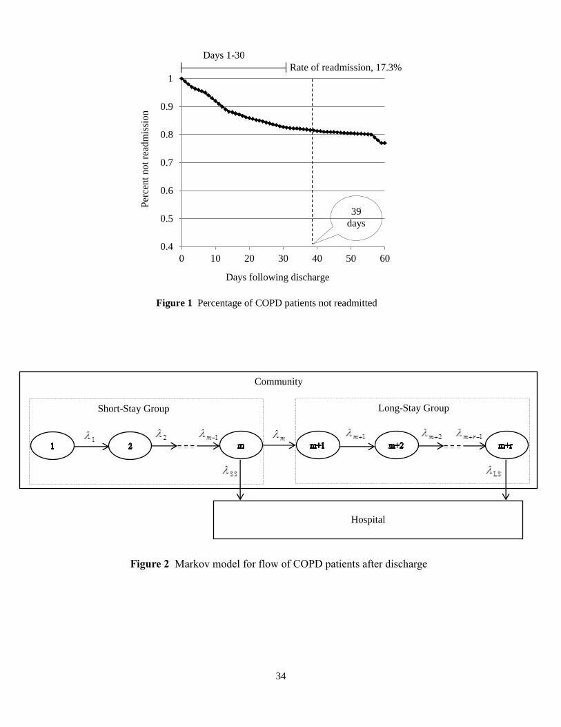
34

Days following discharge

Days 1-30

Rate of readmission, 17.3%

Per

cent

not

read

mis

sion

0.4

0.5

0.6

0.7

0.8

0.9

1

0 10 20 30 40 50 60

39

days

Figure 1 Percentage of COPD patients not readmitted

Figure 2 Markov model for flow of COPD patients after discharge

Community

Hospital

Long-Stay Group Short-Stay Group

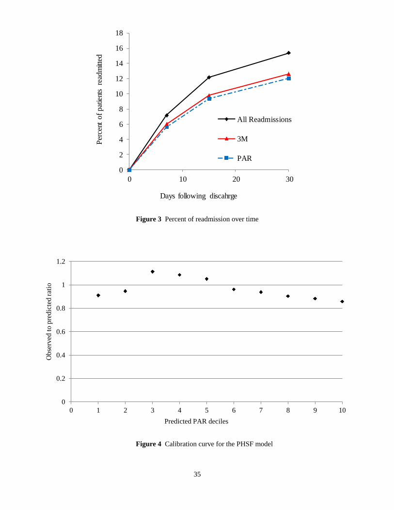
35

Figure 4 Calibration curve for the PHSF model

0

0.2

0.4

0.6

0.8

1

1.2

0 1 2 3 4 5 6 7 8 9 10

Ob

serv

ed t

o p

redic

ted r

atio

Predicted PAR deciles

Figure 3 Percent of readmission over time

0

2

4

6

8

10

12

14

16

18

0 10 20 30

Per

cent

of

pat

ient

s re

adm

itted

Days following discahrge

All Readmissions

3M

PAR

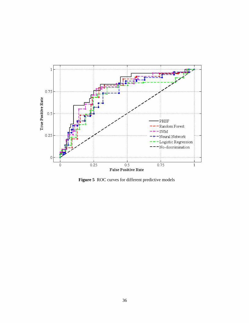
36

Figure 5 ROC curves for different predictive models

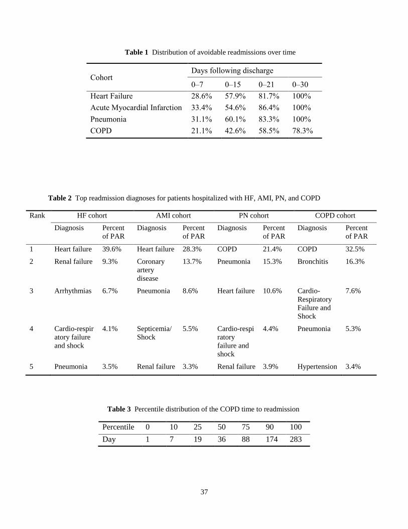
37

Table 1 Distribution of avoidable readmissions over time

Table 2 Top readmission diagnoses for patients hospitalized with HF, AMI, PN, and COPD

Rank HF cohort AMI cohort PN cohort COPD cohort

Diagnosis Percent

of PAR

Diagnosis Percent

of PAR

Diagnosis Percent

of PAR

Diagnosis Percent

of PAR

1 Heart failure 39.6% Heart failure 28.3% COPD 21.4% COPD 32.5%

2 Renal failure 9.3% Coronary

artery

disease

13.7% Pneumonia 15.3% Bronchitis 16.3%

3 Arrhythmias 6.7% Pneumonia 8.6% Heart failure 10.6% Cardio-

Respiratory

Failure and

Shock

7.6%

4 Cardio-respir

atory failure

and shock

4.1% Septicemia/

Shock

5.5% Cardio-respi

ratory

failure and

shock

4.4% Pneumonia 5.3%

5 Pneumonia 3.5% Renal failure 3.3% Renal failure 3.9% Hypertension 3.4%

Table 3 Percentile distribution of the COPD time to readmission

Percentile 0 10 25 50 75 90 100

Day 1 7 19 36 88 174 283

Cohort Days following discharge

0–7 0–15 0–21 0–30

Heart Failure 28.6% 57.9% 81.7% 100%

Acute Myocardial Infarction 33.4% 54.6% 86.4% 100%

Pneumonia 31.1% 60.1% 83.3% 100%

COPD 21.1% 42.6% 58.5% 78.3%

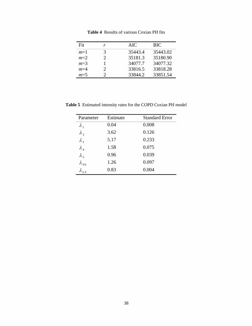
38

Table 4 Results of various Coxian PH fits

Fit r AIC BIC

m=1 3 35443.4 35443.02

m=2 2 35181.3 35180.90

m=3 1 34077.7 34077.32

m=4 2 33816.5 33818.28

m=5 2 33844.2 33851.54

Table 5 Estimated intensity rates for the COPD Coxian PH model

Parameter Estimate Standard Error

1 0.04 0.008

2 3.62 0.126

3 5.17 0.233

4 1.58 0.075

5 0.96 0.039

SS 1.26 0.097

LS 0.83 0.004

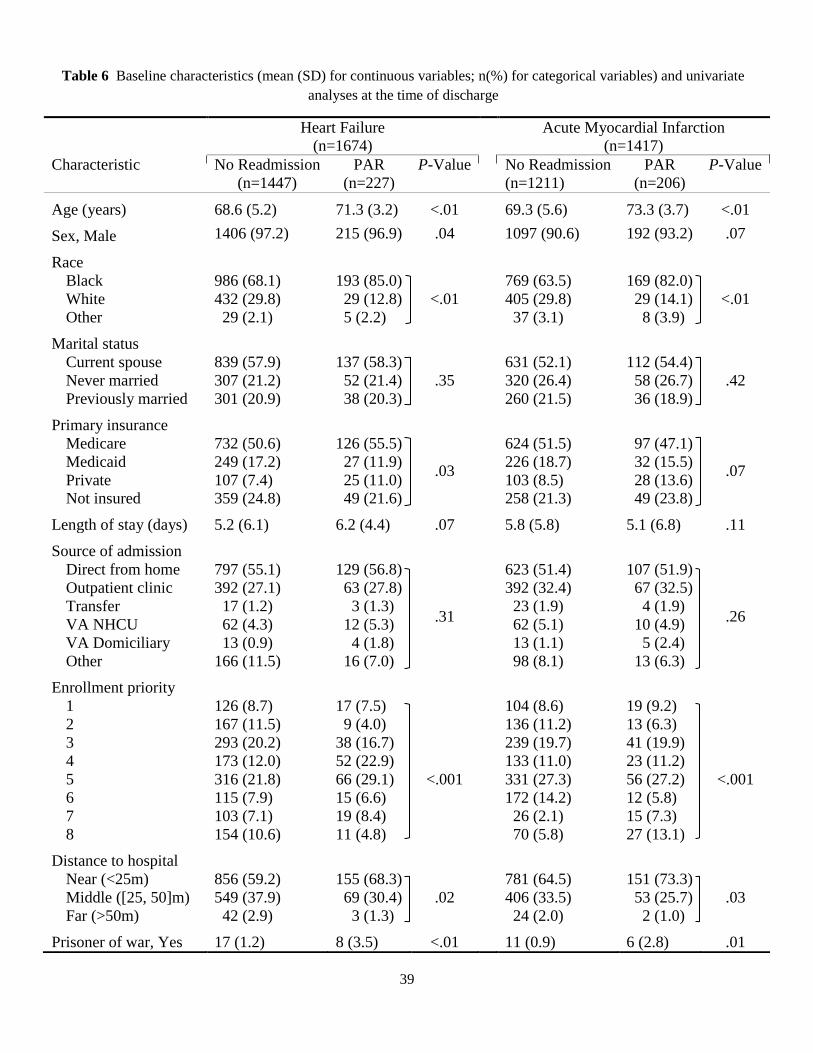
39

Heart Failure

(n=1674)

Acute Myocardial Infarction

(n=1417)

Characteristic No Readmission

(n=1447)

PAR

(n=227)

P-Value

No Readmission

(n=1211)

PAR

(n=206)

P-Value

Age (years) 68.6 (5.2) 71.3 (3.2) <.01 69.3 (5.6) 73.3 (3.7) <.01

Sex, Male 1406 (97.2) 215 (96.9) .04 1097 (90.6) 192 (93.2) .07

Race

Black

White

Other

986 (68.1)

432 (29.8)

29 (2.1)

193 (85.0)

29 (12.8)

5 (2.2)

<.01

769 (63.5)

405 (29.8)

37 (3.1)

169 (82.0)

29 (14.1)

8 (3.9)

<.01

Marital status

Current spouse

Never married

Previously married

839 (57.9)

307 (21.2)

301 (20.9)

137 (58.3)

52 (21.4)

38 (20.3)

.35

631 (52.1)

320 (26.4)

260 (21.5)

112 (54.4)

58 (26.7)

36 (18.9)

.42

Primary insurance

Medicare

Medicaid

Private

Not insured

732 (50.6)

249 (17.2)

107 (7.4)

359 (24.8)

126 (55.5)

27 (11.9)

25 (11.0)

49 (21.6)

.03

624 (51.5)

226 (18.7)

103 (8.5)

258 (21.3)

97 (47.1)

32 (15.5)

28 (13.6)

49 (23.8)

.07

Length of stay (days) 5.2 (6.1) 6.2 (4.4) .07 5.8 (5.8) 5.1 (6.8) .11

Source of admission

Direct from home

Outpatient clinic

Transfer

VA NHCU

VA Domiciliary

Other

797 (55.1)

392 (27.1)

17 (1.2)

62 (4.3)

13 (0.9)

166 (11.5)

129 (56.8)

63 (27.8)

3 (1.3)

12 (5.3)

4 (1.8)

16 (7.0)

.31

623 (51.4)

392 (32.4)

23 (1.9)

62 (5.1)

13 (1.1)

98 (8.1)

107 (51.9)

67 (32.5)

4 (1.9)

10 (4.9)

5 (2.4)

13 (6.3)

.26

Enrollment priority

1

2

3

4

5

6

7

8

126 (8.7)

167 (11.5)

293 (20.2)

173 (12.0)

316 (21.8)

115 (7.9)

103 (7.1)

154 (10.6)

17 (7.5)

9 (4.0)

38 (16.7)

52 (22.9)

66 (29.1)

15 (6.6)

19 (8.4)

11 (4.8)

<.001

104 (8.6)

136 (11.2)

239 (19.7)

133 (11.0)

331 (27.3)

172 (14.2)

26 (2.1)

70 (5.8)

19 (9.2)

13 (6.3)

41 (19.9)

23 (11.2)

56 (27.2)

12 (5.8)

15 (7.3)

27 (13.1)

<.001

Distance to hospital

Near (<25m)

Middle ([25, 50]m)

Far (>50m)

856 (59.2)

549 (37.9)

42 (2.9)

155 (68.3)

69 (30.4)

3 (1.3)

.02

781 (64.5)

406 (33.5)

24 (2.0)

151 (73.3)

53 (25.7)

2 (1.0)

.03

Prisoner of war, Yes 17 (1.2) 8 (3.5) <.01 11 (0.9) 6 (2.8) .01

Table 6 Baseline characteristics (mean (SD) for continuous variables; n(%) for categorical variables) and univariate

analyses at the time of discharge

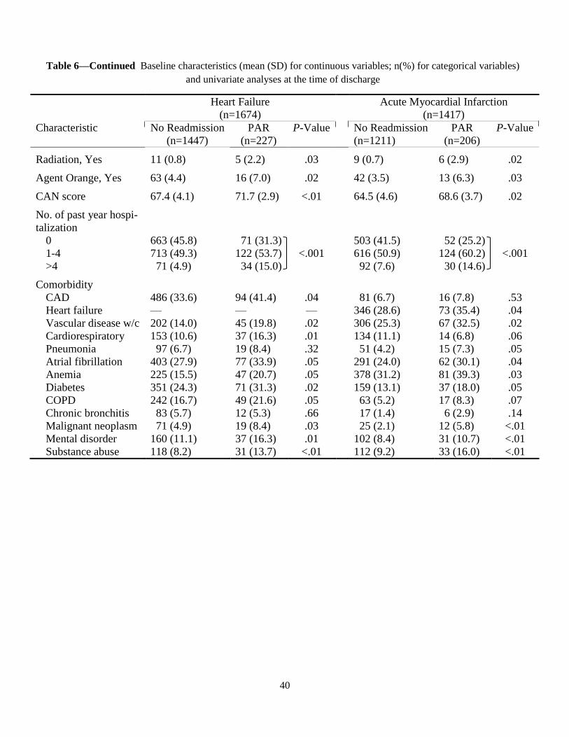
40

Heart Failure

(n=1674)

Acute Myocardial Infarction

(n=1417)

Characteristic No Readmission

(n=1447)

PAR

(n=227)

P-Value

No Readmission

(n=1211)

PAR

(n=206)

P-Value

Radiation, Yes 11 (0.8) 5 (2.2) .03 9 (0.7) 6 (2.9) .02

Agent Orange, Yes 63 (4.4) 16 (7.0) .02 42 (3.5) 13 (6.3) .03

CAN score 67.4 (4.1) 71.7 (2.9) <.01 64.5 (4.6) 68.6 (3.7) .02

No. of past year hospi-

talization

0

1-4

>4

663 (45.8)

713 (49.3)

71 (4.9)

71 (31.3)

122 (53.7)

34 (15.0)

<.001

503 (41.5)

616 (50.9)

92 (7.6)

52 (25.2)

124 (60.2)

30 (14.6)

<.001

Comorbidity

CAD

Heart failure

Vascular disease w/c

Cardiorespiratory

Pneumonia

Atrial fibrillation

Anemia

Diabetes

COPD

Chronic bronchitis

Malignant neoplasm

Mental disorder

Substance abuse

486 (33.6)

—

202 (14.0)

153 (10.6)

97 (6.7)

403 (27.9)

225 (15.5)

351 (24.3)

242 (16.7)

83 (5.7)

71 (4.9)

160 (11.1)

118 (8.2)

94 (41.4)

—

45 (19.8)

37 (16.3)

19 (8.4)

77 (33.9)

47 (20.7)

71 (31.3)

49 (21.6)

12 (5.3)

19 (8.4)

37 (16.3)

31 (13.7)

.04

—

.02

.01

.32

.05

.05

.02

.05

.66

.03

.01

<.01

81 (6.7)

346 (28.6)

306 (25.3)

134 (11.1)

51 (4.2)

291 (24.0)

378 (31.2)

159 (13.1)

63 (5.2)

17 (1.4)

25 (2.1)

102 (8.4)

112 (9.2)

16 (7.8)

73 (35.4)

67 (32.5)

14 (6.8)

15 (7.3)

62 (30.1)

81 (39.3)

37 (18.0)

17 (8.3)

6 (2.9)

12 (5.8)

31 (10.7)

33 (16.0)

.53

.04

.02

.06

.05

.04

.03

.05

.07

.14

<.01

<.01

<.01

Table 6—Continued Baseline characteristics (mean (SD) for continuous variables; n(%) for categorical variables)

and univariate analyses at the time of discharge

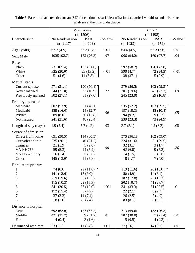
41

Pneumonia

(n=1306)

COPD

(n=1198)

Characteristic No Readmission

(n=1117)

PAR

(n=189)

P-Value

No Readmission

(n=1025)

PAR

(n=173)

P-Value

Age (years) 67.7 (4.9) 68.3 (2.8) <.01 63.6 (4.5) 65.3 (2.6) <.01

Sex, Male 1035 (92.7) 182 (96.3) .07 966 (94.2) 169 (97.7) .04

Race

Black

White

Other

731 (65.4)

335 (30.0)

51 (4.6)

153 (81.0)

25 (13.2)

11 (5.8)

<.01

597 (58.2)

390 (4.7)

38 (37.1)

126 (72.8)

42 (24.3)

5 (2.9)

<.01

Marital status

Current spouse

Never married

Previously married

571 (51.1)

244 (21.8)

302 (27.1)

106 (56.1)

32 (16.9)

51 (27.0)

.27

579 (56.5)

201 (19.6)

245 (23.9)

103 (59.5)

41 (23.7)

29 (16.8)

.09

Primary insurance

Medicare

Medicaid

Private

Not insured

602 (53.9)

185 (16.6)

89 (8.0)

241 (21.6)

91 (48.1)

24 (12.7)

26 (13.8)

48 (25.4)

.06

535 (52.2)

157 (15.3)

94 (9.2)

239 (23.3)

103 (59.5)

18 (10.4)

9 (5.2)

43 (24.9)

.05

Length of stay (days) 4.9 (5.4) 5.7 (4.2) .03 3.7 (5.1) 4.3 (3.2) .08

Source of admission

Direct from home

Outpatient clinic

Transfer

VA NHCU

VA Domiciliary

Other

651 (58.3)

225 (20.1)

21 (1.9)

59 (5.3)

16 (1.4)

145 (13.0)

114 (60.3)

40 (21.2)

5 (2.6)

14 (7.4)

5 (2.6)

11 (5.8)

.09

575 (56.1)

324 (31.6)

32 (3.1)

62 (6.0)

14 (1.5)

18 (1.7)

102 (59.0)

51 (29.5)

3 (1.7)

9 (5.2)

1 (0.6)

7 (4.0)

.36

Enrollment priority

1

2

3

4

5

6

7

8

74 (6.6)

141 (12.6)

219 (19.6)

115 (10.3)

341 (30.5)

172 (15.4)

37 (3.3)

18 (1.6)

22 (11.6)

17 (9.0)

35 (18.5)

29 (15.3)

36 (19.0)

8 (4.2)

14 (7.4)

28 (7.4)

<.001

119 (11.6)

50 (4.9)

182 (17.8)

202 (19.7)

341 (33.3)

22 (2.1)

26 (2.5)

83 (8.1)

26 (15.0)

14 (8.1)

23 (13.3)

41 (23.7)

51 (29.5)

5 (2.9)

7 (4.0)

6 (3.5)

.01

Distance to hospital

Near

Middle

Far

692 (62.0)

421 (37.7)

4 (0.4)

127 (67.2)

59 (31.2)

3 (1.6)

.01

713 (69.6)

307 (30.0)

5 (0.5)

132 (76.3)

37 (21.4)

4 (2.3)

<.01

Prisoner of war, Yes 23 (2.1) 11 (5.8) <.01 27 (2.6) 14 (8.1) <.01

Table 7 Baseline characteristics (mean (SD) for continuous variables; n(%) for categorical variables) and univariate

analyses at the time of discharge

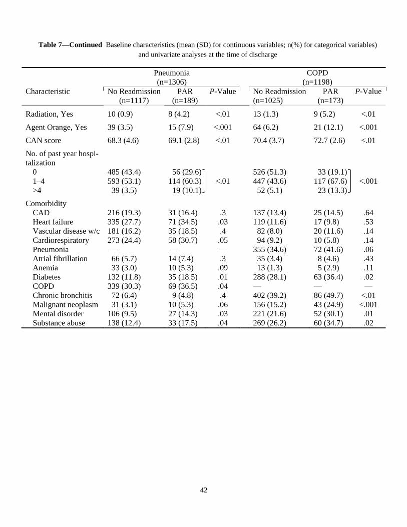
42

Pneumonia

(n=1306)

COPD

(n=1198)

Characteristic No Readmission

(n=1117)

PAR

(n=189)

P-Value

No Readmission

(n=1025)

PAR

(n=173)

P-Value

Radiation, Yes 10 (0.9) 8 (4.2) <.01 13 (1.3) 9 (5.2) <.01

Agent Orange, Yes 39 (3.5) 15 (7.9) <.001 64 (6.2) 21 (12.1) <.001

CAN score 68.3 (4.6) 69.1 (2.8) <.01 70.4 (3.7) 72.7 (2.6) <.01

No. of past year hospi-

talization

0

1–4

>4

485 (43.4)

593 (53.1)

39 (3.5)

56 (29.6)

114 (60.3)

19 (10.1)

<.01

526 (51.3)

447 (43.6)

52 (5.1)

33 (19.1)

117 (67.6)

23 (13.3)

<.001

Comorbidity

CAD

Heart failure

Vascular disease w/c

Cardiorespiratory

Pneumonia

Atrial fibrillation

Anemia

Diabetes

COPD

Chronic bronchitis

Malignant neoplasm

Mental disorder

Substance abuse

216 (19.3)

335 (27.7)

181 (16.2)

273 (24.4)

—

66 (5.7)

33 (3.0)

132 (11.8)

339 (30.3)

72 (6.4)

31 (3.1)

106 (9.5)

138 (12.4)

31 (16.4)

71 (34.5)

35 (18.5)

58 (30.7)

—

14 (7.4)

10 (5.3)

35 (18.5)

69 (36.5)

9 (4.8)

10 (5.3)

27 (14.3)

33 (17.5)

.3

.03

.4

.05

—

.3

.09

.01

.04

.4

.06

.03

.04

137 (13.4)

119 (11.6)

82 (8.0)

94 (9.2)

355 (34.6)

35 (3.4)

13 (1.3)

288 (28.1)

—

402 (39.2)

156 (15.2)

221 (21.6)

269 (26.2)

25 (14.5)

17 (9.8)

20 (11.6)

10 (5.8)

72 (41.6)

8 (4.6)

5 (2.9)

63 (36.4)

—

86 (49.7)

43 (24.9)

52 (30.1)

60 (34.7)

.64

.53

.14

.14

.06

.43

.11

.02

—

<.01

<.001

.01

.02

Table 7—Continued Baseline characteristics (mean (SD) for continuous variables; n(%) for categorical variables)

and univariate analyses at the time of discharge

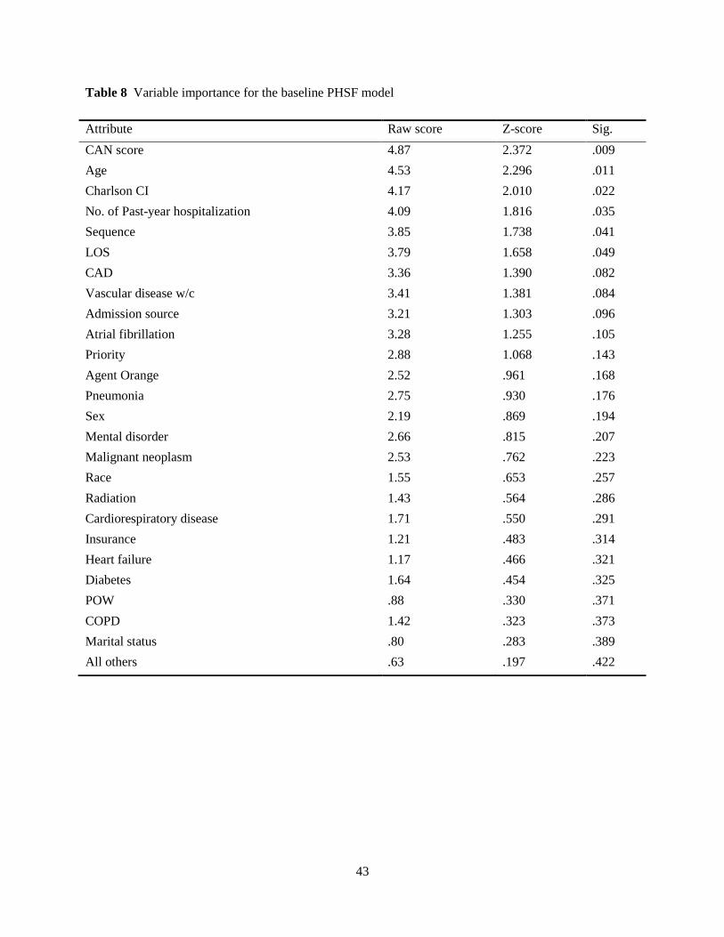
43

Table 8 Variable importance for the baseline PHSF model

Attribute Raw score Z-score Sig.

CAN score 4.87 2.372 .009

Age 4.53 2.296 .011

Charlson CI 4.17 2.010 .022

No. of Past-year hospitalization 4.09 1.816 .035

Sequence 3.85 1.738 .041

LOS 3.79 1.658 .049

CAD 3.36 1.390 .082

Vascular disease w/c 3.41 1.381 .084

Admission source 3.21 1.303 .096

Atrial fibrillation 3.28 1.255 .105

Priority 2.88 1.068 .143

Agent Orange 2.52 .961 .168

Pneumonia 2.75 .930 .176

Sex 2.19 .869 .194

Mental disorder 2.66 .815 .207

Malignant neoplasm 2.53 .762 .223

Race 1.55 .653 .257

Radiation 1.43 .564 .286

Cardiorespiratory disease 1.71 .550 .291

Insurance 1.21 .483 .314

Heart failure 1.17 .466 .321

Diabetes 1.64 .454 .325

POW .88 .330 .371

COPD 1.42 .323 .373

Marital status .80 .283 .389

All others .63 .197 .422

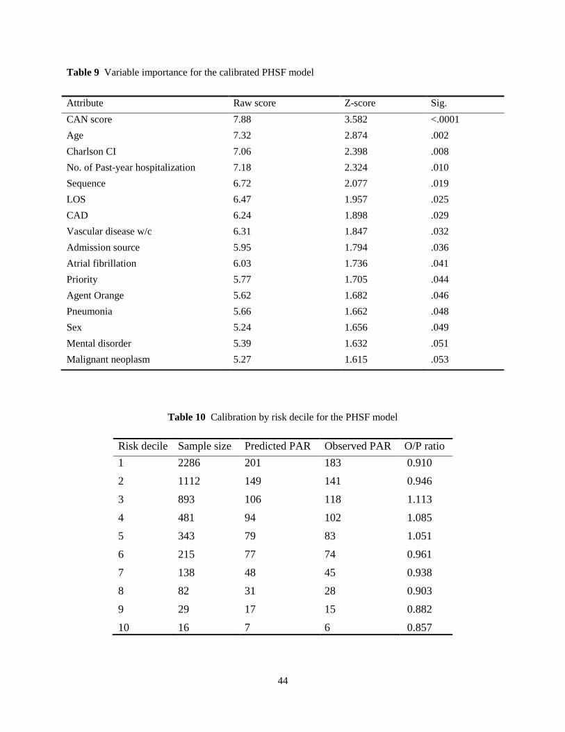
44

Table 9 Variable importance for the calibrated PHSF model

Table 10 Calibration by risk decile for the PHSF model

Risk decile Sample size Predicted PAR Observed PAR O/P ratio

1 2286 201 183 0.910

2 1112 149 141 0.946

3 893 106 118 1.113

4 481 94 102 1.085

5 343 79 83 1.051

6 215 77 74 0.961

7 138 48 45 0.938

8 82 31 28 0.903

9 29 17 15 0.882

10 16 7 6 0.857

Attribute Raw score Z-score Sig.

CAN score 7.88 3.582 <.0001

Age 7.32 2.874 .002

Charlson CI 7.06 2.398 .008

No. of Past-year hospitalization 7.18 2.324 .010

Sequence 6.72 2.077 .019

LOS 6.47 1.957 .025

CAD 6.24 1.898 .029

Vascular disease w/c 6.31 1.847 .032

Admission source 5.95 1.794 .036

Atrial fibrillation 6.03 1.736 .041

Priority 5.77 1.705 .044

Agent Orange 5.62 1.682 .046

Pneumonia 5.66 1.662 .048

Sex 5.24 1.656 .049

Mental disorder 5.39 1.632 .051

Malignant neoplasm 5.27 1.615 .053

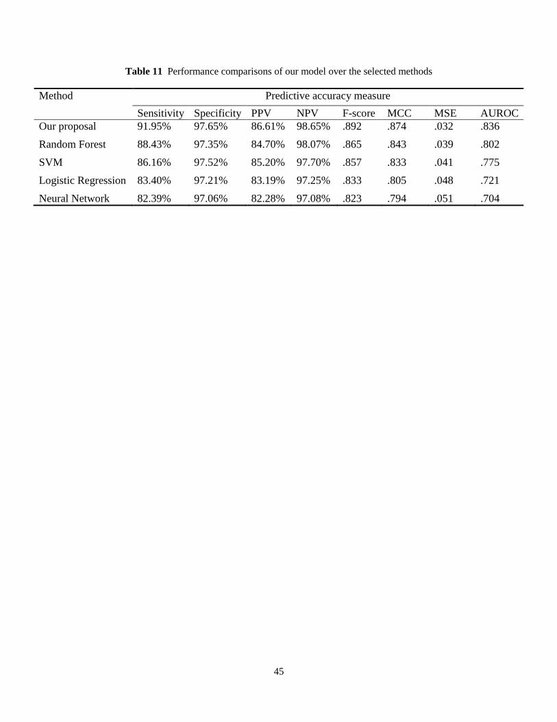
45

Table 11 Performance comparisons of our model over the selected methods

Method Predictive accuracy measure

Sensitivity Specificity PPV NPV F-score MCC MSE AUROC

Our proposal 91.95% 97.65% 86.61% 98.65% .892 .874 .032 .836

Random Forest 88.43% 97.35% 84.70% 98.07% .865 .843 .039 .802

SVM 86.16% 97.52% 85.20% 97.70% .857 .833 .041 .775

Logistic Regression 83.40% 97.21% 83.19% 97.25% .833 .805 .048 .721

Neural Network 82.39% 97.06% 82.28% 97.08% .823 .794 .051 .704