A Population Gain Control Model of Spatiotemporal Responses inthe Visual Cortex

Yiu Fai Sit

Report AI09-06 August 2009

yfsit@cs.utexas.eduhttp://www.cs.utexas.edu/users/nn/

Artificial Intelligence LaboratoryThe University of Texas at Austin

Austin, TX 78712

Copyright

by

Yiu Fai Sit

2009

The Dissertation Committee for Yiu Fai Sitcertifies that this is the approved version of the following dissertation:

A Population Gain Control Model of Spatiotemporal Responses inthe Visual Cortex

Committee:

Risto Miikkulainen, Supervisor

Eyal Seidemann, Supervisor

James Bednar

Benjamin Kuipers

Raymond Mooney

Peter Stone

A Population Gain Control Model of Spatiotemporal Responses in

the Visual Cortex

by

Yiu Fai Sit, B.Eng.; M.Phil.

Dissertation

Presented to the Faculty of the Graduate School of

The University of Texas at Austin

in Partial Fulfillment

of the Requirements

for the Degree of

Doctor of Philosophy

The University of Texas at Austin

August 2009

AcknowledgmentsThis dissertation would not have been possible without the guidance and support of my advisers, Eyal Seide-mann and Risto Miikkulainen. Eyal is an outstanding mentor and scientist. I could not have accomplishedwhat I did without his insightful suggestions, critical comments, and excellent advice throughout this re-search. Risto has been a constant source of encouragement, inspiration, and motivation during my wholegraduate career. My interest in computational neuroscience finds deep roots in his work and this dissertationwould not even have started without his introduction to this field.

A special thank you must go to Bill Geisler. Bill is one of the pioneers who laid the foundation ofthis work. I am grateful for his invaluable ideas and feedback throughout this research, not to mention allthe improvements that he made in the revisions of our paper.

I would also like to thank all the friends and colleagues in Eyal’s and Risto’s labs for their discus-sions, comments, and questions, especially Yuzhi Chen and Bill Bosking. Yuzhi did all the experiments withthe monkeys described in the first half of this dissertation and has contributed many ideas to my work. Thelateral interactions experiments were done by Bill, who had provided many helpful comments and adviceon various projects. I also thank Zhiyong Yang for collecting the data for the moving stimuli.

I thank my wonderful family for their support throughout my study. I am very fortunate to have aloving family and I am grateful for all their faith and trust in me. Finally, I thank my wife, Yoee, for her loveand patience that keep this long-distance relationship lively and fresh.

YIU FAI SIT

The University of Texas at AustinAugust 2009

v

A Population Gain Control Model of Spatiotemporal Responses in

the Visual Cortex

Publication No.

Yiu Fai Sit, Ph.D.The University of Texas at Austin, 2009

Supervisors: Risto Miikkulainen, Eyal Seidemann

The mammalian brain is a complex computing system that contains billions of neurons and trillions ofconnections. Is there a general principle that governs the processing in such large neural populations? Thisdissertation attempts to address this question using computational modeling and quantitative analysis ofdirect physiological measurements of large neural populations in the monkey primary visual cortex (V1).First, the complete spatiotemporal dynamics of V1 responses over the entire region that is activated bysmall stationary stimuli are characterized quantitatively. The dynamics of the responses are found to besystematic but complex. Importantly, they are inconsistent with many popular computational models ofneural processing. Second, a simple population gain control (PGC) model that can account for these complexresponse properties is proposed for the small stationary stimuli. The PGC model is then used to predict theresponses to stimuli composed of two elements and stimuli that move at a constant speed. The predictions ofthe model are consistent with the measured responses in V1 for both stimuli. PGC is the first model that canaccount for the complete spatiotemporal dynamics of V1 population responses for different types of stimuli,suggesting that gain control is a general mechanism of neural processing.

vi

Contents

Acknowledgments v

Abstract vi

Contents vii

List of Figures x

Chapter 1 Introduction 11.1 Motivation . . . . . . . . . . . . . . . . . . . . . . . . . . . . . . . . . . . . . . . . . . . . 11.2 Approach . . . . . . . . . . . . . . . . . . . . . . . . . . . . . . . . . . . . . . . . . . . . 21.3 Outline of the dissertation . . . . . . . . . . . . . . . . . . . . . . . . . . . . . . . . . . . . 3

Chapter 2 Background 42.1 The early visual pathway . . . . . . . . . . . . . . . . . . . . . . . . . . . . . . . . . . . . 4

2.1.1 Retina . . . . . . . . . . . . . . . . . . . . . . . . . . . . . . . . . . . . . . . . . . 42.1.2 Lateral geniculate nucleus (LGN) . . . . . . . . . . . . . . . . . . . . . . . . . . . 42.1.3 Primary visual cortex (V1) . . . . . . . . . . . . . . . . . . . . . . . . . . . . . . . 5

2.2 Population responses in V1 . . . . . . . . . . . . . . . . . . . . . . . . . . . . . . . . . . . 72.3 Voltage-sensitive dye imaging (VSDI) . . . . . . . . . . . . . . . . . . . . . . . . . . . . . 72.4 Hodgkin-Huxley model . . . . . . . . . . . . . . . . . . . . . . . . . . . . . . . . . . . . . 92.5 Conclusion . . . . . . . . . . . . . . . . . . . . . . . . . . . . . . . . . . . . . . . . . . . 10

Chapter 3 Related Work 113.1 Motivation . . . . . . . . . . . . . . . . . . . . . . . . . . . . . . . . . . . . . . . . . . . . 113.2 Models with linear instantaneous input summation . . . . . . . . . . . . . . . . . . . . . . 11

3.2.1 Linear-nonlinear (LN) models . . . . . . . . . . . . . . . . . . . . . . . . . . . . . 113.2.2 Push-pull effect of excitation and inhibition . . . . . . . . . . . . . . . . . . . . . . 123.2.3 Spatially organized LN units . . . . . . . . . . . . . . . . . . . . . . . . . . . . . . 133.2.4 Modeling lateral propagation with the LN model . . . . . . . . . . . . . . . . . . . 13

3.3 Models with temporal integration of inputs . . . . . . . . . . . . . . . . . . . . . . . . . . . 133.3.1 Leaky integrate-and-fire (LIF) model . . . . . . . . . . . . . . . . . . . . . . . . . 133.3.2 Spatially organized leaky integrators . . . . . . . . . . . . . . . . . . . . . . . . . . 15

3.4 Normalization gain control models . . . . . . . . . . . . . . . . . . . . . . . . . . . . . . . 163.5 Conclusion . . . . . . . . . . . . . . . . . . . . . . . . . . . . . . . . . . . . . . . . . . . 17

vii

Chapter 4 Population Responses in the Monkey Primary Visual Cortex 184.1 Motivation . . . . . . . . . . . . . . . . . . . . . . . . . . . . . . . . . . . . . . . . . . . . 184.2 Measuring population responses with voltage-sensitive dye imaging (VSDI) . . . . . . . . . 18

4.2.1 Behavioral task and visual stimuli . . . . . . . . . . . . . . . . . . . . . . . . . . . 194.2.2 Analysis of imaging data . . . . . . . . . . . . . . . . . . . . . . . . . . . . . . . . 19

4.3 Population responses to a Gabor stimulus in V1 . . . . . . . . . . . . . . . . . . . . . . . . 204.3.1 Peak responses . . . . . . . . . . . . . . . . . . . . . . . . . . . . . . . . . . . . . 204.3.2 Overview of the temporal response properties at different locations . . . . . . . . . 224.3.3 Properties of the rising edge . . . . . . . . . . . . . . . . . . . . . . . . . . . . . . 244.3.4 Properties of the falling edge . . . . . . . . . . . . . . . . . . . . . . . . . . . . . . 28

4.4 Discussion . . . . . . . . . . . . . . . . . . . . . . . . . . . . . . . . . . . . . . . . . . . . 284.5 Conclusion . . . . . . . . . . . . . . . . . . . . . . . . . . . . . . . . . . . . . . . . . . . 28

Chapter 5 Population Gain Control Model 315.1 Population gain control (PGC) model . . . . . . . . . . . . . . . . . . . . . . . . . . . . . 31

5.1.1 Transforming visual stimuli to model input . . . . . . . . . . . . . . . . . . . . . . 335.1.2 Processing in the model units . . . . . . . . . . . . . . . . . . . . . . . . . . . . . 335.1.3 General behavior of a model stage . . . . . . . . . . . . . . . . . . . . . . . . . . . 345.1.4 Response transformation between stages . . . . . . . . . . . . . . . . . . . . . . . . 36

5.2 Effects of normalization pool size . . . . . . . . . . . . . . . . . . . . . . . . . . . . . . . 365.3 Parameter estimation . . . . . . . . . . . . . . . . . . . . . . . . . . . . . . . . . . . . . . 375.4 Simulation of VSDI responses . . . . . . . . . . . . . . . . . . . . . . . . . . . . . . . . . 38

5.4.1 Results of the simulation . . . . . . . . . . . . . . . . . . . . . . . . . . . . . . . . 385.5 Relative normalization strengths in the different stages . . . . . . . . . . . . . . . . . . . . 395.6 Discussion . . . . . . . . . . . . . . . . . . . . . . . . . . . . . . . . . . . . . . . . . . . . 41

5.6.1 Modeling population responses . . . . . . . . . . . . . . . . . . . . . . . . . . . . 415.6.2 Possible implementation of divisive population gain control . . . . . . . . . . . . . 425.6.3 Relationship between the responses of a single neuron and a neural population . . . 425.6.4 Importance of combined quantitative analysis and modeling . . . . . . . . . . . . . 43

5.7 Conclusion . . . . . . . . . . . . . . . . . . . . . . . . . . . . . . . . . . . . . . . . . . . 43

Chapter 6 Spatial Interactions Between Visual Stimuli 456.1 Motivation . . . . . . . . . . . . . . . . . . . . . . . . . . . . . . . . . . . . . . . . . . . . 456.2 Interaction of two elements . . . . . . . . . . . . . . . . . . . . . . . . . . . . . . . . . . . 46

6.2.1 Input to the model . . . . . . . . . . . . . . . . . . . . . . . . . . . . . . . . . . . 466.2.2 Qualitative analysis of the model . . . . . . . . . . . . . . . . . . . . . . . . . . . . 476.2.3 Results of simulation . . . . . . . . . . . . . . . . . . . . . . . . . . . . . . . . . . 486.2.4 Results of VSDI experiments . . . . . . . . . . . . . . . . . . . . . . . . . . . . . . 55

6.3 Center-surround interactions . . . . . . . . . . . . . . . . . . . . . . . . . . . . . . . . . . 596.3.1 Predictions of the model on the responses at stimulus center . . . . . . . . . . . . . 60

6.4 Behavioral predictions . . . . . . . . . . . . . . . . . . . . . . . . . . . . . . . . . . . . . 616.4.1 A simple decoder . . . . . . . . . . . . . . . . . . . . . . . . . . . . . . . . . . . . 626.4.2 Two-element stimuli . . . . . . . . . . . . . . . . . . . . . . . . . . . . . . . . . . 626.4.3 Center-surround stimuli . . . . . . . . . . . . . . . . . . . . . . . . . . . . . . . . 63

viii

6.4.4 Proposed psychophysical experiments with VSDI . . . . . . . . . . . . . . . . . . . 666.4.5 Summary . . . . . . . . . . . . . . . . . . . . . . . . . . . . . . . . . . . . . . . . 68

6.5 Conclusion . . . . . . . . . . . . . . . . . . . . . . . . . . . . . . . . . . . . . . . . . . . 68

Chapter 7 Spatiotemporal Interactions Between Visual Stimuli 707.1 Motivation . . . . . . . . . . . . . . . . . . . . . . . . . . . . . . . . . . . . . . . . . . . . 707.2 Spatiotemporal stimuli . . . . . . . . . . . . . . . . . . . . . . . . . . . . . . . . . . . . . 707.3 Results of the model . . . . . . . . . . . . . . . . . . . . . . . . . . . . . . . . . . . . . . 71

7.3.1 Input to the model . . . . . . . . . . . . . . . . . . . . . . . . . . . . . . . . . . . 717.3.2 Qualitative analysis . . . . . . . . . . . . . . . . . . . . . . . . . . . . . . . . . . . 747.3.3 Simulation results . . . . . . . . . . . . . . . . . . . . . . . . . . . . . . . . . . . 74

7.4 VSDI experiment . . . . . . . . . . . . . . . . . . . . . . . . . . . . . . . . . . . . . . . . 787.4.1 Experimental procedures and data analysis . . . . . . . . . . . . . . . . . . . . . . 787.4.2 Results . . . . . . . . . . . . . . . . . . . . . . . . . . . . . . . . . . . . . . . . . 79

7.5 Discussion . . . . . . . . . . . . . . . . . . . . . . . . . . . . . . . . . . . . . . . . . . . . 837.5.1 Model parameters . . . . . . . . . . . . . . . . . . . . . . . . . . . . . . . . . . . . 83

7.6 Conclusion . . . . . . . . . . . . . . . . . . . . . . . . . . . . . . . . . . . . . . . . . . . 84

Chapter 8 Discussion and Future Research 858.1 Model parameters . . . . . . . . . . . . . . . . . . . . . . . . . . . . . . . . . . . . . . . . 858.2 Extension to fine spatial scales . . . . . . . . . . . . . . . . . . . . . . . . . . . . . . . . . 86

8.2.1 Modeling orientation-specific signals in lateral and feedback connections . . . . . . 868.2.2 Possible extensions of the PGC model for orientation-specific signals . . . . . . . . 87

8.3 Analysis of the extended model . . . . . . . . . . . . . . . . . . . . . . . . . . . . . . . . . 888.4 Decoding orientation-specific neural response . . . . . . . . . . . . . . . . . . . . . . . . . 888.5 Network implementation of the model . . . . . . . . . . . . . . . . . . . . . . . . . . . . . 898.6 Modeling higher level areas . . . . . . . . . . . . . . . . . . . . . . . . . . . . . . . . . . . 898.7 Conclusion . . . . . . . . . . . . . . . . . . . . . . . . . . . . . . . . . . . . . . . . . . . 89

Chapter 9 Conclusion 919.1 Contributions . . . . . . . . . . . . . . . . . . . . . . . . . . . . . . . . . . . . . . . . . . 919.2 Conclusion . . . . . . . . . . . . . . . . . . . . . . . . . . . . . . . . . . . . . . . . . . . 92

Bibliography 93

Vita 102

ix

List of Figures

2.1 The early visual pathway. . . . . . . . . . . . . . . . . . . . . . . . . . . . . . . . . . . . . 52.2 Receptive fields of the retinal ganglion cells and LGN cells. . . . . . . . . . . . . . . . . . . 52.3 Spatial receptive fields of V1 neurons. . . . . . . . . . . . . . . . . . . . . . . . . . . . . . 62.4 Voltage-sensitive dye imaging with an awake and behaving monkey. . . . . . . . . . . . . . 82.5 The Hodgkin-Huxley model. . . . . . . . . . . . . . . . . . . . . . . . . . . . . . . . . . . 9

3.1 Models with instantaneous linear summation of input. . . . . . . . . . . . . . . . . . . . . . 123.2 Temporal integration of inputs and spike generation. . . . . . . . . . . . . . . . . . . . . . . 143.3 A normalization gain control model. . . . . . . . . . . . . . . . . . . . . . . . . . . . . . . 16

4.1 The task performed by the monkey. . . . . . . . . . . . . . . . . . . . . . . . . . . . . . . . 194.2 Peak responses to a Gabor stimulus. . . . . . . . . . . . . . . . . . . . . . . . . . . . . . . 214.3 Temporal responses to different stimulus contrasts at the center. . . . . . . . . . . . . . . . . 234.4 Spatiotemporal responses to different stimulus contrasts. . . . . . . . . . . . . . . . . . . . 244.5 Temporal properties of the rising edge. . . . . . . . . . . . . . . . . . . . . . . . . . . . . . 254.6 Effects of lateral propagation on the latency of the rising edge. . . . . . . . . . . . . . . . . 274.7 Temporal properties of the falling edge. . . . . . . . . . . . . . . . . . . . . . . . . . . . . 29

5.1 A canonical model of visual processing. . . . . . . . . . . . . . . . . . . . . . . . . . . . . 325.2 Peak responses of the second stage in the model. . . . . . . . . . . . . . . . . . . . . . . . 395.3 Spatiotemporal responses of second stage in the model. . . . . . . . . . . . . . . . . . . . . 405.4 Predictions of the size tuning curves of five combinations of normalization strengths. . . . . 41

6.1 Stimuli for studying interactions between elements. . . . . . . . . . . . . . . . . . . . . . . 466.2 Spatial profiles for stimuli consisting of a 10% and a 100% contrast element. . . . . . . . . . 496.3 Spatial profiles for stimuli containing 25% contrast elements. . . . . . . . . . . . . . . . . . 516.4 Spatial profiles for stimuli containing 5% contrast elements. . . . . . . . . . . . . . . . . . 526.5 Different regimes of the interactions at the center of G0. . . . . . . . . . . . . . . . . . . . 546.6 Spatial VSDI responses for stimuli containing a 10% and a 100% contrast element. . . . . . 566.7 Spatial VSDI responses for stimuli consisting of elements at 25% contrast. . . . . . . . . . . 586.8 Spatial VSDI responses for stimuli consisting of elements with 0.75◦ separation. . . . . . . 596.9 Example center-surround stimuli. . . . . . . . . . . . . . . . . . . . . . . . . . . . . . . . . 606.10 Different regimes of interactions when the contrasts of the elements are varied. . . . . . . . 616.11 Detection threshold for two-element stimuli (50-150 ms window). . . . . . . . . . . . . . . 646.12 Detection threshold for two-element stimuli (150-250 ms window). . . . . . . . . . . . . . . 65

x

6.13 Time course and spatial profiles at different time points. . . . . . . . . . . . . . . . . . . . . 666.14 Detection threshold for center-surround stimuli (50-150 ms window). . . . . . . . . . . . . 676.15 Detection threshold for center-surround stimuli (150-250 ms window). . . . . . . . . . . . . 67

7.1 Counterclockwise spatiotemporal stimuli in the VSDI experiment. . . . . . . . . . . . . . . 727.2 Clockwise spatiotemporal stimuli in the VSDI experiment. . . . . . . . . . . . . . . . . . . 737.3 Retinotopic mapping of the stimulus. . . . . . . . . . . . . . . . . . . . . . . . . . . . . . . 737.4 Spatiotemporal responses of the model for the counterclockwise stimuli. . . . . . . . . . . . 767.5 Spatiotemporal responses of the model for the clockwise stimuli. . . . . . . . . . . . . . . . 777.6 Relative latencies of the responses. . . . . . . . . . . . . . . . . . . . . . . . . . . . . . . . 787.7 Normalized peak spatial responses for the three single-wedge stimuli. . . . . . . . . . . . . 807.8 Spatiotemporal VSDI responses for the counterclockwise stimuli. . . . . . . . . . . . . . . 817.9 Spatiotemporal VSDI responses for the clockwise stimuli. . . . . . . . . . . . . . . . . . . 827.10 Relative latencies of the VSDI responses and the model’s predictions. . . . . . . . . . . . . 83

xi

Chapter 1

Introduction

The mammalian brain is a complex computing system. It contains billions of neurons, each of which is anonlinear computing unit that connects with thousands of neurons. Such complexity is fascinating, but atthe same time it makes understanding the brain one of the hardest problems in science. Are there generalprinciples for the computation in the brain? Is it even possible to find one?

The goal of this dissertation is to uncover such a principle for how large neural populations, such asthe primary visual cortex (V1), respond to canonical stimuli. In order to do that, empirical measurementsof responses in V1 will be combined with computational simulations. The result will be a computationaltheory that can be used to understand processing at the population level in many areas of the cortex.

1.1 Motivation

The traditional approach to understand neural processing is to study the individual components of the brain,i.e. single neurons. By observing the change in response as some feature in the stimulus varies, the compu-tation performed by the neuron can be characterized. However, given the interconnected nature of the brain,a neuron’s response is hardly due to the stimuli alone. Any neuron that connects to it, directly or indirectly,can affect its response. A neuron’s response is therefore only a part of the computation carried out by a largeneural population. Single-unit responses can therefore only provide a partial picture of the processing in thebrain.

A more appropriate approach to study neural computation is to measure the responses of a largepopulation of neurons simultaneously and directly. Although population responses can potentially be es-timated from the results of single-unit recordings, neurons are interconnected and vastly heterogeneous.It is thus unclear how these properties are combined and manifested at the population level. In addition,population responses need to be measured at high spatial and temporal resolution to capture their dynamicsaccurately. For instance, hemodynamic responses measured by fMRI and intrinsic optical imaging are tooslow for characterizing the dynamics. However, optical imaging can be combined with voltage-sensitivedyes, achieving temporal resolution at the millisecond range. The first main contribution of this disserta-tion is to use such voltage-sensitive dye imaging (VSDI; Grinvald & Hildesheim, 2004) to provide the firstcomplete quantitative description of the dynamics of population responses for simple stimuli.

Based on the population responses, it is then possible to search for the general principles of compu-tation in the brain. A computational model is a formal hypothesis of how the observed response dynamicsarise. If the hypothesis reflects a general mechanism, its predictions should be consistent with the neural

1

responses for a variety of stimuli. For instance, the Hodgkin-Huxley model (Hodgkin & Huxley, 1952) ishighly successful in this regard. It explains and predicts the dynamics of an individual neuron accurately(De Schutter & Bower, 1994a, 1994b; Mainen & Sejnowski, 1998), setting the standard for what a computa-tional model should accomplish. However, as in traditional studies of neural responses, the Hodgkin-Huxleymodel and its extensions apply only to a single neuron or a few neurons. They are not as effective for a largeneural population, because they require a large number of parameters.

To understand the processing of a neural population, models with a higher level of abstraction arerequired. However, in contrast to the Hodgkin-Huxley model, most large-scale models of neural popula-tions either do not take the response dynamics into account (Miikkulainen, Bednar, Choe, & Sirosh, 2005;Sit & Miikkulainen, 2009), or ignore some of the nonlinearities of the response (Ben-Yishai, Bar-Or, &Sompolinsky, 1995; Somers, Nelson, & Sur, 1995; Hansel & Sompolinsky, 1998). A new class of compu-tational models that operates at the population level and takes the response dynamics and nonlinearity intoaccount is therefore needed to understand processing at the population level in the brain. The second maincontribution of this dissertation is to provide such a model. The aim is to create a standard model for neuralpopulations, similar to what the Hodgkin-Huxley model is of single neurons.

1.2 Approach

To provide the foundation for the model, VSDI is used in this dissertation to measure population responsesin the macaque primary visual cortex (V1) from the entire spatial region of activity at high spatial andtemporal resolution for brief, localized stimuli. The spatiotemporal dynamics of these responses are thusquantitatively characterized for the first time.

Next, this dissertation considers whether there is a general mechanism that can account for thedynamics of V1 population responses over the entire active region. Different computational models thathave been proposed in the past are tested using the stimuli in the VSDI experiment as input. Most of themare found to be inconsistent with the observed response properties.

To account for the observed properties in both time and space, this dissertation then proposes apopulation gain control (PGC) model that generalizes earlier normalization models for single neurons inthe LGN (Shapley & Victor, 1978; Victor, 1987; Bonin, Mante, & Carandini, 2005) and V1 (Albrecht &Geisler, 1991; Heeger, 1992; Carandini, Heeger, & Movshon, 1997; Mante, Bonin, & Carandini, 2008). Theearly visual pathway, i.e. from the retina to V1, is simulated with the PGC model using the stimuli in theVSDI experiments, and the model is validated by comparing the spatiotemporal dynamics of the simulatedresponses and VSDI responses.

To investigate if population gain control is a general mechanism, two further experiments are per-formed. In the first experiment, the PGC model is applied to stimuli consisting of two elements. The contrastof each element and the separation between them are varied systematically. The model predicts that certainstimuli have a strong effect on the responses due to the interactions between the two elements. These stimuliare then used in further VSDI experiments, validating the model.

In the second experiment, stimuli containing an element that moves around in visual space are used.Such stimuli provides a challenging test because the visual pattern changes in both time and space, whereasthe PGC model is developed based on the responses for brief, localized stimuli.

2

1.3 Outline of the dissertation

This dissertation is organized into three main parts: background (Chapters 1-3), results (Chapters 4-7), anddiscussion (Chapters 8-9).

Chapter 2 provides the background on the anatomical and physiological properties of the earlyvisual pathway that are relevant for computational models of neural populations. It also introduces voltage-sensitive dye imaging (VSDI), the technique that was used to measure the population responses in thisdissertation.

Chapter 3 reviews previous computational models of single neurons in V1 and the ways in whichthey have been applied to model a large population of neurons. Specific predictions are then drawn fromthese models on the properties of population responses.

Chapter 4 provides the quantitative characterization of the spatiotemporal dynamics of the VSDIresponses in V1 for a brief, localized visual stimulus. The predictions of the models reviewed in Chapter 3are compared with the data and found to be largely inconsistent with the data. Also, the model is used toaddress the outstanding question regarding the degree to which nonlinearities in V1 responses are inheritedfrom its inputs. Results of the model and further VSDI experiments suggest that most of the normalizationoccurs before the superficial layers of V1.

Chapter 5 introduces the PGC model, specifies its definition mathematically, and analyzes its dy-namics for the stimuli used in Chapter 4. Simulation results of the model are compared with the VSDIresponses and shown to be consistent with the data.

Chapter 6 presents predictions of the model for stimuli consisting of two elements, and comparesthem with the VSDI responses. It shows that for different combinations of element contrasts and separation,the model’s predictions are consistent with the properties of the VSDI responses.

Chapter 7 presents simulation results with moving stimuli and compares the model’s predictionwith the VSDI responses. The model’s predictions agree with the VSDI responses, suggesting again thatpopulation gain control is a general mechanism of visual processing.

Chapter 8 discusses how the PGC model can be extended to a finer spatial scale to incorporateorientation-specific signals. It also proposes future research directions of the extended model: (1) analysisof the network’s stability, (2) study of the neural code for orientation, (3) investigation of its impact ondevelopmental models, and (4) simulation of high-level areas.

Chapter 9 concludes the dissertation by reviewing its contributions.

3

Chapter 2

Background

The anatomical and physiological properties of the early visual pathway that are relevant for computationalmodels of neural populations are reviewed in this chapter and the reasons why population responses areimportant in understanding visual processing are summarized. This chapter also describes voltage sensitivedye imaging (VSDI), the technique that was used to measure population responses in this dissertation. Fi-nally, the shortcomings of applying detailed biophysical models for such responses are reviewed, motivatinga new computational model.

2.1 The early visual pathway

This section provides a brief review of the early visual pathway in primates (Figure 2.1), with emphasis onthe properties that are relevant for computational models of neural populations. For a more detailed review,see e.g. Kandel, Schwartz, and Jessell (2000) and Wandell (1995).

2.1.1 Retina

Light from the environment passes through the lens of the eye and impinges on the retina, which containsan array of photoreceptors and other related cells. The responses of the photoreceptors are connected to anetwork of bipolar cells, horizontal cells, amacrine cells, and retinal ganglion cells. Horizontal cells andamacrine cells connect to other cells laterally, thus providing a substrate for integrating responses from awider space. The retinal ganglion cells are the output of this network. An On-center retinal ganglion cellresponds most strongly to a spot of light surrounded by a dark region at a particular location of the visualspace (Figure 2.2a). Such a pattern, including its location, is called the receptive field of the cell. Similarly,an OFF-center ganglion cell prefers a dark spot surrounded by a light region (Figure 2.2b). Such center-surround receptive field is most sensitive to changes in local luminance, i.e. contrast.

The responses of the retinal ganglion cells pass through the optic nerve to the optic chiasm, wherethe signals from the left and right visual fields split: The visual responses for the left visual field from botheyes are routed to the right hemisphere of the brain, and vice versa (Figure 2.1).

2.1.2 Lateral geniculate nucleus (LGN)

From the optic chiasm, signals of the same visual field reach the lateral geniculate nucleus (LGN) in thethalamus on the contralateral side. Neurons in the LGN have similar properties to the retinal ganglion cells.

4

Figure 2.1: The early visual pathway. Light entering the eye is transduced into spiking activity in the retina. Visualinformation about the left visual field from both eyes (gray) join at the optic chiasm and travel to the primary visualcortex (V1) on the right hemisphere through the lateral geniculate nucleus (LGN) in the right thalamus. Similarly,information about the right visual field is routed to the left hemisphere. Signals from each eye are kept segregated inthe LGN, but combined in V1. Within each stage, there are also substantial interactions among the neurons. Figureadapted from Miikkulainen et al. (2005).

(a) (b)

Figure 2.2: Receptive fields of the retinal ganglion cells and LGN cells. (a) ON cells prefer light spot surroundedby dark region. (b) OFF cells have the opposite preferences. The receptive fields are localized, i.e. stimulus falling inthe gray region does not elicit a response. Such a center-surround receptive field is most sensitive to local contrast.

The receptive fields of LGN cells are also arranged retinotopically, so that nearby cells respond to nearbyportions of the retina. In addition, there are inhibitory interneurons in the LGN that receive inputs fromthe retina directly and provide feedforward inhibition to the LGN cells (Sillito & Kemp, 1983; Norton &Godwin, 1992). There are also feedback connections from the cortex (Murphy & Sillito, 1996; Ichida &Casagrande, 2002; Angelucci & Sainsbury, 2006). Although the exact roles of the feedforward inhibitionand feedback connections are unclear, they are likely to carry signals from regions outside the receptivefields of the target cells and affect their responses.

2.1.3 Primary visual cortex (V1)

The primary visual cortex (V1) receives direct input from the LGN. It is the first cortical area of visualprocessing (the retina and LGN are subcortical). Like the LGN, V1 has a retinotopic organization.

The neurons in the primate cortex are arranged in six layers (Henry, 1989). Input from the LGN typ-

5

(a) (b)

Figure 2.3: Spatial receptive fields of V1 neurons. (a) A receptive field with vertical orientation and a 0◦ phase.(b) A vertical receptive field with a 90◦ phase. The receptive fields are selective to the orientation, phase, and spatialfrequency of the stimulus. Stimuli deviating from the optimal values elicit weaker response, resulting in a tuning curvefor each of these parameters.

ically terminates in layer 4 (Casagrande & Norton, 1989). The layers above layer 4, which are closer to thesurface of the cortex, are collectively called the superficial layers, and those below it, the deep layers. Neu-rons in the superficial and deep layers form intracortical connections within V1 and intercortical connectionswith other visual areas. For instance, many neurons in layers 2 and 3 have long-range intracortical lateralconnections to the surrounding neurons in V1 (Fisken, Garey, & Powell, 1975; Gilbert & Wiesel, 1979,1983; Hirsch & Gilbert, 1991; Bosking, Zhang, Schofield, & Fitzpatrick, 1997; Angelucci, Levitt, Walton,et al., 2002). These lateral connections are usually not myelinated and have a slow conduction speed of0.1-0.4 mm/ms (Hirsch & Gilbert, 1991; Murakoshi, Guo, & Ichinose, 1993; Grinvald, Lieke, Frostig, &Hildesheim, 1994; Nelson & Katz, 1995; Gonzalez-Burgos, Barrionuevo, & Lewis, 2000; Telfeian & Con-nors, 2003). There are also extensive feedback connections from higher level areas (Felleman & Van Essen,1991; Salin & Bullier, 1995; Angelucci, Levitt, Walton, et al., 2002), which are much faster than the lateralconnections (∼3.5 mm/ms; Girard, Hupe, & Bullier, 2001). Although the roles of lateral and feedback con-nections in visual processing are still largely unknown, these connections convey information about a largevisual space to the neurons that they contact.

Many of the V1 neurons are selective, or tuned, to the orientation of the stimulus, i.e. they fire mostrigorously for a particular orientation and less for others. A common model for the V1 receptive field isthe Gabor pattern (Daugman, 1980; Jones & Palmer, 1987), which is an oriented sinusoid with a Gaussianenvelope (Figure 2.3):

exp

(− x2

2σ2x

− y2

2σ2y

)cos(2πfx+ ψ), (2.1)

where

x = x′ cos θ + y′ sin θ (2.2)

y = −x′ sin θ + y′ cos θ. (2.3)

The last two equations rotate the axes by θ, which specifies the orientation of the Gabor function. In the firstequation, σi is the width of the Gaussian along the rotated i-axis, f is the spatial frequency, and ψ is thephase of the sinusoid. Such a receptive field could be constructed by an alignment of ON- and OFF-centerLGN cells that reflects the preferred orientation of the V1 neuron (Hubel & Wiesel, 1962, 1968), and aGaussian input weight for the envelope.

6

The curve that plots the neuron’s response as a function of orientation is called the tuning function.The tuning function is unimodal, i.e. there is only one preferred orientation. One common way to charac-terize sharpness of tuning is by half-bandwidth, which is half the difference between the orientations thatelicit 1/

√2 of the peak response on the two sides of the preferred orientation (Schiller, Finlay, & Volman,

1976). The half-bandwidth of orientation tuning in monkey V1 neurons is about 25◦ (Schiller et al., 1976;De Valois, Yund, & Hepler, 1982; Ringach, Shapley, & Hawken, 2002). One interesting property that seemsto be universal in V1 cells is that the shape of the orientation tuning curve is contrast-invariant: Changingthe contrast of the stimulus only scales the tuning curve but its shape is not affected (Skottun, Bradley, Sclar,Ohzawa, & Freeman, 1987; Albrecht & Geisler, 1991; Sclar & Freeman, 1982).

The neurons in a vertical column through the six layers of V1 have similar preferences for visualstimuli (Hubel & Wiesel, 1962, 1977). Many computational models of V1 take advantage of such a colum-nar organization and represent the cortex as a sheet of neurons instead of a three-dimensional structure.Interestingly, for neighboring columns in V1, the orientation-preference changes gradually, with their re-ceptive fields at similar visual locations. Such an organization leads to the concept of hypercolumns, whichcontain the full set of receptive field parameters at a single location in the visual space. The average recep-tive field of a hypercolumn can therefore be treated as the Gaussian envelope of the Gabor receptive fields ofits constituent columns, an approximation used in this dissertation to model the responses of a local neuralpopulation in V1.

2.2 Population responses in V1

As discussed above, single neurons are broadly tuned. A small visual stimulus can therefore elicit responsesin a substantial population of V1 neurons even though it is not the preferred stimulus for most of theseneurons. Are these responses for non-preferred stimuli useful for perception? Electrophysiological studiesin behaving primates and computational analysis of neural responses suggest that perceptual responses arein fact mediated by populations of neurons that have a variety of stimulus preferences (Shadlen, Britten,Newsome, & Movshon, 1996; Parker & Newsome, 1998; Purushothaman & Bradley, 2005). Populationcoding has also been proposed as the representation of movement direction in motor neurons (Georgopoulos,Schwartz, & Kettner, 1986), suggesting that it is a general mechanism in the brain. Thus, to understand theencoding and decoding of visual stimuli in the cortex, it is important to characterize the properties of V1population responses.

One approach to estimate population responses is by combining electrophysiological measurementsof single neuron responses. However, neurons are vastly heterogeneous, and it is unclear how these proper-ties are combined and manifested at the population level. In addition, single-unit and multiple-unit electro-physiological studies in V1 focus mainly on responses at or near the center of the activity produced by thestimulus. Responses at more peripheral locations are largely unknown. It is therefore necessary to measurepopulation responses over a large region of the cortex directly to characterize them accurately. Next, thetechnique that was used in this dissertation to measure the V1 population responses is described.

2.3 Voltage-sensitive dye imaging (VSDI)

Optical imaging is a technique that monitors neural activity across several square centimeters of cortex (Fig-ure 2.4). A camera is mounted over a recording chamber that allows direct visualization of the brain, and

7

Figure 2.4: Voltage-sensitive dye imaging with an awake and behaving monkey. Part of the skull of a macaquemonkey was removed by surgery and the brain was covered with an artificial dura, making the surface of V1 visiblethrough the recording chamber. A voltage-sensitive dye is applied to the exposed area that transduces changes inmembrane voltage into changes in fluorescence, which are recorded with a video camera. A typical imaged area ofabout 10 × 10 mm is indicated by the black square. The acquired images are digitized and stored in a computerfor offline analysis. This technique allows recording population responses at high spatiotemporal resolution over alarge area in an awake behaving animal, which is important for accurate measurement and characterization of suchresponses. Figure modified from Grinvald and Hildesheim (2004), with permission.

changes of reflectance of the cortical surface are observed. Voltage-sensitive dye imaging (VSDI; Grinvald& Hildesheim, 2004) is an extension of this technique that measures the changes in electrical neural ac-tivity directly by utilizing special fluorescent dyes (Grinvald et al., 1999; Shoham et al., 1999). When thedye solution is applied topically to the brain, the dye molecules penetrate the tissue and bind to cellularmembranes. In the membrane, the dye molecules transduce changes in membrane voltage into changes influorescence. Early in vitro studies showed that the dye signal is directly proportional to membrane voltage(Salzberg, Davila, & Cohen, 1973; Grinvald, Salzberg, & Cohen, 1977). When applied to the cortex, the dyesignals represent the sum of all changes in membrane voltage in a small volume of cortex, i.e. the aggregateactivity of a local neural population of all cell types. Because the surface area of dendrites is much largerthan the surface area of cell bodies, dye signals are likely to emphasize subthreshold membrane potentialin dendritic arborizations. In addition, due to the opacity of the tissue, dye signals are dominated by theactivity in the superficial layers of the cortex.

The main advantage of VSDI over other imaging techniques is that it measures electrical signalsdirectly, which is important for two reasons. First, there is no need to make assumptions regarding thelink between electrical activity and indirect measurements, such as hemodynamic responses in intrinsicoptical imaging and fMRI. Second, VSDI signals have high spatial (microns) and temporal (millisecond)resolutions, which is important in measuring and characterizing population responses accurately. Such adirect, high-resolution measurement of population responses is not possible otherwise, and therefore new

8

Figure 2.5: The Hodgkin-Huxley model. The figure shows the electrical circuit interpretation of the model. Thecell membrane acts as a capacitor (C). The voltage V across the capacitor can be changed by the input current I orby the currents that pass through the resistors, each representing a different ion channel. The battery associated witheach resistor represents the reversal potential of the ion, which is the voltage caused by the different ion concentrationsbetween the interior of the cell and its surrounding liquid at equilibrium.

insights can be gained from the spatiotemporal dynamics of these responses. This dissertation provides thefirst full quantitative analysis of the dynamics of population responses to small, briefly presented stimuli.

2.4 Hodgkin-Huxley model

Given the population responses recorded in VSDI experiments, is there a model that can describe theirdynamics? This section briefly reviews the popular Hodgkin-Huxley (H-H) model and discusses its short-coming in explaining the dynamics of a large neural population.

The Hodgkin-Huxley model of the neural membrane (Hodgkin & Huxley, 1952) was devised morethan 50 years ago and is still the gold standard of low-level computational models of the brain. It providesan elegant and accurate explanation of spike generation in the membrane. The H-H model is a set of coupleddifferential equations that describe how the voltage V of a short membrane segment is related to the mem-brane current I and the dynamics of other voltage-dependent currents in different ion channels (Figure 2.5;see Rinzel & Ermentrout, 1998; Gerstner & Kistler, 2002 for detailed analyses):

CdVdt

= I(t)− gKn4(V − VK)− gNam3h(V − VNa)− gL(V − VL), (2.4)

where C is the fixed capacitance of the membrane, Vi is the reversal potential of the ion channel i, and gi isthe conductance of the resistor. Three ion channels are included in the original H-H model: potassium (K),sodium (Na), and an unspecific leakage channel (L) that mainly consists of chloride ions that pass throughthe resistor R (Figure 2.5). The potassium and sodium channels are not static and are controlled by thegating variables n, m, and h that evolve according to the differential equations

dndt

= αn(1− n)− βnn (2.5)

dmdt

= αm(1−m)− βmm (2.6)

dhdt

= αh(1− h)− βhh, (2.7)

9

where α and β are empirical functions (not shown) of V that are designed to fit the data of the squid giantaxon in the study of Hodgkin and Huxley.

By connecting many of these short segments (compartments), each represented by the coupled dif-ferential equations 2.4 - 2.7, a detailed model of an individual neuron can be built that takes into account themorphology and the different types of ion channels and synapses of that neuron. With suitable parameters,such model can provide an accurate fit to the behavior of single neurons (De Schutter & Bower, 1994a,1994b; Mainen & Sejnowski, 1998).

Although the H-H model is instrumental in understanding the behavior of individual neurons, it isnot as effective for a large neural population, because it requires a large number of parameters. A neuronis usually modeled by linking thousands of compartments, each with its own set of parameters. The largeparameter space makes it difficult to gain insight into the nature of population and on the key parametersthat govern the observed behaviors (Meunier & Segev, 2002).

In order to understand the response dynamics of a neural population, models with a different levelof abstraction are required. An ideal model would provide an accurate and compact description of thepopulation response dynamics, leading to new insights into how such dynamics emerge (as the insightprovided by the H-H model for the understanding of single neuron dynamics). This dissertation is an initialattempt to devise one such model.

2.5 Conclusion

Because perception is likely to be mediated by a group of neurons, it is important to understand the prop-erties of population responses through physiological experiments and computational modeling. However,established biophysical models are not suitable for such a study. In the next chapter, computational modelsat the levels of single neurons and population of neurons will be reviewed and analyzed. This analysis leadsto a new model (proposed in Chapter 5) aims at being an H-H model of population responses.

10

Chapter 3

Related Work

This chapter reviews previous computational models of single neurons in V1 and ways in which they havebeen applied to model a sheet of neurons. Specific predictions about the properties of membrane potentialin these models are discussed; these predictions will be compared to the results of VSDI experiments in thenext chapter.

3.1 Motivation

In general, processing in a model neuron consists of two steps: (1) inputs from different sources are com-bined to produce the membrane potential of the unit, and (2) a function is applied to the membrane potentialto generate the spiking response of the unit; this function is usually a sigmoid or a rectifying function witha threshold. Different computational models can be classified according to how the inputs are combined inthe first step. Such a classification allows direct comparison with the VSDI responses, which is dominatedby subthreshold membrane potential. Three common classes of models are reviewed in this chapter: modelswith linear instantaneous summation, models that integrate input over time, and models with gain controlon the input.

3.2 Models with linear instantaneous input summation

In this section, models that combine the instantaneous input linearly to compute the membrane potentialare reviewed (Figure 3.1). Although such models can account for certain steady-state properties of neuralresponses, as will be discussed, they do not account for the temporal properties of the neural responses.

3.2.1 Linear-nonlinear (LN) models

The simplest model for V1 neurons is the linear-nonlinear (LN) model, which is based on firing rates (Fig-ure 3.1). The linear stage of the model unit computes the membrane potential as a weighted sum of input inits receptive field. After that, a static saturating nonlinearity is applied to the potential to produce the firingrate of the unit.

A popular saturating nonlinearity for neural responses is the Naka-Rushton equation (Naka & Rush-

11

Figure 3.1: Models with instantaneous linear summation of input. The membrane potential of a unit is a linearsummation over the receptive field on the input stimulus. The sum then passes through a static nonlinearity to transformmembrane potential into a firing rate. The whole process happens instantly, i.e. the temporal dynamics of the outputare completely determined by the input stimulus. This model can represent the steady-state response of a neuronefficiently, which is useful for simulating large population of neurons.

ton, 1966):V n

V n + V n50

, (3.1)

where V is the membrane potential of a unit, V50 is a constant that corresponds to the half-saturation point,and n controls the steepness of the function around V50. This function has been widely used to fit the contrastresponse function of neurons in the LGN and V1 (Albrecht & Hamilton, 1982; Sclar, Maunsell, & Lennie,1990).

These models ignore the temporal integration in neurons; the membrane potential is an instantaneousfunction of the inputs. In other words, the temporal dynamics of the V1 membrane potential is the same asthose of its inputs, i.e. subcortical responses, which is unlikely to be the case in the brain because there issignificant low-pass filtering between the subcortical and V1 responses (Hawken, Shapley, & Grosof, 1996).

3.2.2 Push-pull effect of excitation and inhibition

In general, the LN model does not take into account the fact that neurons can receive both excitatory andinhibitory inputs from the same point in the receptive fields. More realistic models that include such inputscan therefore reconcile some of the inconsistencies between the LN model and the neural responses. Forinstance, the model of Troyer et al. (Troyer, Krukowski, Priebe, & Miller, 1998; Troyer, Krukowski, &Miller, 2002) takes into account antiphase or push-pull inhibition in the afferent inputs of V1 neurons,where stimuli of the reverse contrast of the neuron’s receptive field invoke responses of the opposite sign(inhibition). The response of the neuron therefore relies on the balance of excitation and inhibition thatthe stimulus invokes. Such a mechanism was first proposed by Hubel and Wiesel (1962), and has sincebeen supported by both extracellular (L. A. Palmer & Davis, 1981) and intracellular (Ferster, 1988; Hirsch,Alonso, Reid, & Martinez, 1998) experiments.

The push-pull model has been used to account for contrast-invariant tuning of orientation in V1spiking activity (Sclar & Freeman, 1982; Skottun et al., 1987). This phenomenon is inconsistent with thesimple LN model in which more and more units respond to a non-preferred orientation as the contrastincreases, thus broadening the tuning curve. Such an “iceberg effect” (Rose & Blakemore, 1974) in the LNmodel can be alleviated by including push-pull inhibition in the input, which effectively adjusts the thresholdof the neuron to keep the “underwater” part from exposing as the excitatory input pushes the iceberg higher.

Although the push-pull model provides a plausible hypothesis of contrast-invariant tuning in V1, itstill does not account for the temporal dynamics of neural response.

12

3.2.3 Spatially organized LN units

Even though the LN model targets single neurons, it can also be a reasonable model for the average responseof a small group of neurons such as a cortical column. A region of a cortical area can therefore be modeledby a two-dimensional arrangement of such units. Because of the simplicity and computation efficiency ofthe LN model, such an abstraction has been used extensively to understand the development of the two-dimensional organization and connectivity in the primary and secondary visual cortex (Miikkulainen et al.,2005; Sirosh & Miikkulainen, 1994; Sit & Miikkulainen, 2006, 2009).

One specific prediction of such models is that the membrane potentials at different locations rise andfall at the same time, regardless of the stimulus contrast. This prediction is not consistent with the VSDIresponses in V1 for a Gabor stimulus, where locations further away from the center of activation rises moreslowly, producing a travelling wave (Grinvald et al., 1994) (see also Chapter 4).

3.2.4 Modeling lateral propagation with the LN model

A common view of the traveling wave of responses is that it results from propagation through slow lateralconnections (Grinvald et al., 1994; Sit & Miikkulainen, 2007). If such lateral spread were the only sourceof the response beyond a critical distance from the center, then beyond this critical distance the responsesshould be delayed as a linear function of distance. Such delays should be evident because of these connec-tions’ relatively slow propagation speed (0.1-0.4 mm/ms; Hirsch & Gilbert, 1991; Murakoshi et al., 1993;Grinvald et al., 1994; Nelson & Katz, 1995; Gonzalez-Burgos et al., 2000; Telfeian & Connors, 2003). Aswill be shown in the next chapter, such delays are not observed in the VSDI responses. In fact, as willbe shown in Chapter 5, the computational model proposed in this dissertation suggests that slow lateralconnections are not required to account for the traveling wave.

3.3 Models with temporal integration of inputs

A major problem with models that only combine instantaneous input is that they do not take into account thetemporal dynamics of the neuron. A popular approach to model such dynamics is to represent a neuron as asingle parallel resistor-capacitor (RC) circuit (Figure 3.2). In such models, previous inputs are accumulatedin the capacitor, with some leakage through the resistor, affecting the temporal dynamics of the potential.

3.3.1 Leaky integrate-and-fire (LIF) model

In the leaky integrate-and-fire (LIF) model, a neuron is represented by a parallel resistor-capacitor (RC)circuit (Lapicque, 1907; Hill, 1936; Stein, 1965, 1965; Nischwitz & Glunder, 1995; Gabbiani & Koch, 1998;Gerstner & Kistler, 2002; see Burkitt, 2006a, 2006b for review). As can be seen in Figures 2.5 and 3.2, thisRC circuit is a simplified version of the circuit in the Hodgkin-Huxley model (Hodgkin & Huxley, 1952) fora short membrane segment. Although the standard leaky integrate-and-fire neuron model cannot be reducedfrom the Hodgkin-Huxley model directly, it is possible to approximate the Hodgkin-Huxley model by afirst-order response kernel expansion in terms of a single variable describing the membrane voltage to aform of the leaky integrate-and-fire neuron model (Kistler, Gerstner, & van Hemmen, 1997).

The voltage V (t) across the capacitor represents the membrane potential of the unit in the LIF model.

13

Figure 3.2: Temporal integration of inputs and spike generation. The driving current A(t), which represents thereceptive field summation of the input, charges the capacitor of the circuit. When the voltage across the capacitor ishigher than the threshold θ, a spike is generated. At the same time, the circuit is shorted to reset the voltage of thecapacitor. Past inputs are integrated in the circuit with some leakage through the resistor, thus affecting the temporaldynamics of the potential across the capacitor.

In its simplest form, V (t) is governed by the equation

CdVdt

= A(t)− V

R, (3.2)

where C is the capacitance, R the resistance, and A(t) the driving current that represents the receptive fieldsummation as in the LN model. Both C and R are constant. The change in potential at a particular timeis therefore proportional to the difference between the driving current that charges the capacitor and theleakage current that passes through the resistor. In other words, the membrane potential at any time resultsfrom integrating the driving current over time with some leaks. When the membrane potential reaches athreshold, the neuron spikes; hence the name of the model.

When the membrane potential crosses the threshold θ, it is reset to the resting potential and integra-tion is inactivated for a brief time tabs that models the absolute refractory period of a neuron. For a constantdriving current A, the firing rate η of the unit is therefore limited by tabs and the time tθ to reach thresholdafter the membrane potential is reset, i.e. η = 1/(tabs + tθ). By integrating equation 3.2, tθ can be found:

θ = AR (1− exp(−tθ/τ)) (3.3)

tθ = τ lnAR

AR− θ, (3.4)

where τ = RC. If A is very large, tθ will be close to zero and the firing rate of the unit will be saturated(η = 1/tabs). Thus, the absolute refractory period prevents the firing rate from being arbitrarily high.

For a local homogeneous population of independent LIF neurons, the mean membrane potential isthe average potential over the firing period:∫ tθ

0 AR (1− exp(−t/τ)) dt+∫ tθ+tabstθ

0 dttθ + tabs

(3.5)

= ARtθ + τe−tθ/τ − τ

tθ + tabs(3.6)

= ARtθ − τ(1− e−tθ/τ )

tθ + tabs(3.7)

= ARtθ − τ θ

AR

tθ + tabs(3.8)

14

= τAR ln AR

AR−θ − θτ ln AR

AR−θ + tabs

. (3.9)

AsA increases, the numerator approaches zero (limA→∞AR ln ARAR−θ = θ); the membrane potential

takes less and less time to reach the threshold and in the limit, it becomes an impulse. In other words, alarge portion of the period is spent in the reset state rather than building up the potential. The denominator isdominated by tabs as A increases. The mean membrane potential of the population therefore decreases as Aincreases. This result predicts that as the contrast of the visual stimulus approaches a level that saturates theresponse, the average membrane potential actually goes down. As will be shown in the next chapter, such adecrease is not observed in the VSDI responses.

3.3.2 Spatially organized leaky integrators

A region of a cortical area can be modeled by a spatially organized network of leaky integrators (Wilson& Cowan, 1972, 1973; Amari, 1977; Abbott & van Vreeswijk, 1993; Ben-Yishai et al., 1995; Somers etal., 1995; Nykamp & Tranchina, 2000), with each unit representing a local population of neurons. Themodeled region is usually assumed to be continuous and the units are labeled by their coordinates in theregion. This continuous organization allows interaction between two points of the cortex to be modeled in astraightforward way. For a one-dimensional model, the general formulation is

C∂V (x, t)∂t

= Aint(x, t) +A(x, t)− V (x, t)R

, (3.10)

where Aint(x, t) represents the current at x due to the interaction from the other units at time t. The rest ofthe variables have the same meaning as in the single LIF unit described above.

The interaction current Aint(x, t) at a given unit depends on the spiking activity of the presynapticunits and the strength of the synaptic connections. In these models, the membrane potential is not reset andthe refractory period is ignored. Instead, the potential V is related to the (population) firing rate by a fixedinstantaneous function s(V ). This function is usually a sigmoidal function or a rectifying function with athreshold. The connection weight w between any two locations in the model is assumed to be a function oftheir distance and the profiles of connections are the same for all units. The interaction current is therefore

Aint(x, t) =∫w(|x− y|)s (V (y, t)) dy. (3.11)

Combining equations 3.10 and 3.11, the formulation of such models becomes a nonlinear integro-differential equation:

C∂V (x, t)∂t

=∫w(|x− y|)s (V (y, t)) dy +A(x, t)− V (x, t)

R, (3.12)

which is referred to as the field equation (Wilson & Cowan, 1973; Amari, 1977).Although the field equation is complicated, analytical solutions exist for the steady-state for certain

types of input and connection weight profiles. In particular, using a weight profile that looks like a Mexicanhat (local excitation and global inhibition) within a hypercolumn, stable solutions to the field equation existsuch that the orientation tuning of the units is contrast-invariant (Ben-Yishai et al., 1995; Somers et al.,1995; Hansel & Sompolinsky, 1998). On the other hand, the amplitude of the membrane potential in suchmodels simply scales with the input and does not saturate. Also, for inputs containing two peaks in space,

15

Figure 3.3: A normalization gain control model. As in the LIF model, inputs are integrated in the RC circuit.However, the conductance of the circuit is not constant and increases with the sum of activity of other units. Becausethe voltage across the capacitor is inversely related to the conductance of the resistor, the conductance acts as a divisive(normalizing) factor onA(t), thus keeping the response within the dynamic range of the unit. The normalization modelhas been used to account for many nonlinear properties of the single unit firing-rate responses in V1. However, it isunclear how such models can be extended to account for the spatiotemporal dynamics of population responses over alarge area. The major contribution of this dissertation is to provide a generalization of the normalization model thatcan account for these dynamics for a variety of stimuli. Figure adapted from Carandini et al., 1997.

the peaks of the steady-state potential are shifted from the corresponding locations of the input (Carandini& Ringach, 1997). As will be shown in the Chapters 4 and 6, these two properties are inconsistent with theVSDI responses in V1.

3.4 Normalization gain control models

The LN and LIF models discussed above accumulate input linearly and then apply a saturating nonlinearityto the sum to generate the response. As a result, there is a fixed and limited range of inputs that elicit gradedresponses without saturation. This is a problem because dynamic range of natural scenes is usually verylarge. For example, the ambient luminance ranges from 10−3 cd/m2 in starry night sky to 105 cd/m2 underdaylight. However, the dynamic range of neural spiking activity is orders of magnitude smaller (0-102).The units in these two models will therefore either have limited resolution for a large-range input, or theywill only be sensitive for a certain input range. Models with normalization gain control (NGC) alleviatethis problem by scaling, or normalizing, the sum of inputs to a suitable range before passing it through thesaturating nonlinearity.

Normalization gain control models (Albrecht & Geisler, 1991; Heeger, 1992; Carandini & Heeger,1994; Carandini et al., 1997; Mante et al., 2008) are functional models, with several conceptual implemen-tations. Figure 3.3 shows how an RC circuit similar to the LIF model can achieve normalization gain controlthrough a conductance that increases with the activity of a local group of units. Note that the output of theNGC model is a firing rate instead of individual spikes as in the LIF model. Because the voltage across thecapacitor is inversely related to the conductance of the resistor, the conductance acts as a divisive (normaliz-ing) factor on the driving currentA(t). When the activity in the group is large, the conductance will be high,which scales down A(t) before the nonlinearity to avoid saturation in the firing rate. A proper operatingrange can thus be maintained.

The NGC model has been used to account for many nonlinear properties of the single unit spiking

16

responses in the LGN and V1, such as saturation (Albrecht & Hamilton, 1982), contrast-invariant tuning(Skottun et al., 1987; Albrecht & Geisler, 1991; Sclar & Freeman, 1982; Albrecht & Geisler, 1991), andphase advance of response at high stimulus contrasts (Carandini et al., 1997). It has also been used tounderstand the development of the two-dimensional organization and connectivity in the cortex (Bednar,2002; Miikkulainen et al., 2005). However, it is unclear how such models can be extended to accountfor the spatiotemporal dynamics of population responses over a large area. The major contribution of thisdissertation is to provide a generalization of the NGC model that can account for these dynamics for a varietyof stimuli.

3.5 Conclusion

Three common families of models of neural processing were reviewed in this chapter. Models that combineinputs instantaneously do not account for the temporal dynamics of the response. With slow lateral inter-actions among units, such models predict that responses will be delayed in locations further away from thecenter of activation. This prediction will be tested (and rejected) for the VSDI responses in the next chapter.

In the LIF model, individual units that reset membrane potential for the refractory period will havea decreased average potential as the input becomes stronger. On the other hand, a spatially organized in-terconnected network consisting of leaky integrators predicts that the response does not saturate. Thesepredictions will both be shown to be inconsistent with the VSDI responses in the next chapter.

The more general NGC model can account for many properties of single unit responses, but itis unclear how such models can be extended to account for the spatiotemporal dynamics of populationresponses over a large area. A generalization of the NGC model will be provided in this dissertation that canaccount for these dynamics for a variety of stimuli, after charactering the properties of the VSDI responsesin the next chapter.

17

Chapter 4

Population Responses in the MonkeyPrimary Visual Cortex

To test the various predictions of the models discussed in the previous chapter, it is necessary to measure andcharacterize the population responses in the visual cortex accurately. This chapter provides the first quan-titative description of the real-time spatiotemporal dynamics of V1 population responses to brief, localizedvisual stimuli. There are several unexpected properties that are not obvious from single unit responses andare inconsistent with the models reviewed in the previous chapter. A new model that can account for theseproperties will be introduced and validated in subsequent chapters.

4.1 Motivation

To understand visual processing in the brain, it is important to characterize the properties of V1 populationresponses. However, most studies of V1 have only measured the responses of individual or small groups ofneurons; spatiotemporal properties of the whole neural population have not been characterized. In addition,in most of these studies, drifting stimuli with relatively long durations (several seconds) have been used toapproximate a steady-state condition. However, natural saccadic inspection of a visual scene typically pro-duces transient stimulation, i.e. 200- to 300-ms fixations separated by rapid eye movements. Furthermore,while it is common to analyze cortical responses by their peaks and latencies (phases) for drifting stimuli, thefalling edges of the responses can potentially provide useful information for briefly presented stimuli (Bair,Cavanaugh, Smith, & Movshon, 2002). Thus, to fully understand the properties of V1 responses undernatural conditions, it is necessary to use brief stimuli and take the complete time courses of the populationresponses into account.

4.2 Measuring population responses with voltage-sensitive dye imaging (VSDI)

Voltage-sensitive dye imaging (VSDI; Grinvald & Hildesheim, 2004) was used to measure population re-sponses in the superficial layers of macaque V1 over an area of approximately 1 cm2 that covers the entireregion of activity at high spatial and temporal resolution (Figure 2.4; Seidemann, Arieli, Grinvald, & Slovin,2002; Slovin, Arieli, Hildesheim, & Grinvald, 2002). This section describes the experimental proceduresand explains how I analyzed the VSDI signals.

18

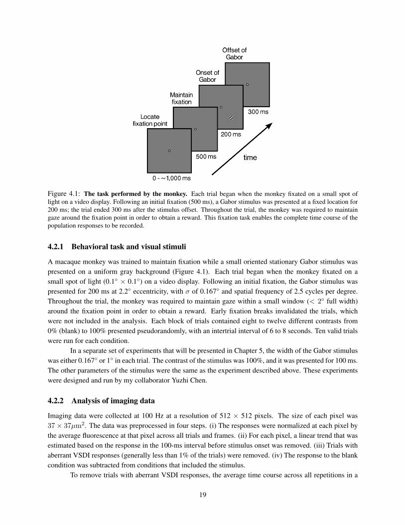
Figure 4.1: The task performed by the monkey. Each trial began when the monkey fixated on a small spot oflight on a video display. Following an initial fixation (500 ms), a Gabor stimulus was presented at a fixed location for200 ms; the trial ended 300 ms after the stimulus offset. Throughout the trial, the monkey was required to maintaingaze around the fixation point in order to obtain a reward. This fixation task enables the complete time course of thepopulation responses to be recorded.

4.2.1 Behavioral task and visual stimuli

A macaque monkey was trained to maintain fixation while a small oriented stationary Gabor stimulus waspresented on a uniform gray background (Figure 4.1). Each trial began when the monkey fixated on asmall spot of light (0.1◦ × 0.1◦) on a video display. Following an initial fixation, the Gabor stimulus waspresented for 200 ms at 2.2◦ eccentricity, with σ of 0.167◦ and spatial frequency of 2.5 cycles per degree.Throughout the trial, the monkey was required to maintain gaze within a small window (< 2◦ full width)around the fixation point in order to obtain a reward. Early fixation breaks invalidated the trials, whichwere not included in the analysis. Each block of trials contained eight to twelve different contrasts from0% (blank) to 100% presented pseudorandomly, with an intertrial interval of 6 to 8 seconds. Ten valid trialswere run for each condition.

In a separate set of experiments that will be presented in Chapter 5, the width of the Gabor stimuluswas either 0.167◦ or 1◦ in each trial. The contrast of the stimulus was 100%, and it was presented for 100 ms.The other parameters of the stimulus were the same as the experiment described above. These experimentswere designed and run by my collaborator Yuzhi Chen.

4.2.2 Analysis of imaging data

Imaging data were collected at 100 Hz at a resolution of 512 × 512 pixels. The size of each pixel was37 × 37µm2. The data was preprocessed in four steps. (i) The responses were normalized at each pixel bythe average fluorescence at that pixel across all trials and frames. (ii) For each pixel, a linear trend that wasestimated based on the response in the 100-ms interval before stimulus onset was removed. (iii) Trials withaberrant VSDI responses (generally less than 1% of the trials) were removed. (iv) The response to the blankcondition was subtracted from conditions that included the stimulus.

To remove trials with aberrant VSDI responses, the average time course across all repetitions in a

19

given condition was subtracted from the response in each trial, and the standard deviation of the residuals wascomputed at each frame. Trials with residual responses that were greater than three standard deviations wereexcluded from further analysis. This simple procedure eliminates trials where the animal made excessivemovements.

After the preprocessing, the spatial properties of the responses in individual trials were determined.First, the center of the spatial response of each experiment was estimated by fitting a two-dimensional (2D)Gaussian to the average response taken over a time window of 160 to 260 ms after stimulus onset (shadedregion in Figure 4.3a) for stimulus contrasts from 25% to 100%. This center was then held fixed, while theaverage response over the same time window was fitted with a 2D Gaussian to determine the lengths of themajor and minor axes and the orientation of the major axis for each trial in each condition of the experiment.

To include more trials at each contrast level in the analysis, a pooled dataset was formed by com-bining the responses of five experiments on one monkey. Due to the slight difference in the setup of eachexperiment, the spatial responses were translated and rotated with respect to each other. To align the data,the center and average orientation of the 2D Gaussian fit of each experiment were used to transform the dataso that the spatial responses aligned and overlapped in all the experiments. Data from individual experimentsare similar to the combined data.

4.3 Population responses to a Gabor stimulus in V1

In this section, the spatiotemporal properties of the VSDI responses measured in the experiments will becharacterized in detail. Since the VSDI responses in V1 are largely determined by the contrast of the Gaborstimulus, this dissertation focuses on the entire region in V1 that responds to the contrast envelope of thestimulus.

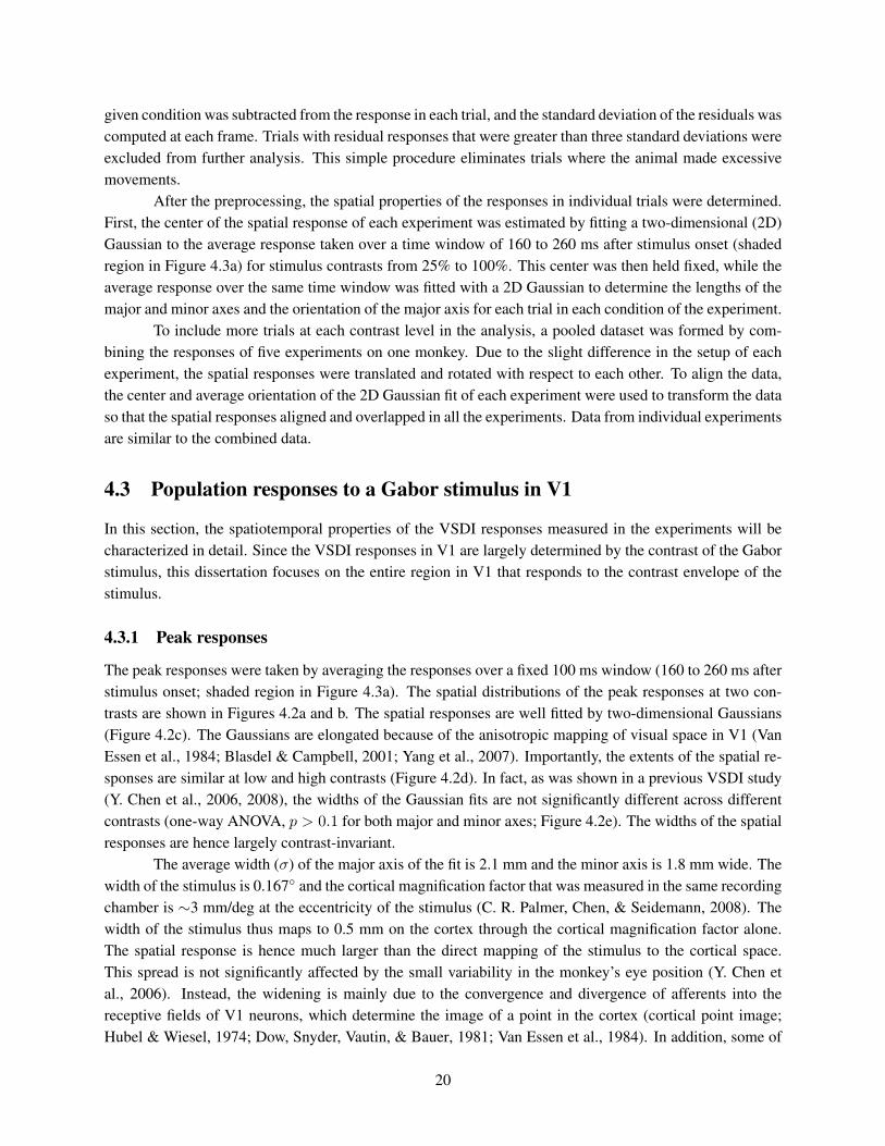
4.3.1 Peak responses

The peak responses were taken by averaging the responses over a fixed 100 ms window (160 to 260 ms afterstimulus onset; shaded region in Figure 4.3a). The spatial distributions of the peak responses at two con-trasts are shown in Figures 4.2a and b. The spatial responses are well fitted by two-dimensional Gaussians(Figure 4.2c). The Gaussians are elongated because of the anisotropic mapping of visual space in V1 (VanEssen et al., 1984; Blasdel & Campbell, 2001; Yang et al., 2007). Importantly, the extents of the spatial re-sponses are similar at low and high contrasts (Figure 4.2d). In fact, as was shown in a previous VSDI study(Y. Chen et al., 2006, 2008), the widths of the Gaussian fits are not significantly different across differentcontrasts (one-way ANOVA, p > 0.1 for both major and minor axes; Figure 4.2e). The widths of the spatialresponses are hence largely contrast-invariant.

The average width (σ) of the major axis of the fit is 2.1 mm and the minor axis is 1.8 mm wide. Thewidth of the stimulus is 0.167◦ and the cortical magnification factor that was measured in the same recordingchamber is ∼3 mm/deg at the eccentricity of the stimulus (C. R. Palmer, Chen, & Seidemann, 2008). Thewidth of the stimulus thus maps to 0.5 mm on the cortex through the cortical magnification factor alone.The spatial response is hence much larger than the direct mapping of the stimulus to the cortical space.This spread is not significantly affected by the small variability in the monkey’s eye position (Y. Chen etal., 2006). Instead, the widening is mainly due to the convergence and divergence of afferents into thereceptive fields of V1 neurons, which determine the image of a point in the cortex (cortical point image;Hubel & Wiesel, 1974; Dow, Snyder, Vautin, & Bauer, 1981; Van Essen et al., 1984). In addition, some of

20

(a) (b) (c)

(d) (e)

(f )

Figure 4.2: Peak responses to a Gabor stimulus. The responses were averaged across all experiments and overa fixed 100 ms time window (shaded region in Figure 4.3a). (a,b) Normalized peak responses to the stimulus at 6%(a) and 100% (b) contrasts in space. As expected from the anisotropy in the map of visual space in V1 (Van Essenet al., 1984; Blasdel & Campbell, 2001; Yang et al., 2007), the spatial profile is elongated along the axis parallel toV1/V2 border (white dashed line in (a)). (c) 2D Gaussian fit of the response in (b). The outlined regions representthe intersection between a 1.0 mm strip along the major axis and six concentric circular annuli of width 0.5 mm. Thecentral annulus is a disk with 0.5 mm radius. The responses of the pixels in the groups that are equidistant from thecenter are averaged for further analysis in Figures 4.3 to 4.7. (d) Normalized peak responses along the major axisat different stimulus contrasts. Error bars represent the standard errors across individual trials in all the figures. (e)The average widths of the Gaussian fits at different contrasts. The mean for the major axis is 2.1 mm and 1.8 mm forthe minor axis. (f) Contrast response function at the center. The solid curve is the Naka-Rushton equation fit to thedata (open circles, r2 = 0.98). The spatial profiles of the peak responses are therefore largely contrast-invariant, eventhough the responses saturate at high contrast, as was shown previously (Y. Chen et al., 2006, 2008).

21

this widening could reflect significant lateral spread of activity through lateral connections in V1 (Gilbert& Wiesel, 1979; Rockland & Lund, 1983; Martin & Whitteridge, 1984) and significant contribution fromfeedback connections (Angelucci, Levitt, & Lund, 2002; Angelucci, Levitt, Walton, et al., 2002).

Figure 4.2f shows the average peak response over a circular region of 0.5 mm radius at the centerof the response profile (central disk outlined in Figure 4.2c) as a function of stimulus contrast. Similarlyto single units, the responses follow a sigmoidal function on a log contrast axis; the solid curve is a Naka-Rushton function (Cn/(Cn50 + Cn); Naka & Rushton, 1966) fitted to the data (r2 = 0.98).

The peak response is a nonlinear function of contrast and saturates at about 25%. This result isinconsistent with models in which the response scales with input, such as the push-pull inhibition models(Troyer et al., 1998, 2002; Section 3.2.2) and some of the spatially organized leaky integrators (Ben-Yishaiet al., 1995; Somers et al., 1995; Hansel & Sompolinsky, 1998; Section 3.3.2). After saturation, the VSDIresponse does not decrease as contrast increases, which is inconsistent with the LIF models (Section 3.3.1).

4.3.2 Overview of the temporal response properties at different locations

To analyze the response properties at different locations in V1, the imaged pixels were divided into small binsaccording to their distances from the center of activity. The image was first divided into concentric annularregions 0.5 mm wide, centered at the peak of the spatial response, with the central region being a disk witha 0.5 mm radius. The pixels in the central region had an average distance of 0.25 mm from the center, andthis distance increased by 0.5 mm in each annulus. Due to the anisotropic response profile, pixels that are atthe same distance from the center can have different response amplitudes and potentially different temporaldynamics. Therefore, it is inappropriate to bin pixels according to distances alone. Instead, only the pixelswithin a 1 mm wide strip along the major axis of the fitted Gaussian profile were considered. Within thisstrip the relationship between distance and amplitude was nearly constant. The temporal responses of thepixels within each annulus that were also inside of the strip were averaged to produce a single time coursefor the corresponding distance. Figure 4.2c shows the bins up to an average distance of 2.75 mm. Responsesat locations further away were not analyzed because they were weak and noisy, especially at lower contrasts.

Figure 4.3a shows the average time courses of the responses at the center bin for different stimuluscontrasts. To characterize these time courses quantitatively, they were first divided into two parts. The firstpart, defined as the rising edge, was the response in the first 210 ms after the stimulus onset. The rest ofthe time course was defined as the falling edge. Each individual edge from each trial was smoothed by afive-frame moving average, normalized, and then fitted separately with a logistic function 1/(1 + eλ(t−t50))(e.g., Figure 4.3b). The parameter t50 is the time that the response reaches half of its peak, and λ describesthe slope of the response. For example, a λ of 0.05 means that the response takes about 44 ms after t50

to reach 90% of the peak. The same fitting procedure was applied independently at the different locationsshown in Figure 4.2c for each stimulus contrast. The latency of the rising edge (t10) was defined as the timeafter stimulus onset for the fitted response to reach 10% of its amplitude, where the change in slope is high.Similarly, the latency of a falling edge is defined as the time it takes for the response to decrease by 10%from the peak after stimulus offset.

Figure 4.3c shows the latencies of the rising and falling edges as a function of contrast in the centerbin. As observed in single neuron studies (Dean & Tolhurst, 1986; Carandini & Heeger, 1994; Albrecht,1995) and Figure 4.3b, the latency of the rising edge decreases as stimulus contrast increases (one-wayANOVA, p < 0.01). On the other hand, there is no significant difference in the falling edge latencies fordifferent contrasts (one-way ANOVA, p > 0.15). Asymmetric properties between rising and falling edges

22

(a) (b)

(c) (d)

Figure 4.3: Temporal responses to different stimulus contrasts at the center. (a) Time courses of the normalizedresponses in the center disk of Figure 4.2c. The stimulus was presented at time 0 and disappeared after 200 ms (dottedline). Average responses in the shaded area were used to compute the spatial profiles and contrast response function inFigure 4.2. (b) Logistic fits of the time courses in (a). The time courses were divided into two parts by the dotted lineat 210 ms. Each part was fitted separately by a logistic function. Diamond and square symbols on each part indicatethe latencies and times to half peak, respectively. Latencies (c) and slopes (d) of the rising and falling edges of thefitted responses as a function of contrast. While the shape of the rising edge depends on stimulus contrast, that of thefalling edge does not. Such asymmetry is a new observation and hence provides new constraints on models of V1.

are also observed in their slopes (Figure 4.3d). The slope of the rising edge becomes steeper as contrastincreases (one-way ANOVA, p < 0.01), while the falling edge slope remains similar (one-way ANOVA,p > 0.15). Such asymmetry is observed in all locations, as will be demonstrated next.

The space-time color plots in Figure 4.4 summarize in a compact form all of the temporal responsesas a function of stimulus contrast and position. The normalized fitted responses for each contrast are shownas separate subplots. Within each subplot the time course of the response at each of the six location binsfrom Figure 4.2c is indicated by a horizontal row, progressing from the center location at the top to themost peripheral location at the bottom. For example, the upper horizontal row in the space-time plot for100% contrast corresponds to the dark blue curve in Figure 4.3b. Several qualitative observations can bemade from these maps, which will be quantified in Sections 4.3.3 and 4.3.4. For each contrast, (1) theresponse latencies at different locations are approximately equal, as can be seen by the vertically aligned

23

Figure 4.4: Spatiotemporal responses to different stimulus contrasts. Logistic fits of the normalized time coursesat different locations for each stimulus contrast. Each horizontal row within the space-time plot for a given contrastshows the fitted time course at one location, from the center (top row) to the outmost region (bottom row). There is asystematic change in slope and latency of the rising edges, whereas the falling edges are similar for different contrastsand locations. This rich spatiotemporal response dynamics place strong constraints on models of V1.

transitions from blue to cyan in each map, and (2) the response rises at a slower rate as distance from thecenter increases, as can be seen by the tilt of the transition between colors as the normalized amplitudeincreases. In addition, for each location, as contrast increases (3) response latency decreases, and (4) theresponse rises at a faster rate. Finally, (5) after stimulus offset, the falling edges are similar for all locationsand contrasts. As will be shown in the next section, this rich spatiotemporal response dynamics place strongconstraints on models of V1.

4.3.3 Properties of the rising edge

The above observations can be demonstrated quantitatively using the logistic fits obtained from individ-ual trials. Figure 4.5a plots the rising edge latency (t10) as a function of distance from the center bin foreach stimulus contrast. There was no significant difference in the latencies at different locations (one-wayANOVA, p > 0.1 for all contrasts). On the other hand, as observed at the center bin, latency of the risingedge decreased as stimulus contrast increased at all locations (one-way ANOVA, p < 0.01 for all locations).These quantitative results confirm qualitative observations (1) and (3).

Figure 4.5b plots the same latency data in Figure 4.5a, but as a function of the peak response. For thesame response amplitude, the latency can be different at different stimulus contrasts. For example, responsesto a low-contrast stimulus at the center have much longer latency than the response 2.75 mm from the centerfor a high contrast stimulus even though the response amplitudes are the same. This result demonstrates thatthe dynamics of the response at a given location in V1 do not depend solely on the local response amplitude,but rather on the response amplitudes over a larger region.

The rate λ at which the response rises depends on both stimulus contrast and on cortical location(Figure 4.5c). For a particular contrast, the slopes at different locations are significantly different (one-way

24

(a) (b)

(c) (d)

(e) (f )

Figure 4.5: Temporal properties of the rising edge. Time shown is relative to stimulus onset. (a) Latencies ofthe responses at different cortical distances from the center. There was no significant difference in the latencies atdifferent locations (one-way ANOVA, p > 0.1 for all contrasts) while the latency of the rising edge decreased asstimulus contrast increased at all locations (one-way ANOVA, p < 0.01 for all locations). (b) The same data as in (a),but plotted as a function of the peak response. Slopes of the responses at different locations (c) and peak responses(d). Time to half of the peak response as a function of location (e) and peak response (f). Combining these results,for a particular contrast, the responses at different locations started to rise at about the same time, but the slopes wereshallower at locations that were further away from the center, increasing the times to half peak at these locations(one-way ANOVA, p < 0.01 for all contrasts).

25

ANOVA, p < 0.01 for all contrasts). The responses at locations that were further away from the centerincreased more slowly, confirming observation (2). In addition, at a fixed location, the slope of the risingedge increased with contrast (one-way ANOVA, p < 0.01 for all locations), quantifying observation (4).Furthermore, the slope also increased with peak response with a correlation coefficient of 0.94 (Figure 4.5d).

To summarize, combining the first four observations, for a particular contrast, the responses at dif-ferent locations started to rise at about the same time, but the slopes were shallower at locations that werefurther away from the center. Lowering the stimulus contrast increased the latencies of the rising edge anddecreased their slopes. The time courses of the responses are therefore different at different locations. Thisresult is inconsistent with the LN models that only consider the instantaneous inputs (Sections 3.2.1 and3.2.3), which predict that the response time courses is the same everywhere.

Traveling wave of activity and lateral propagation

Due to the decreasing slope as a function of location in the rising edge, the time to half of the peak response(t50) increased at locations peripheral to the center of activity. If it was employed as a measure of latency, awave of activity would appear to be originating from the center (Figure 4.4). The average difference of thetime to half peak between locations 0.25 mm and 2.75 mm away from the center was 6.2 ms. This differencecorresponds to a propagation speed of 0.4 mm/ms, which is at the higher end of the speed of propagationthrough lateral connections (0.1-0.4 mm/ms; Hirsch & Gilbert, 1991; Murakoshi et al., 1993; Grinvald etal., 1994; Nelson & Katz, 1995; Gonzalez-Burgos et al., 2000; Telfeian & Connors, 2003).

As discussed in Section 3.2.4, if the difference in t50 is solely due to the slow lateral spread, thenbeyond a certain critical distance the response latency should increase linearly as a function of distance fromthe center. However, there was no significant difference in the rising edge latency of the VSDI responsesfor a wide range of distances (Figure 3a). In fact, for 50% and 100% contrast stimuli, rising edge latenciesremained the same up to a distance of 3.25 mm (within which a reasonably good fit to the data could beobtained; data not shown).

To investigate how the latencies are affected by lateral propagation in the proximity of the center, alinear model was simulated. The stimulus-driven signal in each model unit was assumed to have the samesigmoidal time course A(t), with amplitude c(x) proportional to the local contrast in the unit’s receptivefield. These stimulus-driven signals were propagated through lateral connections at a constant speed, whichwas implemented as a spatiotemporal kernel Gl(x, t):

Gl(x, t) =

{G(x) if t = |x−c|

v

0 otherwise,(4.1)

where v is the conduction speed, c is the center of the kernel, and G(x) is the weighting function of lateralconnections. The membrane potential of the unit were the sum of stimulus-driven signals and the incominglateral signals multiplied by a scaling factor w: c(x)A(t) + w (c(x)A(t)) ⊗ Gl(x, t), where ⊗ denotesconvolution.

In such a model, the overall strength, extent, and conduction speed of the lateral connections allcontribute to the time course of the membrane potential. In the simulation, the spatial strength of the lateralconnection G(x) and the receptive field envelope were assumed to follow a Gaussian profile. The widthsof the lateral connections σlat and the receptive field σrf were therefore constrained by the equation: σ2 =√σ2

stim + σ2rf + σ2

lat, where σ = 2.1 mm is the width of the response profile and σstim = 0.5 mm is the widthof the stimulus used in the experiment. For each scaling factor w and for each plausible pair of values of σrf

26

(a) (b)

Figure 4.6: Effects of lateral propagation on the latency of the rising edge. (a) The difference in latencies betweenthe locations that were 0.25 mm and 2.75 mm away from the center is plotted as a function of the ratio between thewidths of the receptive field and lateral connections for different values of the lateral weight scaling factor w. Eachcurve is plotted for the range where a fit to the time to half peak was possible. Shaded region shows the 95% confidenceinterval (truncated at 0) between the latencies at the two locations in the VSDI responses. (b) The increase in latency(top) and time to half peak (bottom) as a function of distance from the center for the three example points indicatedby different symbols in (a). These results show that in order to account for the traveling wave of activity with slowlateral connections, the latency of the rising edges has to be different at different locations, which is inconsistent withthe VSDI responses.

and σlat, the conduction speed v of the lateral connections was fitted such that the times to half of the peakresponse at distances 0.25 mm and 2.75 mm differed by 6.2 ms. The latencies (t10) at these two locationswere then determined from the fitted responses.

Figure 4.6a plots the latency difference as a function of the ratio between σrf and σlat for differentweights w over the range where a fit was possible. The difference in latencies is substantial. As the ratiobetween σrf and σlat increased, the fitted conduction speed decreased to compensate for the wider feedfor-ward receptive field. At the end of each curve in Figure 4.6a, the speed was less than 0.01 mm/ms, whichis an order of magnitude slower than the speed observed in lateral connections and may not be biologicallyplausible. For the values of the weight w that were tested, the predicted differences were larger than the 95%confidence interval of the latency difference in the VSDI responses. This result suggests that linear sum-mation of the delayed signals from lateral connections alone cannot account for the properties of the VSDIresponses consistently. Figure 4.6b plots how the latency and time to half peak increase as a function ofdistance from the center for the two extreme points with w = 1 in Figure 4.6a (circle and triangle symbols)and the rightmost point for w = 0.01 (square symbol). Changing the shape of the stimulus-driven responsedid not affect these results, as long as it remained sigmoid.

Models with slow propagation of activity therefore do not satisfy with all the anatomical and phys-iological constraints. However, as will be discussed in the next chapter, such differences in time to halfof the peak and other properties can be explained by the population gain control model proposed in thisdissertation.

27

4.3.4 Properties of the falling edge

The dynamics of the falling edge of the responses were markedly different from those of the rising edge. Asshown in Figure 4.7, both latency and slope were independent of contrast and location (two-way ANOVA,p > 0.15 across contrasts and locations for both latency and slope). The responses at all locations there-fore fell approximately all at once and at the same rate, regardless of the stimulus contrast and responseamplitude, supporting observation (5).

The latency of the falling edge (t10 = 65 ms) was slightly larger than that of the rising edge atlow stimulus contrasts. As contrast increased, the rising edge accelerated, resulting in a shorter latencyand steeper slope, while the properties of the falling edge remained the same. The average slope for thefalling edge (λ = 0.026) was shallower than any slope of the rising edge. Such asymmetry in the temporalproperties of the rising and falling edges can be explained by the population gain control model presentedin the next chapter.

4.4 Discussion

Because VSDI measures changes in membrane potentials in a small volume of V1, it is unclear how theVSDI signals relate to the population responses at the level of spiking activity: For instance, they mayhave different spatiotemporal dynamics. A recent quantitative comparison of VSDI and extracellular mi-croelectrode recordings in V1 of fixating monkeys showed that the relationship between the normalizedVSDI responses and spiking activities of small neural populations is nonlinear and can be approximated bya power function (C. R. Palmer et al., 2008). Because a power function of a Gaussian is also a Gaussianbut of a different width, and because the spatial profile of the VSDI responses to a small Gabor stimulus isa Gaussian, the spatial profile of the population spiking activities may also be independent of contrast forsuch stimuli. Further experimental investigations are required to address this and other similar questionsconcerning the relationship between VSDI signals and spiking activity of a neural population.

Functionally, the power function implements a soft threshold for spiking activity: The normalizedVSDI response has to be large enough for the spiking activity to be noticeable. In fact, C. R. Palmer etal. (2008) observed no significant spiking activity in V1 when the normalized VSDI response was below0.3. Such a threshold can explain some of the discrepancies between the behaviors of single unit and VSDIresponses. For example, while the falling edge latency is larger than the rising edge for all contrasts in theVSDI response, the reverse relationship is observed in the firing rates of single units (Bair et al., 2002). Theapparent discrepancy is consistent with the fact that the VSDI measures subthreshold membrane potentials(Grinvald et al., 1994). Because of spike threshold, the onset of spiking activity will lag behind the rise inthe VSDI response. On the other hand, for the falling edge the drop in spiking activity will coincide with thedrop in the VSDI response (as long as membrane potential is above threshold). Thus, for spikes it is quitepossible for the onset latency to be greater than the offset latency.

4.5 Conclusion

To understand the processing of arbitrary visual stimuli in the cortex, it is important to characterize theproperties of V1 population responses. This chapter provides the first quantitative description of the real-time spatiotemporal dynamics of V1 population responses to brief, localized visual stimuli. The population

28

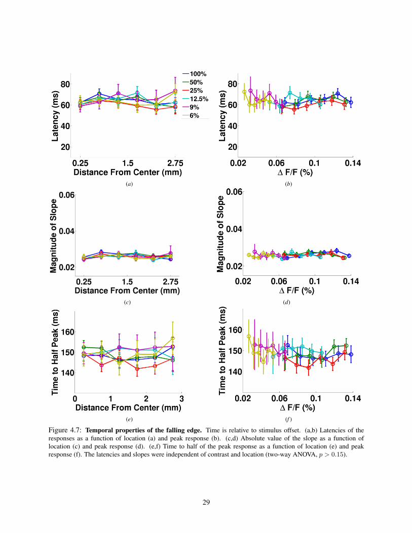
(a) (b)

(c) (d)

(e) (f )

Figure 4.7: Temporal properties of the falling edge. Time is relative to stimulus offset. (a,b) Latencies of theresponses as a function of location (a) and peak response (b). (c,d) Absolute value of the slope as a function oflocation (c) and peak response (d). (e,f) Time to half of the peak response as a function of location (e) and peakresponse (f). The latencies and slopes were independent of contrast and location (two-way ANOVA, p > 0.15).

29

responses exhibit systematic and unexpected nonlinear properties that are not obvious from single unit re-sponses. First, the spatial profile of the response is constant and independent of stimulus contrast. Second,responses start to rise at all locations simultaneously, but rise at a faster rate at the center of activity than atperipheral locations. Third, both the latency and the steepness of the rising edge of the response depend onstimulus contrast. Finally, after stimulus offset, the responses at all locations fall simultaneously and at thesame rate, regardless of stimulus contrast. These results illustrate that unexpected properties can emerge atthe level of neural population responses (Seidemann, Chen, & Geisler, 2009). In general, it will be difficultor even impossible to predict the population responses based on a small sample of single-unit measurementsin many cases. These unexpected properties demonstrate that it is important to characterize populationresponses quantitatively in both space and time.

The properties of the VSDI responses, such as response saturation and contrast-dependent slope ofthe rising edge, are inconsistent with the LN and LIF models for single neurons and spatially organizednetworks. On the other hand, the NGC models have been shown to account for such properties in singleneurons (Albrecht & Geisler, 1991; Heeger, 1992; Carandini & Heeger, 1994; Carandini et al., 1997; Manteet al., 2008). Thus, normalization models are more promising than the other families of models. However,an important question is whether normalization models can account for the other properties observed in theVSDI data, especially the changes in the rising edge at different locations and the invariance of the slopeand latency of the falling edge. In the next chapter, a more general form of normalization model calledpopulation gain control (PGC) model that can account for all the spatiotemporal properties of the VSDIresponses will be presented.

30

Chapter 5

Population Gain Control Model

Normalization gain control models have been used to account for many nonlinear properties of single unitresponses in the LGN and V1 (Albrecht & Geisler, 1991; Heeger, 1992; Carandini et al., 1997; Mante et al.,2008). In particular, this family of models can explain response saturation (Albrecht & Hamilton, 1982),contrast-invariant tuning (Skottun et al., 1987; Albrecht & Geisler, 1991; Sclar & Freeman, 1982), and phaseadvance of response at high stimulus contrasts (Carandini et al., 1997). As shown in the previous chapter,these properties are also observed in the V1 population responses. Thus, normalization models are morepromising than other families of models. However, an important question is whether normalization modelscan account for the other properties observed in the VSDI data, such as the changes in the rising edge atdifferent locations and the invariance of the slope and latency of the falling edge. In this chapter, a moregeneral form of normalization model called population gain control model (Sit, Chen, Geisler, Seidemann,& Miikkulainen, 2008) is defined. This model can account for most of the spatiotemporal properties of theVSDI responses, suggesting that population gain control is a general mechanism of visual processing.

5.1 Population gain control (PGC) model

The population gain control (PGC) model is a generalization of the normalization models (Albrecht &Geisler, 1991; Heeger, 1992; Carandini et al., 1997; Mante et al., 2008). In contrast to traditional gaincontrol models, which apply to the temporal dynamics of a single neuron, the PGC model aims at explainingthe responses of a large neural population in both time and space.

In the model, the early visual pathway is represented by a network consisting of an input sheet andtwo stages (Figure 5.1a). The input sheet represents the visual stimulus and does not perform any processing.The first stage in the model represents the nonlinear processing that occurs in the retina, LGN, and layer4 in V1. While it would be more realistic to model each of these areas individually, there is not enoughexperimental data at the population level to provide sufficient constraints to do so. The second stage modelsthe superficial layers in V1 from which the VSDI signals are measured. Within each stage, the units areidentical and implement the filtering and normalization circuit illustrated in Figure 5.1b.

To simplify the discussion and simulation, each of these sheets are represented by a one-dimensionalarray, which represents the collapsed data along the major axis (x-axis) of the VSDI response profile (theblack rectangular region in Figure 4.2c). Each sheet thus contains an array of units indexed by x, whereeach unit represents the average activity of the small neural population within a pixel in the VSDI image.Extension to two dimensions is straightforward mathematically and results in similar response properties.

31

(a) (b)

(c)

Figure 5.1: A canonical model of visual processing. (a) A feedforward gain control model for the early visualpathway. The model consists of an input sheet and two stages. Each sheet is modeled by a spatially organized arrayof units with the same set of parameters. The input sheet represents the visual stimulus only and does not employthe model in (b). The processing in the first stage represents the nonlinearity in the retina, LGN, and layer 4 of V1,whose spiking responses are fed into the second stage as input. The second stage represents the superficial layers inV1 from which the VSDI signals are measured. The blue and red projections illustrate the receptive fields R(x) andnormalization poolsN(x), respectively, for two example units in the first (light colors) and second (dark colors) stagesof the model. (b) The processing in a model unit. Each unit computes two weighted sums: A(x, t) from the receptivefield, and B(x, t) from normalization pool. A(x, t) is the driving current of the parallel resistor-capacitor (RC) circuitthat represents the processing at each pixel of VSDI imaging. The conductance g(x, t) of the resistor is controlledby the normalization activity B(x, t) and is inversely related to the gain of the circuit, i.e. it has a divisive effect onthe sum A(x, t). It also affects the dynamics of the response. The voltage across the capacitor is the unit’s response.(Figure modified from Carandini et al., 1997.) (c) Example time courses of the model’s components at the center andperiphery of a hypothetical stimulus.

32

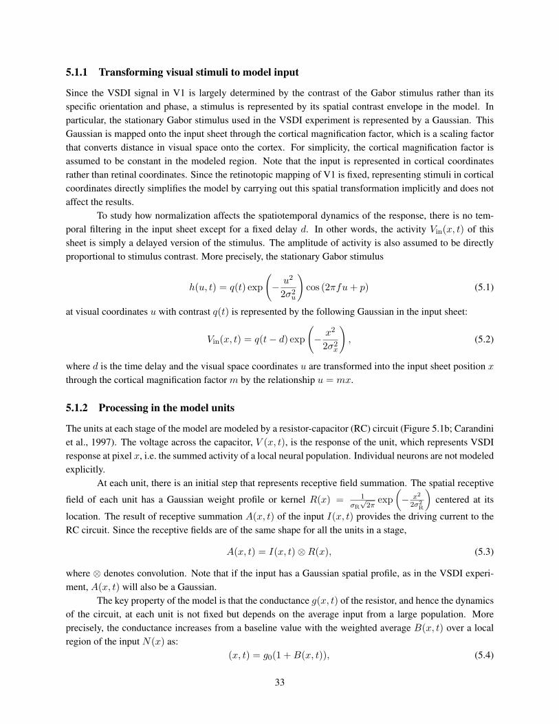
5.1.1 Transforming visual stimuli to model input

Since the VSDI signal in V1 is largely determined by the contrast of the Gabor stimulus rather than itsspecific orientation and phase, a stimulus is represented by its spatial contrast envelope in the model. Inparticular, the stationary Gabor stimulus used in the VSDI experiment is represented by a Gaussian. ThisGaussian is mapped onto the input sheet through the cortical magnification factor, which is a scaling factorthat converts distance in visual space onto the cortex. For simplicity, the cortical magnification factor isassumed to be constant in the modeled region. Note that the input is represented in cortical coordinatesrather than retinal coordinates. Since the retinotopic mapping of V1 is fixed, representing stimuli in corticalcoordinates directly simplifies the model by carrying out this spatial transformation implicitly and does notaffect the results.

To study how normalization affects the spatiotemporal dynamics of the response, there is no tem-poral filtering in the input sheet except for a fixed delay d. In other words, the activity Vin(x, t) of thissheet is simply a delayed version of the stimulus. The amplitude of activity is also assumed to be directlyproportional to stimulus contrast. More precisely, the stationary Gabor stimulus

h(u, t) = q(t) exp

(− u2

2σ2u

)cos (2πfu+ p) (5.1)

at visual coordinates u with contrast q(t) is represented by the following Gaussian in the input sheet:

Vin(x, t) = q(t− d) exp

(− x2

2σ2x

), (5.2)

where d is the time delay and the visual space coordinates u are transformed into the input sheet position xthrough the cortical magnification factor m by the relationship u = mx.

5.1.2 Processing in the model units

The units at each stage of the model are modeled by a resistor-capacitor (RC) circuit (Figure 5.1b; Carandiniet al., 1997). The voltage across the capacitor, V (x, t), is the response of the unit, which represents VSDIresponse at pixel x, i.e. the summed activity of a local neural population. Individual neurons are not modeledexplicitly.

At each unit, there is an initial step that represents receptive field summation. The spatial receptive

field of each unit has a Gaussian weight profile or kernel R(x) = 1σR

√2π

exp(− x2

2σ2R

)centered at its

location. The result of receptive summation A(x, t) of the input I(x, t) provides the driving current to theRC circuit. Since the receptive fields are of the same shape for all the units in a stage,

A(x, t) = I(x, t)⊗R(x), (5.3)

where ⊗ denotes convolution. Note that if the input has a Gaussian spatial profile, as in the VSDI experi-ment, A(x, t) will also be a Gaussian.

The key property of the model is that the conductance g(x, t) of the resistor, and hence the dynamicsof the circuit, at each unit is not fixed but depends on the average input from a large population. Moreprecisely, the conductance increases from a baseline value with the weighted average B(x, t) over a localregion of the input N(x) as:

(x, t) = g0(1 +B(x, t)), (5.4)

33

where g0 is the baseline conductance and B(x, t) = k · I(x, t)⊗N(x). For reasons that will become clearin the next section, N(x) is called the normalization pool and B(x, t) the normalization activity. The spatialnormalization poolN(x) is assumed to have a Gaussian weight profileN(x) centered at the location of eachunit. It is assumed to be wider than the receptive field, i.e. σN > σR, so that a larger region contributes tothe conductance rather than just the area within the receptive field. The multiplicative factor k controls theoverall strength of normalization.

The membrane potential V (x, t) can then be described by the RC circuit equation

C∂V (x, t)∂t

= A(x, t)− g(x, t)V (x, t), (5.5)

where C is the constant membrane capacitance.

5.1.3 General behavior of a model stage

One way to illustrate the dynamics of a stage in the model is through a step input that was used in the VSDIexperiment:

I(x, t) =

{J(x), 0 ≤ t ≤ tf0 otherwise,

(5.6)

where J(x) is a Gaussian that models the Gabor stimulus and tf is the time when the stimulus disappears.During the stimulus presentation, both the driving current A and the conductance g0(1 + B) are constant(Figure 5.1c), and the dynamics of the model simplifies to

C∂V (x, t)∂t

= A(x)− g0(1 +B(x)) V (x, t), (5.7)

which has the solution:

V (x, t) =A(x)

g0(1 +B(x))

(1− exp

(−g0(1 +B(x))

Ct

)). (5.8)

Equation 5.8 above simply describes the process of charging a capacitor with time constant Cg0(1+B(x)) =

Cg(x) , i.e. the conductance and the time constant are inversely related.

Rising edge of the response

The key property of the model is that conductance g(x, t) depends on the average input from a large popu-lation. When normalization activity B(x, t) at a unit is high, conductance is large and the time constant issmall. Thus, when normalization activity is high the response can change rapidly to a change in the input.This property can account for much of the dynamics observed in the VSDI responses. At a particular unit,when the stimulus contrast is high, the input amplitude and hence the normalization activity is large, result-ing in faster dynamics (Figure 5.1c). This property is consistent with the observed dynamics in the risingedge of the VSDI responses at a particular location for different contrasts.

For a Gabor stimulus, the normalization activity is largest at the center, where contrast is the highest(Figure 5.1c). The response at the center therefore rises at a faster rate than that at the periphery, whichagain is consistent with the observed properties of VSDI responses. This is an interesting property becausethe spatial difference in time constants can account for the traveling wave observed at the rising edge evenwithout slow lateral connections that are generally hypothesized to be the cause of the wave (Hirsch &Gilbert, 1991; Murakoshi et al., 1993; Grinvald et al., 1994; Nelson & Katz, 1995; Gonzalez-Burgos et al.,2000; Telfeian & Connors, 2003).

34

Steady state response

When the stimulus is presented long enough, the membrane potential will reach a steady state V (x) =A(x)

g0(1+B(x)) = A(x)g(x) . In other words, the gain of the circuit is the inverse of conductance, and therefore

the conductance has a divisive (normalizing) effect on the output of the receptive field summation. Sinceconductance is a function ofB(x, t),B(x, t) is called the normalization activity and the weight profileN(x)is called the normalization pool. The overall strength of normalization is controlled by the multiplicativefactor k that scales B(x, t). Note that, as indicated in Figure 5.1c, the conductance is set instantly by thecurrent value of the normalization pool without any additional time lag or temporal filtering. One way thisprocess might be implemented biologically would be with feedforward inhibition, as reviewed in Chapter 2,that is as rapid or more rapid than the excitation.

To analyze how the steady-state response changes with contrast for the stimuli used in the VSDIexperiment, note that for a given unit x, B(x) can be written as r(x)A(x). This gives the steady-stateresponse

Vs(x) =A(x)

g0(1 + r(x)A(x)), (5.9)

which is a saturating function of A(x) that approaches 1/(g0r(x)) as A(x) increases. Such saturation isdesirable for modeling the contrast response observed in experiments.

Falling edge of the response

When the stimulus disappears at tf , bothA andB become zero. This effect leads to the following dynamics:

C∂V (x, t)∂t

= −g0V (x, t), (5.10)

which has a simple solution:V (x, t) = V0(x)e−

g0C

(t−tf ), (5.11)

where V0(x) is the response at the time of stimulus offset tf . This solution has three important implications.First, the responses at all locations start to decay all at once after the stimulus disappears, regardless ofstimulus contrast and V0. Second, the responses decay with the same time constant C/g0 at all locations(Figure 5.1c). Finally, note that the time constant of the rising edge C/(g0(1+B(x))) is smaller than C/g0.This observation explains why the slopes of the falling edges are shallower than those in the rising edges inthe data. The dynamic nonlinearity in the model therefore can account for many of the observed propertiesof the population responses.

More general input time course

With the stimuli used in the VSDI experiments, the above analysis of the model’s dynamics is exact for thefirst stage because the time course of the stimulus is a step function. However, in general, the input takestime to build up and fall off. This is the case in particular for the second stage where the input is the responseof the first stage. The solution for the membrane voltage V (x, t) will therefore have a more complex form.

Although in general there is no analytical solution to V (x, t) for arbitrary input time course, forthe stimulus used in the VSDI experiments the three phases of the responses in the second stage can bequalitatively analyzed. Because the spatial profile of the input is unimodal, the normalization activity inthe second stage is the largest at the center of the stimulus and with large input amplitude. The rising edge

35

of the response is therefore fast in these conditions, as it is for a step input. Such unimodal distribution ofnormalization activity also exists during the falling edge in the second stage because its input, i.e. response inthe first stage, decays exponentially at all locations instead of turning off instantly. However, the differencebetween the falling edges at different locations will be smaller than that of the rising edges because (1)the input falls at the same rate for all locations, whereas there is already a difference in the rising edgesof the input, and (2) the responses will all decay at same rate when the input becomes negligible. Finally,the steady-state response in the second stage will also saturate at high input, by the same argument as inSection 5.1.3. As will be shown in Section 5.4.1, the dynamics of the responses in the second stage thusremain similar to those for a step input and are consistent with the observed population responses in V1.

5.1.4 Response transformation between stages

The response V (x) at pixel x in the model represents membrane potential, which dominates the VSDIresponses. Since neurons communicate through spikes, the responses in the first stage have to be convertedinto spikes that the second stage receives. As mentioned in Section 4.4, a recent study showed that the VSDIresponses can be related to spiking activities by a power function (C. R. Palmer et al., 2008). A similarrelationship has also been found between the average membrane potential and the firing rate in single unitrecordings (Anderson, Lampl, Gillespie, & Ferster, 2000; Finn, Priebe, & Ferster, 2007). A fixed powerfunction is thus applied to the responses in the first stage and the results are fed into the second stage asinputs:

I2(x, t) = V1(x, t)n, (5.12)

where the subscripts denotes the stages.While the stimulus represented in the input sheet can be fed directly to the first stage to provide

a reasonably good fit to the data, the predictions shown in this dissertation are for a model with a secondfixed power function applied to the activity in the input sheet. This initial nonlinearity is plausible given theaccelerating point nonlinearities seen in the earliest levels of the visual system; e.g. the nonlinear relation-ship between the membrane potential of the photoreceptors and their rate of glutamate release (Witkovsky,Schmitz, Akopian, Krizaj, & Tranchina, 1997) that excites the downstream neurons in the retina.

While the power function accelerates both rising and falling edges, it preserves the relationshipbetween speed and amplitude of responses among different locations. In particular, the falling edge of theresponse in the first stage still falls at the same rate at all locations: (e−

tτ )n = e

− tτ/n . The Gaussian profile

in the input sheet is also preserved: (exp(−x2

σ2 ))n = exp(− x2

σ2/n). Thus the analytical results presented in

this section still apply.

5.2 Effects of normalization pool size

When a step input is presented, the response at each model unit rises with a time constant that dependson its conductance. Since conductance is a function of normalization activity, it in turn depends on twofactors in the model: (1) the multiplicative factor k that scales it, and (2) the spatial weighting functionof the normalization pool N(x). The width of the weighting function is important biologically because itrepresents the size of the pool of neurons that contributes to the response dynamics at one location. Thissection discusses how it affects the rising edge and the spatial profile of the response.

36

Consider a fixed localized input and different Gaussian normalization weighting functions that havethe same total weight. If the pool is wide, then the normalization activity will be similar for units near andfar from the center of activity. Thus, the difference in the slopes of the rising edges across space will besmall. On the other hand, if the normalization pool is small, there will be a large difference in the timeconstants of different units. Varying the size of the pool thus changes the time courses of the rising-edgeresponses at different locations. These considerations suggest that the observed difference between the timecourses at the different locations can be explained by a feedforward PGC model with an appropriate poolsize.

Normalization pool size also influences the spatial profile of the response. Consider a static Gaussianinput and its corresponding steady-state response, V (x) = A(x)/g(x). If the pool is much wider than theinput, then the normalization activity and hence the conductance g(x) will be the same at all units. In thiscase, the spatial response profile will simply be a scaled version of the receptive field summation, thuspreserving the shape of A(x). On the other hand, if the normalization pool is much narrower than the input,then response saturation will occur at a different stimulus contrast for each unit as in the LN model, thusflattening the response profile at high contrasts. As a result, to achieve the contrast-invariant spatial profileobserved in the VSDI responses, the normalization pool size has to be at least comparable to the size of thestimulus used.

In summary, the normalization pool size affects both spatial and temporal properties of the responses.Based on these properties, it is possible to estimate the overall pool size and the other parameters from thedata of the VSDI experiment. The procedure is described in the next section.

5.3 Parameter estimation

The values of the parameters were estimated by fitting the responses in the second stage of the model to theVSDI responses. To reduce the number of free parameters, g0 is assumed to be 1.0 for both stages becauseit is effectively a scaling factor of the response and the conductance. The constant delay in the input sheetwas chosen to be 20 ms, which was a few milliseconds shorter than the shortest latency seen in the data. Theexponent of the power function that converts membrane potential into spikes was chosen to be 2.0, whichis similar to what has been found experimentally (C. R. Palmer et al., 2008) and provides a good fit to thedata. The same exponent is also used for the input sheet response.

Based on the literature suggesting that the widths of the center and surround in the afferents of V1are about half of those in V1 (Sceniak, Chatterjee, & Callaway, 2006), σR,2 = 2σR,1 and σN,2 = 2σN,1,where the number in the subscripts denote the stage of the model. Furthermore, the width (σ) of the VSDIspatial profile is assumed to be the result of cascaded receptive field summation and the power function. Thevalue of σR,1 is hence given by

σ2 = (σ2x/2 + σ2

R,1)/2 + σ2R,2 (5.13)

= (σ2x/4 + 9σ2

R,1)/2, (5.14)

where σx is the width of the stimulus in the input sheet.Using the measured rising edge time constants τc at the center location c and τp at the periphery

that is p mm from the center, the size of the normalization pool in the second stage σR,2 of the model canbe estimated. The procedure gives the lower bound for σR,2, because it does not take the difference in the

37

slopes of the input to the second stage into account; if there is already some difference in the input, σR,2

would need to be larger to offset the difference.From Section 5.1.3, τc is related to B(c):

τc =C

g0(1 +B(c))(5.15)

B(c) =τ

τc− 1, (5.16)

where τ = C/g0, which is the time constant of the falling edge. Since both τ and τc can be measured fromthe data, B(c) can be evaluated to give a numerical value. Similarly, B(p) = τ

τp− 1 and can be computed.

Note that B(x) is a Gaussian with width√σ2

1 + σ2N,2, where σ2

1 = (σ2x/2 + σ2

R,1)/2, and B(c) andB(p) are the values at their corresponding points. By dividing B(c) by B(p), the width of the normalizationpool in the second stage, σN,2, can be estimated:

B(c)B(p)

=1

exp(− p2

2(σ21+σ2

N,2)

) (5.17)

σ21 + σ2

N,2 =p2

2 ln(B(c)B(p)

) (5.18)

σN,2 =

√√√√ p2

2 ln(B(c)B(p)

) − σ21. (5.19)

The remaining free parameters that need to be estimated are C1, C2, k1, and k2. First, the steady-state contrast response function of the model is fitted to the data by minimizing the sum of the squared error.This step enabled k1 and k2 to be determined separately from C1 and C2, because the capacitances do notaffect the steady-state response of the model. After that, the normalization strengths, k1 and k2, were heldfixed, while the capacitances were estimated by fitting the slopes of the rising and falling edges at differentlocations and stimulus contrasts simultaneously.

5.4 Simulation of VSDI responses

The values of the parameters obtained in the above procedure were σR,1 = 0.983 mm, σN,1 = 1.386 mm,C1 = 3.19, C2 = 2.3, k1 = 1520, and k2 = 2. The cortical magnification factor measured in this chamberis about 3mm/deg (C. R. Palmer et al., 2008). With this set of parameters, the model was simulated for a 20mm long strip (extending the black rectangular region in Figure 4.2c) using the Matlab function ode45().

5.4.1 Results of the simulation

Figure 5.2a plots the spatial profiles of the peak responses in the second stage of the model for differentinput contrasts. Consistent with the VSDI responses, the widths of the profiles are all the same (Figure 4.2and Y. Chen et al., 2006, 2008). Note that profiles will only be contrast-invariant in the model for stimuliwith sizes that are smaller or comparable to the receptive field of the V1 units; due to saturation, profiles forlarge stimuli will change shapes and widths as a function of contrast. The contrast response function of themodel is plotted in Figure 5.2b, which provides a good fit to the data (r2 = 0.98).

38

(a) (b)

Figure 5.2: Peak responses of the second stage in the model. (a) Normalized spatial profile of the peak responses.The widths of the profiles are the same for different contrasts, which is consistent with the VSDI responses (Y. Chenet al., 2006, 2008). (b) Normalized contrast response function at the center. Circles are the responses from the data(Figure 4.2e). The quality of fit is high (r2 = 0.98). The model therefore captures the essential properties of the peakresponses observed in the data.

Figure 5.3 shows the space-time plot of the responses of the second stage in the model for differentcontrasts, using the same format as Figure 4.4. The model captures qualitatively the observed spatiotemporalproperties of the responses. For each contrast, (1) the rising edge latencies (t10) at different locations aresimilar, with a maximum difference of 2 ms, and (2) the slope of the rising edge becomes shallower asdistance from the center increases. For each location, as contrast increases, (3) response latency decreases,and (4) the rising edge becomes steeper. Finally, for all contrasts and locations, (5) latencies and slopesof the falling edges are similar (< 2 ms difference). Although there are some minor discrepancies at lowcontrast, e.g. the difference in the slopes of the rising edges across locations is smaller than the data, it isremarkable that such a simple model can account for most of the properties of the population responses inboth time and space.

5.5 Relative normalization strengths in the different stages

In the PGC model, normalization (contrast gain control) operates in the retina, LGN and in V1, as it doesin the primate visual system. There are many nonlinear properties of single unit responses in the retinaand LGN, such as phase advance of response at high contrast (Shapley & Victor, 1978; Victor, 1987),contrast saturation (Bonin et al., 2005), and size tuning (Bonin et al., 2005; Sceniak et al., 2006), that canbe explained by gain control. These nonlinearities are also observed in V1. It is therefore possible that gaincontrol before V1 contributes significantly to the response nonlinearities in V1. The main question is whatthe relative strength of the normalization in the different stages of visual processing is. It is an open andimportant question that is difficult to answer directly by empirical experiments.

This question can be addressed using the PGC model by considering the parameters k1 and k2 thatset the normalization strengths, and hence the degrees of nonlinearity, in the two stages of the model. Asit turns out, the stimuli used in the VSDI experiment are not sufficient to discriminate between hypotheses

39

Figure 5.3: Spatiotemporal responses of second stage in the model. The properties of the responses are similar tothe observed data shown in Figure 4.4, suggesting that population gain control may be a general mechanism of visualprocessing.

concerning relative normalization strength. However, by varying the size of the stimulus it is possible toestimate the relative contributions of normalization in the first stage (retina to layer 4 of V1) and the secondstage (superficial layers of V1): The relative strength of the normalization in the two stages has a largeimpact on the expected size tuning of V1 responses. Figure 5.4 shows the predicted response amplitude atthe center of the activated region in the superficial layers of V1 as a function of stimulus size. The contrastof the Gabor stimulus is 100%. Each curve in the figure is for a different strength of normalization in thefirst stage relative to the total strength in both stages of the model, i.e. k1/(k1 + k2). The curves havebeen scaled so that response is 1.0 for the Gabor size used in the VSDI experiment (σ = 0.167◦). Whennormalization only occurs in the first stage of the model (100%), the response increases with stimulus sizebecause the second stage is linear (i.e. no normalization). As the normalization in the second stage becomesstronger (the other curves), the relative response to the larger stimuli, e.g. σ = 1◦, decreases, becausenormalization has a divisive effect on the input from the first stage. For the parameter values that can fit theVSDI responses, further decrease of the relative normalization weakens size tuning.

In an additional biological experiment, the VSDI responses to 100% contrast Gabor stimuli withσ = 0.167◦ and 1◦ were measured. The red dots in Figure 5.4 plot the relative responses to the two stimuli.The peak response to the large stimulus is about 7% less than that of the small stimulus, which is consistentwith a strong (99%) normalization in the first stage of the model. This pair of normalization strengths wasused to obtain the simulation results shown in Figure 5.2 and 5.3.

This surprising result suggests that the nonlinearity observed in the data may be mostly implementedbefore the superficial layers of V1 where the VSDI signals are measured. It illustrates nicely how computa-tional model can be used not only to replicate the behavior of the responses, but to gain new insight aboutvisual processing.

40

Figure 5.4: Predictions of the size tuning curves of five example combinations of normalization strengths. Eachcurve represents a different combination of normalization strengths, labeled by the proportion of normalization in thefirst stage (k1/(k1 + k2)). The contrast of the stimulus is 100% and the response is measured at the center. The reddots plot the normalized responses obtained in the VSDI experiment for two stimulus sizes. The reduction of VSDIresponse to the large stimulus is small, which is consistent with a strong normalization in the first stage of the model.

5.6 Discussion

The complex spatiotemporal dynamics of the population responses in V1 can be captured by a simple PGCmodel. At the core of this model is divisive population gain control. Although it is a functional model ratherthan a detailed low-level biophysical model, the necessary neural substrate should exist to support such amechanism. In this section, issues of modeling population responses and possible biological implementationof divisive population gain control are discussed. The new insights that the PGC model provides, combinedwith quantitative analysis of population responses, will also be reviewed.

5.6.1 Modeling population responses

The response at each pixel in VSDI corresponds to the average activity of a large neural population. Thegoal of this dissertation is to understand the dynamics of this average signal. Although it is possible to buildmodels that include the variations of responses within the population, it would not be possible to verifythem given the averaged nature of the data. Furthermore, the size of the aggregate at each pixel is quitelarge (many thousands of neurons) which should produce fairly stable and similar dynamics across pixels,justifying using a homogeneous population for each stage of the model.

On the other hand, the averaged population responses may not be what the individual downstreamneurons receive. It is thus an open question how the downstream population responses depend on the vari-ations in the input. The good fit of the PGC model to the data suggests that at least for V1, the populationresponses are mainly determined by the averaged activity in the input. More studies are required to investi-gate if this property holds in higher level areas.

41

5.6.2 Possible implementation of divisive population gain control

A central idea of the PGC model is that the gain is controlled through division. A key question is therefore:How can such division be achieved in a neuron? It is possible that division can be implemented by combiningdifferent biophysical mechanisms at different scales (Kayser, Priebe, & Miller, 2001; Carandini, 2004). Atthe level of individual neurons, local nonlinearities such as synaptic depression (Abbott, Varela, Sen, &Nelson, 1997; Tsodyks & Markram, 1997) have a divisive effect on the presynaptic activity, but thesemechanisms are unlikely to account for the long-range effects that are observed in the data. Long-rangefeedback and lateral connections with inhibitory interneurons (McGuire, Gilbert, Rivlin, & Wiesel, 1991;Gilbert, Hirsch, & Wiesel, 1990) could deliver the normalization signals at the population level. Theircombined effect could be represented by the weighting function of the normalization pool in the model.

Another key question is: Where do the signals that control the gain come from? In the feedforwardimplementation which is illustrated in Figure 5.1a, the gain of the individual neuron is computed at thesame level as its input, and is provided to the neuron at the same time as the excitation. Alternatively, ina feedback implementation, the gain is computed from the output of the neuron and its neighbors. In thiscase the gain computation can occur either at the same level, or potentially even in a subsequent stage thatthen sends fast feedback to this level. While a feedforward circuit appears to be the simplest and mostparsimonious implementation of gain control, a mechanism that involves very rapid feedback, potentiallythrough a specialized subset of the neurons with fast dynamics, cannot be ruled out. Additional experimentsare needed to address this question.

A phenomenon related to gain control is the decrease of noise in the membrane potential at highstimulus contrasts in simple cells of the cat (Finn et al., 2007). A reduction in noise can effectively contributeto gain control by making the membrane potential less likely to cross spike threshold at high contrast;however, noise reduction may itself be the result of some form of gain control (in many systems loweringgain lowers noise). Hence, further investigations will be required to understand the relationship betweencontrast gain control and membrane-potential noise.

Another major assumption of the model is that the conductance changes instantaneously with theinput. While it may not be plausible for conductance to jump immediately from one level to another, there isevidence suggesting such a change occurs within milliseconds. In monkey and cat V1, contrast gain controlwas fully expressed within the first 10 ms after response onset (Albrecht, Geisler, Frazor, & Crane, 2002).This observation suggests that conductance changes faster than this time window. Simulations of a modifiedmodel where the conductance changed with a time constant of 10 ms showed that there was no qualitativedifference in the responses. The basic instantaneous model thus provides a reasonable approximation torealistic timing for the change.

5.6.3 Relationship between the responses of a single neuron and a neural population

The VSDI responses reported in Section 5.5 have weak size tuning, which are unexpected given the strongsuppressive effect of large stimuli observed in single units in V1 (Sceniak, Ringach, Hawken, & Shapley,1999; Sceniak, Hawken, & Shapley, 2001; Cavanaugh, Bair, & Movshon, 2002; Levitt & Lund, 2002). Onepossible explanation is that the VSDI signals at each pixel represent the summed activity from thousands ofneurons. Such large populations can exhibit emergent properties that are different from those of individualneurons.

This idea is illustrated nicely in the size tuning behavior in the model. When all of the normalization

42

occurs in the first stage of the model, then the units in this stage have strong size tuning. However, when theseunits are pooled linearly to produce the response of a unit in the second stage, this unit has much weakersize tuning. The reason is that as the size of the stimulus increases, some of the units in the first stage thatprovide input to this unit decrease their responses due to surround suppression, while others increase theirresponses, because the stimulus now enters the center of their receptive field. The net effect of increasingthe stimulus size is therefore much weaker in the second-stage unit than in the individual units in the firststage that provide input to it.

5.6.4 Importance of combined quantitative analysis and modeling

To understand the functional role of a neural substrate, e.g. lateral connections, it is important to relatethe substrate’s biophysical properties (e.g, slow propagation speed Hirsch & Gilbert, 1991; Murakoshi etal., 1993; Grinvald et al., 1994; Nelson & Katz, 1995; Gonzalez-Burgos et al., 2000; Telfeian & Connors,2003) to its effect on neural activity (e.g, delayed propagation of activity in the cortex). However, themere presence of the expected effect in neural responses does not imply that the substrate is the underlyingcause. The analysis of the latency of the VSDI responses illustrates this well. While it is intuitive toattribute the spatially increasing time to half peak of the rising edge as evidence for propagation throughslow lateral connections in V1, the quantitative analysis of the rising edge latencies and computationalmodel suggest otherwise. The similarity in the rising edge latencies across space is inconsistent with asignificant contribution from slow lateral propagation, and the difference in slopes can be explained by asimple feedforward population gain control model that also predicts many other properties of the responses.Thus, this dissertation demonstrates the value of quantitative analysis and computational modeling in testinghypotheses regarding the biophysical and anatomical factors underlying neural population activity.

5.7 Conclusion

The rich spatiotemporal dynamics observed in the responses place strong constraints on computational mod-els of V1. Interestingly, a simple canonical normalization-based PGC model defined in this chapter canaccount for such dynamics.

The PGC model was also used to address the outstanding question regarding the degree to whichnonlinearities in V1 responses are inherited from its inputs. The PGC model predicts how the responses to alarge stimulus depend on the nonlinearity in V1 and its input. Results from an additional VSDI experimentthat varied stimulus size were consistent with the hypothesis that most of the response nonlinearity observedin V1 is inherited from its input. This result suggests that most of the gain control for small localized stimulimay be implemented before the superficial layers of V1 (i.e. in the retina, LGN, and/or layer 4 in V1).Potential advantages of implementing a large component of the contrast gain control before the superficiallayers in V1 is that it could help preserve tuning in the retina and LGN (as well as in cortex).

Given the limited dynamic range of spiking activity, population gain control is a simple and effectivemechanism that can maintain the sensitivity and tuning of neurons over a large range of sensory stimuli. Itis therefore possible that population gain control operates in most, if not all, sensory cortical areas. If so,the population dynamics reported here in V1 may be observed in many other areas, and the correspondingpathways could be simulated by a cascade of PGC models.

The PGC model can account for the spatiotemporal dynamics of the population responses for a smalllocalized stimulus. However, such stimuli rarely occur in real world. In the next chapter, more complicated

43

spatial stimuli consisting of two elements will be used to validate the model by comparing its predictionswith the VSDI responses.

44

Chapter 6

Spatial Interactions Between Visual Stimuli

As shown in the previous chapter, the PGC model can account for most of the spatiotemporal properties ofV1 population responses for a small localized stimulus. Although such stimuli are useful for characterizingthe response dynamics, they rarely occur in the real world. This chapter discusses the predictions of thePGC model for V1 population responses to more complicated spatial stimuli that contain two elements. Themodel was used to pinpoint a small set of stimuli that was expected to be most informative for character-izing the interactions between two elements. These stimuli were subsequently used in VSDI experiments.The properties of the VSDI responses are largely consistent with the model’s predictions, suggesting thatpopulation gain control is a general mechanism for visual processing. The responses for these stimuli inthe model were also used to predict how the interactions can affect perception, providing insight into howneural responses may be decoded in the brain.

6.1 Motivation

The PGC model can account for the complex spatiotemporal dynamics of the V1 population responses to asingle Gabor stimulus on a uniform background. While such stimulus is widely used for characterizing theresponses in the visual cortex, it is very different from natural scenes, which contain much more variationsin local contrast. To understand visual processing in a natural setting, it is important to extend the studies ofthe model and neural response to more complicated stimuli. A systematic way for conducting such studiesis to increase the number of Gabor elements and measure the neural response as the features of the stimulusvary.

In fact, there is a long history of using such stimuli to study the response of single neurons in thevisual cortex (Knierim & van Essen, 1992; Kapadia, Ito, Gilbert, & Westheimer, 1995; Polat, Mizobe,Pettet, Kasamatsu, & Norcia, 1998; see Angelucci, Levitt, & Lund, 2002 for a review). Responses to aGabor element were found to be modulated by the surrounding Gabor elements. When a center high-contrastelement is flanked by other elements with the same contrast, response to the central element in V1 cells isusually smaller than the response to the central element alone, even though the surrounding elements do notelicit any response in these cells (Knierim & van Essen, 1992). On the other hand, when these elementsare at low contrast, the response to the central element is facilitated (Kapadia et al., 1995). There are henceinteractions between the elements that modulate the responses.

The major limitation of these previous studies is that only the response at a single location can berecorded; usually the center of an element is used. The effect of interaction on the responses at any other

45

Figure 6.1: Stimuli for studying interactions between elements. A stimulus consists of two Gabor elements, G0

and G1, that are aligned vertically. The location of G0 is fixed while the separation between the elements, which ismeasured by the distance between their centers in visual angle, can vary. The contrasts of the two elements can alsovary independently. There are thus three features that can be changed in such stimuli. Four example stimuli withdifferent separations are shown. Such stimuli are represented by their one-dimensional contrast envelopes across thecenter of the elements. They were used both with the model and in a set of VSDI experiments.

locations is therefore unknown. While it may be reasonable to assume that the responses to the surroundingelements are symmetric, there is no simple way to the estimate the responses at the locations in betweenthe elements. The spatial distributions of the population responses are therefore unknown for multi-elementstimuli.

Another limitation with physiological experiments is that only a limited number trials, and hencestimuli, can be run, whereas there is theoretically an infinite number of feature combinations even for onlytwo elements. It is therefore impossible to explore the whole feature space of the stimulus experimentally,and potentially interesting interactions will be missed.

To address these problems, the PGC model was used to predict the spatial responses for two-Gaborstimuli over a large range of feature combinations.

6.2 Interaction of two elements

In this section, stimuli consisting of two Gabor elements of the same size are studied. The model’s pre-dictions on the spatial responses will be discussed first, followed by the results of VSDI experiments. Thepredictions of the model are consistent with the VSDI responses, suggesting that population gain control isa general mechanism of visual processing.

6.2.1 Input to the model

As in the previous chapter, the stimuli used in this chapter are stationary. The input stimulus of the modelconsists of two Gaussian elements, G0(x) and G1(x), each representing the contrast envelope of a Gaborelement in the visual space (Figure 6.1). The center of G0(x) is fixed at location 0, while G1(x) can be atany position along the x-axis. The two Gaussians have the same width, but their amplitudes (contrasts invisual space) can be varied independently. More precisely, the activity of the input layer during stimuluspresentation is

Vin(x) = min(G0(x) +G1(x), 1) (6.1)

= min(c0G(0, σ) + c1G(s, σ), 1), (6.2)

46

where c0 and c1 are amplitudes of G0 and G1, respectively, G(a, b) is a Gaussian with unit amplitude cen-tered at a with width b, i.e. G(a, b) = exp(− (x−a)2

2b2), and min(a, b) is a function that returns the minimum

value of a and b. This function is necessary because the activity of the input layer represents the contrastenvelope, which cannot be greater than 1.0. In physiological experiments, the sum of the contrasts of thetwo elements is kept below 100% and hence only a subset of the stimuli defined in Equation 6.2 are used.However, for completeness, the results presented in this chapter will include all possible combinations ofcontrasts.

As a first step, the model does not depend on the orientation of the stimuli. Extending the modelto take orientation-related signals into account is a logical future step that will be discussed in Chapter 8.However, as will be shown in Section 6.2.4, the model can account for most of the interactions observed inthe VSDI responses for a large range of stimulus configurations, suggesting that the responses are dominatedby stimulus contrast.

6.2.2 Qualitative analysis of the model

One of the most important questions of the interactions between the elements is how the spatial responsesdiffer from those of the individual elements. Although the model does not have closed-form solutions forsuch stimuli, its behavior can be understood qualitatively by considering the steady state response at thecenter of the element G0, i.e. at location 0.

When the separation between the two elements is large, the activity due to G1 does not fall into thereceptive field and the normalization pool of the unit at location 0. The response at this location is thereforeunaffected byG1. As the separation decreases, part of the activity ofG1 will enter the normalization pool ofthis unit, but not the narrower receptive field. In other words, the receptive summation at location 0, A(0),will not be affected while the normalization activity at this location, B(0), increases. As a result, the steadystate response Vs(0) will be smaller than that for the stimulus with G0 alone because Vs(x) = A(x)

g0(1+B(x))

(Section 5.1.3). The response at location 0 is therefore suppressed by the addition of the element G1 at suchdistance.

With further decrease in the separation, more and more activity of G1 enters the normalization poolof unit 0. The suppression therefore becomes stronger. Below a certain separation, the activity ofG1 will fallinto both the receptive field and the normalization pool of unit 0, and A(0) and B(0) will increase. Becauseof the receptive field’s narrower width, A(0) increases more than B(0) as the separation decreases, and thisincrease counteracts the suppression. Below certain separation, the suppression is completely overcome,leading to a larger response than that for the stimulus with G0 alone. A special case is when the separationis zero. The two elements overlap and their contrasts simply add up, resulting in a larger response. Theeffect of interactions therefore depends on the separation between the two elements.

The contrasts of the elements can also affect the interaction. If the contrast ofG0 is high, its responsewill not be affected significantly by a low-contrast G1. The increase in A(0) and B(0) induced by G1 issmall relative to those due to G0 and hence the change in response will be small. On the other hand, theresponse to a low-contrast G0 will be modulated strongly by G1 because the change in A(0) and B(0) canbe substantial.

In summary, the PGC model predicts that the interactions between the elements depend on theirseparation and contrasts. When the separation is large, the interactions will be suppressive. The suppressionincreases and then decreases as the separation becomes smaller. With further reduction in separation, theinteractions turn into facilitatory. These effects are the strongest for an element at low contrast.

47

6.2.3 Results of simulation

This section shows the predicted V1 population responses of the PGC model for the two-element stimuli. Inparticular, how the spatial responses are affected by different combinations of contrasts and separation arediscussed.

Model simulation

The PGC model was simulated using the two-element stimuli as input. Stimuli that contained only one of theelements were also used to compare the prediction responses. The location of G1 is always to the left of G0

(negative x-coordinates). The parameters of the model were: σR,1 = 0.7 mm, σN,1 = 1.02 mm, k1 = 1089,and k2 = 2. They are different from those used in the previous chapter to match the VSDI responses of thetwo-element stimuli, which will be presented in the next section. Since the VSDI experiments were carriedout with a different animal from the one used in the previous chapter, the change in parameters may reflectthe individual differences of the brains. These new values do not qualitatively affect the properties of themodel’s responses for the stimuli used in the previous chapter.

To illustrate the interactions, results of three example contrast combinations for different separationswill be first presented, followed by a summary of the interactions at the center location for a large range ofcombinations of the stimulus features.

Interaction of a high-contrast element and a medium-contrast element

Figure 6.2 shows the spatial profiles of the model’s peak responses when the separation between a 10%contrastG0 and a 100% contrastG1 is varied. In addition to showing the response profile for the two-elementstimulus in each subfigure, profiles for the stimuli that contain either one of the elements are also shown toillustrate how the responses are modulated by the interactions of the elements. Furthermore, the linearprediction of the responses for the two-element stimulus is plotted by simply summing up the responsesto the single-element stimuli. The linear prediction serves as a benchmark for gauging the interactions,and is commonly employed in the analyses of neural responses. To compare the responses and the linearprediction at different locations, their ratio, termed Linearity Index (LI), is plotted in the subplot under eachspatial profile. In other words, LI(x) = Vboth(x)/(VG0(x)+VG1(x)), where Vboth(x), VG0(x), and VG1(x)are the responses to the stimuli containing both elements, G0 alone, and G1 alone, respectively. Similarly,the responses can be compared to the maximum of those for single-element stimuli using a Maximum-RuleIndex (MI), i.e. MI(x) = Vboth(x)/max(VG0(x), VG1(x)). If MI is larger than 1 at a particular locationx′, the interaction is facilitatory, otherwise it is suppressive to at least one of the VG0(x

′) and VG1(x′).

One of the prominent properties of the spatial profiles in Figure 6.2 is that the responses to the two-element stimuli (red curve) are significantly smaller than or equal to the linear prediction (cyan curve) forseparations less than 1.5◦. This result suggests that the interactions are not a simple summation. While theinteractions seem to always produce subadditive responses, as will be shown in Figures 6.4 and 6.5, for anarrow range of contrasts and separation combinations, it is possible for the response to be larger than thelinear prediction. For separation larger than 1.5◦, the elements are too far apart to have any effect on eachother and there are no interactions between them.

As discussed above, the response to the high contrast G1 is only slightly affected by the additionof the lower contrast G0: The red curve (two-element stimulus) largely overlaps with the green curve (G1

alone) for all locations except those in the proximity of G0.

48

(a) (b)

(c) (d)

(e) (f )

Figure 6.2: Spatial profiles of the model responses for stimuli consisting of a 10% contrast element and a 100% contrastelement. Each subfigure is for a particular separation between the elements. The top graph in each subfigure shows thespatial profiles of the peak responses (red) to the two-element stimulus (gray). The response profiles of the individual elementswhen they are presented alone at their corresponding locations are also plotted (blue and green). The sum of the profiles forindividual elements forms the linear prediction (cyan). The bottom graphs in the subfigures show the MI and LI indices acrossspace. The predicted interactions of these two elements are subadditive (LI < 1), and can be both facilitatory (MI > 1)and suppressive (MI < 1). The strongest effect usually occurs at the middle location between the elements and not at thecenter of an element. This prediction suggests that only measuring the response at the center of an element, as in most previousphysiological experiments, may not be effective and sufficient to characterize the effect of interactions.

49

On the other hand, the responses for G0 are significantly modulated by the presence of the high-contrast G1. When the separation is very small (0.25◦, Figure 6.2a), the two elements largely overlap. Thehigh-contrastG1 therefore has a dominating contribution to the receptive field summation and normalizationactivity, resulting in a profile that is nearly identical to that when only G1 is presented. Therefore, if theprofile of the peak responses is used in the brain to determine the spatial distribution of contrasts in the visualstimulus, G0 will be masked by G1 and become invisible. As G1 moves away, its influence on these twoquantities wanes. The responses around G0 hence become more and more similar to the response profilewhen G0 is presented alone. Note that the responses at the positive side of G0 are suppressed by G1 when itis 0.5◦ to 0.75◦ away because of the higher normalization activity it causes at these locations (Figures 6.2band c). Interesting interactions therefore occur when the other element is at a much higher contrast.

One important prediction that can be readily observed from the peaks and troughs of MI and LI isthat the maximum effects of interactions do not occur at the center of the elements most of the time; insteadthey lie in between the centers. This prediction suggests that measuring the local responses at the center only,as in most of the previous physiological experiments studying element interactions, may not be effective andsufficient. Techniques that measure neural responses over a large region at high spatial resolution, such asVSDI, are required to understand the interactions between the elements.

Interaction of high-contrast elements

Figure 6.3 shows the profiles for stimuli consisting of elements at 25% contrast, at which the VSDI re-sponses start to saturate (Figure 4.2). Similar to the results discussed above, the responses are smaller thanthe linear prediction. When the elements are close to each other (0.25◦ to 0.5◦; Figures 6.3a and b), theresponses on the sides of the profile are suppressed. The suppression is weak because the increase in nor-malization activity is relatively small compared to the receptive field summation, which is large because theelements are at high contrasts. On the other hand, the responses in the middle between the two elements areenhanced. This enhancement is mainly due to the greater receptive field summation than those for the singleelements at these locations and the weak normalization in the second stage of the model. Such enhancementremains effective as the separation increases, while the suppressive effect at other locations stays small. Theinteraction is therefore winner-take-all at most locations except those between the elements.

Interaction of low-contrast elements

As the other end of the spectrum, Figure 6.4 shows the response profiles when both elements are at 5%contrast. Since the PGC model is fairly linear at low contrast, the profiles for the two-element stimuli aresimilar to the linear prediction. One interesting property is that when the separation is very small (0.25◦;Figure 6.4a), the responses are larger than the linear prediction at many locations. This superadditive behav-ior is due to the overlap between the elements, which increases the local contrast. Because the correspondingportion of the contrast response function is expansive (Figure 5.2), the response will be greater than the lin-ear prediction. Extending this argument, the model predicts that superadditivity can only be observed whenthe local sum of the contrasts of the two elements is less than about 10% because the slope of the contrastresponse function is smaller than 1 at higher contrasts. In addition, the separation has to be small such thatthere is significant overlap to increase the local contrast. Therefore, there is only a small range of contrastsand separation that results in superadditivity and most combinations will produce a response that is less thanthe linear prediction.

50

(a) (b)

(c) (d)

(e) (f )

Figure 6.3: Spatial profiles for stimuli containing 25% contrast elements. For most separations and locations,the index MI is close to one. In other words, the interaction is winner-take-all, which also implies subadditivity forlocations that are activated by both elements.

51

(a) (b)

(c) (d)

(e) (f )

Figure 6.4: Spatial profiles for stimuli containing 5% contrast elements. When the elements are close to eachother (≤ 0.5◦), the interaction is superadditive. Such strong interaction weakens and becomes mostly linear as theseparation increases. Due to the low input amplitude, interaction mainly occurs in locations between the elements.

52

Interaction at the element center

The examples shown in the above sections only cover a few samples in the three-dimensional feature space.To summarize the effects for a large range of feature combinations, the interaction at a particular locationcan be divided into six regimes using the MI and LI indices:

MI < 1, LI < 1 The response is less than at least one of the responses for a single element (MI < 1).Hence the interaction is suppressive. Note thatMI < 1 implies LI < 1 because max(A,B) ≤ A+Bfor non-negative A and B.

MI = 1, LI < 1 The response is the same as the largest of the two single-element responses (MI = 1).Because LI is less than MI, the other single-element response is greater than zero at that location. Thisregime is interesting because the interaction is winner-take-all.

MI = 1, LI = 1 Because MI = LI , one of the single-element responses is zero. Although the inter-action is also winner-take-all (MI = 1), there is actually no interaction between the elements.

MI > 1, LI < 1 The response is larger than any of the single-element response (MI > 1). However,such increase is less than the linear prediction (LI < 1). The interaction is therefore facilitatory butsubadditive.

MI > 1, LI = 1 The interaction is linear (LI = 1), which is an interesting regime because the modelis nonlinear. Note that LI = 1 implies MI > 1 for non-negative responses.

MI > 1, LI > 1 The interaction is superadditive (LI > 1). As discussed previously, such an effect ispossible if both of the elements are at low contrast and their separation is sufficiently small. The twoelements effectively merge into one. The response is therefore well-described by the contrast responsefunction, which is expansive (superadditive) at low contrasts.

These six regimes are the only possible interactions based on MI and LI. They are mutually exclusiveand therefore divide the three-dimensional feature space of the stimulus into six non-overlapping groups. Toillustrate the model’s predictions, Figure 6.5 plots the groupings for four example slices of the feature space,each with a different contrast for G0. The plots are taken at the center of G0. Although it is usually notthe location with the maximal interaction effect, the center is a fixed reference point, whereas the locationwith maximal effect varies with the specific combination of stimulus features. In addition, in physiologicalstudies, responses from neurons with receptive fields at the center of the element are the most robust. It istherefore useful to compare plots taken at the center with the results of physiological studies that measureactivity from a small group of neurons.

When the contrast of G0 is small (5%, Figure 6.5a), the interaction is superadditive if the contrast ofG1 is below 10% and within 0.5◦ of G0 (dark blue region). This group shrinks as contrast of G0 increases.Interestingly, as a transition from this regime to those with subadditive facilitation (green) and no interaction(orange), there is a small group for linear interaction (light blue). Similar to the superadditive group, thisgroup also shrinks as the contrast of G0 increases. At low-to-medium G0 contrast (5-10%; Figures 6.5aand b), about one third of the interactions consist of subadditive facilitation. Such interaction is due to theweak normalization in the second stage of the model that prevents the interaction from being completelylinear. When G0 is at high contrast (≥ 25%; Figures 6.5c and d), this group gets smaller and is replaced bywinner-take-all interaction (red): the response to G0 dominates because G1 is either at a contrast that is too

53

(a) (b)

(c) (d)

Figure 6.5: Different regimes of the interactions at the center of G0. Each subfigure plots, for a particular G0

contrast, the regimes of interactions due to the different combinations of the G1 contrast and separation. When thecontrast of G0 is less than or equal to 10% ((a)-(b)), the interaction ranges from superadditive to subadditive and isnot suppressive. At higher G0 contrast, only subadditive regimes are possible. Suppression can also occur for certaincombinations. When G0 is at 100%, there is either no interaction (because the separation is too large or the contrastof G1 is too low), or the response to G0 completely dominates the responses at the center. The model thereforepredicts that the most changes of the regimes occur when the contrast of G0 is low. There is no interaction beyond1.5◦ separation.

low or it is too far away from G0 to exert an affect at center location. When the contrast of G1 is 100%, itsinteraction with a 25% contrast G0 that is 0.5◦ to 1◦ away is suppressive. Despite the weak normalizationin the second stage of the model, G1 located at such distances is strong enough to contribute heavily to thenormalization activity at the center location without increasing the receptive summation significantly, thusreducing the response. Finally, for all contrasts of G0, about a third to one half of the slices does not resultin any interaction: Either the separation is too large or the contrast too low to have any effect on the responseat the center location.

As can be seen in Figure 6.5 and the examples in the previous sections, the model predicts that themost interesting nonlinear interactions occur when G1 is at a higher contrast than G0. The interactions

54

between the elements also depend on their separation. If it is too small, the elements overlap and mergeinto one unimodal stimulus. If it is too large, there will be no interaction at all. The model predicts thata separation of 0.5◦ to 1◦ is the range in which the strongest effect can be observed experimentally forthe particular size of the elements and eccentricity simulated. For larger elements, this range will expandbecause the overlap is substantial even with large separations. In addition, as eccentricity increases, thecortical magnification factor decreases and a larger visual space is mapped to a particular cortical distance.As a result, the range of separations for observing the strongest effect will scale up accordingly.

Although these predictions seem straightforward, they provide specific guidelines for designingphysiological experiments. Such guidelines are valuable because there is a very large number of combi-nations for the element contrasts and separation but only a few of these can be tested in a single experimentdue to various constraints (e.g. the subject cannot take part in an experiment indefinitely, quality of signalfrom a recording site drops over time, etc). Having an estimation of the set of stimuli that is most likelyto produce interesting and informative results is therefore important for designing experiments. In the nextsection, results of a VSDI experiment using the stimuli based on these guidelines are presented.

6.2.4 Results of VSDI experiments

A set of VSDI experiments was carried out using the stimuli based on the guidelines from the model tostudy the interactions between two Gabor elements. The model’s predictions were found to be largelyconsistent with the VSDI responses, suggesting that population gain control is a general mechanism forvisual processing.

Experimental procedures and data analysis

The experiments were similar to the one described in Section 4.2.1. In each trial, the monkey only had tomaintain his gaze at a fixation point while the stimulus was presented. As in the simulations, the elementG0 was held fixed (at 2.4◦ eccentricity) and only the location of G1 would change. The orientations and thealignment of the two elements were vertical. Unlike in the previous experiment, the stimulus was presentedfor 50 ms and then disappeared for 150 ms, for 5 cycles (5 Hz). Such periodic stimuli provide a better signal-to-noise ratio in the VSDI responses than the briefly presented stimuli used in Chapter 4. These experimentswere run by Bill Bosking.

The VSDI signals were processed by procedures that were similar to those described in Section 4.2.2.A 1.5 mm wide strip that passed through the centers of the responses for the two elements was considered.For each trial the VSDI signals were averaged across the width of the strip to collapse the signals into onedimension. After removing the average signal of the blank condition, the Fourier amplitudes of the timecourses at the stimulus frequency (5 Hz) were extracted for each location and for each trial. The 5 Hzamplitude provided a much better signal-to-noise ratio than the peak response and the average response overa 100-ms time window; all the results presented in this section are therefore based on the 5 Hz component.Accordingly, the PGC model was simulated using such stimuli and the 5 Hz components of the responseswere used to plot all the figures in this section. The 5 Hz component and the peak response of the model aresimilar.

55

(a) (b)

(c) (d)

Figure 6.6: Spatial VSDI responses for stimuli consisting of a 10% contrast element and a 100% contrastelement. Each subfigure plots the spatial profiles and the MI and LI indices for a particular separation (thin curves).The response to the 10% element is centered at location 0. For this and the remaining figures in this chapter, errorbars denote the 95% bootstrap confidence interval of the mean response at each location. The smooth curves are thepredictions of the model from Figure 6.2. At most locations, the responses and the indices of the model fall within theconfidence intervals. The model can therefore account for the interactions for such combinations of elements.

Interaction of elements with different contrasts

The model predicts that the most interesting interactions occur when the contrasts of the two elements arevery different. Based on this prediction, in this set of VSDI experiments, G0 was at 10% while G1 was at100%. Four separations (0.5◦, 0.75◦, 1◦, and 1.5◦) were tested to understand how the interactions changewith distance. The responses presented in this section are the average of two individual experiments.

Figure 6.6 plots the spatial profiles and the MI and LI indices of the VSDI responses for four differentseparations (thin curves). The error bar at each location denotes the 95% bootstrap confidence interval. Thesmooth curves are the predictions of the model using the same parameters as in the previous section. At mostlocations, the model’s predictions for the responses, MI, and LI, lie within the 95% confidence intervals of

56

the VSDI responses, suggesting that the PGC model can account for the interactions.

Beyond -6 mm from the center, the VSDI responses change slowly across space and are larger thanthe model’s prediction. The higher VSDI responses at these locations may be due to noise near the border ofthe VSDI image because the profiles of the responses to single elements should be symmetrical, as shown inFigure 4.2 and the prediction of the model (green curves; note that portions of them are covered by the redcurves). On the other hand, these responses could be due to a spread of activity beyond the cortical pointimage that the model does not take into account. More experiments are required to determine whether theresponses at these location are noise or stimulus-driven activity.

As predicted by the model, most of the VSDI responses to the two-element stimuli are smaller thanthe linear prediction. There is some weak suppression at the positive locations when the separation is 0.5◦

to 0.75◦ (Figures 6.6a and b), which is also consistent with the model’s prediction (Figures 6.2b and c).

Importantly, as predicted by the model, the location of the largest effect of interaction, i.e. the peakor trough of MI and LI, is usually not at the center of the elements. Instead, it is in the middle between thetwo elements. This result illustrates the importance of measuring the responses over a large region and howinsight about the interactions can be gained from computational models.

When the separation is 1.5◦ (Figure 6.6d), the VSDI responses around the center of G0 are en-hanced and the interaction is superadditive. An inspection of the response time courses showed that theenhancement is not due to an increase in peak amplitude, but due to the larger drop in the falling edge whichincreases the modulation depth and hence the 5 Hz component of the response. Such effect may be due toorientation-specific suppression that is mediated through long-range, slow intracortical lateral connectionsor intercortical feedback connections, or both. If further experiments verify that there is indeed a larger dropin the falling edge, the PGC model needs to be extended to take the orientation-specific signals into account.Chapter 8 discusses how these signals can be incorporated into the PGC model.

Interaction of high-contrast elements

When the contrasts of both elements are high, the model predicts that the interactions will be mostly sub-additive and winner-take-all for all locations except those in the middle between the elements where somefacilitation can occur (Figure 6.3). In one VSDI experiment, the interactions between two 25% contrastelements were studied. Figure 6.7 plots the spatial profiles and the corresponding MI and LI indices forthe four different separations tested in this experiment. Consistent with the model’s predictions, the profileof the responses for the two-element stimuli is essentially the maximum of the responses for the individualelements, with some facilitation in the middle between the elements. The model also provides a good fit tothe MI and LI indices.

There is very little interaction between the elements for such combination of contrasts, as predictedby the model. Most of the responses are not affected by G1. These stimuli therefore are not very usefulfor understanding the interactions. This result illustrates the importance and difficulty of stimuli selectionin experimental design. In fact, this experiment was carried out before the PGC model was applied tosuch stimuli. At that time there was no information about which combinations would provide the mostinteresting interactions. Models that can predict neural responses accurately, such as the PGC model, aretherefore valuable tools to guide new experiments.

57

(a) (b)

(c) (d)

Figure 6.7: Spatial VSDI responses for stimuli consisting of elements at 25% contrast. In this experiment, theresponses at theG1 locations fell outside of the recording chamber and were not recorded. However, due to symmetry,it can be concluded that there is little interaction between the two elements. The model’s predictions (smooth curves)resemble the VSDI responses and the indices (error bars) and hence are consistent with the data.

Interaction of low-contrast elements with fixed separation

When both of the elements are at low to medium contrast, the model predicts that the interaction at the centeris mainly facilitatory (MI > 1) when the separation between the elements is about 0.75◦ (Figures 6.5a and6.5b). Specifically, when both of the elements are at 5% contrast, the interactions at all the locations arelinear (LI = 1), with the most facilitation in the middle between the elements (Figure 6.4c). When thecontrast of both elements increases to 10%, the interaction at the center becomes subadditive (LI < 1)while remaining facilitatory (Figure 6.5b).

To test these predictions, the VSDI responses to stimuli consisting of elements at the same contrastseparated by 0.75◦ were measured. Figures 6.8a and 6.8b plot the spatial profiles and the corresponding MIand LI of the VSDI responses for the stimuli at 5% and 10% contrast, respectively. Consistently with the

58

(a) (b)

Figure 6.8: Spatial VSDI responses for stimuli consisting of elements at low to medium contrasts with 0.75◦separation. (a) Both elements are at 5% contrast. The responses are very weak and noisy, yet they are quite similar tothe model’s predictions (thick smooth curves). (b) Both elements are at 10% contrast. The interaction mainly followsa winner-take-all rule. The model’s prediction is higher than the VSDI responses in the middle between the elements,but the predicted MI and LI are still within the confidence intervals, suggesting the model provides a reasonable fit tothe data.

model, for 5% stimuli, LI is close to 1 across different locations, while MI increases in the middle betweenthe elements (Figure 6.8a). At the locations around G1 ( -3mm), the measured MI remains large, which isprobably due to the the low signal at these locations: The amplitude of the response at the center of G1,when it is presented alone, should be the same as that for G0 at its center, but the measured response for G1

was lower than expected.When both of the elements are at 10% contrast, the model predicts MI to be larger than 1 and LI to

be less than 1, which is consistent with the VSDI responses (Figure 6.8). Note also that the peak of MI andtrough of LI are not at the center of either element.

In summary, the PGC model can account for most of the interactions observed in the VSDI responsesfor a large range of stimulus configurations. This result suggests that the PGC model provides a goodapproximation to the processing in the visual cortex for spatial interactions of the elements.

6.3 Center-surround interactions

In addition to stimuli containing two small elements, interesting interactions may be observed when a smallelement is embedded in a large non-uniform background. In this section, the effect of a large Gabor back-ground on a small Gabor element with the same orientation, phase, and spatial frequency is explored usingthe model. Figure 6.9 shows three example stimuli with different background contrasts and a fixed centerelement. As can be seen in these examples, the detectability of the small element depends on the backgroundcontrast. Interestingly, psychophysical and physiological studies using similar stimuli have shown that thebackground does not always decrease the detectability or response for the small element; facilitation canoccur for some combinations of element and background contrasts (Ejima & Takahashi, 1985; Cannon &Fullenkamp, 1993; Levitt & Lund, 1997). Using the same approach in analyzing the interactions between

59

(a) (b) (c)

Figure 6.9: Example center-surround stimuli. The center element has a contrast of 40% in all subfigures. Thecontrasts of the background Gabor are 0%, 10%, and 60% for (a), (b), and (c), respectively. Even though the centerelement is at a fixed contrast, its visibility in these figures is very different, suggesting significant interactions from thebackground.

two elements, the PGC model is used to predict the responses for all combinations of contrasts.For the model, the input consists of a small Gaussian element G0(x) that is on top of a concentric

Gaussian backgroundG1(x). Using the same notations in Section 6.2.1, the activity of the input layer duringthe stimulus presentation is

Vin(x) = min(G0(x) +G1(x), 1) (6.3)

= min(c0G(0, σ0) + c1G(0, σ1), 1). (6.4)

The width σ0 of the center element G0 was chosen to be the same as in the previous simulations andin the VSDI experiments, which is 0.167◦ in visual space. The width of the background was six times aslarge (1◦) to cover a large space. The magnitudes of the center and the background were varied indepen-dently. The PGC model was simulated using the same parameters as in the previous section.

6.3.1 Predictions of the model on the responses at stimulus center

As in the characterization of the responses for the two-element stimuli, the center-surround interactions atthe stimulus center for different contrast combinations can be characterized by plotting the groupings ofthe different regimes (Figure 6.10). When the contrasts of both the small element and the background arelow, the response at the center is enhanced, and when the contrasts are high, there will be suppression. Thetransition from superadditive facilitation to suppression is systematic. Except for very low contrasts, aseither one of the contrasts increases, the facilitation weakens, which eventually leads to suppression whenboth contrasts are high.

Such systematic decrease in facilitation can be understood by a qualitative analysis of the model’sresponses. First, consider the case where the contrast of the background is fixed. The background thereforehas constant contributions to the receptive field summation and the normalization activity at location 0.As an approximation, the background can be treated as an element that has the same size as G0 for thislocation. This element thus completely overlaps with G0 and they can be considered as one single element.The weakening of facilitation as the contrast of G0 increases can then be explained by the sigmoidal shape

60

Figure 6.10: Different regimes of interactions when the contrasts of the elements are varied. There is a clearsystematic change of the interaction as the contrast of the elements increases, demonstrating the advantage of charac-terizing the interactions over the entire feature space using the model.

of the contrast response function (Figure 5.3). The same argument applies when the contrast of the G0 isfixed while the background contrast increases.

While the prediction of the systematic decrease in facilitation may not seem surprising, it is veryspecific and can be tested in physiological experiments. A particularly interesting experiment will be testingthe stimuli along the diagonal in Figure 6.10 where the contrasts of the small element and the backgroundare equal. The model predicts that the LI index will decrease as the contrast increases. One advantage ofusing such stimuli experimentally is that only one feature of the stimulus, i.e. the common contrast, has tovary instead of two. The number of conditions required is therefore greatly reduced, demonstrating how themodel can provide valuable guidelines for designing experiments.

6.4 Behavioral predictions

One of the most interesting and important questions about the stimuli studied in this chapter is how thevisibility, or detectability, of an element is affected by a nearby or surrounding element. Psychophysicalexperiments using similar stimuli have shown that the detection threshold of an element is indeed affectedby the surrounding elements (Ejima & Takahashi, 1985; Cannon & Fullenkamp, 1993; Polat & Sagi, 1993).Assuming that the observer’s detection of the element is based on the responses in V1, different hypothesesconcerning how neural responses are decoded to give rise to perception can be tested on such stimuli usingthe responses from the PGC model.

In this section, a simple decoder that compares the responses integrated over a time window to afixed threshold is studied. Based on the starting time of the integration window, the predicted detectionthreshold can be surprisingly different, illustrating that interesting insight can be gained through the model.

61

6.4.1 A simple decoder

One simple way to decode neural responses is to integrate the response over a fixed time window (afterremoving some background activity), and then compare the integrated response to a fixed threshold (Gold& Shadlen, 2001, 2002; Mazurek, Roitman, Ditterich, & Shadlen, 2003). If it is above the threshold, thenthe output of the decoder will be positive (“element detected”), and vice versa. This simple decoder can beused with the VSDI responses because the noise in the signal is additive and independent of the stimulus(Y. Chen et al., 2008). The underlying stimulus-driven signals in the responses can therefore be estimatedby a simple temporal integration.

For simplicity, only the response at the center of G0, i.e. location 0 in the modeled region, is consid-ered in this section. In other words, the output of the decoder is positive if∫ t1

t0V (0, t)− Vb(0, t) dt ≥ Vth, (6.5)

where t0 and t1 are the start and end time of the integration time window, respectively. V (0, t) is theresponse at location 0, Vb(0, t) is the baseline activity at location 0 that has to be removed, and Vth is thethreshold. The result of the integration is called the residue.

For the stimuli used in this chapter, the baseline activity that needs to be removed is the responsedue to G1 at location 0 when it is presented alone. This removal assumes the subject has a memory of theresponses to G1 by itself, which is possible in experimental settings where the observers are usually welltrained.

The threshold Vth is assumed to be the integrated response over the same window used in the decoderfor a 3% contrast G0 over a uniform background. Such benchmark contrast is similar to the detectionthreshold of the monkeys used in the VSDI experiments for the single input elements.

The output of the decoder has an interesting relationship with the LI index when responses areintegrated at their steady states. In this case, the output of the decoder is positive when

Vs(0)− Vbs(0) ≥ Vths (6.6)Vs(0)

Vths(0) + Vbs(0)≥ 1, (6.7)

where the subscript s denotes steady state responses. Note that Vb(0) is the response when both elements arepresent and Vbs(0) is the response when G1 is presented alone. If G0 is at 3% contrast, Vths(0) is also theresponse forG0 alone and the above inequality becomes LI ≥ 1. As a result, a 3% contrastG0 is detectableby the decoder for a given G1 if the LI for that combination is larger than or equal to 1. Consequently, ifLI is strictly larger than 1, the detection threshold will be lower than 3% because the contrast of G0 can bereduced such that Vs(0)/(Vths(0) + Vbs(0)) = 1.

As it turns out, the output of such a simple decoder can be very different when a different timewindow is used. The effect for both two-element and center-surround stimuli will be discussed next.

6.4.2 Two-element stimuli

Two different 100 ms time windows were used in the decoder. The first one starts 50 ms after stimulusonset, and the second one starts at 150 ms. To study how the detection threshold is affected by anotherelement, for each separation, the residue was computed for different combinations of G0 and G1 contrasts.

62

Figures 6.11a-d plot, for four example separations, the residues as a function of G0 contrast for different G1

contrast (0% means G1 is absent). The dashed line plots the threshold that corresponds to the detection ofG0 at 3% contrast on a uniform background. The output of the decoder will therefore be positive when thecurve is above the dashed line. The detection threshold for a particular G1 contrast at a particular separationcan therefore be read off from the G0 contrast at the crossover point between the corresponding curve andthe dashed line.

When the two elements completely overlap (0◦ separation, Figure 6.11a), the detection threshold isreduced significantly as the contrast of G1 increases from 0% to 5%. The threshold is less than 0.5% evenwhen G1 is at 10%, which is a large effect and has not been observed experimentally. The reduction ofthreshold is partially due to the expansive contrast response function at low contrasts. As the contrasts ofthe G1 increases, the slope of the contrast response function decreases. A higher G0 contrast is thereforerequired to increase the residue to overcome the threshold. As a result, the predicted detection thresholdincreases. WhenG1 is at 50% contrast, the responses saturate and the overlappingG0 becomes undetectable.As the separation between the elements increases, the interactions and hence their effects on detectionthreshold decrease rapidly (Figures 6.11b-d). The prediction of this decoder over a large range ofG1 contrastand separation combinations is plotted in Figure 6.11e.

When the second integration window (150-250 ms after stimulus onset) is used, the behavior ofdecoder changes (Figure 6.12). When the two elements overlap and the contrast of G1 is below 5%, thereduction in threshold is less than that of the first decoder (Figure 6.12a). The most dramatic change is forhigher G1 contrast. At 10%, the detection threshold for G0 becomes 3%, whereas it is 0.5% in the firstdecoder. There is also a larger increase in detection threshold for high G1 contrast and at wider separation.

Such a change in behavior can be understood through the time courses of the responses. Figure 6.13aplots the time courses of (1) the responses to a 1.5% contrast G0 overlapping with a G1 at 10% contrast,(2) the response to G1 alone, (3) their difference (residue), and (4) the response to the 3% contrast G0 thatserves as the threshold. Due to the difference in the rising edge slopes at different contrasts (Figure 5.3),the residue increases rapidly after response onset and is larger than the response to the 3% contrast G0 untilabout 150 ms. As a result, if the integration window is within this time span, the output of the decoderwill be positive and the 1.5% contrast G0 will be “detected”. After that time, the residue becomes smallerthan the response to the 3% contrast G0 and remains so when the response drops after stimulus offset. Asa result, if the integration window is after 150 ms, the 1.5% contrast G0 will be “invisible”. The detectionthreshold therefore changes from below 1.5% to above that when a later window is used.

Figures 6.13b-d plot the spatial profiles of the responses to these stimuli and the residue at differenttime points after stimulus onset. Early on during stimulus presentation, the residue is larger than the responseto the 3% contrast G0 at all locations (Figure 6.13b). As time progresses, this response rises and is similarto the residue at the center location, which finally becomes larger than the residue, as described before(Figures 6.13c and d). On the other hand, at the periphery, the residue can be larger than the response to the3% contrast G0 at all these time points, suggesting that the responses at these locations may contain usefulinformation for detection.

6.4.3 Center-surround stimuli

The two decoders were applied to the center-surround stimuli using the predicted responses of the PGCmodel. As can be seen in Figures 6.14 and 6.15, the difference between the two decoders is similar to thatfor the two-element stimuli, but more dramatic. With the first decoder, the detection threshold is reduced,

63

(a) (b)

(c) (d)

(e)

Figure 6.11: Detection threshold under different stimulus configurations using an integration window of 50-150ms after stimulus onset. (a)-(d): The residue as a function of G0 contrast for four example separations. Each curveplots the residue when G1 is at the labelled contrast. The dashed line shows the threshold, which is the residue of a3% contrast G0 on a uniform background, i.e. value of the blue curve at 3% contrast in the figures. The G0 contrastat which a curve crosses over the dashed line is the detection threshold for that stimulus configuration. The largestchange in threshold occurs when the separation is small. (e) Detection thresholds for different combinations of G1

contrast and separation. If the threshold is below the 3% benchmark, the threshold is reduced through the interactionwith G1, and vice versa. Note that the threshold is actually much larger than 6% when G1 has a contrast above 50%at a separation that is less than 0.5◦, even though this is not visible using the color scale above.

64

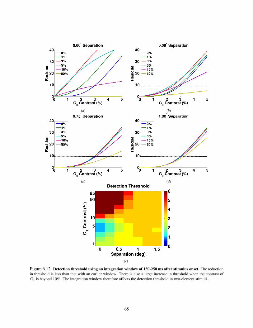
(a) (b)

(c) (d)

(e)

Figure 6.12: Detection threshold using an integration window of 150-250 ms after stimulus onset. The reductionin threshold is less than that with an earlier window. There is also a large increase in threshold when the contrast ofG1 is beyond 10%. The integration window therefore affects the detection threshold in two-element stimuli.

65

(a) (b)

(c) (d)

Figure 6.13: Time course and spatial profiles at different time points for an example configuration of stimuli.(a) Time courses of the center responses to the stimuli containing both overlapping elements (blue), G1 only (green),and the difference between them (residue; red). The contrasts of G0 and G1 are 1.5% and 10%, respectively. Theresponse to the benchmark (3% contrast G0; black) is also plotted. The stimulus was presented from 0 to 220 ms(vertical dashed line) and disappeared after that, and the responses started to drop at about 250 ms. (b)-(d) Spatialprofiles of the responses and the residue at 3 different time points. The relationship between the residues and thebenchmark changes over time, which explains why the thresholds are usually higher when the integration windowstarts late.

i.e. below 3%, up to a G1 contrast of about 12% (Figure 6.14b). The reduction in threshold for the seconddecoder is smaller and only occurs when the contrast ofG1 is below 5%. Beyond that, the threshold increasesvery rapidly (Figure 6.15b).

6.4.4 Proposed psychophysical experiments with VSDI

Because the predicted detection threshold is more sensitive to the integration window for the center-surroundstimuli, they should be used instead of the two-element stimuli in psychophysical experiments to study howthe interactions affect perception and how population responses in V1 should be read out by higher level

66

(a) (b)

Figure 6.14: Detection threshold using an integration window of 50-150 ms after stimulus onset for the center-surround stimulus. (a) The residue as a function of G0 contrast for different background contrasts. (b) Detectionthreshold as a function background contrast. The dashed line plots the benchmark threshold of 3% contrast. There isa reduction in threshold even with medium background contrast.

(a) (b)

Figure 6.15: Detection threshold using an integration window of 150-250 ms after stimulus onset for the center-surround stimulus. (a) The residue as a function of G0 contrast for different background contrasts. (b) The detectionthreshold increases dramatically when the background contrast is higher than 5%, which is different from the predic-tion using an earlier integration window, suggesting that the timing of the window affects the threshold significantlyfor center-surround stimuli.

areas. A simple reaction-time visual detection task with simultaneous VSDI recording that is similar to theexperiment described in Y. Chen et al. (2006, 2008) can be used for such a study. In each trial, after themonkey establishes fixation, the stimulus appears briefly, e.g. 300 ms, at a fixed location. In the center-present trials, the monkey has to shift gaze to the center element of the stimulus within a short time period,e.g. 600 ms, after stimulus onset to get the reward. For center-absent trials, the monkey has to remain fixatedfor an additional time period, e.g. 1 s, after stimulus offset to obtain the reward. In a block of experiment,the surround element is at the fixed contrast, while several, e.g. 5, different contrast levels that span the

67

monkey’s detection threshold are tested for the center element. The numbers of center-present and center-absent trials in each block are the same and the different conditions are interleaved pseudorandomly. TheVSDI responses are recorded while the monkey is performing the task. Using these measured responses, anoptimal Bayesian decoder for the task can be found to show how the responses should be read out to achievebest performance, which could provide insight on how the responses are used in the monkey’s visual systemby comparing the performance between the monkey and the decoder (Y. Chen et al., 2006, 2008).

6.4.5 Summary

Using a simple decoder that integrates the response and compares it with a predefined fixed level, an in-teresting relationship between the detection threshold and the integration time window was found for thetwo-element and center-surround stimuli. An early integration window results in a larger reduction in de-tection threshold, which is desirable in most cases. If the integration starts later, the threshold is reducedless. Based on this prediction, psychological and physiological experiments can be designed to shed lighton how the neural responses in the primary visual cortex are used in the downstream areas. This result alsodemonstrates how new insight about perception can be gained from the PGC model.

6.5 Conclusion

While a single Gabor element on a uniform background is a widely used stimulus for characterizing theresponses in the visual cortex, it is very different from natural scenes that contain more variation in localcontrast. As the first step towards understanding visual processing in a natural setting, the PGC model wasapplied to two classes of stimuli that are more complicated.

The first class of stimuli contained two Gabor elements at various contrasts and separations. Themodel predicted that the interactions are mainly subadditive. At the center of an element, the interactionwas predicted to vary the most when it is at low contrast. These predictions were used to design the set ofstimuli in the VSDI experiments. Without the model’s prediction, it would be difficult to estimate whichfeature combinations will produce the most interesting behavior. The model is therefore a useful tool fordesigning experiments.

The measured spatial VSDI responses turn out to be similar to the responses of the model over alarge range of stimuli. Specifically, the model predicted that the largest effect of interactions usually occurat locations between the two elements, which is consistent with most of the data. This result illustratesthe importance of modeling the whole spatial region instead of just a single point on the cortex. The PGCmodel can therefore account for most of the interactions observed in the VSDI responses for a large rangeof stimulus configurations, suggesting that the PGC model provides a good approximation to the processingin the visual cortex for spatial interactions of the elements.

The second class of stimuli consisted of a small Gabor element on top of a large Gabor background.The model predicted a systematic change in the linearity of the interactions as the contrasts of the twoGabors were varied. A specific physiological experiment was proposed to verify the prediction. This resultdemonstrates one key advantage of computational models: It can sample many different features of thestimulus to discover systematic changes.

The responses of the PGC model for these two classes of stimuli were also used to predict theinteractions’ effects on perception. Detection threshold of an observer for a particular stimulus configurationis predicted to be highly dependent on the timing of a simple decoder. This result demonstrates that the PGC

68

model can also be used to gain insight on how the high-level areas may use the information available in theV1 responses.

This chapter studied the spatial interactions of stationary stimuli and showed that the model’s pre-dictions are consistent with the VSDI responses. In the next chapter, non-stationary stimuli will be used tovalidate the model.

69

Chapter 7

Spatiotemporal Interactions Between VisualStimuli

Even though the PGC model was motivated by the responses to a single Gabor stimulus, it can accountfor the responses to more general stimuli that consist of two stationary elements with various combinationsof contrasts and separation, as was shown in Chapter 6. To test the generality of the model even further,non-stationary visual stimuli with moving contrast envelopes are used in this chapter. The predictions of themodel were again found to be consistent with VSDI responses, suggesting that PGC is a general, accurate,yet simple model for population responses in the visual cortex.

7.1 Motivation

In the previous chapter, the PGC model was shown to account for the spatial interaction between two Gaborelements with a wide range of combinations of contrasts and separation. These two-element stimuli werestationary, however. A more challenging test for the generality of the model is to use non-stationary stimuli,i.e. stimuli that move around, and verify the predictions with the population responses in V1. This chapterreports such a verification using movies that contain a rotating wedge.

In the remaining of the chapter, the stimuli used will first be described, followed by the predictionsof the model and the results of the VSDI experiment using such stimuli.

7.2 Spatiotemporal stimuli

The non-stationary stimuli studied in this chapter consist of a full-contrast wedge that is 5 angular degreeswide and rotates about the fixation point like a clock hand (Figure 7.1). Such stimuli were used in a previousstudy to obtain a precise retinotopic map of V1 with VSDI (Yang et al., 2007). Possible extensions ofthe model to account for the processing of spatiotemporal stimuli that contain motion within a stationarycontrast envelope, e.g. drifting gratings, will be discussed in Section 8.2.1.

In the full counterclockwise stimulus (CCW movie; Figure 7.1), the wedge first appeared at 45 angu-lar degrees off the vertical meridian (225◦). At each 20 ms, the wedge rotated 5 degrees counterclockwise,until it reached 15 degrees on the other side of the visual field (285◦). After that, the wedge returned toits starting position and the whole sequence repeated. A single sweep of the wedge therefore spanned 60

70

angular degrees and took 240 ms to complete. Although it is an artificial stimulus, it represents a commonsituation in which a moving object appears from behind an occluder and then disappears behind anotheroccluder, e.g. a bird flying across a window. Figure 7.1 shows the stimulus at different times within a cycle.

In addition to the full movie, there was a cut movie where the wedge was only presented between240◦ and 270◦ (CCW cut movie; Figure 7.1). The wedge therefore stopped at the vertical meridian anddid not appear in the right visual field. The presentation time of each wedge with respect to stimulus onsetwas the same as in the full movie. In other words, the wedge only appeared during the middle 120 ms ofthe cycle, and the rest of the frames only contained the uniform background (Figure 7.1). The response forthe first wedge in the cut movie (240◦) can therefore be compared with the response at the same locationwhen the full movie is underway to study the spatiotemporal interactions from previous wedges. If theseresponses are not the same, it implies that the perceived motion at the beginning and in the middle of thewedge’s rotation may be different. Similarly, the response dynamics at the vertical meridian for the twomovies can be compared to investigate whether the wedges in one hemifield (after the wedge in the fullmovie passes 270◦) will affect the responses in the other hemifield.

There were also three extra conditions in which only one wedge in the movie was presented. Again,the timing of the wedge presentation was exactly the same as in the full movie; the wedge was presentedfor 20 ms and the rest of the frames were blank in each cycle. Three wedge locations, 240◦, 255◦, and270◦, were used in the VSDI experiments (Figure 7.1). Note that these wedges were presented at differenttimes within the cycle. The responses for these single-wedge stimuli at their respective locations served asa baseline against which the responses for the movies were compared.

A set of clockwise (CW) stimuli that rotated from 285◦ to 225◦ were also used in a VSDI experiment(Figure 7.2). This set only contained the full movie and the cut movie and not the single-wedge stimuli. Theresponse at the location where the cut movie ends can be compared with that for the full movie to study theeffects of interactions from new, continuing wedges.

7.3 Results of the model

In this section, the representations of the stimuli in the input layer of the model will be described. Themodel’s behavior with these stimuli will then be analyzed, followed by simulation results.

7.3.1 Input to the model

The stimuli described above have two interesting properties that simplify their representation in the model.First, because of the nonlinear retinotopic mapping in the macaque, the wedges are mapped to approximatelyparallel bands on V1. Figure 7.3 shows how the borders of the full movie stimulus in the left visual fieldare mapped to V1 in the right (contralateral) hemisphere. The border at 225◦ is mapped to a line that isposterior to V1 and is horizontal in the figure. As the wedge rotates counterclockwise, its mapping on thebrain shifts in the anterior direction; the 270◦ wedge is mapped along the V1/V2 border that represents thevertical meridian.

Although the width of the wedge increases with eccentricity, the thickness of the band is roughlyuniform because of the corresponding decrease in cortical magnification factor. In addition, for the wedgesat different angular locations, the widths of the bands should be similar because the cortical magnificationfactor at a particular eccentricity is approximately constant across different angles. As will be shown in Fig-ure 7.7, these assumptions are valid. As a result, only the posterior-anterior direction needs to be considered

71

Figure 7.1: Counterclockwise spatiotemporal stimuli in the VSDI experiment. Each row in the figure showssnapshots of the stimulus at five example time points. The counterclockwise (CCW) movie always contained a wedgeat some location. All the other stimuli were derived from the CCW movie by replacing some of the frames with a blankbackground. Each wedge was itself a stationary 100%-contrast grating, with decreasing spatial frequency toward themore peripheral location. The white dot in each snapshot is the fixation point.

72

Figure 7.2: Clockwise spatiotemporal stimuli in the VSDI experiment. The clockwise stimuli are simply thecounterclockwise stimuli in Figure 7.1 running backwards. For the full CW movie, the wedge started at 285◦ androtated toward 225◦. In the cut movie, the wedges outside 240◦ to 270◦ were replaced by uniform background, as inthe corresponding counterclockwise stimuli.

(a) (b)

Figure 7.3: Retinotopic mapping of the stimulus. (a) A fan-shape outline that delineates the movie stimulus in theleft visual field. (b) Image of the cortical vasculature taken through the imaging camera in a VSDI experiment. Thefour colored dashed lines show the approximate cortical representation of the corresponding lines in (a). Magenta lineindicates the V1/V2 border. White rectangle is the 4 mm× 7.5 mm region plotted in Figure 7.7. Figures adapted fromYang et al. (2007).

73

and a wedge in the stimulus can be conveniently represented in the model as a pulse of appropriate widthin the one-dimensional input layer, which represents the stimulus in cortical coordinates after retinotopicmapping (Section 5.1.1).

Based on the VSDI responses of such stimuli (which will be presented in Section 7.4.2), the widthof the pulse is 0.7 mm in the input layer. As the wedge rotates counterclockwise, the pulse shifts in 0.7 mmsteps toward location 0, which corresponds to the V1/V2 border. The clockwise stimuli will move in theopposite direction. Rotation of the wedge in the visual space is therefore mapped to translation in the inputlayer.

The second property of such stimuli is that after the wedge crosses the vertical meridian (270◦),the neural response will “move over” to the other hemisphere. In other words, there is a boundary for theresponse at 270◦. In the model, the vertical meridian therefore corresponds to one end of the modeled regionand the wedges in the ipsilateral side are not represented.

7.3.2 Qualitative analysis

To understand the spatiotemporal dynamics of the responses in the model, first consider a fixed unit in themiddle of the first stage. Suppose the pulse in the input layer starts at a certain distance from the unit andmoves toward it. Before the pulse lands on the unit’s location, it will first fall partially in the unit’s receptivefield. The response of this unit therefore starts to rise. Because the pulse may take several 20-ms steps tomove from the periphery to the center of the receptive field, response can build up significantly before thepulse reaches the unit. On the other hand, responses for the single-pulse stimulus presented at the unit’slocation can only start after the pulse appears. The response of the unit therefore rises earlier in the moviethan in the single-pulse stimulus, resulting in a shorter response latency.

The distance between the location of the unit and the first pulse determines how much faster responsewill rise. If the pulse starts at the unit’s location, the response will not be faster than that when it is presentedalone. On the other hand, if the unit is far from the pulse, the response can already be quite large by the timethe pulse reaches the unit. The further the unit from the first pulse, the faster its response. As a result, fromthe position where the pulse starts moving, the relative latency decreases at the locations along the trajectoryof the pulse.

The upper bound of the latency decrease is determined by the size of the receptive field. Since thepulse moves at a constant speed, the receptive field size limits the time for the pulse to travel from theperiphery to its center. Hence, after a certain time into the movie, the relative latency will be constant forthe rest of the locations through which the pulse passes.

After the pulse reaches the center of a unit, it continues its motion and moves away. The receptivefield summation at the unit therefore decreases gradually, which prolongs the response.

The above analysis applies similarly to the second stage of the model. In summary, the modelpredicts that the response for a movie at a particular location will have a shorter latency than that for thestationary wedge. The relative latency between these two conditions is predicted to increase at the locationsalong the wedge’s motion and is limited by the receptive field sizes.

7.3.3 Simulation results

The above analysis was verified with simulation; the results will be described in this section. To characterizethe spatiotemporal responses, the latency difference between the response for the moving wedge and the

74

single-wedge stimuli will be determined for different locations, allowing quantitative comparison with theVSDI responses.

Model simulation

A 7.5 mm long strip of V1 that corresponds to the collapsed white rectangle in Figure 7.3b was simulated.The strip started at the V1/V2 border at location 0 and ran perpendicular to the border in the posteriordirection. The stimulus duration was 960 ms (four cycles). The parameters of the simulation were: σR,1 =0.63 mm, σN,1 = 0.9 mm, C1 = 3.19, C2 = 2.3, k1 = 1089, and k2 = 2. The widths of the receptivefield and normalization pool were smaller than those in the simulation of spatial interaction described inSection 6.2.3 while the rest of the parameters were the same. The smaller widths were due to the narrowerspatial spread of the VSDI responses for this stimulus, which will be discussed in Section 7.4.2.

Spatiotemporal responses

Figure 7.4 shows the first 800 ms of the model’s spatiotemporal responses for the counterclockwise stimulishown in Figure 7.1. The format of the plots is the same as Figure 4.4. Only the top 4.5 mm of the modeledregion is shown in the figure to compare with the VSDI responses shown later in Figures 7.8 and 7.9. Asthe pulse in the CCW movie moves from 225◦ toward 285◦, it elicits responses that shift up with it. After itpasses through 270◦ (0 mm), the pulse is in the other side of the visual field. The resulting responses will bein the other hemisphere of V1, which is not included in the model.

For the CCW cut movie, in each cycle, the first pulse appears at 3.5 to 4.2 mm and there is noresponse at these locations before that time. On the other hand, the responses at these locations for thefull stimulus have already started to rise because of the previous pulses that appear in earlier locations, asanalyzed in Section 7.3.2. This difference can be easily seen from the responses for these two stimuli at 800ms. The responses for both stimuli at locations around 0 are roughly similar because of the limited receptivefield size. Pulses that appear outside of the receptive field do not contribute to the response, therefore to theunits near location 0, the two movies and hence their responses are the same. In addition, note that for theseunits, the normalization pools are truncated beyond location 0, the boundary of the model region. The lowernormalization activity at these locations results in larger peak responses than the other locations.

Each of the bottom three panels in Figure 7.4 shows the spatiotemporal responses to a differentsingle-pulse stimulus. The responses at around 4.2 mm for the stimulus containing a wedge at 240◦ alonebegin to rise at the same time as with the cut movie, and later with the full movie. For the 255◦ and 270◦

stimuli, the the responses at their peak locations are delayed compared to those for the movie stimuli. Therelative latency of the responses therefore decreases more as the pulse travels, as discussed in the previoussection. Note also that the amplitude of the response at the peak location is only about 20% smaller than thepeak amplitude in the movie.

Figure 7.5 shows the spatiotemporal responses for the two clockwise movies. The stimuli and hencethe responses are the same during the initial part of the cycle. The wedge in the cut movie disappears afterreaching 240◦ and the responses drop together at all locations, as in the case for a briefly presented stimulusdiscussed in Chapter 5. In the full movie, the pulse continues to move beyond 240◦. Because of the spatialspread of the responses, the falling edges are prolonged, as in the previous locations. The model thereforepredicts that the relative latencies of the two movies to be the same at most locations.

75

Figure 7.4: Spatiotemporal responses of the model for the counterclockwise stimuli. Each subfigure plots theresponses for the first 4.5 mm of the modeled region. The corresponding visual angles of three key locations areshown to the left of the y-axis. The responses in all the plots are normalized by the same factor. The responses ataround 4.2 mm (240◦) start to rise earlier than those for the cut movie and the 240◦ pulse alone because the pulsespresented earlier fall into the receptive fields at these locations. As time progresses, the responses for the two moviesbecome more and more similar. Both of the responses begin to rise earlier than the single pulses presented at 255◦ and270◦. The latencies of the responses for the movies and the single pulse at the same location are therefore different.

76

Figure 7.5: Spatiotemporal responses of the model for the clockwise stimuli. The responses for the two moviesare initially the same because the stimuli are the same. The cut movie stops at 240◦ and the responses drop togetherat all locations. In the full movie, the pulse continues to move beyond 240◦, thus extending the falling edges at thoselocations. The responses are therefore different at these locations.

Relative latencies

To compare the time courses of the responses for the movies quantitatively to those for the single-pulsestimuli, the fast Fourier transform was applied to the response at each location for each stimulus to obtainthe phase of the response at the stimulus frequency (4.17 Hz). Then, for each location, the phase of theresponse for the single-pulse stimulus that appears at that location was subtracted from that of the moviestimuli. Finally, this difference in phase angles was converted into time from the length of the stimulus cycleto produce the relative latency. A relative latency of 0 ms at a particular location means that the responsesfor the movie and the corresponding single-pulse stimulus are in phase. A negative relative latency meansthat the response rises earlier for the movie than for the single pulse. The main reason of employing such ameasure of response latency instead of the one used in Section 4.3.2 (i.e. time to rise above 10% of the peakresponse of the sigmoidal fit) is to compare the model’s predictions with the VSDI responses. Unlike theexperiment in Chapter 4, the number of trials for these stimuli was small (∼10) and the Fourier componentsof the VSDI responses provided a much larger signal-to-noise ratio than the raw time courses.

Figure 7.6a shows the relative latencies at different locations for the counterclockwise movies. At4.2 mm (240◦), the latency is already decreased by about 12 ms for the full movie because of the earlierpulses. The relative latency is about 0 ms for the cut movie because this is the location where the firstwedge appears in the stimulus. As the pulse moves closer to location 0 (270◦), the relative latencies of bothstimuli decrease because there are more pulses in earlier locations to increase the response sooner. Finally,the relative latencies for the two stimuli converge because receptive fields have limited size as discussed inSection 7.3.2.

Figure 7.6b shows the relative latencies for the clockwise movies. At the beginning (270◦), therelative latencies for both stimuli are 0 ms because no pulse has yet been presented in the cycle. As in thecounterclockwise stimuli, the relative latency decreases at locations along the motion of the pulse. The tworelative latencies are the same up to about 2 mm (255◦) because the first parts of the movies are the same

77

(a) (b)

Figure 7.6: Relative latencies of the responses. (a) Relative latencies for the counterclockwise stimuli. As shown inFigure 7.4, the latencies for the full movie and the cut movie are different initially at around 4.2 mm. For the cut movie,the relative latency is zero because it is the first location that the pulse appears. The relative latencies for both stimulifall as the pulse moves toward 0 mm and they finally converge as the corresponding responses become the same. (b)Relative latencies for the clockwise stimuli. Initially, the relative latencies for the full movie and the cut movie are thesame. They start to diverge as the relative latency for the full movie stabilizes, whereas for the cut movie, it decreasesas there are fewer pulses moving away to delay the relative latency.

in the modeled hemisphere (Figure 7.2). The relative latency for the full stimulus stabilizes during the laterpart of the movie because of the limited receptive field size; a steady relationship between the responses tothe full movie and the single pulse stimuli has been reached. For the cut movie, there is a further drop inrelative latency at locations near the end because the responses at these locations are shorter than those forthe full movie (Figure 7.5). The peaks of the response hence occur earlier, resulting in larger decrease inlatency because the phase of the Fourier component is closely related to the time-to-peak of the response.

In summary, the model predicts that after the movie has started, the latency of the response is de-creased relative to that for a single wedge presented at the same location. Such decrease is due to theprevious wedges in the movie because the responses to the first wedge are not accelerated (Figure 7.6a). Onthe other hand, the wedges that appear later in the movie counteract with such decrease. When the moviestops, such counteraction disappears, resulting in a larger latency decrease (Figure 7.6b). These predictionswill be compared with the VSDI responses next.

7.4 VSDI experiment

In this section, the details of the VSDI experiment will be described, followed by the same analyses of thepopulation responses that were applied to the model’s responses.

7.4.1 Experimental procedures and data analysis

The stimuli shown in Figures 7.1 and 7.2 were presented to a fixating monkey as a part of an experiment toobtain a precise retinotopic map of V1 with VSDI (Yang et al., 2007). This animal is different from those

78

in the experiments described in the previous chapters. In each trial, seven cycles of the same stimulus werepresented, for a total of 1680 ms. The length of the wedge spanned from 1.32◦ to 4.2◦ visual angle, i.e.2.88◦ long. In the experiment reported in this section, there were 11 trials for each condition.

The VSDI signals were processed by the procedures that were similar to those described in Sec-tion 4.2.2. The region of interest (ROI) where the VSDI signals were analyzed is shown in Figure 7.3b. Aswas discussed in Section 7.3.1, the response to a wedge in V1 is a band of roughly uniform width along thelateral-medial direction, which is horizontal in this region. The VSDI signals were subsequently averagedacross the width of the region to obtain a one-dimensional response.

The top of the ROI was located roughly at the V1/V2 border (vertical meridian), which can beestimated from the VSDI responses of the movie stimulus. Due to the symmetric but opposite mappings ofpolar angles in V1 and V2, as the wedge rotates toward the vertical meridian, the responses in these twoareas move toward each other. When the wedge is at 270◦, i.e. vertical, these two responses converge. Theline of convergence thus corresponds to the V1/V2 border.

To derive the relative latencies of different stimuli, for each location and for each trial, the Fourierphases of the time courses at the stimulus frequency (4.17 Hz) were extracted after removing the averagesignal of the blank condition.

7.4.2 Results

In this section, the peak spatial responses for stimuli consisting of a single wedge will be presented first toshow the mapping of the wedges on V1. After that, the spatiotemporal responses and their relative laten-cies will be presented. The properties of the VSDI responses are consistent with the model’s predictions,suggesting that population gain control is a general mechanism for visual processing.

Peak spatial responses for single wedges

Figure 7.7 plots the normalized peak spatial responses in the region of interest (white rectangle in Figure 7.3)for the stimuli that contained only a single wedge at the labeled location. As can be seen in the plots, theresponses form horizontal bands of roughly uniform width. The average width (σ) of the Gaussian fits for thespatial responses for all vertical slices is 1.05 mm, which is narrower than those observed in the experimentsdiscussed in previous chapters (2.1 mm). Such difference may be due to the variations in individual animalsand is unlikely to be due to the widths of the stimuli because they are all very small.

Each time the wedge was rotated by 30◦, the corresponding responses shifted by about 2.1 mm. Themapping of polar angle to the cortex is hence approximately linear. A distance of 5 angular degrees thereforemaps to 0.7 mm, which was used as the width of the pulse in the input layer of the model.

Because the VSDI responses are similar in the horizontal direction, they were averaged and collapsedinto one-dimension responses that ran vertically from the V1/V2 border in the posterior direction, which isthe region that the input layer of the model represents.

Spatiotemporal responses

The average spatiotemporal responses of the collapsed region for different counterclockwise stimuli areplotted in Figure 7.8. Only the responses in the top 4.2 mm of the ROI were plotted because the responsesin the bottom part are noisy. The first 800 ms after stimulus onset are shown, and all the responses werenormalized by the same scale. As predicted by the model, the responses at around 4.2 mm from the V1/V2

79

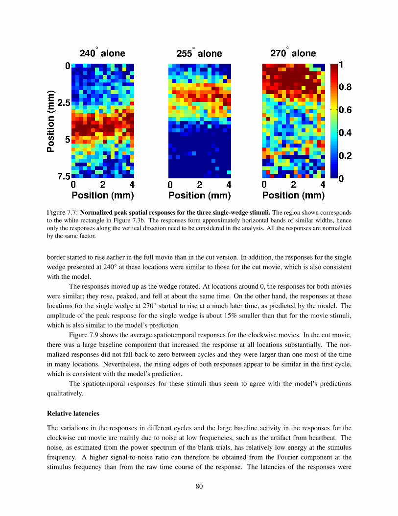
Figure 7.7: Normalized peak spatial responses for the three single-wedge stimuli. The region shown correspondsto the white rectangle in Figure 7.3b. The responses form approximately horizontal bands of similar widths, henceonly the responses along the vertical direction need to be considered in the analysis. All the responses are normalizedby the same factor.

border started to rise earlier in the full movie than in the cut version. In addition, the responses for the singlewedge presented at 240◦ at these locations were similar to those for the cut movie, which is also consistentwith the model.

The responses moved up as the wedge rotated. At locations around 0, the responses for both movieswere similar; they rose, peaked, and fell at about the same time. On the other hand, the responses at theselocations for the single wedge at 270◦ started to rise at a much later time, as predicted by the model. Theamplitude of the peak response for the single wedge is about 15% smaller than that for the movie stimuli,which is also similar to the model’s prediction.

Figure 7.9 shows the average spatiotemporal responses for the clockwise movies. In the cut movie,there was a large baseline component that increased the response at all locations substantially. The nor-malized responses did not fall back to zero between cycles and they were larger than one most of the timein many locations. Nevertheless, the rising edges of both responses appear to be similar in the first cycle,which is consistent with the model’s prediction.

The spatiotemporal responses for these stimuli thus seem to agree with the model’s predictionsqualitatively.

Relative latencies

The variations in the responses in different cycles and the large baseline activity in the responses for theclockwise cut movie are mainly due to noise at low frequencies, such as the artifact from heartbeat. Thenoise, as estimated from the power spectrum of the blank trials, has relatively low energy at the stimulusfrequency. A higher signal-to-noise ratio can therefore be obtained from the Fourier component at thestimulus frequency than from the raw time course of the response. The latencies of the responses were

80

Figure 7.8: Spatiotemporal VSDI responses for the counterclockwise stimuli. The responses are normalized bythe same scale as in Figure 7.7. The responses for the full movie start to rise earlier than those of the cut movie andthe 240◦ wedge at around 4.2 mm. At around 0 mm, the responses for the two movies are similar and rise earlier thanthe 270◦ wedge. The model’s predictions (Figure 7.4) are therefore consistent with the VSDI responses.

81

Figure 7.9: Spatiotemporal VSDI responses for the clockwise stimuli. There is a large baseline noise for the cutmovie between 200 to 700 ms, saturating the color scale. The noise has mostly low frequency, and a higher signal-to-noise ratio can be obtained by considering the Fourier amplitude at the stimulus frequency to compute the relativelatencies as in Figure 7.10.

hence estimated using the phase of that Fourier component.The relative latencies for different movie stimuli of the VSDI responses were computed using the

same method used for the model’s responses. There were only three single-wedge locations tested in theexperiments. The latencies of these responses were interpolated to estimate the latencies at the locations inbetween them. In addition, since the timing for the single-wedge stimuli matched only the counterclockwisemovies, the latencies of these stimuli for the clockwise timing were estimated from those at the mirrorlocations of their counterclockwise counterparts.

Figures 7.10a and b plot the relative latencies at different locations for the counterclockwise andclockwise movies, respectively. The error bars are the 95% bootstrap confidence intervals and the solid linesare the predictions of the model in Figure 7.6. These lines lie within the confidence intervals for all stimuliat all locations, suggesting that the model provides an accurate description of the spatiotemporal dynamicsof VSDI responses for the movie stimuli.

To investigate whether the decrease in latency can be explained solely by linear receptive fields,a model that uses the average VSDI responses to a single 255◦ wedge as the “spatiotemporal impulse re-sponse” to a single wedge was simulated. For each wedge in the movie, the impulse response was added tothe model at the corresponding time and space to produce the response. The relative latencies of this modelare plotted in dashed lines in Figure 7.10, which have a similar behavior to the data, suggesting that thedecrease in response latency in the movies could be accounted for to a large extent by linear receptive fields.However, the responses in the linear model for a movie can be three times larger than that for a single wedgebecause of the spatial spread of the responses. The difference observed between the amplitudes of these tworesponses is only 15%, which is inconsistent with the linear model. On the other hand, because of gain con-trol, the responses for the movies in the PGC model are only 20% larger than those for a single wedge. Thisresult demonstrates the important role of normalization: It keeps the response within the dynamic range.

Normalization also contributes to the decrease in latency in the second stage of the model. Because

82

(a) (b)

Figure 7.10: Relative latencies of the VSDI responses and the model’s predictions. Error bars are 95% bootstrapconfidence interval. The solid lines are the predictions of the model from Figure 7.6. The dashed lines are linearpredictions based on the VSDI responses to a single wedge. The model’s predictions are consistent with the data,suggesting it is a general model of visual processing.

the response time courses are continuous in the first stage, the spatial normalization pool of the second stagewill include the first-stage responses elicited by previous pulses. At a particular location, the normalizationactivity will build up over time as the pulse moves toward it. As a result, the time constant of the rising edgeof the response will be smaller than that for the single pulse, leading to a shorter latency. In the first stage,the normalization pool does not include activity from previous pulses because the input activity simply turnson and off instantly as the pulse moves along the input layer.

7.5 Discussion

The PGC model can account for the spatiotemporal dynamics of V1 population responses simultaneouslyfor different stimuli

7.5.1 Model parameters

The shorter response latency in moving stimuli reported in this chapter has also been observed in the retinalganglion cells of the salamander and rabbit using similar stimuli (Berry, Brivanlou, Jordan, & Meister,1999). This result suggests that some of the latency decrease observed in V1 may come from subcorticalareas. Coincidentally, a single-site contrast gain control model similar to PGC was used to account for suchlatency decrease in the retina (Berry et al., 1999), echoing the idea that gain control occurs in multiple stagesin the visual pathway, as discussed in Chapter 5. To model the responses in V1, it is therefore inaccurate toassume that subcortical areas are linear, as they are in many models.

Interestingly, the decrease in response latency for a moving stimulus is consistent with a visualillusion called the flash-lag effect in which a flash and a moving object that appear in the same location areperceived to be displaced from one another (Mackay, 1958; Nijhawan, 1994; Whitney & Murakami, 1998;

83

Eagleman & Sejnowski, 2000). If response latency alone is used to determine the timing and position of thestimulus, the flash-lag effect will be smaller if the moving object travels for a shorter distance before the flashobject is presented because the relative latency is smaller. On the other hand, the same argument implies thatthe initial motion of the moving wedge will be perceived as slower because the limit of decrease in latencyhas not yet been reached. This implication seems unlikely and more experimental and computational studiesare required to understand how motion and position are perceived.

7.6 Conclusion

In this chapter, the PGC model was applied to moving stimuli. Such stimuli constitute a challenging testfor the generality of the model, which was based on the observations in the responses of small stationarystimuli.

The model predicted that the responses in a movie would have a shorter latency than a stationarywedge at the same location. The relative latency between these two conditions was predicted to increasein locations along the wedge’s motion and was limited by the receptive field sizes. These predictions werefound to be consistent with the VSDI responses of such stimuli. Specifically, the values of the relativelatencies at different locations for the full movies and their cut versions agreed with the model’s predictions.The relative latencies for different parts of the movie can therefore be explained by the PGC model.

The PGC model is the first model that can account for the spatiotemporal dynamics of V1 popu-lation responses simultaneously for different stimuli containing (1) a single Gabor element, (2) two Gaborelements, and (3) a wedge that rotates at constant speed, suggesting that it is a general, accurate, yet simplemodel for visual processing.

84

Chapter 8

Discussion and Future Research

The results in the previous chapters show that the PGC model in which a unit represents a local populationof neurons with different stimulus preferences can account for the spatiotemporal responses in V1 for dif-ferent types of stimuli. For each of the stimuli, different receptive field and normalization pool sizes wereused in the model simulation. Moreover, the current model does not take into account fine-scale corticalstructure, such as orientation columns. This chapter discusses the issue of using different model parametersfor different stimuli first, and then outlines how fine-scale structures can be modeled in future work andproposes further research directions with such an extension. More specifically, the extended model can beused to (1) (1) analyze the network’s stability, (2) study the neural code for orientation, (3) investigate howthe model can be extended to development, and (4) how it can be used to simulate high-level areas.

8.1 Model parameters

In the simulations of the model, the receptive field and normalization pool sizes were different for the threeclasses of stimuli used in Chapters 5, 6, and 7, due to the different spatial spreads observed in the VSDIresponses. It is possible that such difference in sizes is mainly due to individual variations between theanimals, as a different animal was used in each experiment. Another possibility is that for different stimuli,slower processes such as adaptation and homeostasis may take place and change the operating point ofthe neural population. However, given the relatively short stimulus presentation (∼1 s) and long intertrialinterval (6-8 s) for all the stimuli, these processes should result in similar operating points. In addition, themonkeys were only required to maintain fixation in all the experiments, hence any high level task-relatedmodulations in V1 should be similar and should not affect the sizes of the receptive fields and normalizationpools.

A straightforward way to test these arguments is to use a single animal with the three classes ofstimuli. If the spatial spreads of the VSDI responses are the same and a single set of model parameterscan be used to account for the responses, it will support the argument that the difference reported in thisdissertation is due to individual variations. Otherwise, more investigations will be required to study how theoperating points of the neural population change with stimuli and how the model can be extended to accountfor it.

Finally, the change in parameters may due to other mechanisms that the model omits, which causerelatively small errors for the specific experimental data shown in this dissertation. As in any model, theseomitted mechanisms may turn out to be important and prevent the model from being valid in general over

85

a wide range of conditions. Further experiments using different types of stimuli are required to address thisimportant question.

8.2 Extension to fine spatial scales

A unit in the PGC model represents a local population of neurons that spans several orientation columns.Extending the PGC model to the orientation-column level is therefore a logical and important next step.Such an extension will require that the connectivity in V1 is represented in detail: There are extensivelateral and feedback connections in V1 that link neurons with similar orientation preference and presumablyplay a role in information processing (Fisken et al., 1975; Gilbert & Wiesel, 1979, 1983; Hirsch & Gilbert,1991; Bosking et al., 1997; Angelucci, Levitt, Walton, et al., 2002). However, little is known about howexactly they do it. Extending the PGC model to include such connections should provide insight into thisopen question.

In the experiments in this dissertation, orientation-related signals are weak in the VSDI responsebecause a relatively low spatial resolution was used to image the active region of V1. At a higher resolution(which is possible with current technology) the responses from individual columns will be stronger and thepredictions of the extended model can be tested experimentally.

In this section, a possible representation of orientation-specific signals will be discussed, followedby an outline of different formulations that can incorporate such signals into the model. Extensions forother properties at fine spatial scales such as direction selectivity should follow similar formulations. Theremaining sections of this chapter outline future research directions that the extended model makes possible.

8.2.1 Modeling orientation-specific signals in lateral and feedback connections

Orientation-specific signals occur only in the second stage of the model because the subcortical areas, whichthe first stage of the model represents, are not orientation-selective. All the variables in this chapter thereforerefer to the second stage of the model and the first stage will remain the same.

In the extended model, a unit is labeled not only by its receptive field location x, as in the originalPGC model, but also by its orientation preference θ. In addition, the receptive field of a unit is a Gaborfunction with orientation θ, instead of its Gaussian envelope. The receptive field can also be extended tomodel other response properties such as direction selectivity that the current PGC model does not take intoaccount. The formulation of the model for these properties will be similar to the extensions discussed in thissection.

Since the unit responses represent membrane potentials, they have to be transformed into spikingactivity through a power function before sending them out to other units (Section 5.1.4). Connectionsbetween units are assumed to have the same pattern for all units represented by a spatiotemporal kernelGo(x, θ, t). The spatial component of the kernel represents the connection weights from the units at differentrelative locations and orientation preferences, and the temporal component models the conduction speed ofthese connections. Thus, the orientation-specific signal R(x, θ, t) received by the unit (x, θ) at time t is

R(x, θ, t) = V (x, θ, t)n ⊗Go(x, θ, t), (8.1)

where ⊗ denotes convolution.

86

8.2.2 Possible extensions of the PGC model for orientation-specific signals

One way to incorporate orientation-specific signals into the model is to treat them as external inputs, as inmany previous models using LN units (Miikkulainen et al., 2005; Sirosh & Miikkulainen, 1994), and leakyintegrators (Wilson & Cowan, 1973; Amari, 1977; Ben-Yishai et al., 1995; Somers et al., 1995; Hansel &Sompolinsky, 1998) that were reviewed in Chapter 3. More specifically, these signals are represented as anextra input current into the RC circuit of the model while the other variables remain the same. The extendedmodel then becomes

C∂V (x, θ, t)

∂t= R(x, θ, t) +A(x, θ, t)− g(x, t)V (x, θ, t). (8.2)

Note that the conductance g(x, t) does not depend on orientation because the normalization activity is as-sumed to be unselective for orientation in this extension, as in the original PGC model. Conductance that isa function of the orientation-specific signals will be discussed later in this section.

The dynamics of the responses impose constraints on the properties of the orientation-specific sig-nals. For example, after the stimulus presentation, the driving currentA(x, θ, t) will be zero everywhere andequation 8.2 becomes

C∂V (x, θ, t)

∂t= R(x, θ, t)− g0V (x, θ, t). (8.3)

For the response to decay, the following inequality has to be satisfied:

R(x, θ, t) < g0V (x, θ, t) (8.4)

V (x, θ, t)n ⊗Go(x, θ, t) < g0V (x, θ, t). (8.5)

One way to satisfy this inequality is to make all the components in Go(x, θ, t) negative, assuming thecondition V (x, θ, t) ≥ 0 is maintained in the model e.g. by rectification. In other words, the interaction isinhibitory.

Instead of changing the inputs directly, another possible role of the orientation-specific interactionsis to adjust the conductance and hence the gain of the neurons. Such interactions can be additive, i.e.

g(x, θ, t) = g0(1 +B(x, t) +R(x, θ, t)), (8.6)

or multiplicative, i.e.g(x, θ, t) = g0(1 +B(x, t))(1 +R(x, θ, t)). (8.7)

In the formulation 8.6 and 8.7, the orientation-specific signals increase conductance, which leads to fastertemporal dynamics and a suppressed response.

It is also possible for these signals to affect both the input and the gain of the units. However, as anext step, it is useful to study them individually so that the resulting response properties can be characterizedseparately.

These extensions can be approximated by the original PGC model in certain cases where the orientation-specific signal is small. Anatomically, the lateral connections to nearby neurons are relatively unspecific,but at longer distances they tend to connect neurons with similar orientation preferences (Amir, Harel, &Malach, 1993; Malach, Amir, Harel, & Grinvald, 1993; Bosking et al., 1997; Sincich & Blasdel, 2001).For stimuli that consist of single small elements (such as those used in Chapter 4), these signals are similararound the center of the stimulus and are thus not orientation-specific. As a result, the conductance depends

87

only on x and t at these locations and can be written as g′0(1+B′(x, t)), which is of the same form as in thePGC model.

For stimuli consisting of two elements (such as those used in Chapter 6), the orientation-specificsignals from one element will suppress the responses for the other element. Because of the conductionspeed of the lateral and feedback connections, such an effect will have a delay that depends on distance.As a result, if the stimulus is presented periodically, for a certain range of separation, the suppression fromone element can coincide with the falling edge of the responses to the other element, thus resulting instronger modulation. The extended model could therefore explain the larger modulation observed in theVSDI responses at some separations (Section 6.2.4).

8.3 Analysis of the extended model

The delayed suppression in the extended model can cause oscillations in the responses when the kernelGo(x, θ, t) satisfies certain conditions, e.g. the suppression is too strong. While coherent oscillations havebeen observed in the spiking activity of a small group of neurons (see e.g. Jefferys, Traub, and Whittington(1996) and Buzsaki and Draguhn (2004) for review), VSDI responses do not seem to oscillate. One funda-mental question for the extended model is therefore under what conditions the fixed points of the networkare stable?

In fact, equation 8.2 is a generalization of the Hopfield network (Hopfield, 1982), whose stabilityhas been analyzed thoroughly (Marcus & Westervelt, 1989; Belair, Campbell, & van den Driessche, 1996;Wang, Liu, & Liu, 2005; Liao, Liu, & Zhang, 2006; B. Chen & Wang, 2007; Shao, 2008). However, theconductance in a Hopfield network is constant, whereas in the extended model it depends on the pooledactivity. It is therefore an open question how the stability analyses of Hopfield networks apply to a modeldescribed by equation 8.2. The conditions for stable fixed points will provide new insight on the generalpatterns of orientation-specific connections.

In addition, based on the stability conditions derived from the different formulations of interactions,new experiments can be designed to differentiate them, which should lead to a better understanding of therole of lateral connections in visual processing.

8.4 Decoding orientation-specific neural response

Chapter 6 demonstrated how the PGC model can be used to gain insight on how high-level areas may usethe information available in the V1 responses to detect stimuli. A similar approach can be used with theextended model for orientation-related tasks.

The orientation tuning of most V1 neurons in the monkey is quite wide (∼ 25◦ half-bandwidth;Schiller et al., 1976; De Valois et al., 1982; Ringach et al., 2002), however, a monkey can discriminate twogratings that differ by only 2◦ in orientation after training (Vogels & Orban, 1990). How can such a lowthreshold be achieved with responses that are so broadly tuned? Is there a best time window to integrate theresponse? These questions can be addressed by analyzing the responses of the extended model.

Another related future direction is to use the model’s responses to design better decoders. Thetemporal integration method used in Chapter 6 is very simple. For a specific task, decoders that have ahigher accuracy can be constructed by taking the spatiotemporal properties of the population responses andnoise into account (Y. Chen et al., 2006, 2008). It is likely that the responses in V1 are used in different ways

88

for different tasks. Using a model that can represent the response dynamics accurately, efficient decoders canbe built for a new task or stimulus without acquiring the actual neural responses for all possible conditions.One interesting potential application of such decoders is neural prosthetics, where the responses from themodel can be used to train the controllers to read out the neural signals.

8.5 Network implementation of the model

Two-dimensional self-organizing networks have been successful in explaining how the orderly structure ofthe feature maps in V1 can develop in a network that is initially unorganized (von der Malsburg, 1973;Kohonen, 1982, 2001; Sirosh & Miikkulainen, 1994; Bednar, 2002; Miikkulainen et al., 2005). However,the units in these models do not take into account the temporal properties of the responses. By replacingthese units with an implementation of the extended model, a self-organizing network with accurate responsedynamics and lateral interaction can be built.

Such an extension is important because visual stimuli entering the eyes are constantly changingdue to the motion in the environment and the observer’s own movement. A model that can represent thespatiotemporal dynamics of the response accurately is therefore needed to study how selectivity and orga-nization can develop in such conditions. In particular, many V1 neurons are selective to the direction ofmovement of the stimulus and an accurate description of response dynamics will be important to accountfor how such a selectivity arises.

8.6 Modeling higher level areas

Given the limited dynamic range of spiking activity, population gain control is a simple and effective mech-anism that can maintain the sensitivity and tuning of neurons over a large range of sensory stimuli. It istherefore possible that population gain control operates in most, if not all, sensory cortical areas. Interest-ingly, a normalization model that is similar to the PGC model was used recently to reconcile alternativetheories of attention (Reynolds & Heeger, 2009), suggesting that normalization occurs in high-level areas aswell.

The visual pathway could therefore be simulated by a cascade of PGC models, each representing afunctional area. Such a computational model would be important to understand the processing that takesplace in each visual area after V1. In fact, little is known even for the immediate downstream area of V1,the secondary visual cortex (V2; Boynton & Hegde, 2004). Realistic computational models can be usedto provide verifiable predictions on the receptive field properties and the computation that is carried out inthese areas, and eventually allow us to understand the role of these areas in visual processing.

8.7 Conclusion

This chapter outlined future extensions based on the work in this dissertation, focusing on providing insightinto visual processing at a more fine-grained level than in the current PGC model. In particular, theoret-ical constraints on the orientation-specific connections and their effects on the response dynamics can bederived from the extension. Such an extension can also provide insight into how high-level areas may useorientation-specific information in V1. In addition, detailed network models that have realistic responsedynamics and interaction can be built to study how the orderly organization in V1 can develop through

89

input-driven self-organization. Such models can also provide verifiable predictions on the processing inhigher-level areas, thus advancing our understanding of the visual system more broadly.

90

Chapter 9

Conclusion

The results in this dissertation show that even a simple stimulus can elicit a response that exhibits system-atic and unexpected nonlinear properties. Most existing models are inconsistent with these properties. Thisdissertation proposes the population gain control (PGC) model, which is a generalization of normalizationmodels. The PGC model can account for the spatiotemporal dynamics of the responses for a variety ofstimuli, suggesting that population gain control is a general mechanism of cortical processing. It is thereforepossible that population gain control operates in most, if not all, sensory cortical areas. If so, then the popu-lation dynamics reported in V1 may be observed in many other cortical areas as well, and the correspondingpathways may be understood computationally as a cascade of PGC models.

9.1 Contributions

In Chapter 4, the first quantitative description of the spatiotemporal dynamics of V1 population responses toa briefly presented localized visual stimulus was provided. The population responses exhibited systematicand unexpected nonlinear properties that are not obvious from single-unit recordings. These results demon-strate that unexpected properties can emerge at the level of neural populations, and that it is important tocharacterize population responses quantitatively in both space and time. More importantly, these propertiesare not consistent with most existing models of neural computation, suggesting a new model is required toaccount for them.

Chapter 5 showed that a simple canonical PGC model can account for the spatiotemporal dynamicsof the response to a small stimulus. The PGC model was also used to address the outstanding questionregarding the degree to which nonlinearities in V1 responses are inherited from its inputs. The PGC modelpredicts how the responses to a large stimulus depend on the nonlinearity in V1 and its input. Results froman additional VSDI experiment that varied stimulus size were consistent with the hypothesis that most ofthe response nonlinearity observed in V1 is inherited from its input. This result suggests that most of thegain control for a small localized stimulus may be implemented before the superficial layers of V1. It alsoillustrates how a computational model can be used not only to replicate the behavior of the responses, but togain new insight about visual processing as well.

Chapter 6 discussed the predictions of the PGC model for V1 population responses to more compli-cated spatial stimuli that contain two elements. The model was used to pinpoint a small set of stimuli thatwas expected to be most informative for characterizing the interactions between the two elements. Thesestimuli were then used subsequently in VSDI experiments. The properties of the observed VSDI responses

91

were largely consistent with the model’s predictions, suggesting that population gain control is a generalmechanism for visual processing.

A second class of stimuli, consisting of a small Gabor element on top of a large Gabor background,was also studied in Chapter 6. The model predicted that linearity of the interaction would change systemati-cally as the contrasts of the two Gabors vary. A specific physiological experiment was proposed to verify thisprediction. This result demonstrates one key advantage of computational models: It is possible to samplemany different features of the stimulus to discover systematic changes.

The model’s responses for these two classes of stimuli were then used to predict how the interactioncan affect perception, providing insight on how neural responses may be decoded in the brain.

In Chapter 7, the PGC model was applied to moving stimuli. Such stimuli constitute a challengingtests for the generality of the model, which was based on the observations in the responses of small sta-tionary stimuli only. The model predicted that the responses in a movie would have a shorter latency thana stationary wedge at the same location. The relative latency between these two conditions was predictedto increase in locations along the wedge’s motion and to be limited by the receptive field sizes. These pre-dictions were consistent with the VSDI responses of such stimuli. Specifically, the values of the relativelatencies at different locations for the full movies and their cut versions agreed with the model’s predictions,suggesting that it is a general, accurate, yet simple model for population responses in the visual cortex.

9.2 Conclusion

PGC is a new model for large neural populations that takes into account the dynamics of the responses. Itprovides a promising foundation for further research on neural computation at the population level in othercortical areas. Different interconnected areas can also potentially be simulated by cascading the PGC modelsto study their interactions. Eventually, a complete functional pathway may be simulated accurately usingPGC models, thus advancing our understanding of large-scale neural computation in a way that cannot beachieved by low-level biophysical models.

This dissertation shows that the complete spatiotemporal dynamics of large neural populations canbe specified by a single PGC equation. The premise of this equation is the simple idea of gain controlby response pooling, which can be implemented through the vast network in the brain. The results in thisdissertation therefore suggest that not only is there a general principle for neural processing in the complexnetwork of the brain, but it is a simple one as well.

92

Bibliography

Abbott, L. F., & van Vreeswijk, C. (1993). Asynchronous states in networks of pulse-coupled oscillators.Physical Review E, 48(2), 1483–1490.

Abbott, L. F., Varela, J. A., Sen, K., & Nelson, S. B. (1997). Synaptic depression and cortical gain control.Science, 275(5297), 220–224.

Albrecht, D. G. (1995). Visual cortex neurons in monkey and cat: effect of contrast on the spatial andtemporal phase transfer functions. Visual Neuroscience, 12(6), 1191–1210.

Albrecht, D. G., & Geisler, W. S. (1991). Motion selectivity and the contrast-response function of simplecells in the visual cortex. Visual Neuroscience, 7, 531–546.

Albrecht, D. G., Geisler, W. S., Frazor, R. A., & Crane, A. M. (2002). Visual cortex neurons of monkeysand cats: Temporal dynamics of the contrast response function. Journal of Neurophysiology, 88(2),888–913.

Albrecht, D. G., & Hamilton, D. B. (1982). Striate cortex of monkey and cat: contrast response function.Journal of Neurophysiology, 48(1), 217–237.

Amari, S. (1977). Dynamics of pattern formation in lateral-inhibition type neural fields. Biological Cyber-netics, 27(2), 77–87.

Amir, Y., Harel, M., & Malach, R. (1993). Cortical hierarchy reflected in the organization of intrinsicconnections in macaque monkey visual cortex. Journal of Comparative Neurology, 334, 19–46.

Anderson, J. S., Lampl, I., Gillespie, D. C., & Ferster, D. (2000). The contribution of noise to contrastinvariance of orientation tuning in cat visual cortex. Science, 290(5498), 1968–1972.

Angelucci, A., Levitt, J. B., & Lund, J. S. (2002). Anatomical origins of the classical receptive field andmodulatory surround field of single neurons in macaque visual cortical area V1. Progress in BrainResearch, 136, 373–388.

Angelucci, A., Levitt, J. B., Walton, E. J., Hupe, J. M., Bullier, J., & Lund, J. S. (2002). Circuits for localand global signal integration in primary visual cortex. Journal of Neuroscience, 22, 8633–8646.

Angelucci, A., & Sainsbury, K. (2006). Contribution of feedforward thalamic afferents and corticogeniculatefeedback to the spatial summation area of macaque V1 and LGN. Journal of Comparative Neurology,498(3), 330–351.

Bair, W., Cavanaugh, J. R., Smith, M. A., & Movshon, J. A. (2002). The timing of response onset and offsetin macaque visual neurons. Journal of Neuroscience, 22(8), 3189–3205.

Bednar, J. A. (2002). Learning to see: Genetic and environmental influences on visual development.Unpublished doctoral dissertation, Department of Computer Sciences, The University of Texas atAustin, Austin, TX. (Technical Report AI-TR-02-294)

Belair, J., Campbell, S. A., & van den Driessche, P. (1996). Frustration, stability, and delay-inducedoscillations in a neural network model. SIAM Journal on Applied Mathematics, 56(1), 347–255.

93

Ben-Yishai, R., Bar-Or, R. L., & Sompolinsky, H. (1995). Theory of orientation tuning in visual cortex.Proceedings of the National Academy of Sciences, USA, 92, 3844–3848.

Berry, M. J., Brivanlou, I. H., Jordan, T. A., & Meister, M. (1999). Anticipation of moving stimuli by theretina. Nature, 398, 334–338.

Blasdel, G. G., & Campbell, D. (2001). Functional retinotopy of monkey visual cortex. Journal of Neuro-science, 21(20), 8286–8301.

Bonin, V., Mante, V., & Carandini, M. (2005). The suppressive field of neurons in lateral geniculate nucleus.Journal of Neuroscience, 25, 10844–10856.

Bosking, W. H., Zhang, Y., Schofield, B. R., & Fitzpatrick, D. (1997). Orientation selectivity and thearrangement of horizontal connections in tree shrew striate cortex. Journal of Neuroscience, 17(6),2112–2127.

Boynton, G. M., & Hegde, J. (2004). Visual cortex: The continuing puzzle of area V2. Current Biology,14(13), R523–R524.

Burkitt, A. N. (2006a). A review of the integrate-and-fire neuron model: I. Homogeneous synaptic input.Biological Cybernetics, 95(1), 1–19.

Burkitt, A. N. (2006b). A review of the integrate-and-fire neuron model: II. Inhomogeneous synaptic inputand network properties. Biological Cybernetics, 95(2), 97–112.

Buzsaki, G., & Draguhn, A. (2004). Neuronal oscillations in cortical networks. Science, 304, 1926–1929.Cannon, M. W., & Fullenkamp, S. C. (1993). Spatial interactions in apparent contrast: Individual differences

in enhancement and suppression effects. Vision Research, 33(12), 1685–1695.Carandini, M. (2004). Receptive fields and suppressive fields in the early visual system. In M. Gazzaniga

(Ed.), The cognitive neurosciences III (pp. 313–326). MIT Press.Carandini, M., & Heeger, D. J. (1994). Summation and division by neurons in primate visual cortex.

Science, 264(5163), 1333–1336.Carandini, M., Heeger, D. J., & Movshon, J. A. (1997). Linearity and normalization in simple cells of the

macaque primary visual cortex. Journal of Neuroscience, 17(21), 8621–8644.Carandini, M., & Ringach, D. L. (1997). Predictions of a recurrent model of orientation selectivity. Vision

Research, 37(21), 3061–3071.Casagrande, V. A., & Norton, T. T. (1989). Lateral geniculate nucleus: A review of its physiology and

function. In A. G. Leventhal (Ed.), The neural basis of visual function (Vol. 4, pp. 41–84). BocaRaton, FL: CRC Press.

Cavanaugh, J. R., Bair, W., & Movshon, J. A. (2002). Nature and interaction of signals from the receptivefield center and surround in macaque V1 neurons. Journal of Neurophysiology, 88, 2530–2546.

Chen, B., & Wang, J. (2007). Global exponential periodicity and global exponential stability of a class ofrecurrent neural networks with various activation functions and time-varying delays. Neural Networks,20(10), 1067–1080.

Chen, Y., Geisler, W. S., & Seidemann, E. (2006). Optimal decoding of correlated neural populationresponses in the primate visual cortex. Nature Neuroscience, 9, 1412–1420.

Chen, Y., Geisler, W. S., & Seidemann, E. (2008). Optimal temporal decoding of neural population re-sponses in a reaction-time visual detection task. Journal of Neurophysiology, 99, 1366–1379.

Daugman, J. G. (1980). Two-dimensional spectral analysis of cortical receptive field profiles. VisionResearch, 20, 847–856.

De Schutter, E., & Bower, J. M. (1994a). An active membrane model of the cerebellar Purkinje cell. I.

94

Journal of Neurophysiology, 71, 375–400.De Schutter, E., & Bower, J. M. (1994b). An active membrane model of the cerebellar Purkinje cell. II.

Journal of Neurophysiology, 71, 401–419.De Valois, R. L., Yund, E. W., & Hepler, N. (1982). The orientation and direction selectivity of cells in

macaque visual cortex. Vision Research, 22, 531–544.Dean, A. F., & Tolhurst, D. J. (1986). Factors influencing the temporal phase of response to bar and grating

stimuli for simple cells in the cat striate cortex. Experimental Brain Research, 62(1), 143–151.Dow, B. M., Snyder, A. Z., Vautin, R. G., & Bauer, R. (1981). Magnification factor and receptive field size

in foveal striate cortex of the monkey. Experimental Brain Research, 44(2), 213–228.Eagleman, D. M., & Sejnowski, T. J. (2000). Motion integration and postdiction in visual awareness.

Science, 287(5460), 2036–2038.Ejima, Y., & Takahashi, S. (1985). Apparent contrast of a sinusoidal grating in the simultaneous presence

of peripheral gratings. Vision Research, 25(9), 1223–1232.Felleman, D. J., & Van Essen, D. C. (1991). Distributed hierarchical processing in primate cerebral cortex.

Cerebral Cortex, 1, 1–47.Ferster, D. (1988). Spatially opponent excitation and inhibition in simple cells of the cat visual cortex.

Journal of Neuroscience, 8(4), 1172–1180.Finn, I. M., Priebe, N. J., & Ferster, D. (2007). The emergence of contrast-invariant orientation tuning in

simple cells of cat visual cortex. Neuron, 54(1), 137–152.Fisken, R. A., Garey, L. J., & Powell, T. P. S. (1975). The intrinsic, association and commissural connections

of area 17 of the visual cortex. Philosophical Transactions of the Royal Society of London. Series B,Biological Sciences, 272, 487–536.

Gabbiani, F., & Koch, C. (1998). Principles of spike train analysis. In C. Koch & I. Segev (Eds.), Methods inneuronal modeling: From ions to networks (second ed., pp. 313–360). Cambridge, MA: MIT Press.

Georgopoulos, A. P., Schwartz, A. B., & Kettner, R. E. (1986). Neuronal population coding of movementdirection. Science, 233, 1416–1419.

Gerstner, W., & Kistler, W. M. (2002). Spiking neuron models: Single neurons, populations, plasticity.Cambridge, UK: Cambridge University Press.

Gilbert, C. D., Hirsch, J. A., & Wiesel, T. N. (1990). Lateral interactions in visual cortex. In The brain(Vol. LV, pp. 663–677). Cold Spring Harbor, NY: Cold Spring Harbor Laboratory Press.

Gilbert, C. D., & Wiesel, T. N. (1979). Morphology and intracortical projections of functionally identifiedneurons in cat visual cortex. Nature, 280, 120–125.

Gilbert, C. D., & Wiesel, T. N. (1983). Clustered intrinsic connections in cat visual cortex. Journal ofNeuroscience, 3, 1116–1133.

Girard, P., Hupe, J., & Bullier, J. (2001). Feedforward and feedback connections between areas V1 and V2of the monkey have similar rapid conduction velocities. Journal of Neurophysiology, 85, 1328–1331.

Gold, J. I., & Shadlen, M. N. (2001). Neural computations that underlie decisions about sensory stimuli.Trends in Cognitive Sciences, 5(1), 10–16.

Gold, J. I., & Shadlen, M. N. (2002). Banburismus and the brain: decoding the relationship between sensorystimuli, decisions, and reward. Neuron, 36(2), 299–308.

Gonzalez-Burgos, G., Barrionuevo, G., & Lewis, D. A. (2000). Horizontal synaptic connections in monkeyprefrontal cortex: An in vitro electrophysiological study. Cerebral Cortex, 10(1), 82–92.

Grinvald, A., & Hildesheim, R. (2004). VSDI: a new era in functional imaging of cortical dynamics. Nature

95

Review Neuroscience, 5(11), 874–885.Grinvald, A., Lieke, E. E., Frostig, R. D., & Hildesheim, R. (1994). Cortical point-spread function and

long-range lateral interactions revealed by real-time optical imaging of macaque monkey primaryvisual cortex. Journal of Neuroscience, 14, 2545–2568.

Grinvald, A., Salzberg, B. M., & Cohen, L. B. (1977). Simultaneous recording from several neurons in aninvertebrate central nervous-system. Nature, 268, 140–142.

Grinvald, A., Shoham, D., Shmuel, A., Glaser, D. E., Vanzetta, I., Shtoyerman, E., et al. (1999). In-vivo optical imaging of cortical architecture and dynamics. In U. Windhorst & H. Johansson (Eds.),Modern techniques in neuroscience research (pp. 893–969). New York: Springer.

Hansel, D., & Sompolinsky, H. (1998). Modeling feature selectivity in local cortical circuits. In C. Koch &I. Segev (Eds.), Methods in neuronal modeling: From synapse to networks (Second ed., pp. 499–567).Cambridge, MA: MIT Press.

Hawken, M. J., Shapley, R. M., & Grosof, D. H. (1996). Temporal-frequency selectivity in monkey visualcortex. Visual Neuroscience, 13(3), 477–492.

Heeger, D. J. (1992). Normalization of cell responses in cat striate cortex. Visual Neuroscience, 9, 181–197.Henry, G. H. (1989). Afferent inputs, receptive field properties and morphological cell types in different

laminae of the striate cortex. In A. G. Leventhal (Ed.), The neural basis of visual function (Vol. 4, pp.223–245). Boca Raton, FL: CRC Press.

Hill, A. V. (1936). Excitation and accommodation in nerve. Proceedings of the Royal Society of London.Series B, Biological Sciences, 119(814), 305–355.

Hirsch, J. A., Alonso, J. M., Reid, R. C., & Martinez, L. M. (1998). Synaptic integration in striate corticalsimple cells. Journal of Neuroscience, 18(22), 9517–9528.

Hirsch, J. A., & Gilbert, C. D. (1991). Synaptic physiology of horizontal connections in the cat’s visualcortex. Journal of Neuroscience, 11, 1800–1809.

Hodgkin, A. L., & Huxley, A. F. (1952). A quantitative description of membrane current and its applicationto conduction and excitation in nerve. The Journal of Physiology, 117, 500–544.

Hopfield, J. J. (1982). Neural networks and physical systems with emergent collective computationalabilities. Proceedings of the National Academy of Sciences, USA, 79, 2554–2558.

Hubel, D. H., & Wiesel, T. N. (1962). Receptive fields, binocular interaction and functional architecture inthe cat’s visual cortex. The Journal of Physiology, 160, 106–154.

Hubel, D. H., & Wiesel, T. N. (1968). Receptive fields and functional architecture of monkey striate cortex.The Journal of Physiology, 195, 215–243.

Hubel, D. H., & Wiesel, T. N. (1974). Uniformity of monkey striate cortex: a parallel relationship betweenfield size, scatter, and magnification factor. Journal of Comparative Neurology, 158(3), 295–395.

Hubel, D. H., & Wiesel, T. N. (1977). Functional architecture of macaque visual cortex. Proceedings of theRoyal Society of London Series B, 198, 1–59.

Ichida, J. M., & Casagrande, V. A. (2002). Organization of the feedback pathway from striate cortex (V1)to the lateral geniculate nucleus (LGN) in the owl monkey (aotus trivirgatus). Journal of ComparativeNeurology, 454(3), 272–283.

Jefferys, J. G. R., Traub, R. D., & Whittington, M. A. (1996). Neuronal networks for induced ‘40 Hz’rhythms. Trends in Neurosciences, 19, 202–208.

Jones, J. P., & Palmer, L. A. (1987). The two-dimensional spatial structure of simple receptive fields in catstriate cortex. Journal of Neurophysiology, 58(6), 1187–1211.

96

Kandel, E. R., Schwartz, J. H., & Jessell, T. M. (2000). Principles of neural science (Fourth ed.). NewYork: McGraw-Hill.

Kapadia, M. K., Ito, M., Gilbert, C. D., & Westheimer, G. (1995). Improvement in visual sensitivity bychanges in local context: Parallel studies in human observers and in V1 of alert monkeys. Neuron,15, 843–856.

Kayser, A., Priebe, N. J., & Miller, K. D. (2001). Contrast-dependent nonlinearities arise locally in a modelof contrast-invariant orientation tuning. Journal of Neurophysiology, 85(5), 2130–2149.

Kistler, W. M., Gerstner, W., & van Hemmen, J. L. (1997). Reduction of the Hodgkin-Huxley equations toa single-variable threshold model. Neural Computation, 9(5), 1015–1045.

Knierim, J. J., & van Essen, D. C. (1992). Neuronal responses to static texture patterns in area V1 of thealert macaque monkey. Journal of Neurophysiology, 67, 961–980.

Koch, C., & Segev, I. (Eds.). (1998). Methods in neuronal modeling: From ions to networks (second ed.).Cambridge, MA: MIT Press.

Kohonen, T. (1982). Self-organized formation of topologically correct feature maps. Biological Cybernetics,43, 59–69.

Kohonen, T. (2001). Self-organizing maps (Third ed.). Berlin: Springer.Lapicque, M. L. (1907). Recherches quantitatives sur l’excitation electrique des nerfs traitee comme une

polarisation [Quantitative studies on electric excitation of nerves treated as polarization]. Journal dePhysiologie et Pathologie General, 9, 620–635.

Levitt, J. B., & Lund, J. S. (1997). Contrast dependence of contextual effects in primate visual cortex.Nature, 387, 73–76.

Levitt, J. B., & Lund, J. S. (2002). The spatial extent over which neurons in macaque striate cortex poolvisual signals. Visual Neuroscience, 19(4), 439–452.

Liao, X., Liu, Q., & Zhang, W. (2006). Delay-dependent asymptotic stability for neural networks withdistributed delays. Nonlinear Analysis: Real World Applications, 7(5), 1178–1192.

Mackay, D. M. (1958). Perceptual stability of a stroboscopically lit visual field containing self-luminousobjects. Nature, 181, 507–508.

Mainen, Z. F., & Sejnowski, T. J. (1998). Modeling active dendritic processes in pyramidal neurons. InC. Koch & I. Segev (Eds.), Methods in neuronal modeling: From ions to networks (second ed., pp.170–209). Cambridge, MA: MIT Press.

Malach, R., Amir, Y., Harel, M., & Grinvald, A. (1993). Relationship between intrinsic connections andfunctional architecture revealed by optical imaging and in vivo targeted biocytin injections in theprimate striate cortex. Proceedings of the National Academy of Sciences, USA, 90, 10469–10473.

Mante, V., Bonin, V., & Carandini, M. (2008). Functional mechanisms shaping lateral geniculate responsesto artificial and natural stimuli. Neuron, 58(4), 625–638.

Marcus, C. M., & Westervelt, R. M. (1989). Stability of analog neural networks with delay. Physical ReviewA, 39(1), 347–359.

Martin, K. A., & Whitteridge, D. (1984). Form, function and intracortical projections of spiny neurones inthe striate visual cortex of the cat. The Journal of Physiology, 353, 463–504.

Mazurek, M. E., Roitman, J. D., Ditterich, J., & Shadlen, M. N. (2003). A role for neural integrators inperceptual decision making. Cerebral Cortex, 13(11), 1257–1269.

McGuire, B. A., Gilbert, C. D., Rivlin, P. K., & Wiesel, T. N. (1991). Targets of horizontal connections inmacaque primary visual cortex. The Journal of Comparative Neurology, 305, 370–392.

97

Meunier, C., & Segev, I. (2002). Playing the devil’s advocate: is the Hodgkin-Huxley model useful? Trendsin Neurosciences, 25(11), 558–563.

Miikkulainen, R., Bednar, J. A., Choe, Y., & Sirosh, J. (2005). Computational maps in the visual cortex.Berlin: Springer.

Murakoshi, T., Guo, J. Z., & Ichinose, T. (1993). Electrophysiological identification of horizontal synapticconnections in rat visual cortex in vitro. Neuroscience Letters, 163(2), 211–214.

Murphy, P. C., & Sillito, A. M. (1996). Functional morphology of the feedback pathway from area 17 ofthe cat visual cortex to the lateral geniculate nucleus. Journal of Neuroscience, 16(3), 1190–1192.

Naka, K. I., & Rushton, W. A. H. (1966). S-potentials from luminosity units in the retina of fish (cyprinidae).The Journal of Physiology, 185, 587–599.

Nelson, D. A., & Katz, L. C. (1995). Emergence of functional circuits in ferret visual cortex visualized byoptical imaging. Neuron, 15(1), 23–34.

Nijhawan, R. (1994). Motion extrapolation in catching. Nature, 370, 256–257.Nischwitz, A., & Glunder, H. (1995). Local lateral inhibition: A key to spike synchronization? Biological

Cybernetics, 73, 389–400.Norton, T. T., & Godwin, D. W. (1992). Inhibitory GABAergic control of visual signals at the lateral

geniculate nucleus. Progress in Brain Research, 90, 193–217.Nykamp, D. Q., & Tranchina, D. (2000). A population density approach that facilitates large-scale modeling

of neural networks: Analysis and an application to orientation tuning. Journal of ComputationalNeuroscience, 8(1), 19–50.

Palmer, C. R., Chen, Y., & Seidemann, E. (2008). The relationship between the voltage sensitive dyeimaging signal and spiking activity of cortical neurons described with a non-linear transfer function.In Society for Neuroscience Abstracts. Society for Neuroscience. (Program No. 163.10)

Palmer, L. A., & Davis, T. L. (1981). Receptive-field structure in cat striate cortex. Journal of Neurophysi-ology, 46(2), 260–276.

Parker, A. J., & Newsome, W. T. (1998). Sense and the single neuron: Probing the physiology of perception.Annual Review of Neuroscience, 21, 227–277.

Polat, U., Mizobe, K., Pettet, M. W., Kasamatsu, T., & Norcia, A. M. (1998). Collinear stimuli regulatevisual responses depending on cell’s contrast threshold. Nature, 391, 580–584.

Polat, U., & Sagi, D. (1993). Lateral interactions between spatial channels: suppression and facilitationrevealed by lateral masking experiments. Vision Research, 33(7), 993–999.

Purushothaman, G., & Bradley, D. C. (2005). Neural population code for fine perceptual decisions in areaMT. Nature Neuroscience, 8(1), 99–1106.

Reynolds, J. H., & Heeger, D. J. (2009). The normalization model of attention. Neuron, 61(2), 168–185.Ringach, D. L., Shapley, R. M., & Hawken, M. J. (2002). Orientation selectivity in macaque V1: Diversity

and laminar dependence. Journal of Neuroscience, 22(13), 5639–5651.Rinzel, J., & Ermentrout, B. (1998). Analysis of neural excitability and oscillations. In C. Koch & I. Segev

(Eds.), Methods in neuronal modeling: From ions to networks (second ed., pp. 251–291). Cambridge,MA: MIT Press.

Rockland, K. S., & Lund, J. S. (1983). Intrinsic laminar lattice connections in primate visual cortex. Journalof Comparative Neurology, 216(3), 303–318.

Rose, D., & Blakemore, C. (1974). Effects of bicuculline on functions of inhibition in visual cortex. Nature,249, 375–377.

98

Salin, P. A., & Bullier, J. (1995). Corticocortical connections in the visual system: Structure and function.Physiological Review, 75(1), 107–154.

Salzberg, B. M., Davila, H. V., & Cohen, L. B. (1973). Optical recording of impulses in individual neuronsof an invertebrate central nervous system. Nature, 246, 508–509.

Sceniak, M. P., Chatterjee, S., & Callaway, E. M. (2006). Visual spatial summation in macaque geniculo-cortical afferents. Journal of Neurophysiology, 96, 3474–3484.

Sceniak, M. P., Hawken, M. J., & Shapley, R. (2001). Visual spatial characterization of macaque V1neurons. Journal of Neurophysiology, 85(5), 1873–1887.

Sceniak, M. P., Ringach, D. L., Hawken, M. J., & Shapley, R. (1999). Contrast’s effect on spatial summationby macaque V1 neurons. Nature Neuroscience, 2, 733–739.

Schiller, P. H., Finlay, B. L., & Volman, S. F. (1976). Quantitative studies of single-cell properties inmonkey striate cortex. II. Orientation specificity and ocular dominance. Journal of Neurophysiology,39(6), 1320–1333.

Sclar, G., & Freeman, R. D. (1982). Orientation selectivity in the cat’s striate cortex is invariant withstimulus contrast. Experimental Brain Research, 46, 457–461.

Sclar, G., Maunsell, J. H. R., & Lennie, P. (1990). Coding of image contrast in central visual pathways ofthe macaque monkey. Vision Research, 30(1), 1–10.

Seidemann, E., Arieli, A., Grinvald, A., & Slovin, H. (2002). Dynamics of depolarization and hyperpolar-ization in the frontal cortex and saccade goal. Science, 295, 862–865.

Seidemann, E., Chen, Y., & Geisler, W. S. (2009). Encoding and decoding with neural populations in theprimate cortex. In M. Gazzaniga (Ed.), The cognitive neurosciences IV. MIT Press. (In press)

Shadlen, M. N., Britten, K. H., Newsome, W. T., & Movshon, J. A. (1996). A computational analysis of therelationship between neuronal and behavioral responses to visual motion. Journal of Neuroscience,16(4), 1486–1510.

Shao, H. (2008). Delay-dependent stability for recurrent neural networks with time-varying delays. IEEETransactions on Neural Networks, 19(9), 1647–1651.

Shapley, R. M., & Victor, J. D. (1978). The effect of contrast on the transfer properties of cat retinal ganglioncells. The Journal of Physiology, 285, 275–298.

Shoham, D., Glaser, D. E., Arieli, A., Kenet, T., Wijnbergen, C., Toledo, Y., et al. (1999). Imaging corticaldynamics at high spatial and temporal resolution with novel blue voltage-sensitive dyes. Neuron, 24,791–802.

Sillito, A. M., & Kemp, J. A. (1983). The influence of GABAergic inhibitory processes on the receptive fieldstructure of X and Y cells in cat dorsal lateral geniculate nucleus (dLGN). Brain Research, 277(1),63–77.

Sincich, L. C., & Blasdel, G. G. (2001). Oriented axon projections in primary visual cortex of the monkey.Journal of Neuroscience, 21, 4416–4426.

Sirosh, J., & Miikkulainen, R. (1994). Cooperative self-organization of afferent and lateral connections incortical maps. Biological Cybernetics, 71, 66–78.

Sit, Y. F., Chen, Y., Geisler, W. S., Seidemann, E., & Miikkulainen, R. (2008). A normalization model forpopulation responses in the primary visual cortex. In Society for Neuroscience Abstracts. Society forNeuroscience. (Program No. 366.3)

Sit, Y. F., & Miikkulainen, R. (2006). Self-organization of hierarchical visual maps with feedback connec-tions. Neurocomputing, 69(10–12), 1309-1312.

99

Sit, Y. F., & Miikkulainen, R. (2007). A computational model of the signals in optical imaging withvoltage-sensitive dyes. Neurocomputing, 70(10–12), 1853-1857.

Sit, Y. F., & Miikkulainen, R. (2009). Computational predictions on the receptive fields and organization ofV2 for shape processing. Neural Computation, 21(3), 762–785.

Skottun, B. C., Bradley, A., Sclar, G., Ohzawa, I., & Freeman, R. D. (1987). The effects of contrast on visualorientation and spatial frequency discrimination: a comparison of single cells and behavior. Journalof Neurophysiology, 57(3), 773–786.

Slovin, H., Arieli, A., Hildesheim, R., & Grinvald, A. (2002). Long-term voltage-sensitive dye imagingreveals cortical dynamics in behaving monkeys. Journal of Neurophysiology, 88, 3421–3438.

Somers, D., Nelson, S. B., & Sur, M. (1995). An emergent model of orientation selectivity in cat visualcortical simple cells. Journal of Neuroscience, 15, 5448–5465.

Stein, R. B. (1965). A theoretical analysis of neuronal variability. Biophysical Journal, 5(2), 173–194.Telfeian, A. E., & Connors, B. W. (2003). Widely integrative properties of layer 5 pyramidal cells support

a role for processing of extralaminar synaptic inputs in rat neocortex. Neuroscience Letters, 343(2),121–124.

Troyer, T. W., Krukowski, A. E., & Miller, K. D. (2002). LGN input to simple cells and contrast-invariantorientation tuning: An analysis. Journal of Neurophysiology, 87(6), 2741–2752.

Troyer, T. W., Krukowski, A. E., Priebe, N. J., & Miller, K. D. (1998). Contrast-invariant orientation tuningin cat visual cortex: Thalamocortical input tuning and correlation-based intracortical connectivity.Journal of Neuroscience, 18(15), 5908–5927.

Tsodyks, M. V., & Markram, H. (1997). The neural code between Neocortical pyramidal neurons dependson neurotransmitter release probability. Proceedings of the National Academy of Sciences, USA, 94,719–723.

Van Essen, D. C., Newsome, W. T., & Maunsell, J. H. (1984). The visual field representation in striate cortexof the macaque monkey: asymmetries, anisotropies, and individual variability. Vision Research, 24(5),429–448.

Victor, J. D. (1987). The dynamics of the cat retinal X cell centre. The Journal of Physiology, 386, 219–246.Vogels, R., & Orban, G. A. (1990). How well do response changes of striate neurons signal differences in

orientation: a study in the discriminating monkey. Journal of Neuroscience, 10(11), 3543–3558.von der Malsburg, C. (1973). Self-organization of orientation-sensitive cells in the striate cortex. Kybernetik,

15, 85–100.Wandell, B. A. (1995). Foundations of vision. Sunderland, MA: Sinauer.Wang, Z., Liu, Y., & Liu, X. (2005). On global asymptotic stability of neural networks with discrete and

distributed delays. Physics Letters A, 345(4–6), 299–308.Whitney, D., & Murakami, I. (1998). Latency difference, not spatial extrapolation. Nature Neuroscience,

1(8), 656–657.Wilson, H. R., & Cowan, J. D. (1972). Excitatory and inhibitory interactions in localized populations of

model neurons. Biophysical Journal, 12, 1–24.Wilson, H. R., & Cowan, J. D. (1973). A mathematical theory of the functional dynamics of cortical and

thalamic nervous tissue. Kybernetik, 13, 55–80.Witkovsky, P., Schmitz, Y., Akopian, A., Krizaj, D., & Tranchina, D. (1997). Gain of rod to horizontal

cell synaptic transfer: relation to glutamate release and a dihydropyridine-sensitive calcium current.Journal of Neuroscience, 17(19), 7297–7306.

100

Yang, Z., Heeger, D. J., & Seidemann, E. (2007). Rapid and precise retinotopic mapping of the visual cortexobtained by voltage-sensitive dye imaging in the behaving monkey. Journal of Neurophysiology,98(2), 1002–1014.

101

Vita

Yiu Fai Sit was born in Hong Kong to Kai Choi Sit and May Chu Jim. He graduated from Diocesan Boys’School in 1996. He then attended the University of Hong Kong, where he received B.Eng. in ComputerEngineering with First-Class Honors in 2000 and M.Phil. in Computer Science in 2003. Then he left HongKong for Austin, TX to study at The University of Texas at Austin.

Permanent Address: 1/F 41 Yen Chow StreetSham Shui PoKowloonHong Kongyfsit@cs.utexas.edu

http://www.cs.utexas.edu/users/yfsit/

This dissertation was typeset with LATEX 2ε1 by the author.

1LATEX 2ε is an extension of LATEX. LATEX is a collection of macros for TEX. TEX is a trademark of the American MathematicalSociety. The macros used in formatting this dissertation were written by Dinesh Das, Department of Computer Sciences, TheUniversity of Texas at Austin, and extended by Bert Kay and James A. Bednar.

102