A Planning and Optimization Framework for Ultra Dense

Research ArticleA Planning and Optimization Frameworkfor Ultra Dense Cellular Deployments

David González González,1 EdwardMutafungwa,1 BeneyamHaile,2

Jyri Hämäläinen,1 and Héctor Poveda3

1Department of Communications and Networks, Aalto University, Espoo, Finland2Addis Ababa Institute of Technology, Addis Ababa University, Addis Ababa, Ethiopia3College of Electrical Engineering, Universidad Tecnologica de Panama, Panama, Panama

Correspondence should be addressed to Edward Mutafungwa; [email protected]

Received 2 November 2016; Revised 19 January 2017; Accepted 12 February 2017; Published 8 March 2017

Academic Editor: Massimo Condoluci

Copyright © 2017 David Gonzalez Gonzalez et al. This is an open access article distributed under the Creative CommonsAttribution License, which permits unrestricted use, distribution, and reproduction in any medium, provided the original work isproperly cited.

To accommodate the ever-expanding wireless data traffic volumes, mobile network operators are complementing theirmacrocellular networks by deploying low-power base stations (or small cells) to offload traffic from congested macrocells andto reuse spectrum. To that end, Ultra Dense Network (UDN) deployments provide means to aggressively reuse spectrum, thusproviding significant enhancements in terms of system capacity. However, these deployments entail several challenges, includingthe increased complexity in network planning and optimization. In this paper, we propose a versatile optimization framework forplanningUDNdeployments.Theplanning and optimization framework is underpinned bymetrics that consider scalability in termsof number of users, cost of densification, and fairness. The proposed methodology is evaluated using a real-world UDN planningcase.Thenumerical results expose a number of interesting insights, including the impact of different bandwidth allocation strategiesand spatial service demand distribution on the performance of various network topologies. Specifically, we provide a performancecomparison of the optimized UDN topologies versus random (unplanned), regular grid, and heuristically derived UDN topologies.This comparison further underlines the need for flexible network planning and optimization frameworks as different operatorperformance metrics of interest may require different radio access networks configurations.

1. Introduction

Mobile network operators face the continuous challenge ofupgrading their networks which are rapidly expanding trafficvolumes. This trend is mostly attributed to the increasedadoption of smart devices (e.g., smartphones). Recent pro-jections for global mobile traffic growth anticipate a tenfoldincrease in average monthly data consumption from thecurrent 2–5GB/month to 20–50GB/month by 2020 [1].Moreover, the average year-on-year subscriber growths of5%–15% are expected to continue well into the next decade,notably with most of this demand from emerging markets[1, 2]. At the same time, user expectation on service qualityalso continues to increase, with high-speed connectivitybecoming the baseline requirement formost users, regardlessof their location or network load conditions.

To accommodate those projected traffic growths andmeet user needs, mobile network operators are densifyingtheir networks through heterogeneous deployment of low-power base stations (BSs) or small cells (typically less than10W transmit power) to complement the existing high-power (20W or higher) macrocells (umbrella coverage) [3–6]. Nowadays, small cell is a term to refer to compact low-power BSs (e.g., microcells, picocells, or femtocells) andother macrocellular network extensions (e.g., relays, remoteradio heads) that are deployed to enhance coverage andcapacity in homes, enterprise environments, underservedareas, and other indoor and outdoor traffic hotspots [6].This exponential data traffic growth is already setting animperative requirement for Ultra Dense Networks (UDNs),identified as a key enabler for the 5th generation (5G)[1, 5, 7–9]. Indeed, 5G targets the operation in higher

HindawiMobile Information SystemsVolume 2017, Article ID 9242058, 17 pageshttps://doi.org/10.1155/2017/9242058

https://doi.org/10.1155/2017/9242058

2 Mobile Information Systems

frequencies together with smaller cell sizes to achieve theenvisioned extreme Mobile Broadband (xMBB) [1, 7]. Tothat end, UDNs are characterized by small cell deploymentswith intersite distances (ISD) of a few tens of meters foroutdoor deployments (even shorter distances for indoor)and site density exceeding 100 sites/km2 in dense urbanscenarios. This is in contrast to legacy 4th generation (4G)heterogeneous network deployments with typical site den-sities of less than 10 sites/km2 and ISD of a few hundredmeters [1, 5, 7]. There is currently no commonly accepteddefinition on what network deployment constitutes a UDN.The definitions provided in different scientific literaturehave typically attempted to define UDNs in terms of celldensity or the cell density relative to active user density (see[10] and references quoted therein). Other UDN definitionspromulgated by industry include that of UDN being networkwith a small cell deployed outdoor on every lamp post orindoor with spacing of less than 10m [1]. In this study, weadopt the pragmatic viewpoint from [1], whereby UDNs areconsidered to be an evolution from legacy dense networksand small cell network deployments with ISD of less than100m and are projected to becomemore prominent after year2020.

However, UDNs are creating new and significant chal-lenges for mobile network operators, with network planningand optimization notably becoming increasingly complexwith denser network deployments [1, 7, 8]. In this context,planning refers to the process of determining the number,location, and configuration of base stations (e.g., small cells)to provide wireless access to users (and things) guaranteeinga certain targeted Quality of Service (QoS). In this process,dimensioning is the initial step used to solve the problem ofestimating the required number of base stations needed tomeet the capacity needs of a given service demand volume[11]. Thereafter, more precise network planning is carriedout to evaluate cell site locations and initial cell parameters,and eventually optimization procedures in live networksare also used to continuously adjust cell’s parameters tofurther optimize both coverage and capacity. However, inpractical scenarios, dimensioning and site positioning arenontrivial problems because the services are heterogeneous,that is, different QoS requirements, and the spatiotemporaldistribution of the service demand is both nonuniform anddynamic. Furthermore, the challenges of site acquisitionnaturally scale with increased densification, thus obligingoperators to consider leveraging base stations sites (mostlysmall cells) available in unplanned (suboptimal) locations[1, 4, 12]. Additionally, the ongoing evolution of radio accesstechnologies, together with the new radio access conceptsand paradigms expected for 5G, is blurring the traditionalboundary between planning and optimization tasks. Indeed,as per discussion presented in [11], planning and optimizationare iterative tasks that should be increasingly intertwined.These thoughts are echoed by the authors of [13], who alsohighlight the need for a rethink of planning and optimizationin the context of dense heterogeneous networks, emphasizingthat effective planning attains an even distribution of the loadamong cells, a goal that in the opinion of the authors of [11]

(and corroborated by the authors of this paper) is a valid wayto enhance system performance.

This paper addresses the aforementioned challenges byproposing an optimization framework for planning of UDN,which is suitable for real-world deployments. The corre-sponding research problem can be stated as follows.

Research Problem. Determine the set of network topologieswith a certain number of access points (within an intervalof interest, i.e., minimum and maximum node density)that is best compatible with a given spatial distribution ofthe service demand distribution (in statistical terms) and acertain performance metric.

Thus, the contribution of this paper, associated with theprevious research problem, can be summarized as follows.

MainContribution. A single- andmultiobjective optimizationframework for planning of UDN deployments: The opti-mization allows obtaining network topologies which can beoptimized for any arbitrary spatial traffic distribution (STD)(hereafter, the terms “spatial traffic distribution” and “spatialservice demand distribution” are used interchangeably) andperformance metrics, such as spectral efficiency or cell-edgeperformance.

Additional Contributions. In addition, several other minorcontributions include:

(1) The comparative analysis of several bandwidth allo-cation policies in the context of network planning.

(2) A simple heuristic for planning of UDNs.

The numerical results from a real-world planning case(evaluated under a variety of conditions) reveal a number ofinteresting insights:

(i) Bandwidth allocation strategies can facilitate theidentification of optimized UDN topologies that mayenable an operator to flexibly prioritize either systemcapacity or cell-edge performance.

(ii) The results from the benchmarking clearly indicatethat, in case of nonuniform STD, optimization ismandatory as the performance of regular and user-deployed (random) topologies is poor, while quasi-optimal performances accompanied with significantgains can be attained through the use of heuristicplanning and optimization.

The rest of the paper is organized as follows: the nextsection presents the system model. The performance metricsand proposed optimization formulations are introduced inSection 3. In Section 4, a background and description of theplanning case study are presented together with the descrip-tion of the spatial service demand distributions, benchmarks,and parameters and assumptions used in numerical evalua-tions. Section 5 provides a concise analysis of the numericalresults. Finally, the concluding discussions and overview ofpotential research directions are provided in Section 6.

Mobile Information Systems 3

2. System Model

As indicated previously, the goal is to plan an ultra densecellular network composed of low-power BSs for a targetservice area A. The service area is divided into 𝐴 small areaelements or pixels (in this paper, the terms “area elements”and “pixels” will be used interchangeably) in which theaverage received power can be assumed to be constant.

In this study, the downlink of an Orthogonal FrequencyDivisionMultiple Access- (OFDMA-) based cellular networkwith system bandwidth 𝐵 is considered. To carry out theplanning, it is assumed that a set of 𝐿 candidate locationshave been previously defined in the target service area. Ineach of these locations, a BS could be placed, and amaximumtransmit power 𝑃max is assumed.

The radio propagation, that is, the network geometry,is captured by the matrix G ∈ R𝐴×𝐿 that indicates theaverage channel gain between each BS and area element. Thevectors pRS and p𝐷, both ∈ R𝐿, correspond to the transmitpower of each BS in Reference Signals (RS) and data channels,respectively.The average RS received power can be calculatedby means of the following expression:

RRS = G ⋅ diag (pRS ⊙ x) , RRS ∈ R𝐴×𝐿. (1)

The operator ⊙ denotes Hadamard (pointwise) operations.The binary vector x ∈ {0, 1}𝐿 indicates the allocation of aBS in the candidate locations, and hence, x is referred to as“network topology” as it determines the number and locationof BSs. Therefore, x is the planning (optimization) variable.Hereafter, all the dependencies on x are omitted for the sakeof clarity. For instance, RRS(x) → RRS in (1). RRS(𝑎, 𝑙) givesthe average RS received power in the 𝑎th pixel from the 𝑙thBS.

Cell selection, the association of each pixel to a servingBS, is based on the average RS received power. Therefore, the𝑎th pixel (the 𝑎th row in RRS) is served by cell 𝑙⋆ if

𝑙⋆ = argmax𝑙∈{1,...,𝐿}

RRS (𝑎, 𝑙) . (2)

The coverage pattern associated with each network topologyis represented by the binary coverage matrices S and S𝑐, bothinR𝐴×𝐿. If the 𝑎th area element is served by 𝑙⋆, then S(𝑎, 𝑙⋆) =1. S𝑐 is the binary complement of S. It is assumed that eacharea element is either served by one cell or out-of-coverage.It is considered that the 𝑎th area element is out-of-coverage ifat least one of the following three conditions is not fulfilled:

(i) The RS received power is larger than a minimumvalue: RPS(𝑎, 𝑙⋆) ≥ 𝑃Rx

min.(ii) The Signal to Interference plus Noise Ratio (SINR) is

larger than a threshold: 𝛾𝑎 ≥ 𝛾min.(iii) The average channel gain G(𝑎, 𝑙⋆) between the area

element and its serving BS is larger than 𝐺ULmin.

The outage associated with a network topology is capturedby the vector 𝜀 ∈ {0, 1}𝐴. If the 𝑎th area element is out-of-coverage, then 𝜀 = 1, and 0 otherwise.

A certain knowledge of the spatial distribution of theservice demand is assumed. In practice, this is known byoperators in statistical terms [14]. This information is storedin the vector Φ ∈ R𝐴. Φ can be regarded as a ProbabilityDensity Function (PDF) in two dimensions, and hence, itindicates the probability, in the event of a new user, that the𝑎th pixel has the user on it. Thus,Φ𝑇 ⋅ 1 = 1.

In this work, full load is assumed to model the intercellinterference, which is a reasonable assumption for planningpurposes. Other models, such as load-coupling [15], can beeasily incorporated in the model, if needed. Thus, the vectorΓ ∈ R𝐴 representing the average SINR at each area elementis given by

Γ = [(S ⊙ G) ⋅ (p𝐷 ⊙ x)]

⊘ [[(S𝑐 ⊙ G) ⋅ (p𝐷 ⊙ x)] ⊕ 𝜎2] ,(3)

where 𝜎2 is the noise power. The operators ⊘ and ⊕ denoteHadamard (pointwise) operations. It is customary to definelink performance as a nondecreasing function of the SINR.In this work, Shannon’s bound is considered, and hence, theresulting spectral efficiency is stored in the vector H ∈ R𝐴,and its elements are calculated as follows:

H (𝑎) = log2 (1 + (𝜀 (𝑎) ⋅ Γ (𝑎))) . (4)

In (4), the idea is to discard the contribution of the pixelsthat are out-of-coverage (by means of 𝜀(𝑎)), thus penalizingnetwork topologies with significant coverage holes in theoptimization procedure.

The list of symbols is provided in Basic Notation inNotation for convenience.

3. Performance Metrics and Optimization

3.1. Performance Metrics for Radio Access Network Planning.Generally speaking, planning is about determining the num-ber and location of BSs in the service area. Evidently, thenetwork deployment should be done such that the maximumbenefit is obtained; that is, network capacity is maximized(more users) with minimal cost (less infrastructure deploy-ment), while guaranteeing a certain level of coverage, QoS,and fairness. In order to address this problem by means ofoptimization, several metrics (and constraints) are required.In this work, the following objectives are considered.

(i) Number of BSs (f 1). In principle, the deployment should bedone with the minimum possible number of BSs to minimizeboth the Capital Expenditure (CAPEX) and the energyconsumption that is part of the Operational Expenditure(OPEX).

(ii) Network Capacity (f 2). This metric captures the averageaggregate rate the network is able to deliver. Thus, 𝑓2represents a system-oriented performance indicator.

(iii) Cell-Edge Performance (f 3). This metric captures theperformance in the weakest zones of the service area. Thus,


𝑓3 is a user-oriented performance indicator and promotesfairness.The definition of the previous metrics is given next. Thenumber of BSs (𝑓1) in a network topology is simply thenumber of ‘1’s in the corresponding x, and hence,

𝑓1 = x ⋅ 1. (5)

From a planning point of view, it is important to considerthe spatial distribution of the service demand. In other words,the planning should favor network topologies that providesmore capacity to the zones of the service area where thetraffic is more likely to appear. Given that this informationis contained in the vector Φ, it can be used to weight thedifferent pixels according to their importance; that is, pixelswith more traffic are more important. Thus, the weightedspectral efficiency vector H𝑤 ∈ R𝐴 is defined as follows:H𝑤 ≜ H⊙Φ. Note that, indeed, the scalar 𝜂 = H𝑤 ⋅1 representsthe expected spectral efficiency at area element level becauseΦ is a PDF.

In cellular networks, a very important aspect is the fre-quency reuse; that is, the system bandwidth can be reutilizedat each cell. This is the most distinctive aspect of cellularnetworks that allows these systems to provide radio accessto a large amount of users (and things). The way in whichthe bandwidth is allocated to the users largely determinesthe resulting system capacity and/or users’ satisfaction. Inthis sense, cell-edge performance [16] is a well-known, yetimportant, problem in OFDMA-based cellular networks thatcan affect (negatively) user’s experience. Broadly speaking,users at cell-edges are relatively more expensive in terms ofradio resources, as their SINR is typically very low. In thiswork, this aspect is considered from the planning point ofview, and consequently, two different bandwidth allocationstrategies are considered and integrated in the performancemetrics.

(1) Uniform Bandwidth Allocation (UBA). The objective is toevaluate the resulting aggregate capacity assuming that thebandwidth of each cell is equally distributed over its coveragearea (pixels).

(2) Proportional Bandwidth Allocation (PBA). The objectiveis to evaluate the resulting aggregate capacity assuming thatthe bandwidth of each cell is distributed over its coveragearea (pixels) proportionally to the SINR or, equivalently, thespectral efficiency of the pixels.The vectors B𝑢 and B𝑝, both in R𝐴, indicate the bandwidththat would be allocated to each area element under theuniform and proportional bandwidth allocation, respectively.They are defined as follows:

B𝑢 = 𝐵 (S ⋅ n) , (6)

where the vector n ∈ R𝐿 contains the inverse of the numberof pixels associated with each BS.The proportional allocationis as follows:

B𝑝 = 𝐵 (1 ⊘ [H𝑤 ⊙ [S ⋅ S𝑇 ⋅ [1 ⊘H𝑤]]]) . (7)

Equation (7) divides the bandwidth of each cell proportion-ally to the spectral efficiency of the area elements in the cell.

Thus, the network capacity metric is defined as follows:

𝑓2 ={{{

𝐴 ⋅ [H𝑤 ⊙ B𝑢] ⋅ 1, for UBA,𝐴 ⋅ [H𝑤 ⊙ B𝑝] ⋅ 1, for PBA.

(8)

Hereafter, superscripts “𝑢” and “𝑝” are used to indicate UBAand PBA, respectively, as follows: 𝑓𝑢2 and 𝑓

𝑝2 .

Cell-edge performance is defined, for planning purposesherein, as the aggregate rate of the worst 5% of the servicearea. Given the vectors R𝑢 = sort{𝐴 ⋅ [H𝑤 ⊙ B𝑢]} and R𝑝 =sort{𝐴 ⋅ [H𝑤 ⊙B𝑝]}, where the sorting is in ascending order,then the metric 𝑓3 representing the cell-edge performancewould be given by

𝑓3 ={{{

1 ⋅ R𝑢 (1 : 𝑁5%) , for UBA,1 ⋅ R𝑝 (1 : 𝑁5%) , for PBA,

(9)

where𝑁5% ≜ ceil{0.05⋅𝐴}. Since𝑓2 and𝑓3 can be evaluatedfor both UBA and PBA, then this study is able to utilizefour possible objective functions for comparison purposes,namely, 𝑓𝑢2 , 𝑓

𝑝2 , 𝑓𝑢3 , and 𝑓

𝑝3 .

3.2. Optimization Problem Formulation. In this work, twodifferent optimization formulations are considered.They canbe used depending on the network planning strategy of theoperator. On the one hand, if the network operator’s targetis to maximize the network aggregate capacity (𝑓2), a mul-tiobjective problem is proposed as this metric is in conflictwith 𝑓1; that is, generally speaking, the denser the network,the higher the capacity due to the more aggressive frequencyreuse. On the other hand, if the operator’s target is to providea more homogeneous coverage, that is, less variability atpixel level, a single-objective problem is proposed with 𝑓3 asobjective function, and the required number of cells 𝐿Target asan input.

3.2.1. Multiobjective Optimization. Multiobjective optimiza-tion [17] can be used when multiple conflicting objectivesneed to be simultaneously optimized (a brief introductionto multiobjective and evolutionary optimization is presentedin Appendix A). This is the case of 𝑓1 and 𝑓2 in the plan-ning framework presented herein. Thus, in order to obtainnetwork topologies featuring the best trade-off between thenumber of BSs (𝑓1) and network capacity (𝑓2), the followingmultiobjective optimization problem is proposed:

minimize f (x) = [𝑓1 (x) , −𝑓2 (x)] , (10a)

subject to: 𝜀 ⋅ 1𝐴 ≤ 𝜅COV, (10b)

x ∈ {0, 1}𝐿 , x = 0, (10c)

x ⋅ 1 ∈ [𝐿min, 𝐿max] . (10d)

In problem (10a), (10b), (10c), and (10d), constraint (10b)guarantees that a minimum fraction (𝜅COV) of the area


elements has coverage. Constraint (10c) defines the searchspace, that is, the domain of the variable x. In practice, anddue to the nature of the environments in which UDNs areenvisioned to be deployed, network operators usually havean estimate of the number of BSs that is required/feasible,and hence, the optimization can be further localized. This isaccomplished bymeans of constraint (10d), where these limitsare set.

Problem (10a), (10b), (10c), and (10d) is a combinatorialproblem belonging to the class NP-complete. The searchspace defined by the optimization variable x (the totalnumber of network topologies) is a set of size 2𝐿−1, where 𝐿,as indicated, is the number of candidate locations. Even fora small set of candidate locations, say 𝐿 = 15, the numberof network topologies would be larger than 32 × 104, whichmakes it infeasible to compare all possible topologies bymeans of time-consuming and computationally heavy systemlevel simulations. For this reason, the proposed planningapproach is a convenient strategy. The objective space (orimage) is defined by the possible values of the objectivefunctions. Due to the mathematical structure of 𝑓2 and 𝑓3,the objective space is highly nonlinear, nonconvex, and full ofdiscontinuities and local optima [18]. Thus, a multiobjectiveevolutionary algorithm (MOEA) [19], the NondominatedSorting Genetic Algorithm II (NSGA-II) [20], is used toaddress (10a), (10b), (10c), and (10d). A brief description isprovided in Appendix A.

3.2.2. Single-Objective Optimization. Single-objective opti-mization is proposed if planning needs to be carried outfollowing a max-min approach, such as the maximization ofaggregate rate in the area elements with weak coverage.Thus,the problem of maximizing cell-edge performance (𝑓3), forplanning, can be written as follows:

maximize 𝑓3 (x) , (11a)

subject to: 𝜀 ⋅ 1𝐴 ≤ 𝜅COV, (11b)

x ∈ {0, 1}𝐿 , x = 0, (11c)

x ⋅ 1 = 𝐿Target. (11d)

Problem (11a), (11b), (11c), and (11d) and its constraintsare similar to (10a), (10b), (10c), and (10d), except that itcontains only one objective function. Constraints (11b) and(11c) are equal to (10b) and (10c), respectively. Constraint (11d)indicates that only solutions with 𝐿Target BSs are accepted.This is so because, in general, the metric 𝑓3 is proportional to𝑓1 due to the reduced level of intercell interference in networktopologies with less BSs. However, the fact that the planningframework presented herein can consider both types ofoptimization (i.e., single-objective and multiobjective) is anindication of the versatility of the framework. Indeed, morethan two objectives can also be considered, but at expense ofsignificant increase in complexity. Moreover, in the opinionof the authors, the simultaneous consideration of morethan two metrics would add complexity in the meaningfulinterpretation of the results.

4. Planning Case Study

4.1. Deployment Scenario. The network densification asplanned by operators is both difficult and highly constrainedin certain scenarios. This includes the fast expanding high-density urban and periurban settlements in emerging marketareas. Indeed, 90% of the urban population growth by 2050is expected to be concentrated in Asia and Africa. Thesesettlements already have populations densities typically in therange of 40,000–200,000 people/km2 [21].Mobile broadbandnetworks continue to be the primary means for wirelessconnectivity in these densely populated areas [2, 22], whichmakes them a highly compelling target for the deploymentof UDN. Unfortunately, some challenges related to UDNdeployment are further exacerbated in these areas due tothe limited availability of legacy infrastructure for small cellbackhaul, energy scarcity, difficulties in site acquisition, needfor securing network assets at sites, and relatively lowAverageRevenue Per User (ARPU) compared to more developedeconomies [22].

One of the interesting approaches is to leverage third-party nonoperator entities, such as individual end users,households, microenterprises, and public venue owners, todeploy shared-access small cells that will provide service asan integral part of the operator’s network. An example is theneighborhood small cell concept by Qualcomm promotingthe use of privately deployed residential small cells as shared-access points [12]. A key distinction between third-partydeployments and operator-led deployments is that, in theformer case, the small cells deployments are unplanned; thatis, the location in which small cells are deployed is not origi-nally defined by the operator’s network planning procedures.However, although small cells are deployed autonomously bythird-parties, the operator retains remote management viacore network and the use of Self-OrganizingNetworks (SON)[23, 24].

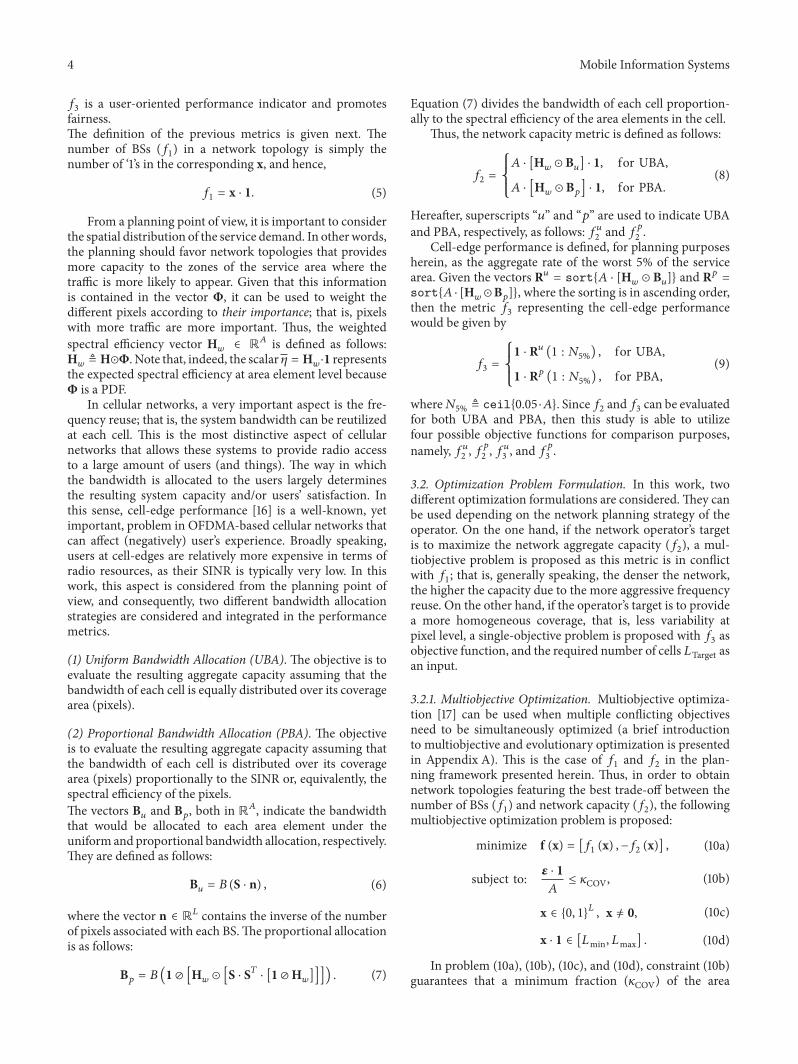
Therefore, to contextualize the proposed UDN planningand optimization framework in a realistic setting, we considera case study for UDN in a high-density urban settlement. Tothat end, we use the Hanna Nassif ward in Dar es Salaam,Tanzania, as the planning study case. Hanna Nassif hasan estimated population density of 40000 people/km2. Theapproximately 1 km2HannaNassif area includes around 3000buildings (mostly 3–6m tall) and is located on a terrainwith a topographical difference of 19m. A three-dimensional(3D) representation of this scenario is shown in Figure 1. Weassume that all candidate locations (indicated in white-bluedots) are outdoor at rooftop level. Rooftop deployed shared-access small cells provide improved outdoor coverage com-pared to indoor deployed small cells and enable line-of-sight(LOS) or near LOS (nLOS) conditions for the implementationof high-capacity wireless backhauling [25]. Moreover, therooftop is also a convenient location for off-grid operationof the small cells through energy harvesting from ambientrenewable energy sources (solar, wind, etc.) [26].

4.2. Parameters and Assumptions. The radio coverage esti-mations are based on realistic 3D building vectors andtopographical data (see Figure 1, for the simulation area)


dIS

Service area

700

m

500m

Topography (m)

18

14

10

6

2

dIS = 30m

Candidate location

Figure 1: The visualisation of the 3D buildings and topography of the planning case study deployment scenario. The candidate locations forthe UDN small cells are depicted with solid blue-white dots.

Table 1: Evaluation setting and parameters.

General settingCandidate locations(𝐿) 368 Carrier freq. 2.6GHz Bandwidth (𝐵) 20MHz

Building material Brick, 10 cm Number of pixels 350000 Number of PRBs 100Max. BS transmitpower (𝑃𝑛Txmax)

30 dBm Pixels’ resolution 1 × 1m2 Path loss WinProp ray tracing[27]

BS’s height 7m Noise power (𝜎2) −174 dBm/Hz Shadowing N(0.4) [dB]Cell selection (𝑓𝑐)

One server/highestRx. power Rx. power (𝑃min) −126 dBm Small scale fad. As in [28]

Link performance(𝑓LP)

Shannon’s formula Cov. (𝜅COV) 0.02 (2%) [𝐿min, 𝐿max] [180, 220] , [165, 195]

Max. path loss (𝐺ULmin) −163.40 dB Antenna pattern Omnidirectional 𝐿Target 180

Spatial userdistribution Uniform SINR (𝛾min) −10.0 dB — —

Calibration of NSGA-IIPopulation size 100 Crossover prob. 1.00 Type of var. DiscreteMutation prob. 1/𝐿 Termination crit. Hypervolume < 0.001%, [17]

and are evaluated using the deterministic dominant pathmodel implemented in the WinProp propagation modelingtool [27]. The simulation parameters and assumptions followthe IMT-Advanced guidelines [28] and are listed in Table 1.The building penetration losses are modeled explicitly toaccount for the outdoor-to-indoor propagation and it isassumed that all buildings outer walls are based on onematerial (10 cm brick) and in-building losses (e.g., due tointernal walls, doors) are approximated by an exponentialdecaymodel. Furthermore, as noted previously, the case studyarea includes a large number of densely packed small houses

or buildings of relatively low height built on a land withsignificant topographical differences over short distances.The deployment of rooftop smalls in this environment createssignificant multipath propagation, waveguiding effects, andoutdoor-to-indoor propagation that can be suitably capturedby a ray-tracing tool like WinProp (see, e.g., [29]). Indeed,it is noted that ray tracing provides significant accuracyimprovements compared to classicalmodels butwith reducedgenerality in terms of scenario selection [30]. The precision(pixel resolution) and inclusion of time-varying nonstation-ary objects (e.g., cars, pedestrians) may further influence


Service area

700

m

500m

×10−5

10

8

6

4

Pixe

l pro

babi

lity

(a) Nonuniform service demand distributionmap(Φ)

P(x

<Φ

)

1.0

0.8

0.6

0.4

0.2

0.0

Pixel probability (Φ)2 4 6 8 10 12

×10−5

Nonuniform service demand distributionUniform service demand distribution

(b) CDF ofΦ

Figure 2: Nonuniform service demand distribution used in numerical evaluations.

accuracy and computational effort of different ray-tracingcomputations. To that end, the pixel resolution in our studyis 1 × 1m2, which provides the right trade-off between mod-eling accuracy and feasible computational time. However,in WinProp environment we do not include the scatteringeffects of nonstationary objects for the sake of simplicity incapturing the scenario. Moreover, the usage of same ray-tracing path loss results for all topologies considered in thestudy ensures that the absolute accuracy of the ray tracingdoes not influence the performance comparisons between thetopologies. The parameters for the calibration of the NSGA-II algorithm are also shown inTable 1. Calibration parametersand complexity aspects are provided in Section 5.4.

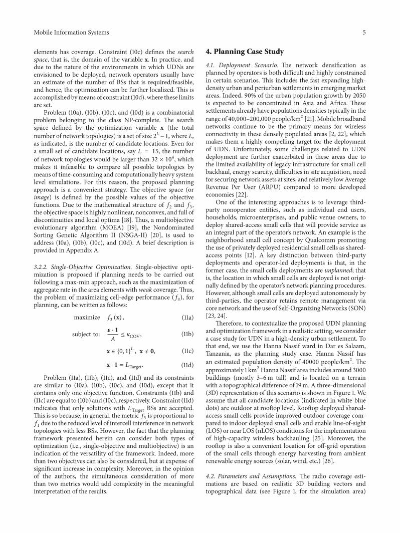
4.3. Spatial Traffic Distributions. Two different spatial trafficdistributions have been considered for the numerical evalua-tions presented in the next section: uniform and nonuniform.Uniform STD implies that the service demand is uniformlydistributed in the coverage area. Nonuniform STD impliesthat the traffic is more likely to appear in certain areas(hotspots), which is representative of how traffic is commonlydistributed in practice. The system model and optimizationframework presented herein are able to consider any arbitrarySTD bymeans of the vectorΦ, as it is explained in Section 3.1.Figure 2 shows a representation of the nonuniform STD usedin numerical evaluations. A 2-dimensional representation(map) is provided in Figure 2(a), where red areas correspondto hotspots. Figure 2(b) shows the CDF of the probability atpixel level in order to provide a perspective of the level ofirregularity of the nonuniform STD.The uniform STD is alsoindicated by the vertical dashed line. This input, as it will beseen shortly, has a profound impact on the optimization pro-cess and leads to significantly different network topologies.

4.4. Benchmarks. In order to clarify themerit of the proposedoptimization framework, several benchmarks have been con-sidered.

(1) Random Deployments. As explained earlier, open-accessoutdoor small cells (randomly deployed by users) wouldprovide a sustainable (cost efficient) approach to networkdensification. Thus, random topologies (located at candidatelocations) are considered.

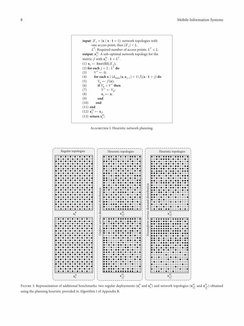
(2) Regular Deployments. Regularly deployed access points,that is, geometrically regular cells, are the natural choice foruniform STD and are often considered as a baseline. Tworegular topologies (x𝑅1 and x𝑅2 ) are considered and are shownin Figure 3.

(3) Heuristic Network Planning. A basic heuristic networkplanning for small cells is also considered.The correspondingpseudocode (Algorithm 1) and its explanation are provided inAppendix B. The resulting network topologies (x𝐻𝑓𝑢2 and x𝐻

𝑓𝑝

2

)from the heuristic algorithm are also shown in Figure 3 (bothfor uniform and nonuniform STD).

5. Numerical Results

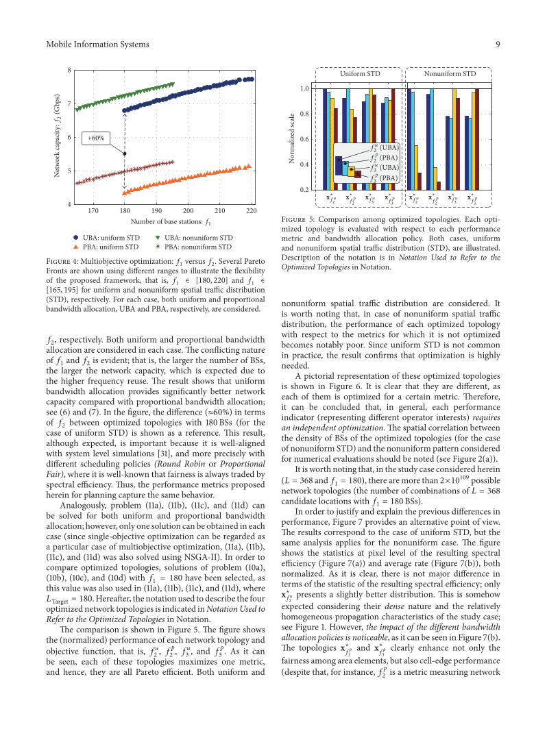
5.1. Optimization for Planning. Thesolution ofmultiobjectiveoptimization problems, such as (10a), (10b), (10c), and (10d),is a set of network topologies, all them featuring Paretoefficiency with respect to the objective functions, in this case𝑓1 and 𝑓2. The image of this set is called Pareto Front (seeAppendixA), and it is shown in Figure 4 for both uniformandnonuniform spatial traffic distribution, using different targetranges for 𝑓1. The 𝑥- and 𝑦-axes indicate the values of 𝑓1 and


input:X1 = {x | x ⋅ 1 = 1}: network topologies withone access point, thus |X1| = 𝐿.𝐿𝑇: Required number of access points. 𝐿𝑇 ≤ 𝐿.

output: x𝐻𝑓 : A sub-optimal network topology for themetric 𝑓 with x𝐻𝑓 ⋅ 1 = 𝐿𝑇.(1) x1 ← BestBS(X1);(2) for each 𝑗 = 2 : 𝐿𝑇 do(3) 𝑉⋆ ← 0;(4) for each x | (𝑑Ham(x, x𝑗−1) = 1)⋀(x ⋅ 1 = 𝑗) do(5) 𝑉x ← 𝑓(x);(6) if 𝑉x > 𝑉⋆ then(7) 𝑉⋆ ← 𝑉x;(8) x𝑗 ← x;(9) end(10) end(11) end(12) x𝐻𝑓 ← x𝑗;(13) return x𝐻𝑓 ;

Algorithm 1: Heuristic network planning.

Regular topologies Heuristic topologies Heuristic topologies

Uniform

serv

ice d

eman

d di

strib

utio

n

Nonu

niform

serv

ice d

eman

d di

strib

utio

n

xR1

xR2

xHfu2

xH

xHfu2

xHfp2 f

p2

Figure 3: Representation of additional benchmarks: two regular deployments (x𝑅1 and x𝑅2 ) and network topologies (x𝐻𝑓𝑢2and x𝐻

𝑓𝑝

2

) obtainedusing the planning heuristic provided in Algorithm 1 of Appendix B.

Mobile Information Systems 9N

etw

ork

capa

city

:f2

(Gbp

s)

8

7

6

5

4

Number of base stations: f1

170 180 190 200 210 220

+60%

UBA: uniform STDPBA: uniform STD

UBA: nonuniform STDPBA: nonuniform STD

Figure 4: Multiobjective optimization: 𝑓1 versus 𝑓2. Several ParetoFronts are shown using different ranges to illustrate the flexibilityof the proposed framework, that is, 𝑓1 ∈ [180, 220] and 𝑓1 ∈[165, 195] for uniform and nonuniform spatial traffic distribution(STD), respectively. For each case, both uniform and proportionalbandwidth allocation, UBA and PBA, respectively, are considered.

𝑓2, respectively. Both uniform and proportional bandwidthallocation are considered in each case. The conflicting natureof 𝑓1 and 𝑓2 is evident; that is, the larger the number of BSs,the larger the network capacity, which is expected due tothe higher frequency reuse. The result shows that uniformbandwidth allocation provides significantly better networkcapacity compared with proportional bandwidth allocation;see (6) and (7). In the figure, the difference (≈60%) in termsof 𝑓2 between optimized topologies with 180 BSs (for thecase of uniform STD) is shown as a reference. This result,although expected, is important because it is well-alignedwith system level simulations [31], and more precisely withdifferent scheduling policies (Round Robin or ProportionalFair), where it is well-known that fairness is always traded byspectral efficiency. Thus, the performance metrics proposedherein for planning capture the same behavior.

Analogously, problem (11a), (11b), (11c), and (11d) canbe solved for both uniform and proportional bandwidthallocation; however, only one solution can be obtained in eachcase (since single-objective optimization can be regarded asa particular case of multiobjective optimization, (11a), (11b),(11c), and (11d) was also solved using NSGA-II). In order tocompare optimized topologies, solutions of problem (10a),(10b), (10c), and (10d) with 𝑓1 = 180 have been selected, asthis value was also used in (11a), (11b), (11c), and (11d), where𝐿Target = 180. Hereafter, the notation used to describe the fouroptimized network topologies is indicated inNotationUsed toRefer to the Optimized Topologies in Notation.

The comparison is shown in Figure 5. The figure showsthe (normalized) performance of each network topology andobjective function, that is, 𝑓𝑢2 , 𝑓

𝑝2 , 𝑓𝑢3 , and 𝑓𝑝3 . As it can

be seen, each of these topologies maximizes one metric,and hence, they are all Pareto efficient. Both uniform and

Uniform STD Nonuniform STD

Nor

mal

ized

scal

e

1.0

0.8

0.6

0.4

0.2x⋆fu

2x⋆fp2

x⋆fu3

x⋆fp3

x⋆fu2

x⋆fp2

x⋆fu3

x⋆fp3

fu2 (UBA)

fp2 (PBA)

fu3 (UBA)

fp3 (PBA)

Figure 5: Comparison among optimized topologies. Each opti-mized topology is evaluated with respect to each performancemetric and bandwidth allocation policy. Both cases, uniformand nonuniform spatial traffic distribution (STD), are illustrated.Description of the notation is in Notation Used to Refer to theOptimized Topologies in Notation.

nonuniform spatial traffic distribution are considered. Itis worth noting that, in case of nonuniform spatial trafficdistribution, the performance of each optimized topologywith respect to the metrics for which it is not optimizedbecomes notably poor. Since uniform STD is not commonin practice, the result confirms that optimization is highlyneeded.

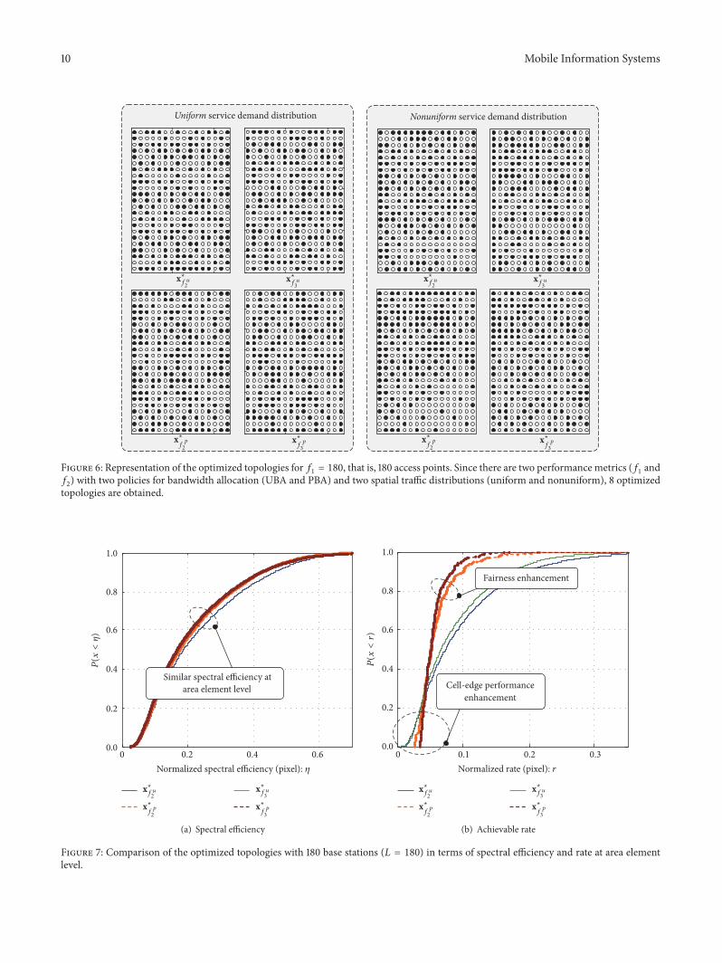
A pictorial representation of these optimized topologiesis shown in Figure 6. It is clear that they are different, aseach of them is optimized for a certain metric. Therefore,it can be concluded that, in general, each performanceindicator (representing different operator interests) requiresan independent optimization. The spatial correlation betweenthe density of BSs of the optimized topologies (for the caseof nonuniform STD) and the nonuniform pattern consideredfor numerical evaluations should be noted (see Figure 2(a)).

It is worth noting that, in the study case considered herein(𝐿 = 368 and𝑓1 = 180), there aremore than 2×10109 possiblenetwork topologies (the number of combinations of 𝐿 = 368candidate locations with 𝑓1 = 180BSs).

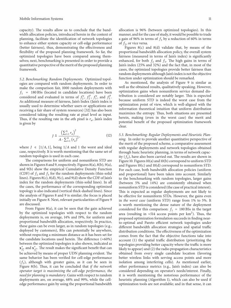
In order to justify and explain the previous differences inperformance, Figure 7 provides an alternative point of view.The results correspond to the case of uniform STD, but thesame analysis applies for the nonuniform case. The figureshows the statistics at pixel level of the resulting spectralefficiency (Figure 7(a)) and average rate (Figure 7(b)), bothnormalized. As it is clear, there is not major difference interms of the statistic of the resulting spectral efficiency; onlyx⋆𝑓𝑢2 presents a slightly better distribution. This is somehowexpected considering their dense nature and the relativelyhomogeneous propagation characteristics of the study case;see Figure 1. However, the impact of the different bandwidthallocation policies is noticeable, as it can be seen in Figure 7(b).The topologies x⋆

𝑓𝑝

2

and x⋆𝑓𝑝

3

clearly enhance not only thefairness among area elements, but also cell-edge performance(despite that, for instance, 𝑓𝑝2 is a metric measuring network


Uniform service demand distribution Nonuniform service demand distribution

x⋆fu2

x⋆f

p2

x⋆fu3

x⋆fu2

x⋆fu3

x⋆f

p3

x⋆f

p2

x⋆f

p3

Figure 6: Representation of the optimized topologies for𝑓1 = 180, that is, 180 access points. Since there are two performance metrics (𝑓1 and𝑓2) with two policies for bandwidth allocation (UBA and PBA) and two spatial traffic distributions (uniform and nonuniform), 8 optimizedtopologies are obtained.

P(x

<𝜂

)

1.0

0.8

0.6

0.4

0.2

0.0

Normalized spectral efficiency (pixel): 𝜂0 0.2 0.4 0.6

Similar spectral efficiency atarea element level

x⋆fu2

x⋆fu3

x⋆f

p2

x⋆f

p3

(a) Spectral efficiency

1.0

0.8

0.6

0.4

0.2

0.0

Normalized rate (pixel): r

P(x

<r)

Fairness enhancement

Cell-edge performanceenhancement

0 0.1 0.2 0.3

x⋆fu2

x⋆fu3

x⋆f

p2

x⋆f

p3

(b) Achievable rate

Figure 7: Comparison of the optimized topologies with 180 base stations (𝐿 = 180) in terms of spectral efficiency and rate at area elementlevel.


capacity). The results allow us to conclude that the band-width allocation policies, introduced herein in the context ofplanning, facilitate the identification of network topologiesto enhance either system capacity or cell-edge performance(better fairness), thus, demonstrating the effectiveness andflexibility of the proposed planning framework. So far, theoptimized topologies have been compared among them-selves; next, benchmarking is presented in order to provide aquantitative perspective of themerit of the proposed planningframework.

5.2. Benchmarking: Random Deployments. Optimized topol-ogies are compared with random deployments. In order tomake the comparison fair, 1000 random deployments with𝑓1 = 180BSs (located in candidate locations) have beenconsidered and evaluated in terms of 𝑓𝑢2 , 𝑓

𝑝2 , 𝑓𝑢3 , and 𝑓𝑝3 .

As additional measure of fairness, Jain’s Index (Jain’s index isusually used to determine whether users or applications arereceiving a fair share of system resources) [32] has also beenconsidered taking the resulting rate at pixel level as input.Thus, if the resulting rate in the 𝑎th pixel is 𝑟𝑎, Jain’s indexis given by

𝐽 ≜(∑𝐴𝑖=1 𝑟𝑎)

2

𝐴 ⋅ ∑𝐴𝑖=1 (𝑟𝑎)2, (12)

where 𝐽 ∈ [1/𝐴, 1], being 1/𝐴 and 1 the worst and idealcase, respectively. It is worth mentioning that the same set ofrandom topologies is used in each case.

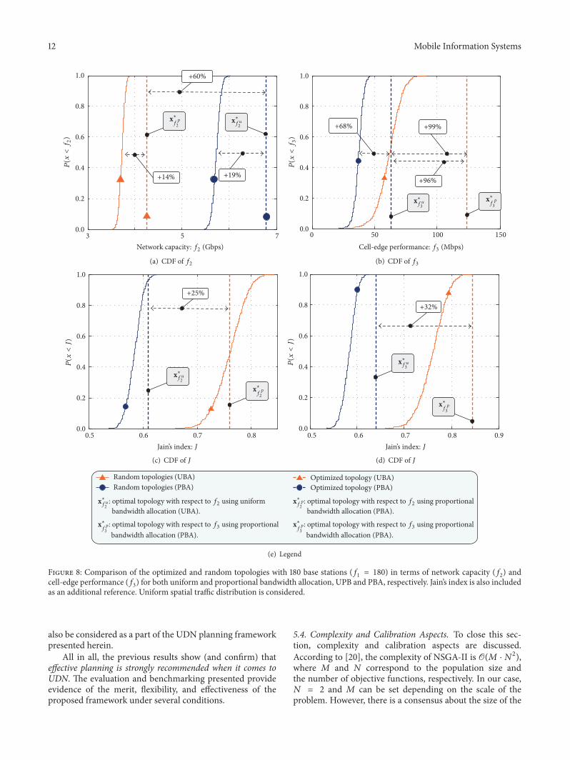
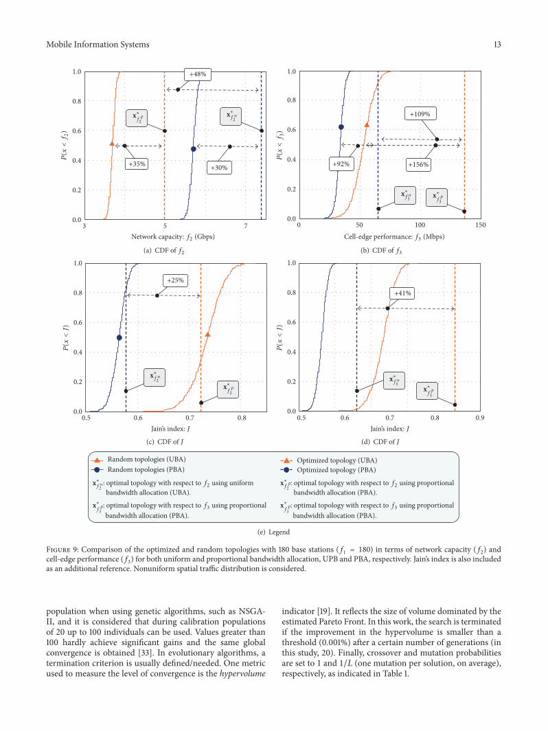
The comparisons for uniform and nonuniform STD areshown in Figures 8 and 9, respectively. Figures 8(a), 8(b), 9(a),and 9(b) show the empirical Cumulative Density Function(CDF) of 𝑓2 and 𝑓3 for the random deployments (thin-solidlines). Figures 8(c), 8(d), 9(c), and 9(d) show the CDF of Jain’sindex for the random deployments (thin-solid lines). In allthe cases, the performance of the corresponding optimizedtopology is also indicated (vertical thick-dashed lines). Sincethe analysis of Figures 8 and 9 is similar; the focus is placedinitially on Figure 8. Next, relevant particularities of Figure 9are discussed.

From Figure 8(a), it can be seen that the gain achievedby the optimized topologies with respect to the randomdeployments is, on average, 14% and 19%, for uniform andproportional bandwidth allocation, respectively. In practice,these gains can be even larger, as in random topologies (e.g.,deployed by customers), BSs can potentially be anywhere,without respecting a minimum distance as it has been set forthe candidate locations used herein. The difference (≈60%)between the optimized topologies is also shown, indicated asx⋆𝑓𝑢2 and x⋆

𝑓𝑝

2

. The result makes the significant benefit that canbe achieved by means of proper UDN planning evident. Thesame behavior has been verified for cell-edge performance(𝑓3), although with greater gains, as it can be seen inFigure 8(b). Thus, it can be concluded that if the networkoperator target is maximizing the cell-edge performance, theneed for planning is mandatory. Gains with respect to randomdeployments are, on average, 68% and 99%, while the cell-edge performance gain by using the proportional bandwidth

allocation is 96% (between optimized topologies). In thismanner, and for the case of study, it would be possible to tradea gain of 96% in terms of 𝑓3 by a reduction of 60% in termsof 𝑓2, or vice versa.

Figures 8(c) and 8(d) validate that, by means of theproportional bandwidth allocation policy, the overall systemfairness (measured in terms of Jain’s index) is significantlyenhanced, for both 𝑓2 and 𝑓3. The high gains in terms ofJain’s index (25% and 32%) and the fact that, in most of thecases, the optimized topologies provide better fairness thanrandomdeployments although Jain’s index is not the objectivefunction under optimization should be remarked.

As mentioned, the analysis of Figure 9 is similar aswell as the obtained results, qualitatively speaking. However,optimization gains when nonuniform service demand dis-tribution is considered are notably larger. This is expectedbecause uniform STD is indeed the worst case from theoptimization point of view, which is well-aligned with theinformation theoretical intuition that uniform distributionmaximizes the entropy. Thus, both situations are presentedherein, making (even in the worst case) the merit andpotential benefit of the proposed optimization frameworkclear.

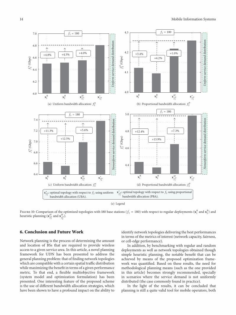
5.3. Benchmarking: Regular Deployments and Heuristic Plan-ning. In order to provide another quantitative perspective ofthe merit of the proposed scheme, a comparative assessmentwith regular deployments and network topologies obtainedthrough basic heuristic planning, in terms of network capac-ity (𝑓2), have also been carried out. The results are shown inFigure 10. Figures 10(a) and 10(b) correspond to uniform STDand Figures 10(c) and 10(d) correspond to nonuniform STD.For each case, both bandwidth allocation policies (uniformand proportional) have been taken into account. Similarlyto the benchmarking with random topologies, larger gains(between 5% and 14%) are consistently obtained whennonuniform STD is considered (the case of practical interest).This is expected as regular deployments are not likely tobe effective for nonuniform STDs. However, the gains evenin the worst case (uniform STD) range from 1% to 5%. Itis worth mentioning the dense nature of the deploymentconsidered for this comparison: 𝑓1 = 180BSs in the targetarea (resulting in ≈514 access points per km2). Thus, theproposed optimization formulation succeeds in finding near-to-optimal and Pareto efficient network topologies underdifferent bandwidth allocation strategies and spatial trafficdistribution conditions.The effectiveness of the optimizationcomes from the fact that the objective functions take intoaccount (1) the spatial traffic distribution (prioritizing thetopologies providing better capacity where the traffic is morelikely to appear) and (2) the radio propagation characteristicsobtained from every single candidate location (favoringbetter wireless links with serving access points and moreisolation among interfering cells). As mentioned earlier,other performance metrics (e.g., Jain’s index) can also beconsidered depending on operator’s needs/interest. Finally,it is worth mentioning the notorious performance of theheuristic planning (Algorithm 1), which can also be used ifoptimization tools are not available; and in that sense, it can


+60%

+14% +19%

x⋆fu2

x⋆fp2

P(x

<f2)

1.0

0.8

0.6

0.4

0.2

0.0

Network capacity: f2 (Gbps)3 5 7

(a) CDF of 𝑓2

+68% +99%

+96%

x⋆f

p3

1.0

0.8

0.6

0.4

0.2

0.0

x⋆fu3

Cell-edge performance: f3 (Mbps)0 50 100 150

P(x

<f3)

(b) CDF of 𝑓3

+25%

x⋆fu2

x⋆f

p2

1.0

0.8

0.6

0.4

0.2

0.0

P(x

<J)

Jain’s index: J0.5 0.6 0.7 0.8

(c) CDF of 𝐽

+32%

1.0

0.8

0.6

0.4

0.2

0.0

x⋆fu3

x⋆f

p3

P(x

<J)

Jain’s index: J0.5 0.6 0.7 0.8 0.9

(d) CDF of 𝐽

Random topologies (UBA)Random topologies (PBA)

Optimized topology (UBA)Optimized topology (PBA)

x⋆fu2

: optimal topology with respect to f2 using uniformbandwidth allocation (UBA).

x⋆fp3

: optimal topology with respect to f3 using proportionalbandwidth allocation (PBA).

x⋆fp2


x⋆fp3


(e) Legend

Figure 8: Comparison of the optimized and random topologies with 180 base stations (𝑓1 = 180) in terms of network capacity (𝑓2) andcell-edge performance (𝑓3) for both uniform and proportional bandwidth allocation, UPB and PBA, respectively. Jain’s index is also includedas an additional reference. Uniform spatial traffic distribution is considered.

also be considered as a part of the UDN planning frameworkpresented herein.

All in all, the previous results show (and confirm) thateffective planning is strongly recommended when it comes toUDN. The evaluation and benchmarking presented provideevidence of the merit, flexibility, and effectiveness of theproposed framework under several conditions.

5.4. Complexity and Calibration Aspects. To close this sec-tion, complexity and calibration aspects are discussed.According to [20], the complexity of NSGA-II is O(𝑀 ⋅ 𝑁2),where 𝑀 and 𝑁 correspond to the population size andthe number of objective functions, respectively. In our case,𝑁 = 2 and 𝑀 can be set depending on the scale of theproblem. However, there is a consensus about the size of the


+35% +30%

+48%

x⋆fu2

x⋆f

p2

P(x

<f2)

1.0

0.8

0.6

0.4

0.2

0.0

Network capacity: f2 (Gbps)3 5 7

(a) CDF of 𝑓2

+109%

+156%+92%

x⋆fu3

x⋆fp3

1.0

0.8

0.6

0.4

0.2

0.0

Cell-edge performance: f3 (Mbps)0 50 100 150

P(x

<f3)

(b) CDF of 𝑓3

+25%

x⋆fu2

x⋆f

p2

1.0

0.8

0.6

0.4

0.2

0.0

P(x

<J)

Jain’s index: J0.5 0.6 0.7 0.8

(c) CDF of 𝐽

+41%

x⋆fu3

x⋆f

p3

1.0

0.8

0.6

0.4

0.2

0.0

P(x

<J)

Jain’s index: J0.5 0.6 0.7 0.8 0.9

(d) CDF of 𝐽

Random topologies (UBA)Random topologies (PBA)

Optimized topology (UBA)Optimized topology (PBA)

x⋆fu2


x⋆f

p3


x⋆fp2


x⋆f

p3


(e) Legend

Figure 9: Comparison of the optimized and random topologies with 180 base stations (𝑓1 = 180) in terms of network capacity (𝑓2) andcell-edge performance (𝑓3) for both uniform and proportional bandwidth allocation, UPB and PBA, respectively. Jain’s index is also includedas an additional reference. Nonuniform spatial traffic distribution is considered.

population when using genetic algorithms, such as NSGA-II, and it is considered that during calibration populationsof 20 up to 100 individuals can be used. Values greater than100 hardly achieve significant gains and the same globalconvergence is obtained [33]. In evolutionary algorithms, atermination criterion is usually defined/needed. One metricused to measure the level of convergence is the hypervolume

indicator [19]. It reflects the size of volume dominated by theestimated Pareto Front. In this work, the search is terminatedif the improvement in the hypervolume is smaller than athreshold (0.001%) after a certain number of generations (inthis study, 20). Finally, crossover and mutation probabilitiesare set to 1 and 1/𝐿 (one mutation per solution, on average),respectively, as indicated in Table 1.


fu 2

(Gbp

s)7.0

6.8

6.6

6.4

6.2

6.0

f1 = 180

+4.8% +4.5% +4.0%

xR1 xR

2 xHfu2

x⋆fu2

Uniform

serv

ice d

eman

d di

strib

utio

n

(a) Uniform bandwidth allocation: 𝑓𝑢2

f1 = 180

+3.4%+4.2%

+1.0%

fp 2

(Gbp

s)

4.3

4.2

4.1

4.0

xR1 xR2 x⋆fp2

xHfp2

Uniform

serv

ice d

eman

d di

strib

utio

n

(b) Proportional bandwidth allocation: 𝑓𝑝2

xR1 xR2 xHfu2

x⋆fu2

fu 2

(Gbp

s)

7.4

7.2

7.0

6.8

6.6

6.4

f1 = 180

+11.3%

+12.5%

+5.6%

Nonu

niform

serv

ice d

eman

d di

strib

utio

n

(c) Uniform bandwidth allocation: 𝑓𝑢2

xR1 xR

2

fu 2

(Gbp

s)

5.0

4.8

4.6

4.4

f1 = 180

+12.4%

+13.9%

+7.3%

x⋆f

p2

xHf

p2

Nonu

niform

serv

ice d

eman

d di

strib

utio

n

(d) Proportional bandwidth allocation: 𝑓𝑝2

x⋆f

p2


x⋆fu2


(e) Legend

Figure 10: Comparison of the optimized topologies with 180 base stations (𝑓1 = 180) with respect to regular deployments (x𝑅1 and x𝑅2 ) andheuristic planning (x𝐻𝑓𝑢

2and x𝐻

𝑓𝑝

2

).

6. Conclusion and Future Work

Network planning is the process of determining the amountand location of BSs that are required to provide wirelessaccess to a given service area. In this article, a novel planningframework for UDN has been presented to address thegeneral planning problem: that of finding network topologieswhich are compatible with a certain spatial traffic distributionwhilemaximizing the benefit in terms of a given performancemetric. To that end, a flexible multiobjective framework(system model and optimization formulation) has beenpresented. One interesting feature of the proposed schemeis the use of different bandwidth allocation strategies, whichhave been shown to have a profound impact on the ability to

identify network topologies delivering the best performancesin terms of the metrics of interest (network capacity, fairness,or cell-edge performance).

In addition, by benchmarking with regular and randomdeployments as well as network topologies obtained thoughsimple heuristic planning, the notable benefit that can beachieved by means of the proposed optimization frame-work was quantified. Based on these results, the need formethodological planning means (such as the one providedin this article) becomes strongly recommended, speciallyin scenarios where the service demand is not uniformlydistributed (the case commonly found in practice).

In the light of the results, it can be concluded thatplanning is still a quite valid tool for mobile operators, both


Obj

ectiv

e1

Objective 2

Dominated solutions

Pareto Front(nondominated solutions)

Figure 11: Pictorial representation of a Pareto Front.

nowadays and in future 5G systems, where small cells areof utmost importance. The framework studied herein is richand admits several future research directions. Consideringadditional objective functions is definitely a study item, aswell as other optimization formulations that could be specificfor certain use cases, such as Downlink Uplink Decoupling.In addition, upgrading fixed/existing deployments is of greatpractical interest, as well as adaptation of coverage patterns,and power optimization. Finally, planning studies for UDNoperating at higher frequency bands is also on our roadmap.

Appendix

A. Multiobjective and EvolutionaryOptimization

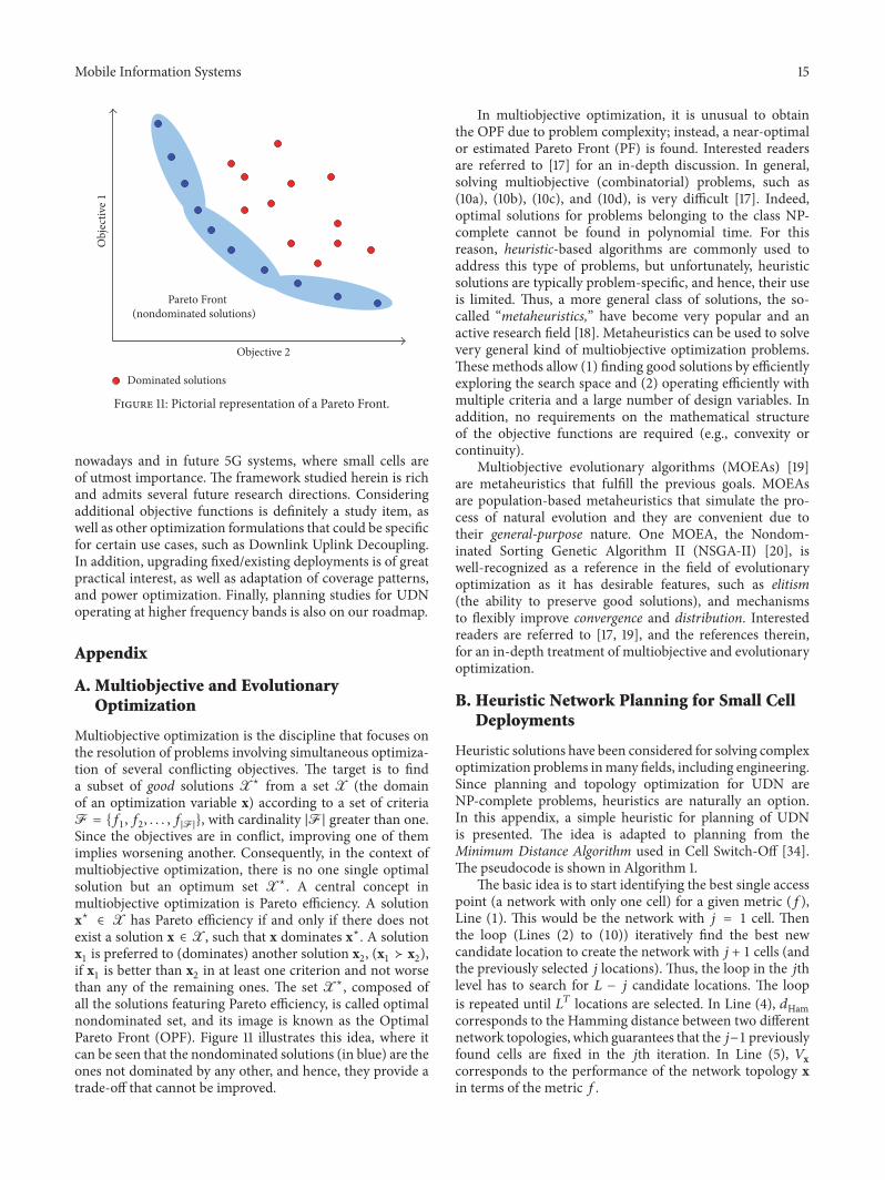
Multiobjective optimization is the discipline that focuses onthe resolution of problems involving simultaneous optimiza-tion of several conflicting objectives. The target is to finda subset of good solutions X⋆ from a set X (the domainof an optimization variable x) according to a set of criteriaF = {𝑓1, 𝑓2, . . . , 𝑓|F|}, with cardinality |F| greater than one.Since the objectives are in conflict, improving one of themimplies worsening another. Consequently, in the context ofmultiobjective optimization, there is no one single optimalsolution but an optimum set X⋆. A central concept inmultiobjective optimization is Pareto efficiency. A solutionx⋆ ∈ X has Pareto efficiency if and only if there does notexist a solution x ∈ X, such that x dominates x⋆. A solutionx1 is preferred to (dominates) another solution x2, (x1 ≻ x2),if x1 is better than x2 in at least one criterion and not worsethan any of the remaining ones. The set X⋆, composed ofall the solutions featuring Pareto efficiency, is called optimalnondominated set, and its image is known as the OptimalPareto Front (OPF). Figure 11 illustrates this idea, where itcan be seen that the nondominated solutions (in blue) are theones not dominated by any other, and hence, they provide atrade-off that cannot be improved.

In multiobjective optimization, it is unusual to obtainthe OPF due to problem complexity; instead, a near-optimalor estimated Pareto Front (PF) is found. Interested readersare referred to [17] for an in-depth discussion. In general,solving multiobjective (combinatorial) problems, such as(10a), (10b), (10c), and (10d), is very difficult [17]. Indeed,optimal solutions for problems belonging to the class NP-complete cannot be found in polynomial time. For thisreason, heuristic-based algorithms are commonly used toaddress this type of problems, but unfortunately, heuristicsolutions are typically problem-specific, and hence, their useis limited. Thus, a more general class of solutions, the so-called “metaheuristics,” have become very popular and anactive research field [18]. Metaheuristics can be used to solvevery general kind of multiobjective optimization problems.These methods allow (1) finding good solutions by efficientlyexploring the search space and (2) operating efficiently withmultiple criteria and a large number of design variables. Inaddition, no requirements on the mathematical structureof the objective functions are required (e.g., convexity orcontinuity).

Multiobjective evolutionary algorithms (MOEAs) [19]are metaheuristics that fulfill the previous goals. MOEAsare population-based metaheuristics that simulate the pro-cess of natural evolution and they are convenient due totheir general-purpose nature. One MOEA, the Nondom-inated Sorting Genetic Algorithm II (NSGA-II) [20], iswell-recognized as a reference in the field of evolutionaryoptimization as it has desirable features, such as elitism(the ability to preserve good solutions), and mechanismsto flexibly improve convergence and distribution. Interestedreaders are referred to [17, 19], and the references therein,for an in-depth treatment of multiobjective and evolutionaryoptimization.

B. Heuristic Network Planning for Small CellDeployments

Heuristic solutions have been considered for solving complexoptimization problems inmany fields, including engineering.Since planning and topology optimization for UDN areNP-complete problems, heuristics are naturally an option.In this appendix, a simple heuristic for planning of UDNis presented. The idea is adapted to planning from theMinimum Distance Algorithm used in Cell Switch-Off [34].The pseudocode is shown in Algorithm 1.

The basic idea is to start identifying the best single accesspoint (a network with only one cell) for a given metric (𝑓),Line (1). This would be the network with 𝑗 = 1 cell. Thenthe loop (Lines (2) to (10)) iteratively find the best newcandidate location to create the network with 𝑗 + 1 cells (andthe previously selected 𝑗 locations). Thus, the loop in the 𝑗thlevel has to search for 𝐿 − 𝑗 candidate locations. The loopis repeated until 𝐿𝑇 locations are selected. In Line (4), 𝑑Hamcorresponds to the Hamming distance between two differentnetwork topologies, which guarantees that the 𝑗−1 previouslyfound cells are fixed in the 𝑗th iteration. In Line (5), 𝑉xcorresponds to the performance of the network topology xin terms of the metric 𝑓.


Notation

Basic Notation

𝐵: System bandwidth𝐿: Number of candidate locations𝐴: Number of area elementsG: Channel gain matrix𝑃min: Target received power𝐺ULmin: Minimum channel gainΦ: Spatial demand distributionH: Spectral efficiency vectorΓ: Average SINR vectorn: Inverse of cell’s size𝑃max: Maximum transmit power per cellA: Set of area elements in the target areaRRS: Received power matrixpPS, p𝐷: Power vectors: pilots and data channelsx: Network topologyA𝑙: Coverage of the 𝑙th BSS, S𝑐: Coverage matrices𝛾min: Minimum SINR𝜀: Coverage vector𝜅COV: Coverage threshold

Notation Used to Refer to the Optimized Topologies

x⋆𝑓𝑢2 : Optimal topology with respect to 𝑓2 usinguniform bandwidth allocation (UBA)

x⋆𝑓𝑝

2

: Optimal topology with respect to 𝑓2 usingproportional bandwidth allocation (PBA)

x⋆𝑓𝑢3 : Optimal topology with respect to 𝑓3 usinguniform bandwidth allocation (UBA)

x⋆𝑓𝑝

3

: Optimal topology with respect to 𝑓3 usingproportional bandwidth allocation (PBA).

Competing Interests

The authors declare that there is no conflict of interestsregarding the publication of this paper.

Acknowledgments

Hanna Nassif GIS data was kindly provided by Professor R.Sliuzas of ITC-Faculty of Geo-Information Science & EarthObservation, University of Twente. This work is partiallysupported by the Academy of Finland under Grants 287249and 284634. Furthermore, this work received partial supportfrom the National Bureau of Science, Technology and Inno-vation of Panama (SENACYT) through the project RAPIDO(ITE15-021).

References

[1] Nokia, Ultra dense network (UDN) white paper. Nokia Solu-tions andNeworksOy, June 2016, http://resources.alcatel-lucent.com/asset/200295.

[2] Ericsson, Ericsson mobility report: on the pulse of the net-worked society, June 2016, https://www.ericsson.com/res/docs/2016/ericssonmobility-report-2016.pdf.

[3] J. Zander and P. Mahonen, “Riding the data tsunami in thecloud: myths and challenges in future wireless access,” IEEECommunications Magazine, vol. 51, no. 3, pp. 145–151, 2013.

[4] I. Hwang, B. Song, and S. Soliman, “A holistic view on hyper-dense heterogeneous and small cell networks,” IEEE Communi-cations Magazine, vol. 51, no. 6, pp. 20–27, 2013.

[5] D. Lopez-Perez, M. Ding, H. Claussen, and A. H. Jafari,“Towards 1 Gbps/UE in cellular systems: understanding ultra-dense small cell deployments,” IEEE Communications Surveysand Tutorials, vol. 17, no. 4, pp. 2078–2101, 2015.

[6] Small Cell Forum (SCF), “Small cells—what is the big idea?Small Cell Forum,” February, 2012 http://scf.io/.

[7] X. Ge, S. Tu, G. Mao, C.-X. Wang, and T. Han, “5G ultra-densecellular networks,” IEEE Wireless Communications, vol. 23, no.1, pp. 72–79, 2016.

[8] H. Peng, Y. Xiao, Y.-N. Ruyue, and Y. Yifei, “Ultra densenetwork: challenges, enabling technologies and new trends,”China Communications, vol. 13, no. 2, Article ID 7405723, pp.30–40, 2016.

[9] W. Yu, H. Xu, H. Zhang, D. Griffith, and N. Golmie, “Ultra-dense networks: survey of state of the art and future directions,”in Proceedings of the 25th International Conference on ComputerCommunication and Networks (ICCCN ’16), pp. 1–10, Waikoloa,Hawaii, USA, August 2016.

[10] M. Kamel, W. Hamouda, and A. Youssef, “Ultra-dense net-works: a survey,” IEEECommunications Surveys&Tutorials, vol.18, no. 4, pp. 2522–2545, 2016.

[11] M. Jaber, Z. Dawy, N. Akl, and E. Yaacoub, “Tutorial onLTE/LTE-A cellular network dimensioning using iterative sta-tistical analysis,” IEEE Communications Surveys and Tutorials,vol. 18, no. 2, pp. 1355–1383, 2016.

[12] Qualcomm Research, “Neighborhood small cells for hyper-dense deployments: taking hetnets to the next level,” Tech.Rep., Qualcomm, San Diego, Calif, USA, 2013, https://www.qualcomm.com/.

[13] S.Wang andC. Ran, “Rethinking cellular network planning andoptimization,” IEEEWireless Communications, vol. 23, no. 2, pp.118–125, 2016.

[14] X. Zhou, Z. Zhao, R. Li, Y. Zhou, and H. Zhang, “Thepredictability of cellular networks traffic,” in Proceedings of theInternational Symposium on Communications and InformationTechnologies (ISCIT ’12), pp. 973–978, October 2012.

[15] I. Siomina and D. Yuan, “Analysis of cell load coupling forLTE network planning and optimization,” IEEE Transactions onWireless Communications, vol. 11, no. 6, pp. 2287–2297, 2012.

[16] G. D. Gonzalez, M. Garcia-Lozano, S. Ruiz Boque, and D.S. Lee, “Optimization of soft frequency reuse for irregularLTE macrocellular networks,” IEEE Transactions on WirelessCommunications, vol. 12, no. 5, pp. 2410–2423, 2013.

[17] Y. Sawaragi, H. Nakayama, and T. Tanino, Theory of Multi-objective Optimization, vol. 176 of Mathematics in Science andEngineering, Academic Press, Orlando, Fla, USA, 1st edition,1985.

[18] T. Weise, Global Optimization Algorithms&Theory and Applica-tion, 2nd edition, 2009, http://www.it-weise.de/.

[19] C. A. Coello Coello, G. B. Lamont, and D. A. Van Veldhuizen,Evolutionary algorithms for solving multi-objective problems,Genetic and Evolutionary Computation Series, Springer, NY,USA, Second edition, 2007.

[20] K. Deb, A. Pratap, S. Agarwal, and T. Meyarivan, “A fastand elitist multiobjective genetic algorithm: NSGA-II,” IEEE

http://resources.alcatel-lucent.com/asset/200295

http://resources.alcatel-lucent.com/asset/200295

https://www.ericsson.com/res/docs/2016/ericssonmobility-report-2016.pdf

https://www.ericsson.com/res/docs/2016/ericssonmobility-report-2016.pdf

http://scf.io/

https://www.qualcomm.com/

https://www.qualcomm.com/

http://www.it-weise.de/


Transactions on Evolutionary Computation, vol. 6, no. 2, pp. 182–197, 2002.

[21] UN, “World urbanization prospects: the 2014 revision,highlights,” UN Report ST/ESA/SER.A/352, United Nations,Department of Economic and Social Affairs, PopulationDivision, New York, NY, USA, 2014, https://esa.un.org/unpd/wup/Publications/Files/WUP2014-Highlights.pdf.

[22] GSMA, “The mobile economy Africa 2016,” 2016, http://www.gsma.com/mobileeconomy/africa/.

[23] H. Klessig, D. Ohmann, A. I. Reppas et al., “From immune cellsto self-organizing ultra-dense small cell networks,” IEEE Journalon Selected Areas in Communications, vol. 34, no. 4, pp. 800–811,2016.

[24] 3GPP, “Evolved Universal Terrestrial Radio Access Network (E-UTRAN); self-configuring and self-optimizing network (SON)use cases and solutions,” 3GPP Standard TR 36.902, 2011,http://www.3gpp.org/dynareport/36902.htm.

[25] P.Amin,N. S. Kibret, E.Mutafungwa, B. B.Haile, J.Hamalainen,and J. K. Nurminen, “Performance study for off-grid self-backhauled small cells in dense informal settlements,” in Pro-ceedings of the 25th IEEE Annual International Symposiumon Personal, Indoor, and Mobile Radio Communication (IEEEPIMRC ’14), pp. 1652–1657, September 2014.

[26] Y. Mao, Y. Luo, J. Zhang, and K. B. Letaief, “Energy harvestingsmall cell networks: Feasibility, deployment, and operation,”IEEE CommunicationsMagazine, vol. 53, no. 6, pp. 94–101, 2015.

[27] Altair, Winprop overview, http://www.altairhyperworks.com/product/FEKO/WinProp.

[28] ITU-R, “Guidelines for evaluation of radio interface technolo-gies for IMT-Advanced,” ITU Std. ITU-R, M.2135, 2008.

[29] L. Simic, J. Riihijarvi, and P. Mahonen, “Can statistical propa-gation models be saved by real 3D city data?: A RegionalizedStudy of Radio Coverage in New York City,” in Proceedings ofthe IEEE International Symposium on Dynamic Spectrum AccessNetworks (DySPAN ’15), pp. 285–288, October 2015.

[30] P. Ferrand, M. Amara, S. Valentin, and M. Guillaud, “Trendsand challenges in wireless channel modeling for evolving radioaccess,” IEEE Communications Magazine, vol. 54, no. 7, pp. 93–99, 2016.

[31] D. Gonzalez, S. Ruiz, M. Garcıa-Lozano, J. Olmos, and A. Serra,“System level evaluation of LTE networks with semidistributedintercell interference coordination,” in Proceedings of the IEEE20th International Symposium on Personal, Indoor and MobileRadio Communications, pp. 1497–1501, IEEE, Tokyo, Japan,September 2009.

[32] R. Jain, The Art of Computer Systems Performance Analysis:Techniques for Experimental Design, Measurement, Simulation,and Modeling, John Wiley & Sons, New York, NY, USA, 1990.

[33] J. C. Spall, Introduction to Stochastic Search and Optimization:Estimation, Simulation, and Control, vol. 65, JohnWiley & Sons,2005.

[34] D. G. Gonzalez, J. Hamalainen, H. Yanikomeroglu, M. Garcia-Lozano, and G. Senarath, “A novel multiobjective cell switch-offframework for cellular networks,” IEEE Access, vol. 4, pp. 7883–7898, 2016.

https://esa.un.org/unpd/wup/Publications/Files/WUP2014-Highlights.pdf

https://esa.un.org/unpd/wup/Publications/Files/WUP2014-Highlights.pdf

http://www.gsma.com/mobileeconomy/africa/

http://www.gsma.com/mobileeconomy/africa/

http://www.3gpp.org/dynareport/36902.htm

http://www.altairhyperworks.com/product/FEKO/WinProp

http://www.altairhyperworks.com/product/FEKO/WinProp

Submit your manuscripts athttps://www.hindawi.com

Computer Games Technology

International Journal of

Hindawi Publishing Corporationhttp://www.hindawi.com Volume 2014


Distributed Sensor Networks


Advances in

FuzzySystems

Hindawi Publishing Corporationhttp://www.hindawi.com

Volume 2014


ReconfigurableComputing

Hindawi Publishing Corporation http://www.hindawi.com Volume 2014


Applied Computational Intelligence and Soft Computing

Advances in

Artificial Intelligence


Advances inSoftware EngineeringHindawi Publishing Corporationhttp://www.hindawi.com Volume 2014


Electrical and Computer Engineering

Journal of

Journal of

Computer Networks and Communications


Hindawi Publishing Corporation

http://www.hindawi.com Volume 2014

Advances in

Multimedia


Biomedical Imaging


ArtificialNeural Systems

Advances in


RoboticsJournal of



Computational Intelligence and Neuroscience

Industrial EngineeringJournal of


Modelling & Simulation in EngineeringHindawi Publishing Corporation http://www.hindawi.com Volume 2014

The Scientific World JournalHindawi Publishing Corporation http://www.hindawi.com Volume 2014


Human-ComputerInteraction

Advances in

Computer EngineeringAdvances in


Documents

A Planning and Optimization Framework for Ultra Dense