A Pipeline for Markers Selection Using Restriction Site

European Journal of Biophysics 2018; 6(1): 7-16

http://www.sciencepublishinggroup.com/j/ejb

doi: 10.11648/j.ejb.20180601.12

ISSN: 2329-1745 (Print); ISSN: 2329-1737 (Online)

A Pipeline for Markers Selection Using Restriction Site Associated DNA Sequencing (RADSeq)

Hanan Begali

Department of Life Science Informatics Master Program, Bonn-Aachen International Center for Information Technology B-IT at Bonn

University, Bonn, Germany

Email address:

To cite this article: Hanan Begali. A Pipeline for Markers Selection Using Restriction Site Associated DNA Sequencing (RADSeq). European Journal of

Biophysics. Vol. 6, No. 1, 2018, pp. 7-16. doi: 10.11648/j.ejb.20180601.12

Received: October 19, 2017; Accepted: December 27, 2017; Published: January 20, 2018

Abstract: Motivation: The discovery and assessment genetic variants for Next Generation Sequencing (NGS), including

Restriction site Associated DNA sequencing (RADSeq), is an important task in bioinformatics and comparative genetics. The

genetic variants can be single-nucleotide polymorphisms (SNPs), insertions and deletions (Indels) when compared to a

reference genome. Usually, the short reads are aligned to a reference genome at first using NGS alignment software, such as

the Burrows- Wheeler Aligner (BWA). The alignment is usually stored into a BAM file, a binary format of standard SAM

(Sequence Alignment/Map) protocol. Then analysis software, such as Genome analysis Toolkit (GATK) or SAMTools [30]

[31], together with scripts written in R programming language, could provide an efficient solution for calling variants. We

focused on RADSeq-based marker selection for Arabidopsis thaliana. RADSeq consists short reads that do not cover the

whole reference genome. Finally, SNPs as output in Variant Call Format (VCF) have been visualized by Integrative Genomics

Viewer (IGV) software. We found that the visualization of SNPs and Indels is helpful and provides us with valuable insights on

marker selection. We found that applying Chi-Square test for all target genotypes, which are homozygous reference 0/0,

heterozygous variants 0/1 and homozygous variants 1/1, to test Hardy-Weinberg Equilibrium (HWE) in order to reduce false

positive rate significantly and we showed that our pipeline is efficient in RADSeq-based marker selection.

Keywords: NGS-RADSeq, Arabidopsis thaliana (TAIR10), GATK, SAMTools, Chi-Square Test, HWE-P, Reliable SNPs

1. Introduction

The critical state of identification genetics variants in the

next generation sequencing (NGS), specifically, Restriction-

site associated DNA sequencing (RADSeq) is well

established in bioinformatics and comparative genomics [3]

[4]. We are able to extract genetic markers information from

data stemming using RADSeq, such as marker position and

genotypes at the unique regions on the chromosome, by

investigating single nucleotide polymorphisms (SNPs). SNPs

can be defined as a difference in a single nucleotide of DNA

at a particular location in the genome. Therefore, that

necessitates the application of data processing in order to

determine the reliable markers using RADSeq data, then

evaluate them and obtain reliable SNPs [15] [17] [18].

Illumina [23], which is a recent technology, is used to

sequence DNA and provides high- throughput sequencing

(NGS) in order to study genomics. NGS is based on the

recent method commonly known as Restriction-site

Associated DNA sequencing (RADSeq) [4]. RADSeq can be

described as extensive parallel sequencing. RADSeq has

been produced or generated by shearing DNA molecules into

collections of numerous small fragments which are called a

library. Moreover, the fragments are called reads which

produce the contiguous strings. In order to discover SNP

using RADSeq, mapping to an available reference

Arabidopsis thaliana (TAIR10) is performed [1] [14] [33].

2. Datasets and Data Analysis

2.1. Datasets

This project is to work on Arabidopsis thaliana or thale

cress, a model plant organism, which is a member of the

largest families of flowering plants, also known as

Brassicaceae. TAIR10 is a reference genome which has been

8 Hanan Begali. A Pipeline for Markers Selection Using Restriction Site Associated DNA Sequencing (RADSeq)

used [13]. Datasets, which are original material in FASTQ

format [27 ] of RADSeq, have been derived from department

lab for Illumina sequencing data. Datasets consist of 191

individuals from the next generation (F2). The F2 of these

individuals has been produced by crossbreeding of two

different strains: the mother strain, which is not yet published

RADSeq 6216_2251, can be described as having a highly

serrated leaf and the father strain, which is the common lab

strain A. thaliana research: Col-0 the seed stock is N28167 [5]

[26], has a simple leaf phenotype. Additionally, the father

strain should be identical to the reference genome, however,

since there were many generations in between, some SNPs

may occur. Both strains are crossbred to identify target

genotype DNA sequence polymorphisms in their offspring.

Clustering of genetic markers (genetics variants) in their

offspring is applied in order to compare the genetic variants of

two populations.

The aim of this experimental design is to call variants in

all individuals using RADSeq. The father strain, RADSeq

Col-0: N28167 [5] [26], carries homozygous reference 0/0.

Both alleles are the same as the reference alleles. The mother

strain, RADSeq-2251, that carries homozygous variants 1/1,

both alternate alleles are different from the reference alleles.

Moreover, for every SNP at each position on the loci, the

alleles frequencies must remain stable from generation to

generation according to HWE [21].

Figure 1. General workflow for this project.

2.2. Pre-Processing Data for Mapping Sequences

In order to prepare data using RAD Sequences, for

downstream analysis, aligning sequences is performed. RAD

sequences data is typically in a raw state. Data is present in

the form of FASTQ files, which are used to store short reads

data from high-throughput sequencing experiment before

mapping and record each sequence with quality score for

each nucleotide [27]. The preprocessing stage is the main

step in preparing RAD sequences in order to continue usable

variant discovery analysis. The goal of this step is to obtain

an analysis-ready BAM file [30]. The Burrows Wheeler

Aligner, or BWA-MEM, which is the common software

package, is used in order to identify low-coverage genomes

in metagenome samples. Therefore, BWA-MEM is the

preferred algorithm to be applied in this pipeline data

analysis [25] for Illumina sequence reads [2].

The advantages of the BWA-MEM can be noted as the

following: 1) it is more powerful, 2) it allows for local

alignment to obtain the optimal solution for mapping

problems, thereby decreasing false positives, and 3) it

produces highly accurate results and relies on an algorithm

that finds exact nucleotide matches [2] [10].

There are two procedures to generate a BAM file which is

required in downstream analysis for calling variants, as

shown in Figures 2 and Figure 3. The first step for mapping

RAD sequences is to promptly place short reads of RADSeq

along the reference genome, and then build an index for the

fragments. Then, BWA-MEM is applied to find the most

likely sequence location for each read. The next step is to

convert the alignments to a more standard format. In order to

quickly and conveniently extract reads from genome location,

BAM index files (*.bam.bai) are created.

Figure 2. The workflow for generating BAM file.

Finally, SAM stands for Sequence Alignment / Map, which

is the format, that is used to store large nucleotide sequence

alignments in a human readable format. Although, both BAM

and SAM formats are designed to contain the same

information but SAM format is more human readable, and

easier to process. In contrast, the BAM format provides

binary versions of most of the same data, and is designed to

compress reasonably well [22].

The main goal of performing local realignment around

indels is to correct errors of mapping-related artifacts in order

to minimize the number of mismatching bases across all the

reads. The process is based on realigning the target list of

intervals which have been created.

European Journal of Biophysics 2018; 6(1): 7-16 9

Figure 3. The workflow for generating realigned BAM file.

2.3. Processing Data for Calling Variants

Calling variants using RADSeq data can be defined as a

computational method to establish an event of genetic

variants resulting from NGS experiments. Furthermore,

variant calling involves small-range variants such as SNPs,

short insertions and deletions (indels). Moreover, variants

calls are implemented in four procedures that are described in

more detail in Figure 4 and Figure 5 [9] [23].

The drawback of variants discovery processing is that

some of the variation have been observed due to mapping

and sequencing artifacts, so that the biggest challenge is to

balance the requirement for sensitivity versus specificity.

That aims to minimize false negatives such as failing to

identify real variants and to minimize false positives such as

failing to reject artifacts. This challenge is addressed by

applying this process which aims to identify the sites where

RAD-Seq data displays variation relative to the reference

genome, then by calculating genotypes for each SNP at that

site [15].

Several bioinformatics tools such as SAMTools and

Genome analysis ToolKit (GATK) software are useful in

order to incorporate different datasets for reliable variants

calling. In theory, a SNP is identified when a nucleotide from

an accession read differs from the reference genome at the

same nucleotide position indicating an alteration in the most

common DNA nucleotide sequence [15].

There are several approaches to call variants which are

based on GATK software and SAM Tools. Furthermore, there

are two workflow pipelines for each one as shown in Figure

4 and Figure 5 [3] [10].

First, the algorithm checks the active region containing the

genetic variants for both haplotypes using the

HaplotypeCaller with joint genotypes [32]. In other words,

whenever the program detects a region that is showing signs

of variation, the program generates an intermediate genomic

gVCF for each individual. Then, joint genotyping are applied

for all individuals in a manner that is considered to be highly

efficient [3] [10].

The main goal of the Unified Genotyper Algorithm is to

call SNPs and indels on a per-locus basis, which is based on

a Bayesian genotype likelihood model, in order to determine

simultaneously the most likely genotypes and allele

frequency in RADSeq that are satisfied phred-scaled

confidence value.

Figure 4. The workflow for calling variants by (GATK).


Figure 5. The workflow for calling variants by SAM Tools.

The main concept of SAMTools is to calculate the

likelihood of mapping sequences, which contains the

genotype, and relies on the summary information in the input

BAMs. Then, these likelihoods are stored in the BCF format

in which call variants have not yet been performed. Therefore,

the SAMTools mpileup provides the summary of the

coverage of mapped reads on a reference sequence at each

single base pair [28]. The important application of BCF Tools

is to perform the actual calling that is based on the prior

likelihoods in the BCF format. Moreover, selecting variants

is perfomed by using Select Variants -select_Type

SNP/GATK software in order to extract only a subset of

SNPs. The goal of that is to facilitate certain analyses such as

filtering status [10].

By comparing between two outputs VCF files, which have

been generated using GATK, we noticed that additional

annotation, Haplotype-Score, of each SNP has been obtained

by using Unified Genotyper Algorithm [19] [32]. Also

because Haplotype Caller does a local reassembly, applying

indel-realignment is not necessary. For other variant callers,

such as Unified Genotyper, which do not perform a local

reassembly, this process is recommended in performing

indel-realignment [19]. By comparing VCF files which have

generated by GATK and SAMTools, we noticed that VCF

files which have been produced by SAMTools provide us

with only one annotation, Mapping Quality score (MQ), for

each SNP at loci.

2.4. Advanced Data Analysis for Evaluation Call-Sets SNPs

In order to generate highly accurate call sets, hard filtering

is applied. The filtering is performed based on the annotation

of each single variant in order to obtain a higher accuracy for

each call. Also, filtering uses fixed thresholds on specific

variant annotations, as the goal of this project is to obtain

reliable SNPs [29].

After extracting the genetic variants SNPs from the call set

by Select Variants–select Type SNP/GATK software, the

parameters for filtering SNPs are determined. This relies on

extracting the essential information from a Variants Call

Format (VCF) in a direct fashion by using Variants To

Table/GATK software and gaining a comprehensive

understanding of the information that is biologically

significant. Then, filtering the SNP call-set is applied by

Variant Filtration/GATK software under specific conditions

(see table 1). The final product of this protocol is a VCF file

containing high-quality variant calls that can be used in

downstream analysis. Therefore, all SNPs which match any

of these filtering conditions are considered as being of poor

quality, are filtered out and are marked as FILTER in the

output VCF file. In contrast, SNPs which do not match these

fitering conditions are considered as good and marked PASS

in the output VCF file [3] [10] [12].

R program language In order to view the distribution of the annotations for each

SNP at loci, kernel density plots is used. The distribution

allows comparing the same annotations, such as Mapping

Quality (MQ), in each file call-set, while the y-axis indicates

proportion. Therefore, low scores of these parameters are

examined and only reliable SNPs have to be kept.

Moreover, in order to obtain reliable SNPs with higher

genotype quality, both Chi- Square test and P-HWE are

computed by VCFTools [7]. However, selecting an appropriate

level of certainty has been done initially. For example, a

certainty, is referred as the P value or alpha value can be chosen;

in this case, a certainty of 0.05 means that there is a 5%

probability of there being a difference, when no such difference

exists. For most scientific purposes, the level of certainty is

arbitrarily set at 0.05, meaning there is only a 5% probability

that the difference between observed and expected is due to

chance alone [5] [14] [19] [20].

2.5. Visualization by Integrative Genomics Viewer (IGV)

Data visualization plays a critical role in genomic data

analysis such as Next Generation Sequencing NGS. The


major challenge with data visualization is dealing with large

and diverse data which has been produced by sequencing.

Nevertheless, the intuitive visualization of Integrative

Genomics Viewer (IGV) relieves this problem.

IGV [29] is known as a desktop platform for visual

interactive exploration of integrated genomic datasets such as

all NGS alignments. It is focused on visualization of the best

validation and confirmation analysis results. Also, IGV is

considered as a supporting tool for visualization at all scales

of the genome, particularly NGS data due to its main

characteristic, breadth. Moreover, IGV is a high-performance

visualization tool and written in the Java programming

language, that runs on different platforms such as Linux, for

supporting researchers in visualization of genomic data

including NGS data, variant calls. The goal of IGV

visualization is to determine SNPs at the position on the

chromosome. Moreover, IGV are stable, easy to assay and it

allows for distribution along the genome with higher density.

Therefore, IGV provides extensive platforms for supporting

viewing variants which are stored in the VCF format. This

format allows for encoding all variant calls such as SNPs as

well as the supporting genotype information for each

individual RADSeq [29].

3. Results of Data Analysis

3.1. Pre-Processing Data for Mapping Sequences

Bioinformatics tool, SAMTools flagstat, is used for

statistical analysis such as which is used in order to determine

the number of reads, the number of mapped reads, the number

of base pairs and the length of fragments. Moreover,

SAMTools depth calculation is used to determine coverage per

locus as well as the Lander/Waterman equation [8] [11]. The

range length of all RADSeq is between 30 and 150 base pairs

(bp). However, the number of mapped reads can vary from

each other as not all of the reads have been mapped. We have

observed that some of the mapped reads are less than the total

coverage of reads. The highest number of reads and mapped

reads are detected in the same sample of next generation

sequences (F2). Furthermore, the total number of reads is

indicated, including mapped and unmapped reads. The

maximum number of reads that is found in RADSeq datasets is

1,127,969 in a sample RADSeq 334. In contrast, the minimum

number of reads is 1,713 in sample RADSeq 285. Moreover,

28.63% is the low map quality of the dataset that is detected in

sample RADSeq 198 which then is excluded before calling

variants. The reason for the lower map quality score is

contamination during extraction of the RADSeq in the

laboratory. In contrast, a higher map quality score reflects the

presence of a sufficient amount of data, such as in the case of a

sample RADSeq 301 (F2) where a score of 99.36% is

determined. A higher coverage in shotgun sequencing is

desired because it can overcome errors in base calling.

Furthermore, it indicates a sufficient dataset can be obtained

such as in a sample RADSeq 334 which is observed with the

highest score of 46.48% that means each base in the reference

genome has been sequenced between 46 and 47 times on

average. In contrast, if the fragment has low depth of coverage,

it is removed out before downstream analysis. The reason for

filtering is to obtain a higher accuracy genotype which requires

an increase in the average depth of coverage across all loci.

For example, the sample RADSeq 276 is detected with an

average coverage of only 1.515% as a minimum score which

means that the average of each base in the reference genome

has been sequenced only between one and two times in this

sample.

An example of IGV visualization of BAM file is shown in

Figure 6 that insights into divergence regions for the

alignments sequences are depicted. The visualization shows

that for both mismatched bases, the A and G nucleotides have

higher allele frequencies, while the T nucleotide has low

allele frequency, such as in RADSeq 259, RADSeq 307 and

RADSeq 338.

Figure 6. Screenshot from IGV for mismatched and an insertion of a base A at Chr 5: 13,520,387-13,520,442.

3.2. Processing Data for Calling Variants

Both Genome Analysis Toolkit software and SAMTools

are given the VCF, which is the main goal for variants

discovery. VCF is a generic format that is used to store DNA

polymorphism data, such as SNPs, with rich annotations in

order to retrieve the variants from a range of positions on the

reference genome. Although the call variants discovery is


able to detect mismatched nucleotides, some of these

mismatches are introduced as errors.

The reasons of these errors can be noted as the following:

1) preparing the sample libraries at the wet lab, 2) machine

errors when sequences are generated from the libraries, and 3)

software and mapping artifacts when the reads are aligned.

Therefore, quality filtering of variant calls is an essential step

that is performed due to the fact that not all variants that we

called are necessarily of good quality. Therefore,

understanding the annotations comprehensively is useful for

filtering data.

3.3. Advanced Data Analysis for Evaluation Call-Sets SNPs

By determining the parameters for the hard-filtering step, a

higher quality of normalization of the depth of sample reads

can be obtained by Qual by Depth (QD). Additionally, the null

hypothesis indicates that the number of heterozygotes under

HWE has been studied. Moreover, Moreover, when the

mapping qualities, or the root mean square (RMS), are around

60, the site is considered to be good which indicates that the

RMS has a higher accuracy. In practice, when evaluating the

variant quality, we only filter out low negative values for all of

the annotations of MQ Rank Sum, Read Pos-Rank Sum Test

and Base Quality Rank Sum. The reason for filtering these low

negative values is to filter out variants for which the quality of

the data supporting the alternate allele is comparatively low.

Moreover, there are some missing values in some tests such as

Rank Sum Test due to that this test has only been applied on

heterozygous alleles, with a mix of reads bearing the reference

and the alternate alleles [23]. Additionally, hard filtering allows

to update the new recalibrated VCF file which stores only

variants with higher accuracy.

3.3.1. Hard Filtering Results

All SNPs`annotaions that are used in order to filter out bad

SNPs as shown in Table 1.

Table 1. 1st caller-Haplotyper with joint genotypes, 2nd-caller Unified

Genotyper, 3rd SAMTools, 4th refinement SAMTools.

Annotations 1st 2nd 3rd 4th

QD < 2.0 < 2.0 - -

Excess Het > 8.0 > 8.0 - -

MQ > 62 | | <57 > 60 | | <58 <57.4 <57.4

MQ Rank Sum < -0.5 < -6.0 - -

Read Pos Rank Sum < -1.0 < -16.0 - -

Base Quality Rank Sum < -2.0 < -4.0 - -

FS > 15.0 > 6.0 - -

SOR < 2.0 | | >2.5 <1.45 | | >1.75 - -

Haplotyper Score - > 1.8 - -

Two examples for data distribution in Figure 7 and Figure

8 which show values for SOR test and QD test for all SNPs

which have been called by Haplotype Caller with Joint

Genotypes.

Figure 7. SOR values distribution for unfiltered variants.

Figure 8. QD values distribution for unfiltered variants.

The generic filtering recommendation for QD is to filter

out variants with QD below 2. This is because homozygous

variants RADSeq contribute twice as many reads supporting

the variant than do heterozygous variants. Moreover, The

hard filtering recommendations tell us to fail variants with an

SOR value greater than 2.5 or less than 2.

The goal of statistical analysis is to calculate how many

genotypes of each SNP present at each loci. In order to be

more specific, the times of genotype at each chromosome are

computed. The most prevalent genotype repeats indicates the

genotype majority in a population for the RADSeq, while the

minority of individuals is represented by the least prevalent

genotype repeats at this loci. The main aspect to determine

genotype frequencies in a population is to test how they are

in the next generation sequences. Therefore, Hardy-Weinberg

equilibrium (HWE) principle is studied comprehensively

because it informs us about the probability of genotype

frequencies in that population [15]. Finally, both the Chi-

Square and P-value according to HWE are calculated by

VCFTools in order to indicate that the frequency of alleles in

a population remains stable from generation to generation.

Moreover, the statistical test, Chi-Square test, is considered

as the goodness of fit to determine whether the SNPs at each

position have a significant difference between the number of

actual (observed) genotypes and expected genotypes or not

[33].

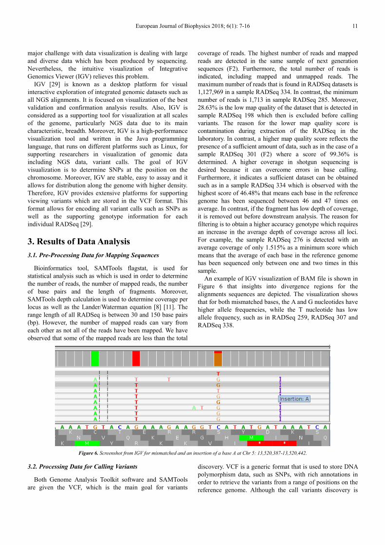
3.3.2. Results of Critical Values for Chi-Square Test

The certainty cutoff of critical value for Chi-Square test is

determined by 3.84. Reliable SNPs have a critical value of

Chi-square less than 3.84 and their distribution is shown in

Figure 9.


Figure 9. Density distribution for critical value of Chi-Square test for each

SNPs.

3.3.3. Results of P-Values

The four plots shown in all Figure 10, Figure 11, Figure 12

and Figure 13 show the distribution of all P-values calculated

for each SNP at loci. Reliable SNPs have P-value greater

than 0.05. In contrast, all SNPs that have P-values < 0.05 are

rejected (false positive). We noticed that only by Haplotype

Caller with joint genotypes algorithm have more reliable

SNPs, which have been detected.

Figure 10. P-values by first procedure.

Figure 11. P-values by second procedure.

Figure 12. P-values by third procedure.

Figure 13. P-values by fourth procedure.

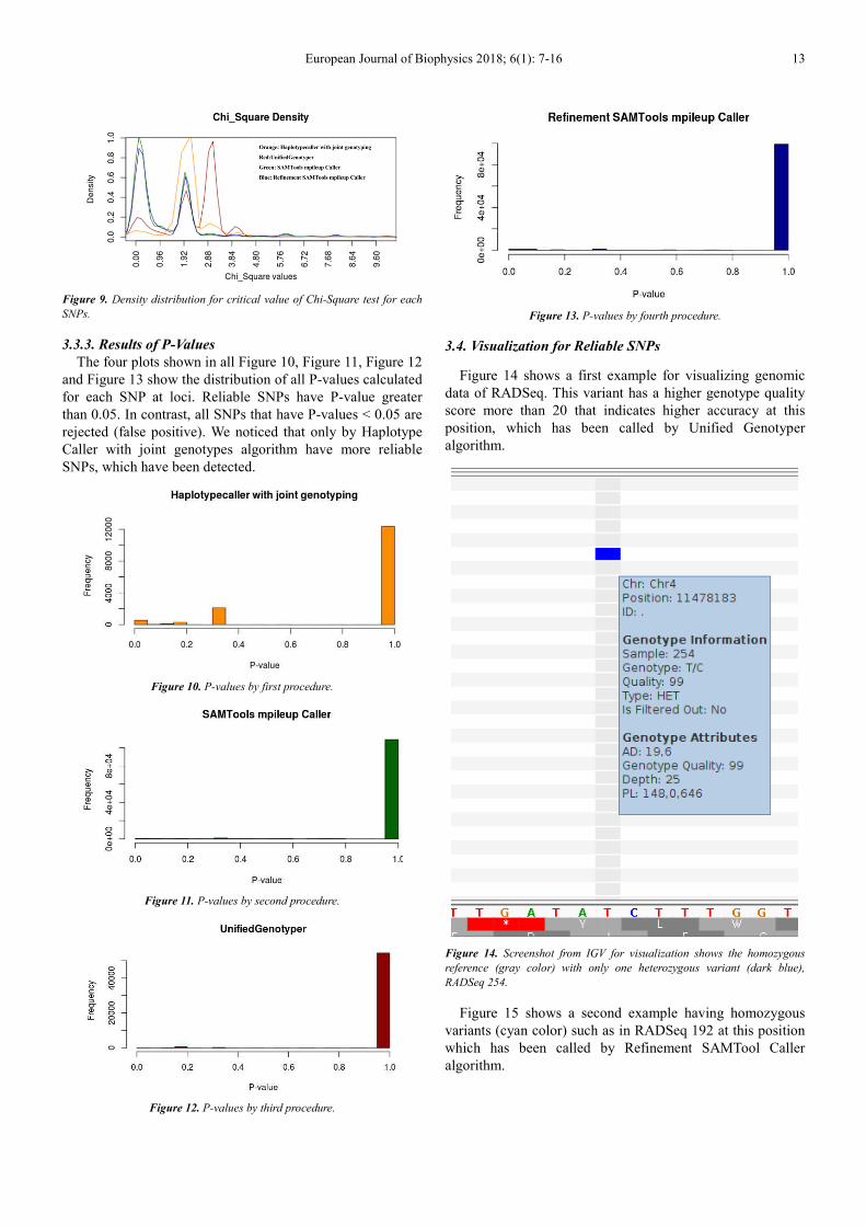
3.4. Visualization for Reliable SNPs

Figure 14 shows a first example for visualizing genomic

data of RADSeq. This variant has a higher genotype quality

score more than 20 that indicates higher accuracy at this

position, which has been called by Unified Genotyper

algorithm.

Figure 14. Screenshot from IGV for visualization shows the homozygous

reference (gray color) with only one heterozygous variant (dark blue),

RADSeq 254.

Figure 15 shows a second example having homozygous

variants (cyan color) such as in RADSeq 192 at this position

which has been called by Refinement SAMTool Caller

algorithm.


Figure 15. Screenshot from IGV for homozygous variants such as in

RADSeq 192 at this position.

The third example, Figure 16, of RADSeq 197 shows

homozygous reference (gray color) and homozygous variants

(cyan color) with heterozygous variants (dark blue) which

has a higher genotype quality score more than 60 and

indicates higher accuracy of (more than 99.9999%) that has

been called by Haplotype Caller algorithm.

Figure 16. Screenshot from IGV for visualization data in RADSeq 197.

Results of Chr C:

The fourth example is shown in Figure 17 of SNPs in

genetic material on the chromosome of chloroplast (Chr C).

These should all be 1/1 homozygous variants as mother`s

alleles such as the genetic variants at this position has been

called by Unified Genotyper procedure of Chr C.

Figure 17. Screenshot from IGV for homozygous variants for SNPs in

genetic material for Chr C.

4. Conclusions & Suggestions

The goal of this new genomic study was to identify high

density of markers across genomes using NGS techniques

such as RAD-Seq, particularly in organisms for which few

genomic resources presently exist. RAD-seq data was used to

identify SNPs and distinguish homozygous and heterozygous

variants in a population of Arabidopsis thaliana obtained by

crossbreeding two strains. To accomplish this, a customized

pipeline was used that included four different variant callers

which are based on the Genome Analysis Toolkit (GATK)

[30] and SAMTools/BCFTools [11] [15] [30]. Both GATK

and SAMTools produce genotype information in groups of

individuals. These tools are meant to operate on top of a

genome, for example by detecting nucleotide variants

through matches to the reference sequence.

Other previous pipeline is available to provide several

common output formats to integrate Stacks-generated

genotype data of RAD-Seq with downstream analysis

packages. In contrast, SAMTools/BCFTools and GATK can

call SNPs in multiple samples of RAD-Seq and then can

generate allele frequencies, but all populations are managed

by hand as merging all BAM files in order to obtain one VCF

file that consists of multiple samples, as compared to the

integrated way that this occurs in Stacks. Furthermore, Stacks

was developed to have at its core a catalogue that works as an

internal reference for each project regardless according to the

presence of a genome [6]. All of these tools, the analysis ends with lists of SNPs

(‘analysis ready variants’) that can be used in subsequent


analyses but with some difficulty for the following reasons.

First, some SNPs have been detected due to errors during

variant calling. We could divide the SNP calling errors into

three classes: 1) preparing the sample libraries at the wet lab,

2) machine errors when sequences are generated from the

libraries, 3) software and mapping artefacts when the reads

are aligned. Therefore, quality filtering of variant calls is an

essential step that has been applied in order to minimize false

positive. Therefore, in order to obtain high specificity, a

number of filters were applied to eliminate false positives.

Second, parameters/thresholds required for the filters needed

to be set comprehensively in dependence of the data obtained.

Third, the final step consisted of the visualization of the

variants using Integrative Genomics Viewer (IGV) is

required. In contrast, a Stacks analysis starts with raw

sequencing reads and then progress through all analysis steps

to generate allele and genotype calls, a number of core

population genetics statistics and formatted output files [6].

Finally, the results in this study were very consistent and

indicated new pipeline for variants calling using NGS data,

especially RAD-Seq is developed. Thus, the pipeline presents

a valuable tool for exploring homozygous and heterozygous

variants. We concluded that results from our study will

provide practical and comprehensive guidance to more

accurate and consistent variant identification. On this basis

further research might be conducted as in the following: 1) A

comprehensive study of those genotypes for variants that

have been detected and refined. As most SNPs are found

within protein coding regions, to characterize the function

impact of each SNP would be interesting. For example, if the

coded amino acid does not change the protein, it is called a

synonymous SNP (as the codon is a 'synonym' for the amino

acid), while if the coded amino acid causes a change in the

protein, it is called a non-synonymous SNP, 2) the

identification of genetic markers that have typically been

involved in marker discovery of SNPs using RAD-Seq could

be used in the future to associate with the phenotypes. That is

to study variants which are associated with a phenotype

could be comprehensively studied in the future.

Acknowledgements

We are grateful to Max Planck Institue for Plant Breeding

Reascher, Xiangchao Gan, PhD and Professor Dr Miltos

Tsiantis. Wellness for their offering this job with new topic

Master project: bioinformatics and comparative genomics Nr:

Summer-2017.

References

[1] Allen, R. S., Nakasugi, K., Doran, R. L., Millar, A. A., & Waterhouse, P. M. (2013). Facile mutant identification via a single parental backcross method and application of whole genome sequencing based mapping pipelines. Frontiers in plant science, 4.

[2] Almgren, P., BENDAHL, P., Bengtsson, H., Hössjer, O., & Perfekt, R. (2003). Statistics in genetics. Lecture notes, Lund.

[3] Andrews, K. R., Good, J. M., Miller, M. R., Luikart, G., & Hohenlohe, P. A. (2016). Harnessing the power of radseq for ecological and evolutionary genomics. Nature Reviews Genetics, 17 (2), 81–92.

[4] Baird, N. A., Etter, P. D., Atwood, T. S., Currey, M. C., Shiver, A. L., Lewis, Z. A.,. Johnson, E. A. (2008). Rapid snp discovery and genetic mapping using sequenced rad markers. PloS one, 3 (10), e3376.

[5] Bergelson, J., Kreitman, M., & Nordborg, M. (n. d.). Columbia col-0: n28167 or cs28167 [Computer software manual]. Retrieved from https://www.arabidopsis.org/abrc/catalog/natural a ccession 5 html.

[6] Catchen, J., Hohenlohe, P. A., Amores, S. B. A., & Cresko, W. A. (2014 Nov 25). Stacks: An analysis tool set for population genomics. NIH Public Access, PMC.

[7] Danecek, P., Auton, A., Abecasis, G., Albers, C. A., Banks, E., DePristo, M. A.,... others (2011). The variant call format and vcftools. Bioinformatics, 27 (15), 2156–2158.

[8] Davey, J., & Blaxter, M. L. (2011). Radseq: next-generation population genetics. Briefingsin Functional Genomics, 9, 108.

[9] De Pristo, M. A., Banks, E., Poplin, R., Garimella, K. V., Maguire, J. R., Hartl, C.,... others (2011). A framework for variation discovery and genotyping using next-generation dna sequencing data. Nature genetics, 43 (5), 491–498.

[10] De Summa, S., Malerba, G., Pinto, R., Mori, A., Mijatovic, V., & Tommasi, S. (2017). Gatk hard filtering: tunable parameters to improve variant calling for next generation sequencing targeted gene panel data. BMC bioinformatics, 18 (5), 119.

[11] Emigh, T. H. (1980). A comparison of tests for hardy-weinberg equilibrium. Biometrics, 627–642. Group, S. F. S. W., et al. (2014). Sequence alignment/map format specification. Tech. rep. Version 1. 2015. url: http://samtools. github. io/hts-specs/SAMv1. pdf (visited on 01/04/2015).

[12] Herzeel, C., Costanza, P., Ashby, T., & Wuyts, R. (2013). Performance analysis of bwa alignment (Tech. Rep.). Technical Report Exascience Life Lab. 59.

[13] Ishii, K., Kazama, Y., Hirano, T., Hamada, M., Ono, Y., Yamada, M., & Abe, T. (2016). Amap: A pipeline for whole-genome mutation detection in arabidopsis thaliana. Genes & genetic systems, 91 (4), 229–233.

[14] Kosugi, S., Natsume, S., Yoshida, K., MacLean, D., Cano, L., Kamoun, S., & Terauchi, R. (2013). Coval: Improving alignment quality and variant calling accuracy for next-generation sequencing data. PLoS one.

[15] Li, H. (2010). Mathematical notes on samtools algorithms. October.

[16] Li, H. (2013). Aligning sequence reads, clone sequences and assembly contigs with bwa-mem. arXiv preprint arXiv.

[17] Li, H. (2014). Toward better understanding of artifacts in variant calling from high-coverage samples. Bioinformatics, 30 (20), 2843–2851.

[18] Li, H., & Durbin, R. (2010). Fast and accurate long-read alignment with burrows–wheeler-transform. Bioinformatics, 26 (5), 589–595.


[19] Li, H., Handsaker, B., Wysoker, A., Fennell, T., Ruan, J., Homer, N.,... Durbin, R. (2009). The sequence alignment/map format and samtools. Bioinformatics, 25 (16), 2078–2079.

[20] Marrano, A., Birolo, G., Prazzoli, M. L., Lorenzi, S., Valle, G., & Grando, M. S. (2017). Snp-discovery by rad-sequencing in a germplasm collection of wild and cultivated grapevines (v. vinifera l.). PloS one, 12 (1), e0170655.

[21] McCormick, R. F., Truong, S. K., & Mullet, J. E. (2015). Rig: recalibration and interrelation of genomic sequence data with the gatk. G3: Genes, Genomes, Genetics, 5 (4), 655–665.

[22] McKenna, A., et al. (2016). The genome analysis toolkit: A mapreduce framework for analyzing next-generation dna sequencing data. genomet+ research. published in advance jul. 19, 2010.

[23] Molnar, M., & Ilie, L. (2015). Correcting illumina data. Briefings in bioinformatics, 16, 588–599.

[24] Nielsen, R., Paul, J. S., Albrechtsen, A., & Song, Y. S. (2011). Genotype and snp calling from next-generation sequencing data. Nature Reviews Genetics, 12 (6), 443–451.

[25] Ossowski, S., Schneeberger, K., Clark, R. M., Lanz, C., Warthmann, N., & Weigel, D. (2008). Sequencing of natural strains of arabidopsis thaliana with short reads. Genome research, 18 (12), 2024–2033.

[26] Peter J. A. Cock, Christopher J Fields, Naohisa Goto, Michael Lheuer, Peter M Rice. The Sanger FASTQ file format for sequences with quality scores, and the Solexa/Illumina

FASTQ variants. Nucleic Acids Research, Vol (38), No (6). 16 December 2009.

[27] Runs, E. S. (n. d.). Estimating sequencing coverage.

[28] Thorvaldsdóttir, H., Robinson, J. T., & Mesirov, J. P. (2013). Integrative genomics viewer (igv): high-performance genomics data visualization and exploration. Briefings in bioinformatics.

[29] Van der Auwera, G. A., Carneiro, M. O., Hartl, C., Poplin, R., del Angel, G., Levy Moonshine, A.,... others (2013). From fastq data to high-confidence variant 60 calls: the genome analysis toolkit best practices pipeline. Current protocols in bioinformatics, 11–10.

[30] Wang, J., Scofield, D., Street, N. R., & Ingvarsson, P. K. (2015). Variant calling using ngs data in european aspen (populus tremula). In Advances in the understanding of biological sciences using next generation sequencing (ngs) approaches (pp. 43–61). Springer.

[31] Warden, C. D., Adamson, A. W., Neuhausen, S. L., & Wu, X. (2014). Detailed comparison of two popular variant calling packages for exome and targeted exon studies. Peer J, 2, e600.

[32] Weigel, D., & Mott, R. (2009). The 1001 genomes project for arabidopsis thaliana. Genome biology, 10 (5), 107.

[33] Wigginton, J. E., Cutler, D. J., & Abecasis, G. R. (2005). A note on exact tests of hardy-weinberg equilibrium. The American Journal of Human Genetics, 76 (5), 887–893.

Documents

A Pipeline for Markers Selection Using Restriction Site