A pedagogic review on designing model topological insulators

Tanmoy Das Department of Physics, Indian Institute of Science, Bangalore- 560012, India.

Following the centuries old concept of the quantization of flux through a Gaussian curvature (Euler characteristic)

and its successive dispersal into various condensed matter properties such as quantum Hall effect, and topological

invariants, we can establish a simple and fairly universal understanding of various modern topological insulators

(TIs). Formation of a periodic lattice (which is a non-trivial Gaussian curvature) of ‘cyclotron orbits’ with applied

magnetic field, or ‘chiral orbits’ with fictitious ‘momentum space magnetic field’ (Berry curvature) guarantees its

flux quantization, and thus integer quantum Hall (IQH), and quantum spin-Hall (QSH) insulators, respectively,

occur. The bulk-boundary correspondence associated with all classes of TIs dictates that some sort of pumping or

polarization of a ‘quantity’ at the boundary must be associated with the flux quantization or topological invariant

in the bulk. Unlike charge or spin polarizations at the edge for IQH and QSH states, the time-reversal (TR)

invariant Z2 TIs pump a mathematical quantity called ‘TR polarization’ to the surface. This requires that the

valence electron’s wavefunction (say, 𝜓↑(𝐤)) switches to its TR conjugate (𝜓↓∗(−𝐤)) odd number of times in half

of the Brillouin zone. These two universal features can be considered as ‘targets’ to design and predict various

TIs. For example, we demonstrate that when two adjacent atomic chains or layers are assembled with opposite

spin-orbit coupling (SOC), serving as the TR partner to each other, the system naturally becomes a Z2 TI. This

review delivers a holistic overview on various concepts, computational schemes, and engineering principles of

TIs.

CONTENTS

I. Introduction

II. Theories of topological invariants

A. Gaussian curvature, Euler number and genus

B. Laughlin’s argument and TKNN invariant

C. QH calculation in arbitrary parameter space

D. Berry connection, and Berry curvature

E. Chern number without magnetic field

1. Spin Chern number

2. Mirror Chern number

F. Z2 invariant and time-reversal polarization

G. Z2 calculation with inversion symmetry

H. Z2 calculation without inversion symmetry

I. Axion angle as topological invariant

J. Topological invariant for interacting systems

K. Topological invariant for superconductors

L. Adiabatic continuity

M. Bulk-boundary correspondence

III. Engineering TIs

A. Engineering topological ‘chiral orbits’ in 2D

B. Engineering 3D TIs with Rashba-bilayers

C. Spatial modulation of ‘chiral orbits’ and

quantum spin-Hall density wave insulator

D. Spinless orbital texture inversion induced

topological ‘chiral orbits’

IV. Conclusions and outlook

Email: tnmydas@gmail.com

I. Introduction

Phase transition is distinguished by a change in

symmetry, involving either a reduction or addition of

symmetry in the ground state. A reduction of

symmetry, which commonly involves translational,

time-reversal (TR), rotational, gauge symmetries,

among others, leads to a classical/quantum phase

transition, and is defined by an order parameter within

the Landau's paradigm. On the contrary a topological

phase is defined by the emergence of a new quantum

number (such as Chern number, Z2 invariant), arising

from the geometry or topology of the band structure.

The topological invariant can be understood from a

pure mathematical formalism of the Euler

characteristic or Euler number. This implies that the

net flux through a Gaussian curvature is always

quantized. This is precisely what happens, according

to Laughlin’s argument,1 in two-dimensional (2D)

lattices (which can be represented by a torus - a

Gaussian curvature) when magnetic field is applied

perpendicular to it. In this case, the magnetic flux

through the 2D system or torus remains quantized,

giving rise to integer quantum Hall (IQH) effect. This

is the first realization of topological invariant in

condensed matter science.

2

IQH is a well understood phenomenon, with different

ways to quantify its topological invariants. For

example, Thouless, Kohmoto, Nightingale, and Nijs

(TKNN) have shown that the IQH effect can also be

understood from the Berry phase paradigm in the

momentum space.2 The corresponding topological

invariant is thus known as TKNN number or Chern

number. Haldane proposed a pioneering idea to obtain

quantum Hall (QH) effect without external magnetic

field in a honeycomb lattice.3 Honeycomb lattice has

two different sublattices. With the application of an

external gauge field, the intra-sublattice hoppings

possess chiral motion, and the chirality of two

sublattices becomes opposite to each other. Different

intra-sublattice electron hopping commence counter-

propagating triangular ‘cyclotron orbits’, each

threading opposite ‘magnetic fields’. As we will go

along in this review, we will identify that the

formation of localized ‘cyclotron orbitals’ in 2D lattice

without a magnetic field, which we call “chiral orbits”,

is a key ingredient to obtain QH effect. Each such

“chiral orbit” now encloses integer flux quanta, in the

same language of the IQH effect, and due to TR

symmetry breaking a net QH effect survives.

The next development to the TI field was put forward

by Kane and Mele in 2005 for obtaining TR invariant

TIs, as known by Z2 TI.4 They realized that Haldane’s

‘gauge field’ can be achieved by spin-orbit coupling

(SOC). Owing to the spin-momentum locking, the

right- and left-moving electrons have opposite spin

polarizations. Since the TR symmetry is intact here,

the flux passing through different spin-resolved ‘chiral

orbits’ in a 2D lattice are exactly equal but opposite.

This makes the net flux to be zero, leading to no

charge pumping to the edge, but the difference

between the two fluxes is finite, giving rise to a net

spin-resolved QH effect, as known by quantum spin-

Hall (QSH) effect. This is the foundation of the 2D Z2

TI.

The generalization of the Z2 topological invariant to

3D cannot, however, be easily done in terms of ‘chiral

orbit’ formations, except in special cases of layered

systems and heterostructures.5 There are several

mathematical formulations of the Z2 invariant4,6–14.

Among which, the Kane-Mele method of TR

polarization is widely used.4 They proposed a

derivation of the bulk Z2 topological invariant from the

bulk-boundary correspondence which is a necessary

condition for all topological invariants. Recall that in

the case of IQH and QSH insulators, charge and spin

are accumulated at the edge. Based on this, they

enquired that something similar must be pumped to the

boundary in Z2 TIs. Since QSH insulator also belongs

to the Z2 class, the quantity that is pumped to the edge

must accommodate spin as a subset. Since the spin-up

state at the +k and spin-down state at –k are TR

conjugates to each other, Kane-Mele proposed that a

more general mathematical quantity, called ‘TR

polarization’, is accumulated at the edge in this case.

Here electrons possessing a particular wavefunction

and their TR conjugate partners move to different

edges. This incipiently requires that the electron

exchanges it TR partner odd number of times in

traversing half-of the Brillouin zone (BZ). In what

follows, Z2 topological invariant is nothing but counts

of the number TR partner exchanges; odd number

corresponds to Z2 invariant 𝜈 = 1, while even number

implies 𝜈 = 0. Since the TR symmetric topological

invariant only takes two values, it has Z2 symmetry.

But TR breaking IQH state can take arbitrarily large

Chern number.

Chirality of electrons is an essential ingredient for TIs,

which is obtained either by magnetic field, or in

bipartite lattice (such as staggered hopping in Su-

Schrieffer-Heeger (SSH) lattice,15 or graphene) or via

SOC. Such chirality can also arise from the orbital

texture inversion between even and odd parity orbitals

at the TR invariant points, leading to a distinct class of

spinless topological and Dirac materials.16,17 In simple

term, chirality means that the electron’s hopping in

lattice must be complex. As the electron’s hopping

encloses a ‘chiral orbit’, the complex phase manifests

into a magnetic field at the center – either applied, or

self-generated (Berry curvature). For Z2 class, the TR

partner switching, discussed in the previous paragraph,

is nothing but the exchange of electron’s phase to its

complex conjugate odd number of times in half-of the

BZ.

Subsequently, Fu-Kane simplified the calculation of Z2

invariant by using the parity analysis.7 They showed

that if a system has both TR and inversion symmetries,

the Z2 topological invariant can be computed simply

by counting how many times the electron exchanges it

parity at the TR invariant momenta. If the valence

band is not fully defined by a single parity, rather it

exchanges parities odd number of times with the

3

conduction band (as in the case of TR partner

exchange), it gives a non-trivial topological invariant.

This is also equivalent to chirality inversion in special

cases as we will demonstrate in our engineering

procedures. The band gap between the opposite parity

conduction and valence bands at the TR invariant

momenta also serves as the ‘negative’ Dirac mass in

the Dirac equation.9,18 The consequence of this band

inversion is very rich, allowing protected gapless

surface or edge states with Dirac cone. This provides

an alternative springboard to obtain numerous exotic

properties originally proposed by solving Dirac

equation in the high-energy theories.

This simple theory leads to the search of materials

with band inversions at the TR invariant k-points as a

simple tool to identify Z2 TI. The mechanism of parity

inversion is not unique, and can in-principle vary to a

wide range of tuning parameters as well as electron-

electron interactions. Among them, SOC is responsible

for the band inversion in most of the known TIs.

Initially, the search for TI had been very much ‘blind-

folded’, seeking materials with odd number of band

inversions triggered by SOC.6,9,18,19 Subsequently,

more advanced methods of TI materials genome such

as ‘adiabatic transformation’ method was developed,20

which can be applied to systems without inversion

symmetry. In this method, one starts with a known TI,

and continuously tunes the atomic number of the

constituent elements, and arrives at a new material. In

this process if the band gap does not close and reopen

at the TR invariant points, the new material must also

be a non-trivial TI. These two methods have enabled

the discoveries of a rich variety of TI materials.

Subsequently, various distinct classes of TI are

predicted and discovered. For example, mirror

symmetry and p-wave superconducting pairing

symmetry can lead to two distinct classes of TIs,

called topological crystalline insulator,21 and

topological superconductor,22,23 respectively.

Spontaneous TR symmetry breaking TIs, without

magnetic field, are known as quantum anomalous Hall

(QAH) insulator in 2D, or topological axion insulator

in 3D.24,25 The axion insulator has a quantized

magnetoelectric response identical to that of a (strong)

TI, but lacks the protected surface states of the TI.

Other methods of obtaining insulating state such as

disorder, Kondo effect, or Hubbard interaction,

associated with odd number of band inversions, are

also proposed to give topological Anderson

insulator,26,27 topological Kondo insulator,28 and

topological Mott insulator29, respectively. Finally, a

new class of TI is proposed by the present author,

which is called quantum spin-Hall density wave

(QSHDW) insulator in quasi-2D.30

When two opposite

chiral states are significantly nested in a given system,

it renders a transitional symmetry breaking Landau

order parameter (forming spin-orbit density wave31,32),

which can be associated with odd number of band

inversions and Z2 topological invariant for a special

nesting vector. In this case, the parity or chirality

inversion occurs in the real space between different

lattice sites, breaking the transitional symmetry, but

not the TR symmetry.

Density functional theory (DFT) 18,19 calculations take

a preceding role in predicting most of the TIs, many of

which are followed by experimental realizations.

Owing to weak SOC in graphene, this material has not

been realized to be intrinsic TI despite its first

prediction. HgTe/CdTe quantum well state were

predicted to be 2D TI,9 which was followed by its

experimental realization.33 The 3D topological

semimetal predicted,8 and realized34 is Bi1-xSbx. The

first 3D TI was discovered in Bi2Se3, Bi2Te3, Sb2Te3,

family both theoretically and experimentally.18,19,35

This is followed by a series of predictions of 3D TIs

including gray tin,7 HgTe, InAs,20 ternary tetramytes

GemBi2nTe(m+3n) series,36 half-Huesler compounds,37,38

Tl-based III-V-VI2 chalcogenides,39,40 ternary I-III-

VI2 and II-IV-V2 chalcopyrites, I3–V–VI4

famatinites, and quaternary I2–II–IV–VI4

chalcogenides,41 Li2AgSb,20 LiAuSe honeycomb

lattice,42 β-Ag2Te,43 non-centrosymmetric BiTeX

(X=Cl, I, Br)44–46. Recently a number of materials are

discovered to have stable 2D structure, among which

Si, Ge46, Sn,47 As,48 Bi,49,50 P51 are predicted to exhibit

QSH insulating state with SOC, and with other tuning.

Pb1-xSnxSe/Te52–54 and SnS55 are the only topological

crystalline insulators known to date. f-electron based

compounds such as SmB6,28,56 YbB6,

57 are predicted to

be topological Kondo insulators, while PuB6 is

considered a topological Mott insulator.58 URu2Si2 is

considered as a candidate material for the spin-orbit

density wave induced hidden topological order

system.31,59,60 Ir, and Os-based oxides are proposed to

be axion insulators.25 The list of QAH insulator is

rather small,61 most of which require external tuning

4

with magnetic doping and thin films. LaX (X = Br, I

and Cl) family is predicted to be intrinsic QAH

insulator with sizable band gap for applications.62 A

complete materials repository and their individual

properties can be found in Refs. 63,64.

Despite this tremendous success as well as continuing

research activities for harvesting more TI materials,

the real struggle with the presently available materials

is that the unwanted bulk conduction band lies below

the Fermi level, and contributes to the transport

phenomena. There have been considerable efforts to

eliminate the bulk band above the Fermi level by

chemical doping,65,66 pressure,67,68 photo-doping,69

heterostructure,70,71 etc. All these efforts have however

little success and the ultimate aim for obtaining pure

edge current remained unachieved. In the 2D

counterpart, the challenge extends to the lack of

material diversity. Moreover, although HgTe/CdTe33

and InAs/GaSb72 are demonstrated by transport

measurement to show QSH behavior, but for other

measurements, these samples are not very useful.

A jump-start to the field was offered by various

engineering principles for TIs. There have also been

considerable efforts to engineer TIs by proximity

induced SOC in graphene through adatoms,73 or with

interfacing with transition metal di-chalcogenides74,75,

and in artificial heterostructures,5,16,76 and in optical

lattices.77–79 Artificially grown heterostructures can be

very versatile as they offer higher materials flexibility

and tunability. The present author has proposed a

number of design principles for engineering quasi-

1D,30 2D,79 as well as 3D TI5,16 by decorating atoms or

layers. The basic idea lies in generating ‘chiral orbits’

in a periodic fashion without breaking TR symmetry in

2D plane. Each ‘chiral orbit’ thereby encloses a

pseudo-magnetic field (Berry curvature) in the same

sense as in the TKNN language and commence

quantized Chern number.79 In real-space, electron-

electron interaction induced translational symmetry

breaking can lead to chirality inversion between

different sublattices, leading to a new type of Z2

quantum order which is associated with topological

invariant and edge states.30 The 3D generalization

follows similarly in that the adjacent layers should

have opposite SOC, such that they serve as TR partner

to each other. As the quantum tunneling between them

drives a band inversion, a 3D TI naturally arises.5 A

heterostructure of even and odd orbital orbitals is also

a fertile setup to generate Dirac materials.16 The

second part of this article discusses various forms of

these engineering principles.

TI has been reviewed extensively in various forms.

Three review articles are published in the Review of

Modern Physics.23,63,80 Topological band theory63,81

and topological field theories14 are also discussed

extensively. A materials repository can be found in

Refs.63,64 Topological superconductors are reviewed in

Refs. 23,82,83. QSH84 and QAH61 insulators are also

reviewed separately. Reviews of Dirac and Weyl

materials can be found in Refs. 85,86. Few books are

available to understand the basics of various TIs .87,88

II. Theories of topological invariants Topological band theory encompasses broadly defined

computational schemes for the calculations of various

topological invariants in systems with or without TR

symmetry, inversion symmetry, particle-hole

symmetry, and mirror symmetry. Depending on larger

number of symmetries present in the Hamiltonian, the

computation of the corresponding topological invariant

simplifies accordingly. Both Chern number and Z2

invariants are defined by single particle wavefunction,

and can be calculated using the tight-binding or

Wannier wavefunction within the DFT. For weakly

interacting systems, such calculation can be extended

to the quasipaprticle spectrum within a Fermi-liquid or

mean-field theory. For strongly correlated systems, the

Chern number can be calculated by using the self-

energy dressed Green’s function.89,90 In addition to

rigorous calculations of Chern number or Z2

invariants, there are also other simplified methods

which can be used for preliminary diagnosis of a

potential TI. For examples, one can determine the non-

trivial TI by simply counting the odd number of band

inversions at the TR symmetric k-points, or employing

the adiabatic (band gap-) continuity between a known

TI and an unknown insulator, and/or bulk-boundary

correspondence.

We start this section with the historical development

of topology which forms the basis for modern

topological invariant. Then we discuss various

topological invariant calculations based on the number

of symmetries present in a given case. Across most of

the methods we discussed below, some unified

concepts can be excavated which combine diverse

formalisms of topological invariant. Among them, we

5

have: (i) Complex

phase associated

with electron

hopping with

quantized phase

winding; (ii)

Formation of

cyclotron or

‘chiral orbits’ in

periodic lattice

(Gaussian

curvature); (iii)

Odd number of

exchange of

electron’s complex

phase, or chirality

or TR conjugate in

half of the BZ; (iv) Search for bulk property (s) which

can lead to accumulation of charge (IQH), or spin,

(QSH), or TR polarizibility (Z2 class). We will discuss

below such corresponding basic principles used for the

derivation of various topological invariants.

A. Gaussian curvature, Euler number, and genus

The inception of the concept of invariants can be

traced back to the times of Leonhard Euler and Carl

Friedrich Gauss in the 18th century. Gaussian curvature

can be a good starting point to build up the discussion.

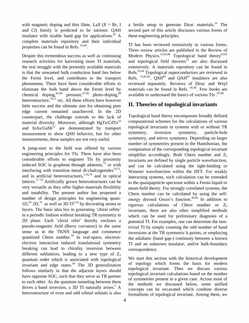
It is defined by the product of two principle curvatures

(𝜅1, 𝜅2), along any two perpendicular directions at a

given point (see Fig. 1) as 𝛫 = 𝜅1𝜅2. If a principle

curvature has a minimum (maximum) at the point

(convex and concave curvatures), we assign its value

to be -1 (+1). In this sense, if a point on the surface has

minima or maxima in both principle directions, then

the corresponding Gaussian curvature is +1 [Figs 1(c-

d)]. The outer and inner surfaces of a sphere provide

the corresponding examples, both being topologically

equivalent. On the other hand, if a point

simultaneously possess maximum and minimum in the

two principle directions, the Gaussian curvature yields

-1 [Fig. 1(e)]. The camel’s back or a torus is non-

trivial Gaussian curvature with Κ = -1.

Euler characteristic (also known as Euler number)

dictates that the flux through a Gaussian curvature is

always quantized as

∯ 𝛫𝑑𝑆

𝑆= 2𝜋𝜈, where ν = integer. (1)

The above integral formula can also be expressed in

terms of the Gauss-Bonnett formula, giving a

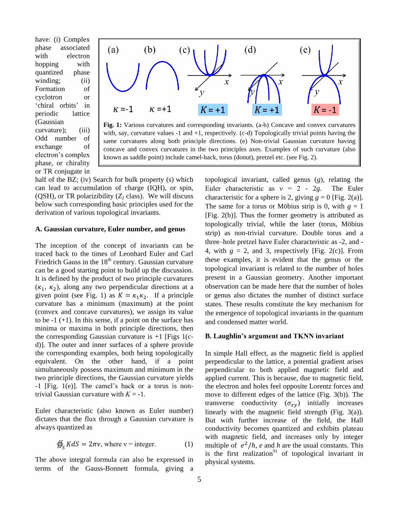
topological invariant, called genus (g), relating the

Euler characteristic as ν = 2 - 2g. The Euler

characteristic for a sphere is 2, giving g = 0 [Fig. 2(a)].

The same for a torus or Möbius strip is 0, with g = 1

[Fig. 2(b)]. Thus the former geometry is attributed as

topologically trivial, while the later (torus, Möbius

strip) as non-trivial curvature. Double torus and a

three–hole pretzel have Euler characteristic as -2, and -

4, with g = 2, and 3, respectively [Fig. 2(c)]. From

these examples, it is evident that the genus or the

topological invariant is related to the number of holes

present in a Gaussian geometry. Another important

observation can be made here that the number of holes

or genus also dictates the number of distinct surface

states. These results constitute the key mechanism for

the emergence of topological invariants in the quantum

and condensed matter world.

B. Laughlin’s argument and TKNN invariant

In simple Hall effect, as the magnetic field is applied

perpendicular to the lattice, a potential gradient arises

perpendicular to both applied magnetic field and

applied current. This is because, due to magnetic field,

the electron and holes feel opposite Lorentz forces and

move to different edges of the lattice (Fig. 3(b)). The

transverse conductivity (𝜎𝑥𝑦) initially increases

linearly with the magnetic field strength (Fig. 3(a)).

But with further increase of the field, the Hall

conductivity becomes quantized and exhibits plateau

with magnetic field, and increases only by integer

multiple of 𝑒2/ℎ, e and h are the usual constants. This

is the first realization91 of topological invariant in

physical systems.

Fig. 1: Various curvatures and corresponding invariants. (a-b) Concave and convex curvatures

with, say, curvature values -1 and +1, respectively. (c-d) Topologically trivial points having the

same curvatures along both principle directions. (e) Non-trivial Gaussian curvature having

concave and convex curvatures in the two principles axes. Examples of such curvature (also

known as saddle point) include camel-back, torus (donut), pretzel etc. (see Fig. 2).

6

In the QH regime, electrons form cyclotron orbits in

the bulk and becomes localized (see Fig. 3(c)).

Although magnetic field breaks translation asymmetry,

but as the magnetic field is sufficiently large, the

radius of the cyclotron orbits reduces. Here the

cyclotron orbits form a larger magnetic unit cell,

whose cross-sectional area changes with the field

strength. R.B. Laughlin1 recognized that the periodic

lattice in a 2D plane can be represented by a torus,

forming a non-trivial Gaussian curvature [Fig. 2(b)].

The magnetic flux through the magnetic torus is thus

quantized, according to the Euler integral in Eq. (1), as

φ = ∯ 𝐵𝑧𝑑𝑆

𝑆∈MT= 𝐵𝑧𝑆 = 𝜈 ℎ/𝑒, (2)

where 𝐵𝑧 is the perpendicular component of the

applied magnetic field, S is the cross-sectional area of

the magnetic torus (MT), ν is integer. So the question

is as the magnetic field is continuously increased, how

the area of the magnetic unit cell changes to respect

the above quantization condition and how the bulk

topology arises?

Thouless, Kohmoto, Nightingale, and Nijs (TKNN)2

argued that the area of the magnetic unit cell increases

as integer multiple of the original unit cell (𝑆0 = 𝑎𝑏)

as, 𝑆 = 𝑞𝑆0, where a and b are the lattice parameters

and q is an integer. Therefore the flux through the

original unit cell is a rational number times the flux

quanta (φ0 = ℎ 𝑒⁄ .): φ = 𝐵(𝑎𝑏) =𝜈

𝑞𝜑0. Once a

magnetic unit cell is defined, we can now Fourier

transform to the corresponding momentum space by

redefining a magnetic translational symmetry and

quantify a bulk topological invariant. We recall that

here the Hall conductivity is itself a topological

invariant: 𝜎𝑥𝑦 = 𝑣𝑒2/ℎ, where 𝑣 is called TKNN or

Chern number. Hall conductivity can be calculated

from the Kubo formula using current-current

correlation function. Therefore, from the general Kubo

formula for conductivity, we can obtain our first

definition of a topological invariant or the Chern

number for the nth band (𝜈𝑛) as

𝜈𝑛 = 𝑖 ∑

𝐤,𝑛′≠𝑛

(𝑓(𝐸𝑛𝐤) − 𝑓(𝐸𝑛′𝐤))

×

[⟨𝜓𝑛(𝐤)|𝜕𝐻𝜕𝑘𝑥

|𝜓𝑛′(𝐤)⟩ ⟨𝜓𝑛′(𝐤)|𝜕𝐻𝜕𝑘𝑦

|𝜓𝑛(𝐤)⟩]

(𝐸𝑛𝐤 − 𝐸𝑛′𝐤)2 (3)

where 𝐸𝑛𝑘 is the eigenvalue of the Hamiltonian H and

𝜓𝑛(𝑘) is the Wannier wavefunction, and 𝑓(𝐸𝑛𝑘) is the

Fermi-Dirac distribution function.

C. Quantum Hall calculation in arbitrary

parameter space

The above formula is based on the variation of the

Hamiltonian in two orthogonal momentum directions

and thus implicitly assumes a periodicity of the lattice.

In some cases, as in disordered lattice, where a proper

unit cell is difficult to define, the above formula

apparently fails. However, Niu, Thouless and Wu92

generalized their TKNN invariant calculations to any

Fig. 2: Various Gaussian curvatures. (a) A sphere having convex curvatures in both directions represents a

topologically trivial geometry. (b) A sphere with a hole gives a non-trivial topology with a single surface. In the

language of topology, shape does not matter as long as they have the same geometry. For this reason, orange with a

hole or full shape donut or distorted donut or even a coffee cup represent the same topology (g = 1) with one hole. (c)

For the same reason, a pretzel is topologically distinct from the former two classes, having three holes or three

topologically distinct surfaces. A 2D periodic lattice can be represented by a torus as shown in (b), in which magnetic

field is applied perpendicular to both x- and y-directions.

7

two arbitrary parameter space, by implementing the

so-called “twisted boundary condition”. They

introduced two fictitious parameters α, β (which does

not require to have any physical relevance) and

demanded that the lattice is periodic under them as

𝜓(𝑥𝑖 + 𝐿1) = 𝑒𝑖𝛼𝐿1𝑒𝑖(𝑒𝐵 ℏ⁄ )𝑦𝑖𝐿1𝜓(𝑥𝑖),

𝜓(𝑦𝑖 + 𝐿2) = 𝑒𝑖𝛽𝐿2𝜓(𝑦𝑖). (4)

Here 𝑥𝑖 , 𝑦𝑖 are the lattice site indices, and 𝐿1, 𝐿2

represent the system size. In this case, the velocity

operators can be rewritten as 𝑣𝑥 =𝜕𝐻

𝜕𝑘𝑥→

𝜕𝐻

𝜕𝛼, and

𝑣𝑦 =𝜕𝐻

𝜕𝑘𝑦→

𝜕𝐻

𝜕𝛽, and the QH invariant can be

calculated in the (𝛼, 𝛽) space by using Eq. (3). This

generalization unravels an important insight that as the

Hamiltonian is adiabatically varied in any closed

parameter space, it gives the same topological

invariant. This implies that as the particle returns to its

starting points, the expectation value of the velocity

operators remains the same, but its wavefunction itself

acquires an additional phase. This phase turns out be

the Berry phase, proposed independently.93 The

expectation value of the velocity operator in any

parameter space is an important factor for topological

invariant, with the only requirement for a given

parameter space is that it has to be periodic (Gaussian

curvature), but not necessarily a physical parameter.

This is crucial for the conceptualization of the ‘chiral

orbit’ we use for the QSH effect which implies that

‘chiral orbit’ can be a mathematical object which can

be ‘created’ in any periodic parameter space for the

calculation of the topological invariant in 2D systems.

For the same reason, when a system is driven

periodically with time, the corresponding time

evolution of the Hamiltonian (Floquet Hamiltonian)

can also give rise to a ‘Berry phase’ in the time-

domain and lead to QH or topological phase.

D. Berry connection and curvature

The above section discussed how an applied magnetic

field’s flux quantization leads to the IQH as computed

within the Kubo formula. Now we can reverse our

derivation, and start with the Kubo formula version of

the topological invariant in Eq. (3), and define a band

dependent ‘magnetic field’ in the momentum space

𝐅𝑛(𝐤). We again demand that its flux in the reciprocal

space is quantized:

𝜈𝑛 =1

ΩBZ∬ 𝐅𝒏(𝐤)

BZ∙ 𝐧 𝑑2𝑘 = ∮ 𝐀(𝐤) ∙ 𝑑𝐤

𝜕𝐵𝑍, (5)

where ΩBZ is the BZ phase space area. In the last step,

we have employed the Stokes’ theorem, which

allowed us to define a momentum space ‘vector

potential’ as 𝐅𝒏(𝐤) = 𝛁𝑘 × 𝑨𝒏(𝐤). The formalism for

F(k) is simply the right-hand side of Eq. (3), and that

for A(k) can also be obtained subsequently. Another

elegant formalism for F and A can be obtained by

using the identity

|𝜕𝑘𝑖𝜓𝑛(𝐤)⟩ = ∑

⟨𝜓𝑛′(𝐤)|𝜕𝐻𝜕𝑘𝑖

|𝜓𝑛(𝐤)⟩

𝐸𝑛𝐤 − 𝐸𝑛′𝐤 |𝜓𝑛′(𝐤)⟩,

𝑛′≠𝑛

(6)

which yields

8

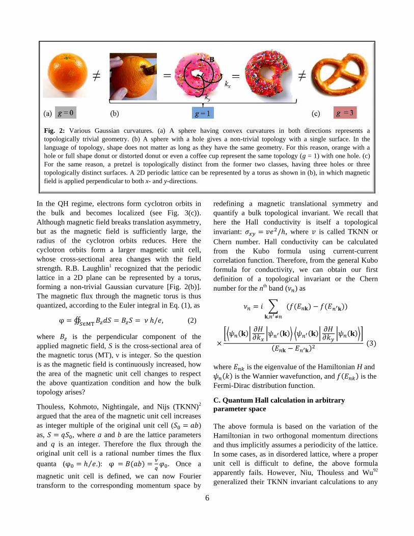
Fig. 4: Haldane model. The net inter-sublattice

hopping 𝑡1𝑒𝑖𝑘𝑎 remains complex, since its complex

conjugate partner 𝑡1𝑒−𝑖𝑘𝑎 is absent. On the other

hand, the net intra-sublattice hopping 𝑡2𝑒𝑖𝑘𝑏 +

𝑡2𝑒−𝑖𝑘𝑏 = 2 cos ( 𝑘𝑏) becomes real. Haldane added an

extrinsic phase (φ) into the hopping as 𝑡2𝑒𝑖(𝑘𝑏+𝜑), with

opposite phase for different sublattices (blue and red).

Therefore, the corresponding flux in the blue and red

triangles are equal but opposite.

𝐅𝒏(𝐤) = 𝑖⟨𝛁𝑘𝜓𝑛(𝐤)| × |𝛁𝑘𝜓𝑛(𝐤)⟩, (7)

𝐀𝒏(𝐤) = 𝑖⟨𝜓𝑛(𝐤)|𝛁𝑘𝜓𝑛(𝐤)⟩. (8)

To further elucidate the physical significance, we refer

back to Eq. (5) which can be can be compared with the

Peierls phase in real space, acquired by a charged

particle moving in a magnetic field, 𝜑 = ∫ 𝐀(𝐫) ∙ 𝑑𝐥𝑐2

𝑐1,

where A(r) is the vector potential, and c1 and c2 are

starting and end points of the path. This implies that

the topological invariant here is a momentum space

‘Peierls phase’ (equivalent to Aharonov-Bohm phase)

acquired by the electron in traversing a closed path in

the reciprocal space under an intrinsic gauge field

A(k). In this sense, 𝜈𝑛 is called the Berry phase,93 and

A(k) as the Berry connection, while F(k) is the Berry

curvature. Note that the Berry connection is gauge-

dependent and therefore topological invariant formulas

[such as axion angle formalism in Eq. (19) below]

involving it does not give an unambiguous result. On

the other hand, the Berry curvature is gauge invariant

and observable. Therefore, for a band which possess a

well-defined Berry phase in a close trajectory in the

momentum space (translational symmetry is assumed

as above), it possess an intrinsic Chern number, and

therefore can give rise to an IQH effect without the

application of an external magnetic field.

In the IQH effect, applied magnetic field provides the

‘chirality’ for the electrons to form cyclotron orbit.

Without magnetic field, the QH phenomena can be

thought of occurring in a reverse fashion. Here a self-

generated chirality of electrons creates a pseudo-

magnetic field (Berry curvature) in the process of

forming ‘chiral orbits’. In solid state systems, such

intrinsic chirality can stem from a multiple origins,

including SSH type staggered electron hopping,15

sublattice (as often referred to pseudospin) symmetry

in the hexagonal lattice,94 SOC,3 or certain type of

even-odd orbital texture mixing16,17. In a simpler term,

the chirality arises if the electron hopping is complex,

because it naturally accompanies a phase associated

with electron’s hopping. As the k-space magnetic field

or the Berry curvature threads through a periodic

lattice (Gaussian curvature), the Euler characteristic

ensures a quantization of the flux [Eq. (1)], and bulk

topological invariant arises. The intrinsic formation of

‘chiral orbit’ in a periodic lattice is the foundation of

TR invariant TIs, which however have different

interpretations and mathematical expositions such as

‘Pfaffian nodes’, ‘chiral vortex’, momentum-space

monopoles etc. as we will uncover below.

E. Chern number without magnetic field

If an 1D chain is made of two inequivalent sublattices,

the hopping between the two sublattices becomes

complex as used in the SSH model15 According to the

above prescription, the emergent ‘chiral’ hopping can

be associated with a winding number. Recall that in a

QH state, since the cyclotron orbits cannot complete a

full circle at the edges, it leads to the edge current, and

thus Hall effect arises. Something similar happens in

1D chain with chiral state. Since a localized chiral

orbit cannot be assumed in 1D, the chirality of the

electrons can be thought of as charge current flowing

across the chain, allowing electrons and hole to be

accumulated in opposite ends. This phenomena

naturally arises if we solve Eq. (5) with open boundary

conduction, which gives topologically protected

polarizibility at the ends. This is called the Zak

9

phase,95 which is a topological invariant (discussed

further in Sec. IIM below).

F.D.H Haldane3 realized that such complex hopping

can be easily obtained in 2D honeycomb lattice for the

same reason, namely, due to the presence of two

inequivalent sublattices. Two sublattices form

triangular lattices, which are oppositely aligned, see

Fig. 4. The low-energy Hamiltonian of a honeycomb

lattice can be written in terms of the 2 × 2 Pauli

matrices (𝜎) entangled with linear momentum, in

which two sublattices provide the pseudospin spinor

basis:94

𝐻(𝐤) = 𝐝(𝐤). 𝝈, (9)

where d1,2(k) contain linear-in-k term, and d3 gives the

Dirac mass. Such Hamiltonian is analogous to the

Dirac equation in 2D, and forms Dirac cone in the

absence of the Dirac mass term. For such simplified

Hamiltonian, the Chern number can be calculated from

the d-vectors itself. Starting from Eq. (3) and

substituting (9), we obtain

𝜈 =1

4𝜋∫ 𝑑2𝐤

𝐵𝑍

𝐝. (𝜕𝑘𝑥

𝐝 × 𝜕𝑘𝑦𝐝)

|d|3. (10)

For the usual Dirac Hamiltonian, di components are

proportional to ki (where i = x, y), and therefore, it is

easy to see that the Chern number is proportional to

the d3 term. d3 term stems from the onsite energy

difference between the two sublattices, and

intrinsically remains zero. A key ingredient is still

missing here. Note that honeycomb lattice provides an

imaginary hopping term between different sublattices,

but the intra-sublattice hopping still remains real [Fig.

4]. Therefore, electron hopping within each triangular

sublattice does not have any chirality and fails to

forms our desired ‘chiral orbit’. For a remedy, Haldane

affixed an ‘extrinsic’ gauge field (but not a magnetic

field) to the intra-sublattice hopping. Additionally, he

imposed the condition that the ‘gauge field’ has

different signs for different sublattices, such that the

resulting ‘chiral orbits’ for them are counter-

propagating. Therefore, they tread opposite flux and

the net magnetic field effect remains zero. However,

the staggered ‘gauge field’ naturally induces different

onsite energy to different sublattices, and therefore, d3

term becomes finite, and Eq. (10) gives a finite Chern

number. This signifies that two oppositely rotating

triangular ‘chiral orbits’ are split by a negative Dirac

mass. Haldane’s proposal was important for the

conceptual development of the QH effect without

magnetic field, but for decades, it was assumed to be

‘unphysical’ since obtaining the required ‘gauge field’

without magnetic field was not feasible. Very recently,

researchers have successfully generated Haldane

model by commencing time-dependent Hamiltonian

with periodic pumping. The periodic time evolution

naturally gives a ‘Bloch phase’ in the time-space

which provides Haldane’s ‘gauge-field’.96

E1. Spin Chern number

Kane and Mele turned on SOC to obtain Haldane’s

‘gauge-field’, which does not break TR symmetry.4

This gave birth to the TR invariant QH effect and

eventually Z2 TIs. They considered two copies of

Haldane’s Hamiltonians for spin-up and spin-down

states to form a Block diagonal Hamiltonian: 𝐻(𝑘) =

ℎ↑(𝑘)⨁ℎ↓(𝑘). The Hamiltonian respects both TR and

inversion symmetry with ℎ↑(𝑘) = −ℎ↓∗(−𝑘). The

resulting Hamiltonian can be expressed in the 4 × 4

Dirac matrix basis as 𝐻(𝐤) = 𝐝(𝐤). 𝚪, where d-vector

has five components and the corresponding Γ

(including identity matrix) are the usual Dirac matrices

(Kane and Mele used few additional cross-terms which

we do not discuss here for simplicity). The k-

dependence of each di component (d0 and d4 contain

even power of k, while others contain odd power)

complements the symmetry of their corresponding Γ𝑖

matrices to preserve the TR symmetry. In the case

when two valence bands are fully spin-polarized, the

Chern number for each band corresponds to different

spin states (𝜈↑, 𝜈↓). Due to SU(2) symmetry 𝜈↑ =

− 𝜈↓, which means two equal and opposite ‘chiral

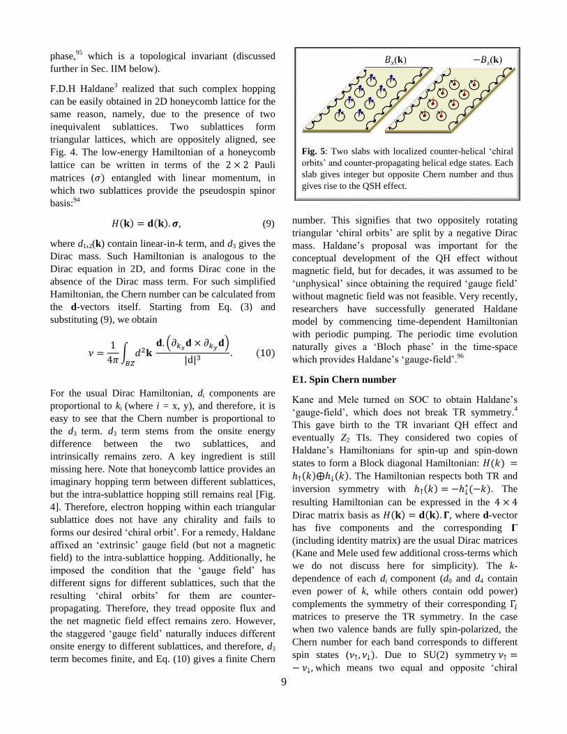
Fig. 5: Two slabs with localized counter-helical ‘chiral

orbits’ and counter-propagating helical edge states. Each

slab gives integer but opposite Chern number and thus

gives rise to the QSH effect.

10

orbits’ are stabilized due to the spin-momentum

locking, as shown in Fig. 5. Therefore the total Chern

number 𝜈 = 𝜈↑ + 𝜈↓ vanishes, while their difference,

namely spin Chern number, 𝜈𝑠 = 𝜈↑ − 𝜈↓, become

finite. Therefore, according to Kane and Mele, there is

no charge pumping to the edge, but there is a net spin

pumping, and hence they refer the corresponding state

as QSH effect.

Bernevig, Hughes, Zhang (BHZ) predicted that the

quantum well (QW) states arising in the HgTe/CdTe

heterostucture commence 2D QSH insulator above

some critical thickness.9 They realized that the band

structure for HgTe and CdTe are completely inverted

across the Fermi level. In particular, the SOC split

bands with Γ8 and Γ6 symmetries, respectively,

constitute conduction and valence bands in HgTe,

while they form valence and conduction bands in

CdTe. Therefore, if we derive a 2 label Hamiltonian

and expresses in terms of Pauli matrices as in Eq. (9),

we immediately find that the Dirac mass 𝑑3 < 0 for

HgTe and 𝑑3 > 0 for CdTe. Therefore, if one makes

an HgTe/CdTe heterostructure, at their boundary 𝑑3

must vanish, which means gapless Dirac fermions

emerge here. Based on this idea, they proposed a 4 × 4

Hamiltonian using the Kramers pairs of Γ8 and Γ6

levels. The Hamiltonian is also block diagonal with

each block representing different spin state as in the

Kane-Mele model. The Dirac mass inversion (which is

same as band inversion or parity inversion as we will

discuss in Sec. IIG below) guarantees that each block

gives equal but opposite Chern number, and QSH

insulator arises. Due to the block diagonal nature of

the mode, it is popularly known as half-BHZ model.

When two spin states cannot be separated to assign

individual Chern number, the present method does not

work. Kane and Mele proposed more rigorous method

to calculate the Z2 invariant using TR ‘polarization’

which is discussed in Sec. IIF. As we will go along,

we will learn more techniques and interpretations of

various topological invariances.

E2. Mirror Chern number

In the cases, where the band inversion occurs at non-

TR symmetric points, a distinct topological invariant

can be obtained if the system possess mirror

symmetry.8,21,53 Let us consider a case where

𝐤𝑚 represents a mirror plane in the BZ with the

corresponding mirror operator (ℳ) defined by

[𝐻(𝐤𝑚), ℳ] = 0. In such a case, the mirror plane can

be decomposed into two subspaces, denoted by ±ℳ.

Then, as in the case of half-BHZ model, the present

Hamiltonian on the mirror plane can be split into two

blocks, coming from two sub-space as 𝐻(𝐤𝑚) =

ℎ+𝑚(𝐤𝑚)⨁ℎ−𝑚(𝐤𝑚). Each block (ℎ±𝑚) gives equal

but opposite Chern number (due to TR symmetry).

Therefore, their difference 𝜈𝑚 = (𝜈+𝑚 − 𝜈−𝑚)/2

leads to a finite value, called mirror Chern number.

The corresponding TI family is refereed as topological

crystalline insulator.21

Given that the low-energy Hamiltonian here has mirror

symmetry, the leading term in the edge state will have

even power in momentum along this direction. Let us

consider an example of a mirror plane at kx = 0, which

dictates 𝐻(𝑘𝑥 , 𝑘𝑦, 𝑘𝑧) = 𝐻(−𝑘𝑥 , 𝑘𝑦, 𝑘𝑧). Since a

linear term in kx violates this condition, it will drop out

from the Hamiltonian. Therefore, the corresponding

surface state will be quadratic. Along other directions

lacking a mirror symmetry, the edge/surface state can

be linear in momentum. In fact, the surface states of

the topological crystalline insulator Sn1-xPbxTe,81 contain both quadratic and linear bands.

F. Z2 invariant and time-reversal polarization

In the case of TR breaking IQH insulator, Chern

number can take any arbitrary value. However, this is

not the case for TR invariant TIs. For such cases, spin

or mirror Chern number can take only 0 or 1 (mod 2)

value, and thus the topological invariant is represented

by a more general Z2 invariant.4,6 Z2 invariant becomes

equal to spin or mirror Chern number in the cases the

latter are defined, but there exists other methods of

evaluating it. Although spin and mirror Chern numbers

are observables via QH effect, Z2 invariant is not a

directly measurable quantity in the bulk, and is often

diagnosed by the observation of topological surface

state.

For TR symmetric cases, Kramers degeneracy at the

TR invariant k-points dramatically reduces the full

momentum space calculations into only TR invariant

k-points. The antiunitary TR operator 𝛩 imposes the

symmetry in the Hamiltonian as 𝛩𝐻∗(𝐤)𝛩−1 =

𝐻(−𝐤). Let us consider a system where the spin-

rotational symmetry is broken, say due to SOC,

without breaking the TR symmetry as 𝛩|𝐤, ↑⟩ =

11

|−𝐤, ↓⟩. The high-symmetric points 𝐤𝑠∗, which are

invariant under TR symmetry [e.g. (0,0,0), (π,0,0),

(0,π,0), (π, π,0), (π, π, π), etc in a cubic lattice in Fig.

6] are special. Here 𝐤𝑠∗ and −𝐤𝑠

∗ points are the same

[up to a reciprocal lattice vector: 𝐤𝑠∗ = −𝐤𝑠

∗ + 𝐆], so

they must be spin degenerate. This is called the

Kramers’ degeneracy.

Among many methods available for the evaluation of

the Z2 invariant, Fu-Kane-Mele method is often easier

to implement, especially in the cases where both TR

and inversion symmetries are present.7 To understand

this method, we draw analogy with some of the

properties of IQH, QSH states discussed above. In

these insulators, it is the bulk Chern number which

induces charge or spin polarizations, respectively, at

the edge. Kane and Mele asked a similar question:

what bulk property for TR invariant Z2 class can pump

a similar ‘polarization’ to the boundary. In QSH effect,

opposite spins with opposite momentum, due to SOC,

are pumped to the edge, requiring that the electron

exchanges its spin in traversing half of the BZ odd

number of times. Since opposite spins with opposite

momentum are just the TR conjugate to each other, a

more fundamental property to exchange in Z2 TI is the

TR partner of electrons. Based on this analogy, Kane,

Mele proposed a mathematical concept, called ‘TR

polarization’, in which they argued that electrons with

one Bloch wavefunction and their complex conjugate

partner are accumulated at the edge.4,97 This requires

that the electron switches its TR partner odd number of

times in traversing half of the BZ [green line in Fig.

4(a)]. [For systems with inversion symmetry, it is

equivalent to the odd number of parity, or equivalently

the Dirac mass or just simply band inversion in half of

the BZ, as discussed in Sec. IIG.]

They subsequently quantified this hypothesis4,6,7,97 by

defining the matrix element of the TI operator between

a Bloch state 𝑢𝑛(𝐤) and its TR conjugate 𝑢𝑚∗ (−𝐤) in

the Fermi sea, and construct an antisymmetric, unitary

matrix, with components

𝑤𝑚𝑛(𝐤) = ⟨𝑢𝑚(−𝐤)|𝛩|𝑢𝑛(𝐤)⟩. The determinant of

the antisymmetric matrix w is represented by the

Pfaffian as [𝑃𝑓(𝑤)]2 = det (𝑤). We define 𝑃(𝑘) =

Pf[𝑤(𝑘)]. For many TI Hamiltonians dealing with

SU(2) spin, the filled state is two-fold degenerate,

especially when inversion symmetry is present.

Therefore, the above matrix-element is a 2 × 2 matrix

in which the Pfaffian is just the off-diagonal term (the

formula for topological invariant is, however, general

to any number of filled bands).

Based on the value of P(k), the BZ can be split into the

‘even’ and ‘odd’ subspaces. In the even subspace,

𝛩|𝑢𝑛(𝐤)⟩ is proportional to |𝑢𝑚(−𝐤)⟩, making |P(k)|

= 1. In the odd subspace, 𝛩|𝑢𝑛(𝐤)⟩ is orthogonal to

|𝑢𝑚(−𝐤)⟩, implying P(k) = 0, which is important for

topological invariance. Let us assume that ±𝐤∗is a pair

of k-points, which are TR partners, where P(𝐤∗) = 0

[see Fig. 4(a)]. The phase of P(k) about each of these

points winds in opposite directions (equivalent to

having counter propagating ‘chiral orbits’ in the

momentum space). If ±𝐤∗ coincides with any TR

invariant point 𝐤𝑠∗, the two k-space ‘chiral orbits’

annihilate each other. Again if there are even number

of such points, say, ±𝐤1,2∗ , then unless 𝐤1,2

∗ are

protected by some additional symmetry, they can also

annihilate each other by scattering or perturbation. But

a single pair of ±𝐤∗ does not have the option to scatter

to another k-point, except to the corresponding ∓k-

points, which however requires the corresponding spin

to flip. Since spin flip is prohibited by the TR

symmetry, such nodal points at ±𝐤∗ remain protected

from TR invariant perturbations.

Similarity between the Berry connection formalism,

and the Pfaffian P(k) can be rigorously shown.

Differentiating w(k), and using the unitary property of

the w matrix, we obtain the Berry connection in terms

of w(k), and P(k) as7 [using Eq. (8)]

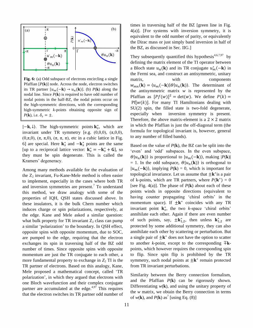
Fig. 6: (a) Odd subspace of electrons encircling a single

Pfaffian [P(k)] node. Across the node, electron switches

its TR partner [𝑢𝑚(−𝐤) → 𝑢𝑛(𝐤)]. (b) P(k) along the

nodal line. Since P(k) is required to have odd number of

nodal points in the half-BZ, the nodal points occur on

the high-symmetric directions, with the corresponding

high-symmetric k-points obtaining opposite sign of

P(k), i.e. 𝛿𝑠 = ±.

12

𝐀(𝐤) = −𝑖

2Tr[𝑤(𝐤)†∇𝐤𝑤(𝐤)] = −

𝑖

2Tr[∇𝐤log 𝑤(𝐤)]

= −𝑖

2∇𝐤log det[𝑤(𝐤)] = − 𝑖∇𝐤 log[𝑃(𝐤)] (11)

Based on this, 𝑍2 invariant can be defined by

calculating the winding number of the P(k) over a

single k-space ‘chiral orbit’, in a contour enclosing

half of the BZ (so that only either +𝐤∗ or −𝐤∗ is

included), as shown by green boundary in Fig. 4(a).

So, from Eq. (5), Z2 invariant can be evaluated as:

𝜈 =1

2𝜋𝑖∮ 𝑑𝐤

𝐶⋅ ∇𝐤 log[𝑃(𝐤) + 𝑖𝛿], (12)

where a complex term iδ is introduced to evaluate the

above integral in a complex contour plane. This

simplifies the integral into a residue problem, with

singularities occurring at the loci of P(𝐤∗) = 0.

Given that there should be an odd number of Pfaffian

nodes in half of the BZ, it is expected that the

corresponding nodes would occur on the high-

symmetric k-directions. This simply means that P(k)

should change sign odd number of times on both sides

of the nodes at the TR invariant k-points [see Fig.

4(b)]. Therefore, the calculation simply reduces to

counting the sign of P(k) at the TR invariant momenta

in the first quadrant of the BZ only. If we take the

product of the sign of the Pfaffian at all TR invariant

points, and the result comes out to be negative, then

there must be odd number of zeros in the first quadrant

of the BZ. Since [Pf(𝑤)]2 = det (𝑤), the sign of the

Pfaffian can be defined in a formal way as

𝛿𝑠 =√det [𝑤(𝐤𝑠

∗)]

Pf[𝑤(𝐤𝑠∗)]

= ±1, (13)

Therefore, in a 1D system, the TR polarization can be

defined as (−1)𝜈 = 𝛿1𝛿2, where 𝛿1, and 𝛿2 are

evaluated at the two TR invariant points. If 𝛿1, and 𝛿2

have opposite sign, we get the 𝑍2 invariant 𝜈 = 1,

which signals the non-trivial topological phase. The

formula generalizes to higher dimensions as

(−1)𝜈 = ∏ 𝛿𝑠𝑁𝑠𝑠=1 , (14)

where Ns is the total number of the TR invariant

momenta in the first quadrant of the BZ. In a 2D

square lattice, Ns = 4, while in a 3D C4 symmetric

lattice Ns= 8. If there are odd number of 𝛿𝑠 = −1 in

this k-space, the right hand side of the above equation

gives -1, which therefore yields 𝜈 = 1, a non-trivial

topological invariant. This is called the strong

topological invariant (denoted by 𝜈0). Note that for

any arbitrarily large odd number of 𝛿𝑠 = −1,

topological invariant remains 𝜈0 = 1, otherwise 0.

Therefore, unlike in IQH insulator where arbitrarily

large Chern number is possible, here one only gets two

values of 𝜈0 and the Z2 symmetry emerges.

In some cases, there can be total even number of 𝑘𝑠∗-

points with 𝛿𝑠 = −1, but they lie in different planes

(say on the 𝑘𝑥 = 0, and 𝑘𝑥 = 𝜋 planes) [see Fig. 5(c)].

Thus those 2D planes contain odd number of 𝛿𝑠 = −1,

and constitute non-trivial 2D TIs, while the 3D system

remains trivial TI. This is called the weak TI. Since in

3D, there are three orthogonal coordinate axes, there

are three weak topological invariants (𝜈1, 𝜈2, 𝜈3). Fu,

Kane, and Mele,6 thereby, introduced four Z2

invariants (𝜈0: 𝜈1𝜈2𝜈3) for 3D TIs. This part is

explained with examples in Fig. 7 and discussed

further in the following section.

G. Z2 calculation with inversion symmetry

If the system possesses inversion symmetry, in

addition to TR symmetry, calculation of topological

invariants becomes exceptionally simpler. Suppose 𝒫

is the parity operator defined by 𝒫|𝑘, ↑⟩ = |−𝑘, ↑⟩,

under which the Hamiltonian transforms as 𝐻(−𝐤) =

𝒫𝐻(𝐤)𝒫−1. Inserting 𝒫2 = 1 in the expression for

𝑤𝑚𝑛(𝐤), and employing the identity that [𝐻, 𝒫𝛩] = 0,

𝛿𝑠 parameter at the TR invariant moment 𝐤𝑠∗ can be

evaluated as7

𝛿𝑠 = ∏ 𝜉𝑚(𝐤𝑠∗)𝑁

𝑚=1 , (15)

where 𝜉𝑚(𝐤𝑠∗)=±1 is the parity eigenvalue at 𝐤𝑠

∗

defined as 𝒫|𝑢𝑚(𝐤𝑠∗)⟩ = 𝜉𝑚(𝐤𝑠

∗)|𝑢𝑚(𝐤𝑠∗)⟩. The

product is computed for N filled bands. In practice one

does not have to include all filled bands in the

calculation, rather only those bands which undergoes

band inversion at the TR invariant points. For the two

typical Dirac Hamiltonians which are expressed in

terms of 2 × 2 Pauli matrices or 4 × 4 Dirac matrices,

the parity term turns out to be 𝜎z, or Γ4 = 𝜎z⨂I2×2,

respectively. The corresponding k-dependent d-vector

component can often be written as 𝑑4(𝐤𝑠∗) =

(휀1(𝐤𝑠∗) − 휀2(𝐤𝑠

∗))/2, where 휀1,2(𝐤𝑠∗) are the

conduction and valence bands near the Fermi level.

Therefore, the parity eigenvalue of the Hamiltonian is

determined simply by 𝜉𝑚(𝐤𝑠∗) = sgn[𝑑4(𝐤𝑠

∗)]. For

13

systems with both inversion and TR symmetries, the

Z2 invariant is obtained by simply counting the number

of band inversion at the high-symmetric momenta as:

(−1)𝜈 = ∏ sgn[휀1(𝐤𝑠∗) − 휀2(𝐤𝑠

∗)]𝑁𝑠𝑠=1 . (16)

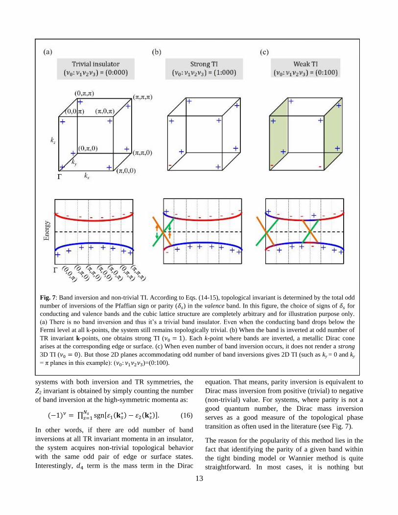
In other words, if there are odd number of band

inversions at all TR invariant momenta in an insulator,

the system acquires non-trivial topological behavior

with the same odd pair of edge or surface states.

Interestingly, 𝑑4 term is the mass term in the Dirac

equation. That means, parity inversion is equivalent to

Dirac mass inversion from positive (trivial) to negative

(non-trivial) value. For systems, where parity is not a

good quantum number, the Dirac mass inversion

serves as a good measure of the topological phase

transition as often used in the literature (see Fig. 7).

The reason for the popularity of this method lies in the

fact that identifying the parity of a given band within

the tight binding model or Wannier method is quite

straightforward. In most cases, it is nothing but

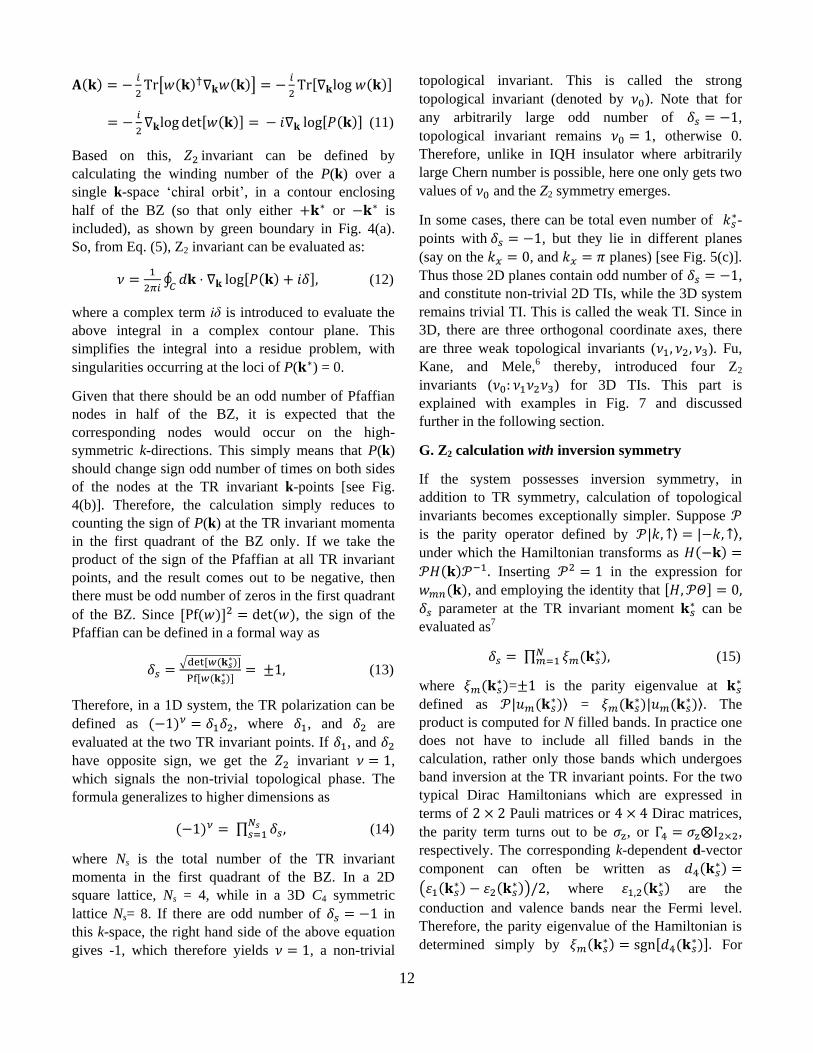
Fig. 7: Band inversion and non-trivial TI. According to Eqs. (14-15), topological invariant is determined by the total odd

number of inversions of the Pfaffian sign or parity (𝛿𝑠) in the valence band. In this figure, the choice of signs of 𝛿𝑠 for

conducting and valence bands and the cubic lattice structure are completely arbitrary and for illustration purpose only.

(a) There is no band inversion and thus it’s a trivial band insulator. Even when the conducting band drops below the

Fermi level at all k-points, the system still remains topologically trivial. (b) When the band is inverted at odd number of

TR invariant k-points, one obtains strong TI (𝜈0 = 1). Each k-point where bands are inverted, a metallic Dirac cone

arises at the corresponding edge or surface. (c) When even number of band inversion occurs, it does not render a strong

3D TI (𝜈0 = 0). But those 2D planes accommodating odd number of band inversions gives 2D TI (such as ky = 0 and ky

= π planes in this example): (𝜈0: 𝜈1𝜈2𝜈3)=(0:100).

14

knowing the orbital character of the valence and

conduction bands. So band inversion simply refers to

switching orbital character between these two

classes.16,17,81 However, band inversion does not mean

that an orbital entirely switches its position between

conduction and valence bands at all k-points, rather it

has to be done only at odd number of TR k-points, and

not at other k-points. For example, in Fig. 7(a), if the

odd parity conduction band drops fully below the

Fermi level, the system still remains topologically

trivial. This means the inter-orbital overlap matrix-

element has to be strongly momentum dependent.

Simple local inter-orbital hopping or crystal field

splitting or onsite interactions such as Hubbard U or

Hund’s coupling are often not adequate to commence

such a k-dependent band inversion. Spin-momentum

locking due to SOC does this job in most of the known

TIs.

Some caution has to be taken for the cases when a

band at a given TR invariant k-point is not fully

orbitally polarized, rather it contains a mixture of both

even and odd orbitals. In such cases, the band

inversion mechanism cannot be considered as

conclusive. In this context, a term called band

inversion strength is often used which measures the

amount of orbital weight is exchanged between the

conduction and valence bands. Band inversion strength

is also used as a measure the Dirac gap at the TR k-

points [see, for example, Ref. 20]. Associated with the

orbital weight transfer, the band topology also changes

in this process. For example, if the top of the valence

band has an upward curvature, it changes to a

downward curvature around the TR k-point after the

band inversion. This structure is sometimes referred as

‘dent’ in the band structure, which is seen in the DFT

band structure, as well in the experimental data.5,65

Three representative examples for trivial, strong, and

weak TIs are given in Fig. 7. Owing to TR symmetry,

it is sufficient to consider only the first quadrant of the

BZ to count the number of band inversions, since the

other k-points are related to them by TR symmetry. As

mentioned earlier, if the conduction and valence bands

possess the same parity at all k-points, but different

among them, Eq. (15) suggests that it is a trivial

topological insulator, or not a topological insulator

[Fig. 7(a)]. Fig. 7(b) depicts the case of a single band

inversion at the Γ-point, indicating a strong TI (𝜈0 =

1). In this case, all three surfaces of the lattice possess

Dirac cones with the vertex of the cone lying at the

same k-point where the band inversion has occurred. If

the band inversions occur even number of times in the

first quadrant, a weak TI can be obtained if one or

more BZ sides possess odd number of band inversions.

For example, in Fig. 7(c), we consider the case of two

band inversions at the Γ- and at (π,0,0)-points, yielding

𝜈0 = 0. But the kx = 0 and kx = π-planes contain only

single band inversion, and the corresponding

topological invariant becomes 𝜈1 = 1, while 𝜈2,3 = 0.

A weak 3D TI can be thought of a stacking of 2D TIs,

each having edge states. Since there are even number

of Dirac cones here, scattering between them due to

impurity or correlation can open a gap, and thus they

are not topologically protected. Thus this state is

refereed as weak topological insulator.

Each TR invariant k-point possessing a band inversion

hosts an edge state. No matter how many band

inversions occur, as long as it is odd in number, we

have the same Z2 invariant 𝜈0 = 1, but the

corresponding number of Dirac cones at the edge is

equal to the number of band inversions. This is in

contrast to the Chern insulator where the bulk

topological invariant dictates the number of surface

state.

H. Z2 calculation without inversion symmetry

Subsequently, Fu and Kane have generalized the Z2

calculation for systems without inversion symmetry97:

𝜈 = 1

2𝜋[∮ 𝐴𝑛(𝐤)𝑑𝑘 − ∫ 𝐹𝑛(𝐤)

𝜏𝑑2𝑘

𝑑𝜏], (17)

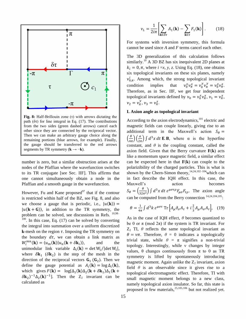
τ is half of the BZ one in which the Berry curvature is

to be computed, while 𝑑𝜏 is the boundary where the

integral of the Berry connection is to be calculated (see

Fig. 8). The difference between Eq. (17) and Eq. (5) is

that here an additional surface integral over the Berry

connection is present. This term appears in the process

of gauge fixing as follows.

In systems with finite Chern number, the center of the

cyclotron orbit or ‘chiral orbit’ poses an obstruction to

smoothly affix a gauge to the wavefunction. Because,

the phase of the wavefunction is supposed to acquire a

discontinuity at the center of the orbit to commence

finite phase winding or Chern number. If the

wavefunction has a smooth gauge at all k-points, both

A and F acquire the same gauge, yielding 𝜈 = 0 by

Stokes’ theorem. For Z2 TIs, although the Chern

15

number is zero, but a similar obstruction arises at the

nodes of the Pfaffian where the wavefunction switches

to its TR conjugate [see Sec. IIF]. This affirms that

one cannot simultaneously obtain a node in the

Pfaffian and a smooth gauge in the wavefunction.

However, Fu and Kane proposed97 that if the contour

is restricted within half of the BZ, see Fig. 8, and also

we choose a gauge that is periodic, i.e., |𝑢(𝐤)⟩ =

|𝑢(𝐤 + 𝐆)⟩, in addition to the TR symmetry, the

problem can be solved, see discussions in Refs. 10,98–

100. In this case, Eq. (17) can be solved by converting

the integral into summation over a uniform discretized

k-mesh on the region 𝜏. Imposing the TR symmetry on

the boundary 𝑑𝜏, we can obtain a link matrix as

𝑊𝑖𝑚𝑛(𝐤) = ⟨𝑢𝑚(𝐤)|𝑢𝑛(𝐤 + 𝛿𝐤𝑖)⟩, and the

unimodular link variable Δ𝑖(𝐤) = det W𝑖 |det W𝑖|⁄ ,

where 𝛿𝐤1 (𝛿𝐤2) is the step of the mesh in the

direction of the reciprocal vectors 𝐆1 (𝐆2). Then we

define the gauge potential as 𝐴𝑖(𝐤) = log Δ𝑖(𝐤),

which gives 𝐹(𝐤) = log [Δ1(𝐤)Δ2(𝐤 + 𝛿𝐤1)Δ1(𝐤 +

𝛿𝐤2)−1Δ2(𝐤)−1]. Then the Z2 invariant can be

calculated as

𝜈𝐿 =1

2𝑖𝜋[ ∑ 𝐴1(𝐤) − ∑ 𝐹1(𝐤)

𝐤∈𝜏𝐤∈𝛿𝜏

] . (18)

For systems with inversion symmetry, this formula

cannot be used since A and F terms cancel each other.

The 3D generalization of this calculation follows

similarly.10 A 3D BZ has six inequivalent 2D planes at

𝑘𝑖 = 0, 𝜋, where i =x, y, z. Using Eq. (18), one obtains

six topological invariants on these six planes, namely

𝜈0,𝜋𝑖 . Among which, the strong topological invariant

condition implies that 𝜈0𝑥𝜈𝜋

𝑥 = 𝜈0𝑦

𝜈𝜋𝑦

= 𝜈0𝑧𝜈𝜋

𝑧.

Therefore, as in Sec. IIF, we get four independent

topological invariants defined by 𝜈0 = 𝜈0𝑥𝜈𝜋

𝑥, 𝜈1 = 𝜈𝜋𝑥,

𝜈2 = 𝜈𝜋𝑦

, 𝜈3 = 𝜈𝜋𝑧.

I. Axion angle as topological invariant

According to the axion electrodynamics,101 electric and

magnetic fields can couple linearly, giving rise to an

additional term in the Maxwell’s action 𝑆𝜃 =

(𝜃

4𝜋) (

𝛼

2𝜋) ∫ 𝑑3𝑥 𝑑𝑡 𝐄. 𝐁, where α is the hyperfine

constant, and θ is the coupling constant, called the

axion field. Given that the Berry curvature F(k) acts

like a momentum space magnetic field, a similar effect

can be expected here in that F(k) can couple to the

polarizibility of the charged particles. This is what is

shown by the Chern-Simon theory,14,24,102–104which can

in fact describe the IQH effect. In this case, the

Maxwell’s action becomes

𝑆𝜃 = (𝜃

32𝜋2) ∫ 𝑑3𝑥 𝑑𝑡 휀𝜇𝜎𝜏𝜌𝐹𝜇𝜎𝐹𝜏𝜌. The axion angle

can be computed from the Berry connection 14,24,104,105:

𝜃 =1

4𝜋∫ 𝑑3𝑘 휀𝜇𝜎𝜏 Tr [𝐴𝜇𝜕𝜎𝐴𝜏 + 𝑖

2

3𝐴𝜇𝐴𝜎𝐴𝜏], (19)

As in the case of IQH effect, θ becomes quantized to

be 0 or π (mod 2π) if the system is TR invariant. For

Z2 TI, θ reflects the same topological invariant as

𝜃 = 𝜈𝜋. Therefore, θ = 0 indicates a topologically

trivial state, while θ = π signifies a non-trivial

topology. Interestingly, while ν changes by integer

values, θ changes continuously from π to 0 as TR

symmetry is lifted by spontaneously introducing

magnetic moment. Again unlike the Z2 invariant, axion

field θ is an observable since it gives rise to a

topological electromagnetic effect. Therefore, TI with

small magnetic moment belongs to a new class,

namely topological axion insulator. So far, this state is

proposed in few materials,25,105,106 but not realized yet.

Fig. 8: Half-Brillouin zone (τ) with arrows dictating the

path (δτ) for line integral in Eq. (17). The contributions

from the two sides (green dashed arrows) cancel each

other since they are connected by the reciprocal vector.

Then we can make an arbitrary gauge choice along the

remaining portions (blue arrows, for example). Finally,

the gauge should be transferred to the red arrows

segments by TR symmetry (k → −k).

16

As the magnetic moment is further increased, another

class of TI, called quantum anomalous Hall (QAH)

insulator, may arise if the system undergoes a similar

band inversion. Here, a Z2 classification is destroyed,

and the system can in principle possess arbitrarily

large value of Chern number. QAH state is proposed

and realized in various engineered structures,61,107–109

and LaX (X=Br, Cl, I) is the only family predicted so

far as intrinsic QAH insulator.62

J. Topological invariant for interacting fermions

For non-interacting systems, the topological invariant

can be extracted from the Kubo formula for the Hall

conductivity in 2D [Eq. (3)]. For interacting systems,

one can follow the same strategy.89,110 For such

systems, a single-particle wavefunction cannot be

defined and thus we start from a different Kubo

formula for interacting systems as 𝜎𝑥𝑦 =

𝑒2

ℏ Im

𝜕

𝜕𝜔 𝛫(𝜔 + 𝑖𝛿). The current-current correlation

kernel 𝛫(𝜔 + 𝑖𝛿) can be expressed in terms of the

interacting Green’s function 𝐺(𝑘, 𝑖𝜔) as

𝛫(𝑖𝜔) = −1

ΩBZ𝛽∑ Tr[𝑣𝑥𝐺(𝑘, 𝑖𝜔 + 𝑖𝜈)𝑣𝑦𝐺(𝑘, 𝑖𝜔)]

𝑘,𝑖𝜈

,

(20)

where ΩBZ is the phase space volume, 𝛽 = 1/𝑘𝐵𝑇,

and the velocity vertices are 𝑣𝑖 (𝐤) = 𝜕𝐻(𝐤) 𝜕𝑘𝑖⁄ .

For (2+1)D systems, the vertex can be expressed

within the Ward identity as 𝑣𝑖(𝑝) = 𝜕𝐺−1(𝑝) 𝜕𝑝𝑖⁄ ,

where 𝑝 = (𝐤, 𝑖𝜔). Integrating over the (2+1)D phase

space volume, we obtain a similar topological

invariant (Chern number) in terms of generalized

Green’s function as90

𝜈 =𝜋

6∫

𝑑3𝑝

(2𝜋)3Tr [휀𝜇𝜌𝜎 𝐺

𝜕𝐺−1

𝜕𝑝𝜇𝐺

𝜕𝐺−1

𝜕𝑝𝜌𝐺

𝜕𝐺−1

𝜕𝑝𝜎]

.

(21)

Extension to higher dimensions follows the same

procedure, in which the number of vertices is equal to

the dimension of the system.14,111 Clearly, Eq. (21) is

also applicable to non-interacting Green’s function

𝐺0(𝑘, 𝑖𝜔) = (𝑖𝜔 − 𝐻(𝑘))−1. In the multi-orbital

systems, corresponding Green’s function is a tensor.

Electron-electron interaction or disorder effect can be

incorporated within the Dyson, or the T - matrix

formalism, among others, giving a generalized

formalism 𝐺(𝑘, 𝑖𝜔)−1 = 𝐺0(𝑘, 𝑖𝜔)−1 − Σ(𝑘, 𝑖𝜔),

where Σ is the self-energy correction. Dynamical

mean-field theory (DMFT), and momentum-resolved

density fluctuation (MRDF) theory112–117are two

widely used methods to explore the dynamical

correction effects. The latter method has an added

advantage of incorporating the full momentum

dependence of the correlation effects. For many

systems such as transition metal oxides,112,115 and di-

chalcogenides,114 intermetallics, lanthanum and

actinide compounds,113,116 the momentum dependence

of the electron-correlation is significantly strong,

which can lead to a characteristic change in the Berry

curvature F(𝐤). These features can be captured within

the MRDF method.

K. Topological invariants for superconductors

Superconductivity is a correlated phenomenon which

arises due to the condensation of electron-electron pair

(Cooper pair) in the low-energy spectrum. Within the

mean-field theory, the corresponding Hamiltonian can

be casted into a single particle (quasiparticle)

Hamiltonian in which the superconductivity opens a

band gap at the Fermi level. Therefore, although in the

two electrons picture, the system is superconducting

(SC), in the single electron effective model it

represents an insulator (assuming the SC gap opens

everywhere on the Fermi surface). Interestingly, fully

gapped superconductor, and topological insulator

share an analogous Hamiltonian, and thus many of the

topological concepts also applies in the former

case.22,83,118–123 The single-band Hamiltonian for a

superconductor can be expressed exactly by Eq. (9),

with 𝑑3 = 휀(𝐤), 𝑑1,2 are the real and imaginary parts

of the SC gap, ∆(𝐤). Furthermore, the owing to the

criterion for the formation of ‘chiral orbit’ or ‘chiral

vortex’, the SC gap must be a chiral pairing symmetry,

which is often obtained in p-wave superconductors

(for spinful superconductors, this condition can be

relaxed if SOC is present23). The chiral p-wave

superconductors have odd parity gap symmetry and

breaks TR symmetry. In such a case, the topological

invariant is obtained by the sum of the first Chern

number (𝜈𝑛) on each band weighted by the sign of the

gap as22,23,118,124

𝒩 =1

2∑ 𝜈𝑛𝑛 sgn(𝛥𝑛𝒌). (22)

For spinful case, TR invariant topological

superconductor can be obtained if the pairings

17

⟨𝜓𝑘↑† 𝜓−𝑘↑

† ⟩ and ⟨𝜓𝑘↓† 𝜓−𝑘↓

† ⟩ have opposite chirality, i.e.,

Δ↑↑ = 𝑝𝑥 + 𝑖𝑝𝑦, and Δ↓↓ = 𝑝𝑥 − 𝑖𝑝𝑦. Here again if the

corresponding 4 × 4 Hamiltonian can be split into the

block diagonals, as in the case of half-BHZ model for

QSH insulator, we can apply the same Chern number

calculation to evaluate the topological invariant. Due

to the associated particle-hole symmetry, the zero

energy boundary modes must be a Majorana

mode,83,119,123 which means, its eigenstate must be real.

L. Adiabatic continuity

Adiabatic continuation is a simple and powerful tool to

identify a non-trivial TI with reference to another

known TI, if both these systems are adiabatically

connected. Here ‘adiabatic connection’ simply means

that as one transforms a non-trivial TI ‘A’ into another

material ‘B’ by continuously changing the atomic

number of the constituent elements, the bulk band gap

of the ‘A’ system does not close and reopen in this

whole process, then they are adiabatically connected

or belong to the same non-trivial TI class.

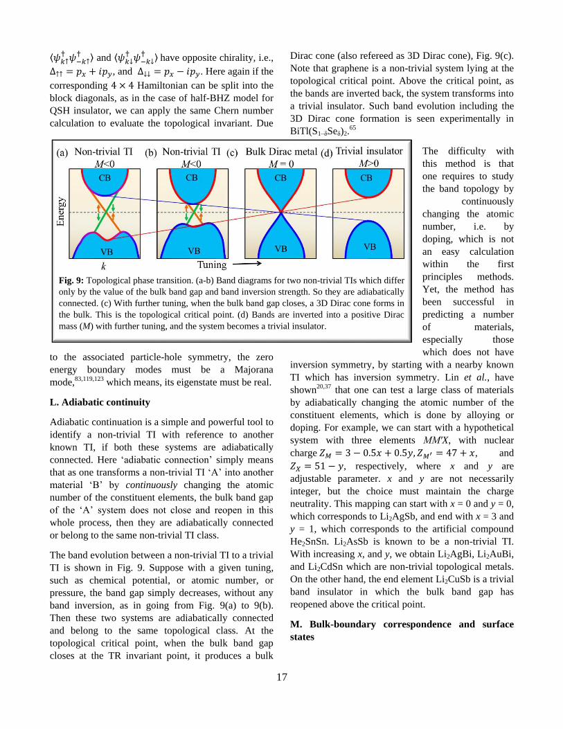
The band evolution between a non-trivial TI to a trivial

TI is shown in Fig. 9. Suppose with a given tuning,

such as chemical potential, or atomic number, or

pressure, the band gap simply decreases, without any

band inversion, as in going from Fig. 9(a) to 9(b).

Then these two systems are adiabatically connected

and belong to the same topological class. At the

topological critical point, when the bulk band gap

closes at the TR invariant point, it produces a bulk

Dirac cone (also refereed as 3D Dirac cone), Fig. 9(c).

Note that graphene is a non-trivial system lying at the

topological critical point. Above the critical point, as

the bands are inverted back, the system transforms into

a trivial insulator. Such band evolution including the

3D Dirac cone formation is seen experimentally in

BiTl(S1–δSeδ)2.65

The difficulty with

this method is that

one requires to study

the band topology by

continuously

changing the atomic

number, i.e. by

doping, which is not

an easy calculation

within the first

principles methods.

Yet, the method has

been successful in

predicting a number

of materials,

especially those

which does not have

inversion symmetry, by starting with a nearby known

TI which has inversion symmetry. Lin et al., have

shown20,37 that one can test a large class of materials

by adiabatically changing the atomic number of the

constituent elements, which is done by alloying or

doping. For example, we can start with a hypothetical

system with three elements MM′X, with nuclear

charge 𝑍𝑀 = 3 − 0.5𝑥 + 0.5𝑦, 𝑍𝑀′ = 47 + 𝑥, and

𝑍𝑋 = 51 − 𝑦, respectively, where x and y are

adjustable parameter. x and y are not necessarily

integer, but the choice must maintain the charge

neutrality. This mapping can start with x = 0 and y = 0,

which corresponds to Li2AgSb, and end with x = 3 and

y = 1, which corresponds to the artificial compound

He2SnSn. Li2AsSb is known to be a non-trivial TI.

With increasing x, and y, we obtain Li2AgBi, Li2AuBi,

and Li2CdSn which are non-trivial topological metals.

On the other hand, the end element Li2CuSb is a trivial

band insulator in which the bulk band gap has

reopened above the critical point.

M. Bulk-boundary correspondence and surface

states

Fig. 9: Topological phase transition. (a-b) Band diagrams for two non-trivial TIs which differ

only by the value of the bulk band gap and band inversion strength. So they are adiabatically

connected. (c) With further tuning, when the bulk band gap closes, a 3D Dirac cone forms in

the bulk. This is the topological critical point. (d) Bands are inverted into a positive Dirac

mass (M) with further tuning, and the system becomes a trivial insulator.

18

Spontaneous (continuous) symmetry breaking leads to

gapless Goldstone mode in the corresponding

excitation spectrum. For example, the spin rotational

symmetry breaking in quantum magnets leads to

gapless magnons in the spin excitation spectrum, or

the translational symmetry breaking in the formation

of a lattice renders gapless phonon mode (acoustic

modes). Similarly, as the cyclotron orbits or ‘chiral

orbits’ become periodically arranged in a lattice

(creating a Gaussian curvature), breaking the

translational symmetry, which is associated with the

emergence of non-trivial bulk topology, it manifests

into gapless edge states at the boundary. Although a

rigorous calculation to validate this premise is yet not

explored, however, the application of Goldstone

theory for the realization of bulk-boundary

correspondence can be intriguing. For example,

electromagnetic response of TIs stipulates two

dynamical axion modes, one of them is gapless

Goldstone-like mode, and another is Higgs-like

gapped mode, as shown in earlier calculation.104

According to the bulk-boundary correspondence of TI,

the bulk topological invariant dictates the number and

characteristics of edge states at the boundary. For the

case of IQH effect, the Chern number N prescribes N

chiral edge states. For the spin or mirror Chern

numbers, edge states form in pair; for example, N spin

Chern number has 2N counter-propagating chiral edge

states. The same principle also applies to Z2

topological invariant with some modifications. Kane-

Mele proposed that for TR invariant Z2 TI, the TR

partners are accumulated at different sides leading to

the ‘TR polarization’. In the presence of additional

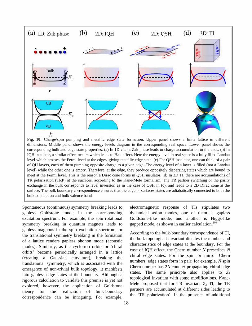
Fig. 10: Charge/spin pumping and metallic edge state formation. Upper panel shows a finite lattice in different

dimensions. Middle panel shows the energy levels diagram in the corresponding real space. Lower panel shows the

corresponding bulk and edge state properties. (a) In 1D chain, Zak phase leads to charge accumulation to the ends. (b) In

IQH insulator, a similar effect occurs which leads to Hall effect. Here the energy level in real space is a fully filled Landau

level which crosses the Fermi level at the edges, giving metallic edge state. (c) For QSH insulator, one can think of a pair

of QH layers, each of them pumping opposite charge to a given edge. The energy level of a layer is filled (not a Landau

level) while the other one is empty. Therefore, at the edge, they produce oppositely dispersing states which are bound to

meet at the Fermi level. This is the reason a Dirac cone forms in QSH insulator. (d) In 3D TI, there are accumulations of

TR polarization (TRP) at the surfaces, according to the Kane-Mele formalism. The TR partner switching or the parity

exchange in the bulk corresponds to level inversion as in the case of QSH in (c), and leads to a 2D Dirac cone at the

surface. The bulk boundary correspondence ensures that the edge or surfaces states are adiabatically connected to both the

bulk conduction and bulk valence bands.

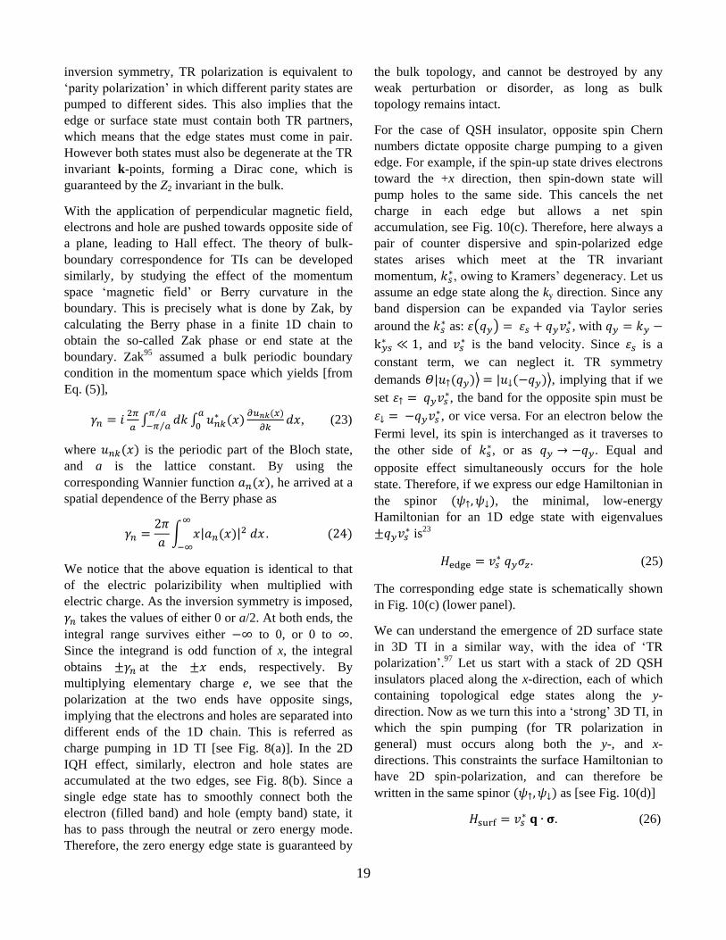
19

inversion symmetry, TR polarization is equivalent to

‘parity polarization’ in which different parity states are

pumped to different sides. This also implies that the

edge or surface state must contain both TR partners,

which means that the edge states must come in pair.

However both states must also be degenerate at the TR

invariant k-points, forming a Dirac cone, which is

guaranteed by the Z2 invariant in the bulk.

With the application of perpendicular magnetic field,

electrons and hole are pushed towards opposite side of

a plane, leading to Hall effect. The theory of bulk-

boundary correspondence for TIs can be developed

similarly, by studying the effect of the momentum

space ‘magnetic field’ or Berry curvature in the

boundary. This is precisely what is done by Zak, by

calculating the Berry phase in a finite 1D chain to

obtain the so-called Zak phase or end state at the

boundary. Zak95 assumed a bulk periodic boundary

condition in the momentum space which yields [from

Eq. (5)],

𝛾𝑛 = 𝑖2𝜋

𝑎∫ 𝑑𝑘 ∫ 𝑢𝑛𝑘

∗ (𝑥)𝜕𝑢𝑛𝑘(𝑥)

𝜕𝑘

𝑎

0𝑑𝑥

𝜋 𝑎⁄

−𝜋 𝑎⁄, (23)

where 𝑢𝑛𝑘(𝑥) is the periodic part of the Bloch state,

and a is the lattice constant. By using the

corresponding Wannier function 𝑎𝑛(𝑥), he arrived at a

spatial dependence of the Berry phase as

𝛾𝑛 =2𝜋

𝑎∫ 𝑥|𝑎𝑛(𝑥)|2 𝑑𝑥

∞

−∞

. (24)

We notice that the above equation is identical to that

of the electric polarizibility when multiplied with

electric charge. As the inversion symmetry is imposed,

𝛾𝑛 takes the values of either 0 or a/2. At both ends, the

integral range survives either −∞ to 0, or 0 to ∞.

Since the integrand is odd function of x, the integral

obtains ±𝛾𝑛 at the ±𝑥 ends, respectively. By

multiplying elementary charge e, we see that the

polarization at the two ends have opposite sings,

implying that the electrons and holes are separated into

different ends of the 1D chain. This is referred as

charge pumping in 1D TI [see Fig. 8(a)]. In the 2D

IQH effect, similarly, electron and hole states are

accumulated at the two edges, see Fig. 8(b). Since a

single edge state has to smoothly connect both the

electron (filled band) and hole (empty band) state, it

has to pass through the neutral or zero energy mode.

Therefore, the zero energy edge state is guaranteed by

the bulk topology, and cannot be destroyed by any

weak perturbation or disorder, as long as bulk

topology remains intact.

For the case of QSH insulator, opposite spin Chern

numbers dictate opposite charge pumping to a given

edge. For example, if the spin-up state drives electrons

toward the +x direction, then spin-down state will

pump holes to the same side. This cancels the net

charge in each edge but allows a net spin

accumulation, see Fig. 10(c). Therefore, here always a

pair of counter dispersive and spin-polarized edge

states arises which meet at the TR invariant

momentum, 𝑘𝑠∗, owing to Kramers’ degeneracy. Let us

assume an edge state along the ky direction. Since any

band dispersion can be expanded via Taylor series

around the 𝑘𝑠∗ as: 휀(𝑞𝑦) = 휀𝑠 + 𝑞𝑦𝑣𝑠

∗, with 𝑞𝑦 = 𝑘𝑦 −

k𝑦𝑠∗ ≪ 1, and 𝑣𝑠

∗ is the band velocity. Since 휀𝑠 is a

constant term, we can neglect it. TR symmetry

demands 𝛩|𝑢↑(𝑞𝑦)⟩ = |𝑢↓(−𝑞𝑦)⟩, implying that if we

set 휀↑ = 𝑞𝑦𝑣𝑠∗, the band for the opposite spin must be

휀↓ = −𝑞𝑦𝑣𝑠∗, or vice versa. For an electron below the

Fermi level, its spin is interchanged as it traverses to

the other side of 𝑘s∗, or as 𝑞𝑦 → −𝑞𝑦. Equal and

opposite effect simultaneously occurs for the hole

state. Therefore, if we express our edge Hamiltonian in

the spinor (𝜓↑, 𝜓↓), the minimal, low-energy

Hamiltonian for an 1D edge state with eigenvalues

±𝑞𝑦𝑣𝑠∗ is23

𝐻edge = 𝑣𝑠∗ 𝑞𝑦𝜎𝑧 . (25)

The corresponding edge state is schematically shown

in Fig. 10(c) (lower panel).

We can understand the emergence of 2D surface state

in 3D TI in a similar way, with the idea of ‘TR

polarization’.97 Let us start with a stack of 2D QSH

insulators placed along the x-direction, each of which

containing topological edge states along the y-

direction. Now as we turn this into a ‘strong’ 3D TI, in

which the spin pumping (for TR polarization in

general) must occurs along both the y-, and x-

directions. This constraints the surface Hamiltonian to

have 2D spin-polarization, and can therefore be

written in the same spinor (𝜓↑, 𝜓↓) as [see Fig. 10(d)]

𝐻surf = 𝑣𝑠∗ 𝐪 ∙ 𝛔. (26)

20

Note that this surface Hamiltonian is very analogous to

the Rashba-type SOC ℎ𝑅 = 𝑘2 2𝑚⁄ I2×2 ±

𝛼𝑅(𝐪 × 𝛔), where 𝛼𝑅 is the SOC strength and the

other symbols have the usual meanings. Indeed, owing

to the loss of inversion symmetry at the surface, the

surface states actually originate from the Rashba-type

SOC, with a crucial difference. In the topological

surface state, the kinetic energy of each spin (𝑘2 2𝑚⁄ )

is much smaller compared to the SOC strength,

𝑘2 2𝑚⁄ ≪ 𝛼𝑅 . This is a manifestation of the bulk-

boundary correspondence of the TI. For the Rashba-

band, in Fig. 11(a), each spin band bends backward

away from the TR momentum as the kinetic energy

term dominates over SOC term at higher momenta.

The Rashba-bands are not required to connect to the

bulk states at all. On the other hand, topological

surface states are required to adiabatically connect to

both the bulk conduction and valence bands, and thus

they cannot bend backward and rather disperse

monotonically across the bulk insulating gap. This is

illustrated in Fig. 11(b). It is obvious that all

edge/surface states are not topological surface state.

More importantly, even in a TI, all surface states are

not necessarily topological surface state as well.125 A

topological surface state must have a Dirac cone at the

TR point where band inversion occurred in the bulk

state and it also has to connect both the bulk valence

and conduction states. There might be situation where

an apparently isolated topological state may arise

which is not connecting any other state.126 Here

however, if one studies the eigenvector or weight of

the band, it may appear that the weight has changed

from surface to bulk as one moves away from the

Dirac node.

III. Engineering topological insulators

The above introduction highlights some key

ingredients universally relating different TI families.

The foremost ingredient is that electrons must contain

a chirality, i.e., complex hopping term, which is

obtained either via applied magnetic field (Pierels

phase), or in bipartite lattice (such as SSH,15 or

graphene lattice,94

), or via SOC, or in orbital selective

lattice,16,17 or even by artificial gauge fields as often

done in optical lattice systems.96,127 These chiral states

must also form cyclotron or ‘chiral orbits’, with or

without magnetic field. The ‘chiral orbits’ naturally

produces a k-space ‘magnetic fields’, or Berry

curvature. As these ‘chiral orbits’ are arranged in a 2D

lattice, the system can be represented by a Gaussian

curvature (torus as in the case of IQH system), each

threading counter propagating integer multiple of

quantum flux of the Berry curvature. In Sec. IIC, we

also discussed that the ‘chiral orbits’ does not have to

be formed in a physical parameter space, such as real

or momentum space, but can also be formed in any

generalized parameter space as long as they obey

periodic boundary conditions. For such case, the Hall

conductance can be precisely calculated. Therefore,

for the cases where the two chiral states can be fully

separated in the Hamiltonian (as in the case of half-

BHZ model,9 for example), each state can be assigned

with spin or mirror Chern numbers, as applicable, with

their net value vanishes, but the difference yields finite

value. For the generalization to evaluating Z2 invariant,

odd pair of Pfaffian nodes is analogous to the center of

Fig. 11: Difference between the Rashba-type SOC split

bands in a trivial surface and in the topological

edge/surface state. (a) For Rashba SOC, the split bands

bend backward at higher momentum as the quadratic

term in the kinetic energy begin to dominate over the

SOC. Thus the 2D bands fail to connect both conduction

and valence bands and remains topologically trivial. (b)

On the contrary the surface state of TI remain ‘massless’

and thus these states do not bend backward. The

curvature of the surface state is chosen here for

illustration purpose to emphasize that even one starts

with Rashba-bands and create 3D TI out of their

heterostructure (Secs. IIIA and IIIB), the Rashba states at

the surface deviate from the usual behavior to connect

the bulk valence band to obey the bulk-boundary

correspondence.

21

odd pairs of ‘chiral orbits’ in the momentum space.

Here one requires that the electron’s wavefunction

must change into its TR conjugate odd number of

times as it traverses through half of the BZ4,97. These

ingredients are used in the following methods as the

targets to engineer TIs.

The idea would be to take a bottom-up approach to

assemble TIs in desired dimensions. Here we start with

an atomic chain or layer with SOC, and invert the SOC

in its adjacent chain or layer so that it acts as the TR

conjugate partner to the former one. Therefore, the

electron switches its TR partner in hopping from one

chain/layer to another. The Pfaffian P(k) thereby

acquires a node in between them, and the Z2 invariant

becomes 1. This setup can be achieved by aligning the

direction of SOC in each chain or layer by

manipulating lasers (in optical lattice) or by reversing

electron field directions (for Rashba-SOC), or via

interaction. As an insulating state occurs, the system is

guaranteed to behave as a Z2 TI.

In systems with inversion symmetry, Z2 invariant can

be evaluated by the odd number of band inversion

between the two chiral states at the TR invariant

momenta.7 This phenomena can be thought of as the

‘chiral orbits’ are split along the energy axis and/or in

the momentum space with negative Dirac mass. At the

end of this section, we will introduce another new

concept for chiral band inversion in the real-space, due

to interaction effect. We attribute the corresponding

emergent topological phase as quantum spin-Hall

density wave (QSHDW) insulator.30 Our research

group has a major thrust in this research direction,

among which we give below four representative

examples.

A. Engineering topological ‘chiral orbits’ in 2D

In the first example, we start with a 1D chain of atoms

with 1D SOC. Such state arises in quantum wires,128

optical lattices,79,129,130 as well as in bulk systems when

Rashba- and Dresselhaus-type of SOCs have equal

strength. We denote such as wire by ‘A’ SO wire. The

corresponding Hamiltonian in the continuum limit

is79,128–130

𝐻𝐴 =𝑘2

2𝑚I2×2 + 𝑖𝛼𝑅𝑘𝑥𝜎𝑥 , (27)

where the first term gives the kinetic energy, and the

second term gives the SOC with strength 𝛼𝑅 . (In

optical lattice, in the process of creating SOC with

lasers, a Zeeman-like terms also arise which has the

form of Ω𝜎𝑧 , where Ω depends on the laser

strength129). The corresponding spin split state is

shown in Fig. 12(b). So far researchers are only able to

generate 1D SOC in optical lattice which is inadequate

to create ‘chiral orbit’ in 2D plane and thus poses a

serious setback to obtain 2D or 3D TIs here. We

Fig. 12: Band evolution from free fermion to TI in our first engineering principle in 1D system described in Sec. IIA. (a)

Free electron dispersion without SOC. (b) A typical Rashba-SOC split band structure in a single wire. (c) Two decoupled

wires without any quantum tunneling between them. Since two wires have opposite SOC, they render opposite spin

splitting. Therefore, the combination presents a spin degenerate band structure at all k-points. (d) As the quantum

tunneling between the two wires is turned on, a band gap opens at the Γ-point, without breaking the spin-degeneracy at

all k-points. (e) As more pairs of TR coupled wires are joined in a lattice, a fully band gap develops at k-points giving an

insulating state with Dirac cone at the edge.

22

propose to use the second SOC wire (called ‘B’ wire)

with opposite SOC such that its Hamiltonian can be

written as 𝐻𝐵(𝑘) = 𝐻𝐴∗(−𝑘). Without quantum

tunneling between the two wires, the spin-polarization

of bands for two wires are reversed, and the Γ-point

has now four-fold degeneracy (see Fig. 12(c)).

Therefore, bands at the Γ-point can now be gapped

without breaking the TR symmetry (spin degeneracy is

still present), by switching on the inter-wire quantum

tunneling, as shown in Fig. 12(d). Note that in this

setup we have obtained chirality along the kx direction

through SOC, but the same thing is still lacking for

hopping between the wires. This can be obtained by

allowing staggered inter-wire hopping, in which the

distance between ‘A’ and ‘B’ wires and that between

‘B’ and next ‘A’ wires (‘A’ wire lying on opposite

sides of ‘B’ wire) can be made different.

For this setup, the formation of localized ‘chiral orbit’

can be understood from the corresponding real-space

view of the hoppings, see Fig. 13. Let us assume that a

spin-up electron in the ‘A’ wire is right-moving, and

that in the ‘B’ wire becomes left-moving, due to

opposite SOC. Therefore, when a spin-up electron

hops from ‘A’ wire to ‘B’ wire, its motion is reversed

and as the electron hops back to the ‘A’ wire, it forms

a ‘chiral orbit’ (reverse direction for the spin-down

electron) as shown in Fig. 13(a). As the hopping

amplitude is increased, these ‘chiral orbits’ become

localized in the bulk, leading to a band insulator, as

shown in Fig. 13(b). Due to the translational symmetry

in the lattice, the TKNN invariants could have been

assigned to each chiral state, with equal and opposite

Chern numbers. However, due to SOC, the two chiral

states switch TR partner across Γ-point. Therefore, we

can calculate the ‘TR polarization’ as discussed in Sec.

IIF. Finally, with the calculation of Pfaffian, we show

that the present engineered device becomes a non-

trivial TI, with spin polarized edge state as shown in

Fig. 12(e). We find that the resulting Pfaffian4,97 takes

the form of 𝑃(𝐤) = 1 + 𝑒−𝑖2𝑘𝑦 , which therefore

depends on the Bloch phase associated with the inter-

wire hopping 𝑒𝑖𝑘𝑦. The Pfaffian has one pair of nodes

inside the first BZ at 𝑘𝑦∗ = ± 𝜋 2⁄ . Therefore,

irrespective of the parameters, the present setup is

guaranteed to produce a non-trivial TI.

B. Engineering 3D topological insulators with

Rashba bilayers

Next we discuss our method of engineering 3D TIs by

stacking 2D layers in a heterostructure, in which

alternating layers have opposite SOCs.5 Here we start

with a 2D electron gas (2DEG) with Rashba-type SOC

𝛼(𝐤). The approach is based on growing bilayer of

Rashba-type 2DEG with opposite SOC on adjacent

planes of bilayers. We find that in the stack of bilayers

grown along (001)-direction, a topological phase

Fig. 13: Real space view of ‘chiral orbit’ formation in

2D with two TR conjugate wires. (a) An atomic wire

decorated with two orthogonal lasers (E1 and E2)

produces a 1D SOC 𝛼(𝐤). In the adjacent ‘B’ wire, E1

laser is reversed to obtain TR conjugate SOC 𝛼∗(𝐤). If

the spin up state is left handed in ‘A’ wire, it becomes

right handed in ‘B’ wire and vice versa. As a spin up

atom/electron hops from ‘A’ to ‘B’ wire it will move

backward, and then eventually hops back to ‘A’ wire. As

the SOC strength and the hopping strength are tuned to

their proper values, two counter-helical ‘chiral orbits’

form in the bulk and insulating state commence. (b) As a

2D lattice (Gaussian curvature) is formed for the ‘chiral

orbitals,’ a non-trivial TI state is guaranteed to arise here

with helical edge states.

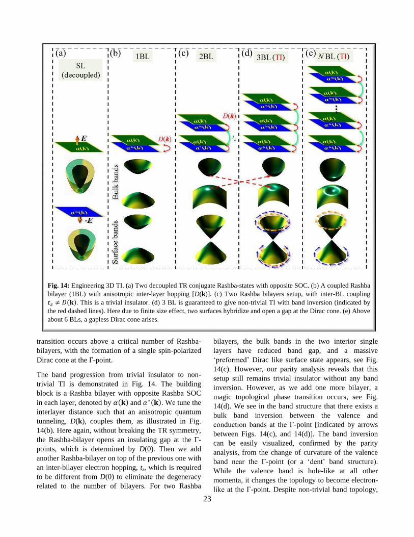
23

transition occurs above a critical number of Rashba-

bilayers, with the formation of a single spin-polarized

Dirac cone at the Γ-point.

The band progression from trivial insulator to non-

trivial TI is demonstrated in Fig. 14. The building

block is a Rashba bilayer with opposite Rashba SOC

in each layer, denoted by 𝛼(𝐤) and 𝛼∗(𝐤). We tune the

interlayer distance such that an anisotropic quantum

tunneling, D(k), couples them, as illustrated in Fig.

14(b). Here again, without breaking the TR symmetry,

the Rashba-bilayer opens an insulating gap at the Г-

points, which is determined by D(0). Then we add

another Rashba-bilayer on top of the previous one with

an inter-bilayer electron hopping, tz, which is required

to be different from D(0) to eliminate the degeneracy

related to the number of bilayers. For two Rashba

bilayers, the bulk bands in the two interior single

layers have reduced band gap, and a massive

‘preformed’ Dirac like surface state appears, see Fig.

14(c). However, our parity analysis reveals that this

setup still remains trivial insulator without any band

inversion. However, as we add one more bilayer, a

magic topological phase transition occurs, see Fig.

14(d). We see in the band structure that there exists a

bulk band inversion between the valence and

conduction bands at the Γ-point [indicated by arrows

between Figs. 14(c), and 14(d)]. The band inversion

can be easily visualized, confirmed by the parity

analysis, from the change of curvature of the valence

band near the Γ-point (or a ‘dent’ band structure).

While the valence band is hole-like at all other

momenta, it changes the topology to become electron-

like at the Γ-point. Despite non-trivial band topology,

Fig. 14: Engineering 3D TI. (a) Two decoupled TR conjugate Rashba-states with opposite SOC. (b) A coupled Rashba

bilayer (1BL) with anisotropic inter-layer hopping [D(k)]. (c) Two Rashba bilayers setup, with inter-BL coupling

𝑡𝑧 ≠ 𝐷(𝐤). This is a trivial insulator. (d) 3 BL is guaranteed to give non-trivial TI with band inversion (indicated by

the red dashed lines). Here due to finite size effect, two surfaces hybridize and open a gap at the Dirac cone. (e) Above

about 6 BLs, a gapless Dirac cone arises.

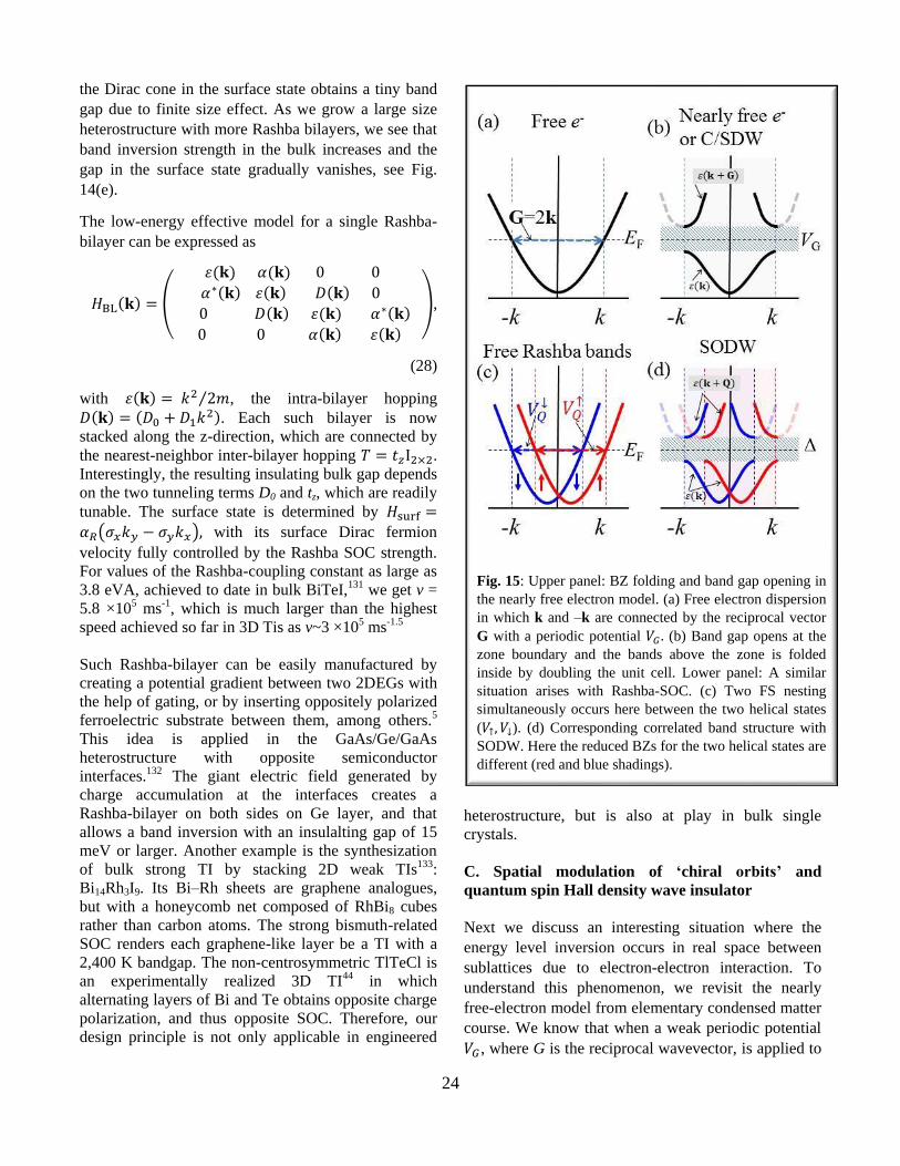
24

the Dirac cone in the surface state obtains a tiny band

gap due to finite size effect. As we grow a large size

heterostructure with more Rashba bilayers, we see that

band inversion strength in the bulk increases and the

gap in the surface state gradually vanishes, see Fig.

14(e).

The low-energy effective model for a single Rashba-

bilayer can be expressed as

𝐻BL(𝐤) = (

휀(𝐤) 𝛼(𝐤) 0 0

𝛼 ∗(𝐤) 휀(𝐤) 𝐷(𝐤) 0

0 𝐷(𝐤) 휀(𝐤) 𝛼 ∗(𝐤)

0 0 𝛼(𝐤) 휀(𝐤)

),

(28)

with 휀(𝐤) = 𝑘2 2𝑚⁄ , the intra-bilayer hopping

𝐷(𝐤) = (𝐷0 + 𝐷1𝑘2). Each such bilayer is now

stacked along the z-direction, which are connected by

the nearest-neighbor inter-bilayer hopping 𝑇 = 𝑡𝑧I2×2.

Interestingly, the resulting insulating bulk gap depends

on the two tunneling terms D0 and tz, which are readily

tunable. The surface state is determined by 𝐻surf =

𝛼𝑅(𝜎𝑥𝑘𝑦 − 𝜎𝑦𝑘𝑥), with its surface Dirac fermion

velocity fully controlled by the Rashba SOC strength.

For values of the Rashba-coupling constant as large as

3.8 eVA, achieved to date in bulk BiTeI,131 we get v =

5.8 ×105 ms-1, which is much larger than the highest

speed achieved so far in 3D Tis as v~3 ×105 ms-1.5

Such Rashba-bilayer can be easily manufactured by

creating a potential gradient between two 2DEGs with

the help of gating, or by inserting oppositely polarized

ferroelectric substrate between them, among others.5

This idea is applied in the GaAs/Ge/GaAs

heterostructure with opposite semiconductor

interfaces.132 The giant electric field generated by

charge accumulation at the interfaces creates a

Rashba-bilayer on both sides on Ge layer, and that

allows a band inversion with an insulalting gap of 15

meV or larger. Another example is the synthesization

of bulk strong TI by stacking 2D weak TIs133:

Bi14Rh3I9. Its Bi–Rh sheets are graphene analogues,

but with a honeycomb net composed of RhBi8 cubes

rather than carbon atoms. The strong bismuth-related

SOC renders each graphene-like layer be a TI with a

2,400 K bandgap. The non-centrosymmetric TlTeCl is

an experimentally realized 3D TI44 in which

alternating layers of Bi and Te obtains opposite charge

polarization, and thus opposite SOC. Therefore, our

design principle is not only applicable in engineered

heterostructure, but is also at play in bulk single

crystals.

C. Spatial modulation of ‘chiral orbits’ and

quantum spin Hall density wave insulator

Next we discuss an interesting situation where the

energy level inversion occurs in real space between

sublattices due to electron-electron interaction. To

understand this phenomenon, we revisit the nearly

free-electron model from elementary condensed matter

course. We know that when a weak periodic potential

𝑉𝐺 , where G is the reciprocal wavevector, is applied to

Fig. 15: Upper panel: BZ folding and band gap opening in

the nearly free electron model. (a) Free electron dispersion

in which k and –k are connected by the reciprocal vector

G with a periodic potential 𝑉𝐺 . (b) Band gap opens at the

zone boundary and the bands above the zone is folded

inside by doubling the unit cell. Lower panel: A similar

situation arises with Rashba-SOC. (c) Two FS nesting

simultaneously occurs here between the two helical states

(𝑉↑,𝑉↓). (d) Corresponding correlated band structure with

SODW. Here the reduced BZs for the two helical states are

different (red and blue shadings).

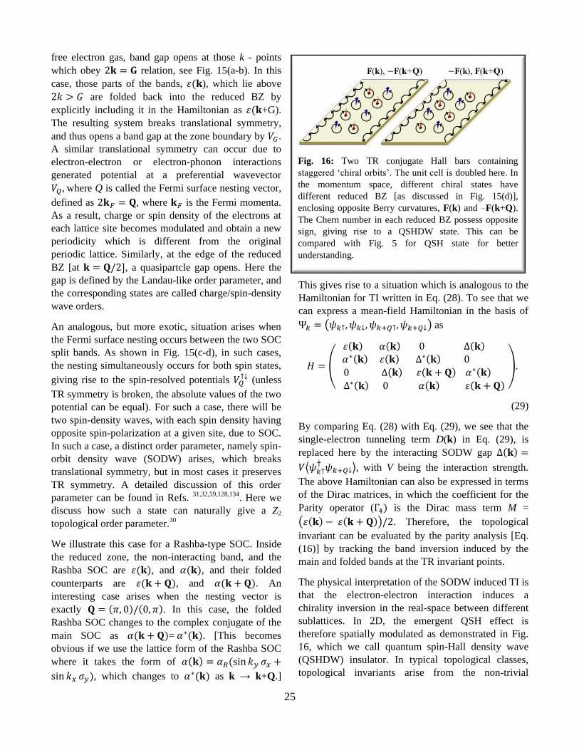
25

free electron gas, band gap opens at those k - points

which obey 2𝐤 = 𝐆 relation, see Fig. 15(a-b). In this

case, those parts of the bands, 휀(𝐤), which lie above

2𝑘 > 𝐺 are folded back into the reduced BZ by

explicitly including it in the Hamiltonian as 휀(𝐤+G).

The resulting system breaks translational symmetry,

and thus opens a band gap at the zone boundary by 𝑉𝐺 .

A similar translational symmetry can occur due to

electron-electron or electron-phonon interactions

generated potential at a preferential wavevector

𝑉𝑄 , where Q is called the Fermi surface nesting vector,

defined as 2𝐤𝐹 = 𝐐, where 𝐤𝐹 is the Fermi momenta.

As a result, charge or spin density of the electrons at

each lattice site becomes modulated and obtain a new

periodicity which is different from the original

periodic lattice. Similarly, at the edge of the reduced

BZ [at 𝐤 = 𝐐/2], a quasipartcle gap opens. Here the

gap is defined by the Landau-like order parameter, and

the corresponding states are called charge/spin-density

wave orders.

An analogous, but more exotic, situation arises when

the Fermi surface nesting occurs between the two SOC

split bands. As shown in Fig. 15(c-d), in such cases,

the nesting simultaneously occurs for both spin states,

giving rise to the spin-resolved potentials 𝑉𝑄↑↓ (unless

TR symmetry is broken, the absolute values of the two

potential can be equal). For such a case, there will be

two spin-density waves, with each spin density having

opposite spin-polarization at a given site, due to SOC.

In such a case, a distinct order parameter, namely spin-

orbit density wave (SODW) arises, which breaks

translational symmetry, but in most cases it preserves

TR symmetry. A detailed discussion of this order

parameter can be found in Refs. 31,32,59,128,134. Here we

discuss how such a state can naturally give a Z2

topological order parameter.30

We illustrate this case for a Rashba-type SOC. Inside

the reduced zone, the non-interacting band, and the

Rashba SOC are 휀(𝐤), and 𝛼(𝐤), and their folded

counterparts are 휀(𝐤 + 𝐐), and 𝛼(𝐤 + 𝐐). An

interesting case arises when the nesting vector is

exactly 𝐐 = (𝜋, 0)/(0, 𝜋). In this case, the folded

Rashba SOC changes to the complex conjugate of the

main SOC as 𝛼(𝐤 + 𝐐)= 𝛼∗(𝐤). [This becomes

obvious if we use the lattice form of the Rashba SOC

where it takes the form of 𝛼(𝐤) = 𝛼𝑅(sin 𝑘𝑦 𝜎𝑥 +

sin 𝑘𝑥 𝜎𝑦), which changes to 𝛼∗(𝐤) as k → k+Q.]

This gives rise to a situation which is analogous to the

Hamiltonian for TI written in Eq. (28). To see that we

can express a mean-field Hamiltonian in the basis of

Ψ𝑘 = (𝜓𝑘↑, 𝜓𝑘↓, 𝜓𝑘+𝑄↑, 𝜓𝑘+𝑄↓) as

𝐻 = (

휀(𝐤) 𝛼(𝐤) 0 ∆(𝐤) 𝛼

∗(𝐤) 휀(𝐤) ∆∗(𝐤) 0

0 ∆(𝐤) 휀(𝐤 + 𝐐) 𝛼 ∗(𝐤)

∆∗(𝐤) 0 𝛼(𝐤) 휀(𝐤 + 𝐐)

).

(29)

By comparing Eq. (28) with Eq. (29), we see that the

single-electron tunneling term D(k) in Eq. (29), is

replaced here by the interacting SODW gap ∆(𝐤) =

𝑉⟨𝜓𝑘↑† 𝜓𝑘+𝑄↓⟩, with V being the interaction strength.

The above Hamiltonian can also be expressed in terms

of the Dirac matrices, in which the coefficient for the

Parity operator (Γ4) is the Dirac mass term M =

(휀(𝐤) − 휀(𝐤 + 𝐐))/2. Therefore, the topological

invariant can be evaluated by the parity analysis [Eq.

(16)] by tracking the band inversion induced by the

main and folded bands at the TR invariant points.

The physical interpretation of the SODW induced TI is

that the electron-electron interaction induces a

chirality inversion in the real-space between different

sublattices. In 2D, the emergent QSH effect is

therefore spatially modulated as demonstrated in Fig.

16, which we call quantum spin-Hall density wave

(QSHDW) insulator. In typical topological classes,

topological invariants arise from the non-trivial

Fig. 16: Two TR conjugate Hall bars containing

staggered ‘chiral orbits’. The unit cell is doubled here. In

the momentum space, different chiral states have

different reduced BZ [as discussed in Fig. 15(d)],

enclosing opposite Berry curvatures, F(k) and –F(k+Q).

The Chern number in each reduced BZ possess opposite

sign, giving rise to a QSHDW state. This can be

compared with Fig. 5 for QSH state for better

understanding.

26

geometry of the band topology of non-interacting

fermions. Electron-electron interaction

does not directly drive a topological phase transition,

except in few cases such as topological Mott, or

Kondo or Anderson insulators, in which, however, no

Landau-type order parameter develops. The proposed

QSHDW phase is a new kind of Landau order

parameter which is associated with topological

invariant. The realization of this order state requires

SOC, strong coulomb interaction, as well as chemical

potential tunability to obtain the desired nesting

wavevector. Quantum wires of Pb, Bi and other SOC

elements are ideal systems to study this problem.128

Because here due to quasi-1D nature, Fermi surface

nesting is enhanced, and here all these three

parameters can be tuned both externally and internally.

The QSHDW phase can also be explored in non-

centrosymmetric heavy-fermion materials which allow

SOC split band structure.

D. Spinless orbital texture inversion induced

topological ‘chiral orbits’

So far we have discussed the formation of magnetic

field free chiral electrons in two methods, namely via

the staggered hopping in SSH model15 or in graphene

lattice,94

and due to SOC. In some of the nodal

superconductors, such as nodal d-wave copper-oxide

superconductors, owing to the particle-hole symmetry,

the quasiparticle dispersion around the discrete nodal

point acts as Dirac excitations.85,86 Therefore, in the

existing classes of Dirac materials, ‘massless’ Dirac

fermions only appears in certain conditions. For

example, Dirac cones only form in atomically thin

layer of graphene, or on the surface states inside the

bulk gap in TI. Therefore, the relevant materials

choices are restricted to heavy elements which, by

nature, have lower band velocity and higher

correlation strength.

Recently, the present author have proposed a new

theory for a distinct type of Dirac materials, called

‘Weyl/Dirac orbital semimetals’ and topological

orbital insulator, which has Weyl/Dirac cone arising

from the orbital texture inversion at discrete momenta

between two orbitals with different symmetries.16,17

The general idea of this design principle lies in

assembling different atoms with distinct conduction

electrons in such a way that the inter-orbital electron

hopping or tunneling term naturally obtains an odd

function of energy-momentum dispersion. Finally, the

intra-orbital terms also conspire in such a way that the

corresponding low-energy Hamiltonian can be reduced

to an effective k.p - type Dirac Hamiltonian. The

resulting Dirac/ Weyl cones at the orbital degenerate

points are protected by lattice/ translational symmetry.

We discuss here a specific example for engineering

Weyl cones. Weyl cones are split Dirac cones arising

from the Dirac Hamiltonian when either inversion or

TR symmetry is lifted, see Fig. 17. We take a layer-by-

layer setup which includes even and odd parity orbitals

in alternating layers - dubbed orbital selective

superlattice. Such structure is odd under mirror

symmetry along the superlattice growth axis. As

shown in Fig. 18, we consider ‘s’ and ‘pz’ orbitals,

placed along the z-direction in different layers, such

that inter-orbital or inter-layer hopping has same

amplitude (unlike in the SSH model15 in which the

amplitude itself is different), but acquires different

sign. The net tunneling matrix-element then becomes

purely imaginary as 휀 𝑠𝑝(𝐤) = −2𝑖𝑡𝑧

𝑠𝑝sin(𝑘𝑧𝑐), where

𝑡𝑧𝑠𝑝

is the hopping amplitude and c is the interlayer

distance. Such complex hopping term can also arise in

various other orbital combinations, such as a

combination of bonding and antibonding states, or

Fig. 17: Bulk Dirac and Weyl cones. (a) A 3D Dirac

cone forming at the TR invariant k-point. Due to the

presence of both TR and inversion (I) symmetry, this

Dirac cone is four-fold degenerate. (b) As inversion

symmetry is lifted, the Dirac cone splits into two Weyl

cones in the momentum directions. Weyl cones must

reside at non-TR k-points otherwise they would

annihilate each other to merge to the 3D Dirac cone

again. (c) Splitting of Dirac cone into Weyl cones along

the energy direction as TR symmetry is lifted. Note that

TR symmetry breaking also leads to splitting of Dirac

cones along the momentum direction.

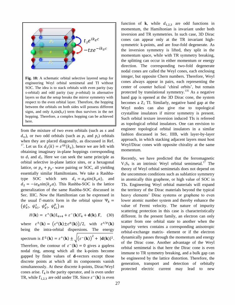
27

from the mixture of two even orbitals (such as s and

dxy), or two odd orbitals (such as px and py) orbitals

when they are placed diagonally, as discussed in Ref. 17. Let us fix 𝑑3(𝑘) = 휀

𝑠𝑝(𝑘𝑧), hence we are left with

obtaining imaginary in-plane hoppings corresponding

to d1 and d2. Here we can seek the same principle as

orbital selective in-plane lattice sites, or a hexagonal

lattice, or 𝑝𝑥 + 𝑝𝑦- wave pairing or SOC, all yielding

essentially similar Hamiltonians. We take a Rashba-

type SOC which sets 𝑑1 = 𝛼𝑅sin(𝑘𝑥𝑎), and

𝑑2 = −𝑖𝛼𝑅sin(𝑘𝑦𝑎). This Rashba-SOC is the lattice

generalization of the same Rashba-SOC discussed in

Sec. IIIC. Now the Hamiltonian can be expressed in

the usual Γ-matrix form in the orbital spinor Ψ𝑘 =

(𝜓𝑘↑𝑠 , 𝜓𝑘↓

𝑠 , 𝜓𝑘↑𝑝

, 𝜓𝑘↓𝑝

) as

𝐻(𝐤) = 휀+(𝐤)𝕀4×4 + 휀−(𝐤)Γ4 + 𝐝(𝐤). 𝚪, (30)

where 휀±(𝐤) = (휀𝑠(𝐤)±휀𝑝(𝐤)) 2⁄ , with 휀𝑠/𝑝(𝐤)

being the intra-orbital dispersions. The energy

spectrum is 𝐸±(𝐤) = 휀+(𝐤) ± √(휀−(𝐤))2

+ |𝐝(𝐤)|2.

Therefore, the contour of 휀−(𝐤) = 0 gives a gapless

nodal ring, among which all the k-points become

gapped by finite values of d-vectors except those

discrete points at which all its components vanish

simultaneously. At these discrete k-points, Dirac/Weyl

cones arise. Γ4 is the parity operator, and is even under

TR, while Γ1,2,3 are odd under TR. Since 휀−(𝐤) is even

function of k, while 𝑑1,2,3 are odd functions in

momentum, the Hamiltonian is invariant under both

inversion and TR symmetries. In such case, 3D Dirac

cones can appear only at the TR invariant high-

symmetric k-points, and are four-fold degenerate. As

the inversion symmetry is lifted, they split in the

momentum space, while with TR symmetry breaking,

the splitting can occur in either momentum or energy

direction. The corresponding two-fold degenerate

nodal cones are called the Weyl cones, each enclosing

integer, but opposite Chern numbers. Therefore, Weyl

cones always appear in pairs, each representing the

center of counter helical ‘chiral orbits’, but remain

protected by translational symmetry.135 As a negative

band gap is opened at the 3D Dirac cone, the system

becomes a Z2 TI. Similarly, negative band gap at the

Weyl nodes can also give rise to topological

crystalline insulators if mirror symmetry is present.

Such orbital texture inversion induced TIs is refereed

as topological orbital insulators. One can envision to

engineer topological orbital insulators in a similar

fashion discussed in Sec. IIIB, with layer-by-layer

approach, in which stacking adjacent layers must host

Weyl/Dirac cones with opposite chirality at the same

momentum.

Recently, we have predicted that the ferromagnetic

V3S4 is an intrinsic Weyl orbital semimetal.17 The

theory of Weyl orbital semimetals does not depend on

the uncommon conditions such as sublattice symmetry

in atomically thin graphene, or high value of SOC in

TIs. Engineering Weyl orbital materials will expand

the territory of the Dirac materials beyond the typical

heavy elements’ Dirac systems or graphene to even

lower atomic number system and thereby enhance the

value of Fermi velocity. The nature of impurity

scattering protection in this case is characteristically

different. In the present family, an electron can only

scatter from one orbital state to another when the

impurity vertex contains a corresponding anisotropic

orbital-exchange matrix- element or if the electron

dynamically passes through the momentum and energy

of the Dirac cone. Another advantage of the Weyl

orbital semimetal is that here the Dirac cone is even

immune to TR symmetry breaking, and a bulk gap can

be engineered by the lattice distortion. Therefore, the

generation, transport and detection of orbitally

protected electric current may lead to new

Fig. 18: A schematic orbital selective layered setup for

engineering Weyl orbital semimetal and TI without

SOC. The idea is to stack orbitals with even parity (say

s-orbital) and odd parity (say p-orbital) in alternative

layers so that the setup breaks the mirror symmetry with

respect to the even orbital layer. Therefore, the hopping

between the orbitals on both sides will possess different

signs, and only itzsin(kzc) term thus survives in the net

hopping. Therefore, a complex hopping can be achieved

here.

28

opportunities for orbitronics. Chiral orbital current in

the Weyl semimetals can be detected by Kerr effect.

IV. Conclusion and outlook This article presented a thorough understanding of the

topological invariants in the absence and presence of

TR symmetry, as well as other symmetries such as

inversion symmetry, mirror symmetry, or particle-hole

symmetry. The historical development of the

topological invariant starting from the quantization of

flux through a non-trivial Gaussian curvature to the

IQH to QSH to Z2 TI provides a more transparent and

step-by-step development of this field. A unique

feature of this field is that it blends concepts from

various fields including mathematics, condensed

matter physics, chemistry, and particle physics. A

detailed discussion of the materials chemistry of the TI

systems is left out in this article and can be found

elsewhere.63 We can highlight an interesting difference

between the trivial insulator and TI from a chemist’s

perspective. In a band insulator, the valence and

conduction bands remain fully filled and empty,

respectively. Therefore, such insulators are sought in

elements or compounds whose outer most orbital

contains even number of electrons. TI is also a ‘band

insulator’ with a twist. Here the valence and

conduction bands are also expected to be completely

filled and empty, respectively, but at the same time,

these bands are inverted at the TR invariant k-points,

suggesting otherwise. Therefore, one can neither seek

for elements with completely full outermost orbital,

nor partially filled orbital (since partially filled state

should give a metallic state). For the same reason, the

material should neither be too covalent, nor too ionic.

Therefore intermetallics are obvious elements to

consider for non-interacting TI (interaction can change

this simple explanation). Indeed, most of the TIs are

made of intermetallics. Here we can consider at least

two partially occupied elements which participate in

orbital-overlap and/or coupled via SOC. Therefore, a

band can remained fully occupied by accommodating

two partially filled orbitals. If the exchange of the

orbital character occurs at odd number of TR invariant

points, it gives rise to ‘strong’ TI, otherwise even

number of orbital weight switching can give rise to

either a ‘weak’ TI or a trivial insulator.

From high-energy physicists’ perspective, TI field

offers a plenty of new opportunities to predict new

excitations as well as to realize some of the uncharted

‘particles’ predicted there. Weyl fermions136–139 and

Majorana fermions140–142 which remained elusive for

decades have only been realized recently in TI

platforms. Axion,24,104 and anyons143,144 are two widely

searched excitations which are predicted to be present

in TIs. Recently, it is shown that supersymmetry

(SUSY) can be found in TI and superconductor

heterostructures.145,146

Cold atom physicists also find it interesting to

contribute to the TI fields in various ways. Haldane, in

his original paper,3 commented that “the particular

model presented here is unlikely to be directly

physically realizable”. Cold atom researchers have

made it possible to create the Haldane model with

optically generated honeycomb lattice.96 They have

engineered TR and inversion symmetry breakings by

carefully enhancing next-nearest-neighbor hopping

and providing staggered onsite energies to different

sublattices, respectively, as proposed by Haldane.

More recently, protected edge state is generated in

various optical lattice structure by employing synthetic

gauge field.147,148 The apparent setback to realize the

Z2 TI due to the lack of 2D SOC can be overcame with

our engineered structure (as discussed in Sec. IIIA),79

and the realization of TR invariant TI in optical lattice

field is a matter of time. Due to tremendous controls

over structural and quantum properties in these setups,

an unprecedented tunability of TI properties for further

exploration can be possible here.

Despite the predictions and discoveries of several TI

materials classes, materials flexibility still remains a

grand challenge.63 Bi2Se3 family is widely used for

many experiments on TI since both single crystal, and

thin films of this system can be easily grown.

HgTe/CdTe33 and InAs/GaSb72 are the only two

systems experimentally demonstrated as QSH

insulators, which are however not being used in other

experiments. Magnetic doped thin film of Bi2Se3 is the

only system synthesized so far to be QAH

insulator.107,108 Pb1-xSnxSe/Te52–54 and SnS55 are the

only two systems known to be topological crystalline

insulator. SmB6 is predicted and subsequently realized

to be topological Kondo insulator,56,149,150 although

evidence against this conclusion is also present.151

Cd3As2,152,153 and Na3Bi154,155 are synthesized to be 3D

TI, while TaAs,136–138 and NbAs139 family is discerned

recently to be Weyl semimetal. Many other families,

such as topological Mott insulator, topological

Anderson insulator, and topological axion insulators

are yet to be discovered. Moreover, the inevitable

29

presence of the bulk conductivity in most of the 3D TI

samples poses a serious nuisance to experimentalists.

On the other hand, engineering TI can be rather

simpler. It also offers tremendous versatility in terms

of materials growth, and obtaining quantum and

topological properties. Therefore, the successful

preparation of ‘home-made’ TI will caters to many

physicists, chemists and engineers seeking suitable

materials with higher tunability and materials

flexibility.

Acknowledgments

I have many people to thank for their generous

collaborations, discussions, and lessions on various

aspects of topological states of matter and other related

concepts which led to the completion of this article.

There is a possibility that I fail to acknowledge

everybody here to the rush in finishing this article. The

people I can immediately recall to convey my

gratitude are: Arun Bansil, Alexander Balatsky, Hsin

Lin, Le-Quy Duong, F.-C. Chuang, M. Zahid Hasan,

Diptiman Sen, Anindya Das, Aveek Bid, Tirupathaiah

Setti, Vidya Madhavan, Robert Markiewicz, Matthias

Graf, Jian-Xin Zhou, Christoph Tegenkamp, J. Hugo

Dil. Kapildeb Dolui, Gaurav Gupta, Sujay Ray,

Ananya Ghatak, Sayonee Ray, Kallol Sen, Soumi

Ghosh, Kausik Ghosh.

References 1 R.B. Laughlin, Phys. Rev. B 23, 5632 (1981). 2 D.J. Thouless, M. Kohmoto, M.P. Nightingale, and

M. den Nijs, Phys. Rev. Lett. 49, 405 (1982). 3 F.D.M. Haldane, Phys. Rev. Lett. 61, 2015 (1988). 4 C.L. Kane and E.J. Mele, Phys. Rev. Lett. 95,

226801 (2005). 5 T. Das and A.V. Balatsky, Nat. Commun. 4, 1972

(2013). 6 L. Fu, C.L. Kane, and E.J. Mele, Phys. Rev. Lett. 98,

106803 (2007). 7 L. Fu and C.L. Kane, Phys. Rev. B 76, 045302

(2007). 8 J.C.Y. Teo, L. Fu, and C.L. Kane, Phys. Rev. B 78,

045426 (2008). 9 B.A. Bernevig, T.L. Hughes, and S.-C. Zhang,

Science 314, 1757 (2006). 10 T. Fukui and Y. Hatsugai, J. Phys. Soc. Jpn. 76,

053702 (2007). 11 J.E. Moore and L. Balents, Phys. Rev. B 75, 121306

(2007).

12 R. Roy, Phys. Rev. B 79, 195322 (2009). 13 T. Fukui, T. Fujiwara, and Y. Hatsugai, J. Phys. Soc.

Jpn. 77, 123705 (2008). 14 X.-L. Qi, T.L. Hughes, and S.-C. Zhang, Phys. Rev.

B 78, 195424 (2008). 15 W.P. Su, J.R. Schrieffer, and A.J. Heeger, Phys.

Rev. B 22, 2099 (1980). 16 T. Das, Phys. Rev. B 88, 035444 (2013). 17 K. Dolui and T. Das, ArXiv14122607 Cond-Mat

(2014). 18 H. Zhang, C.-X. Liu, X.-L. Qi, X. Dai, Z. Fang, and

S.-C. Zhang, Nat. Phys. 5, 438 (2009). 19 Y. Xia, D. Qian, D. Hsieh, L. Wray, A. Pal, H. Lin,

A. Bansil, D. Grauer, Y.S. Hor, R.J. Cava, and M.Z.

Hasan, Nat. Phys. 5, 398 (2009). 20 H. Lin, T. Das, Y.J. Wang, L.A. Wray, S.-Y. Xu,

M.Z. Hasan, and A. Bansil, Phys. Rev. B 87, 121202

(2013). 21 L. Fu, Phys. Rev. Lett. 106, 106802 (2011). 22 X.-L. Qi, T.L. Hughes, S. Raghu, and S.-C. Zhang,

Phys. Rev. Lett. 102, 187001 (2009). 23 X.-L. Qi and S.-C. Zhang, Rev. Mod. Phys. 83, 1057

(2011). 24 A.M. Essin, J.E. Moore, and D. Vanderbilt, Phys.

Rev. Lett. 102, 146805 (2009). 25 X. Wan, A. Vishwanath, and S.Y. Savrasov, Phys.

Rev. Lett. 108, 146601 (2012). 26 C.W. Groth, M. Wimmer, A.R. Akhmerov, J.

Tworzydło, and C.W.J. Beenakker, Phys. Rev. Lett.

103, 196805 (2009). 27 J. Li, R.-L. Chu, J.K. Jain, and S.-Q. Shen, Phys.

Rev. Lett. 102, 136806 (2009). 28 M. Dzero, K. Sun, V. Galitski, and P. Coleman,

Phys. Rev. Lett. 104, 106408 (2010). 29 S. Raghu, X.-L. Qi, C. Honerkamp, and S.-C.

Zhang, Phys. Rev. Lett. 100, 156401 (2008). 30 G. Gupta and T. Das, Manuscr. Prep. (n.d.). 31 T. Das, Sci. Rep. 2, (2012). 32 T. Das, Phys. Rev. Lett. 109, 246406 (2012). 33 M. König, S. Wiedmann, C. Brüne, A. Roth, H.

Buhmann, L.W. Molenkamp, X.-L. Qi, and S.-C.

Zhang, Science 318, 766 (2007). 34 D. Hsieh, D. Qian, L. Wray, Y. Xia, Y.S. Hor, R.J.

Cava, and M.Z. Hasan, Nature 452, 970 (2008). 35 Y.L. Chen, J.G. Analytis, J.-H. Chu, Z.K. Liu, S.-K.

Mo, X.L. Qi, H.J. Zhang, D.H. Lu, X. Dai, Z. Fang,

S.C. Zhang, I.R. Fisher, Z. Hussain, and Z.-X. Shen,

Science 325, 178 (2009). 36 S.-Y. Xu, L.A. Wray, Y. Xia, R. Shankar, A.

Petersen, A. Fedorov, H. Lin, A. Bansil, Y.S. Hor, D.

Grauer, R.J. Cava, and M.Z. Hasan, ArXiv10075111

Cond-Mat Physicsphysics Physicsquant-Ph (2010).

30

37 H. Lin, L.A. Wray, Y. Xia, S. Xu, S. Jia, R.J. Cava,

A. Bansil, and M.Z. Hasan, Nat. Mater. 9, 546 (2010). 38 S. Chadov, X. Qi, J. Kübler, G.H. Fecher, C. Felser,

and S.C. Zhang, Nat. Mater. 9, 541 (2010). 39 H. Lin, R.S. Markiewicz, L.A. Wray, L. Fu, M.Z.

Hasan, and A. Bansil, Phys. Rev. Lett. 105, 036404

(2010). 40 B. Yan, C.-X. Liu, H.-J. Zhang, C.-Y. Yam, X.-L.

Qi, T. Frauenheim, and S.-C. Zhang, EPL Europhys.

Lett. 90, 37002 (2010). 41 Y.J. Wang, H. Lin, T. Das, M.Z. Hasan, and A.

Bansil, New J. Phys. 13, 085017 (2011). 42 H.-J. Zhang, S. Chadov, L. Müchler, B. Yan, X.-L.

Qi, J. Kübler, S.-C. Zhang, and C. Felser, Phys. Rev.

Lett. 106, 156402 (2011). 43 S. Lee, J. In, Y. Yoo, Y. Jo, Y.C. Park, H. Kim, H.C.

Koo, J. Kim, B. Kim, and K.L. Wang, Nano Lett. 12,

4194 (2012). 44 Y.L. Chen, M. Kanou, Z.K. Liu, H.J. Zhang, J.A.

Sobota, D. Leuenberger, S.K. Mo, B. Zhou, S.-L.

Yang, P.S. Kirchmann, D.H. Lu, R.G. Moore, Z.

Hussain, Z.X. Shen, X.L. Qi, and T. Sasagawa, Nat.

Phys. 9, 704 (2013). 45 G. Landolt, S.V. Eremeev, O.E. Tereshchenko, S.

Muff, B. Slomski, K.A. Kokh, M. Kobayashi, T.

Schmitt, V.N. Strocov, J. Osterwalder, E.V. Chulkov,

and J.H. Dil, New J. Phys. 15, 085022 (2013). 46 M.S. Bahramy, B.-J. Yang, R. Arita, and N.

Nagaosa, Nat. Commun. 3, 679 (2012). 47 Y. Xu, B. Yan, H.-J. Zhang, J. Wang, G. Xu, P.

Tang, W. Duan, and S.-C. Zhang, Phys. Rev. Lett.

111, 136804 (2013). 48 Y. Wang, W. Ji, C. Zhang, P. Li, F. Li, M. Ren, X.-

L. Chen, M. Yuan, and P. Wang, Sci. Rep. 6, 20342

(2016). 49 F.-C. Chuang, L.-Z. Yao, Z.-Q. Huang, Y.-T. Liu,

C.-H. Hsu, T. Das, H. Lin, and A. Bansil, Nano Lett.

14, 2505 (2014). 50 Y. Lu, W. Xu, M. Zeng, G. Yao, L. Shen, M. Yang,

Z. Luo, F. Pan, K. Wu, T. Das, P. He, J. Jiang, J.

Martin, Y.P. Feng, H. Lin, and X. Wang, Nano Lett.

15, 80 (2015). 51 Q. Liu, X. Zhang, L.B. Abdalla, A. Fazzio, and A.

Zunger, Nano Lett. 15, 1222 (2015). 52 P. Dziawa, B.J. Kowalski, K. Dybko, R. Buczko, A.

Szczerbakow, M. Szot, E. Łusakowska, T.

Balasubramanian, B.M. Wojek, M.H. Berntsen, O.

Tjernberg, and T. Story, Nat. Mater. 11, 1023 (2012). 53 T.H. Hsieh, H. Lin, J. Liu, W. Duan, A. Bansil, and

L. Fu, Nat. Commun. 3, 982 (2012). 54 Y. Okada, M. Serbyn, H. Lin, D. Walkup, W. Zhou,

C. Dhital, M. Neupane, S. Xu, Y.J. Wang, R. Sankar,

F. Chou, A. Bansil, M.Z. Hasan, S.D. Wilson, L. Fu,

and V. Madhavan, Science 341, 1496 (2013). 55 Y. Sun, Z. Zhong, T. Shirakawa, C. Franchini, D. Li,

Y. Li, S. Yunoki, and X.-Q. Chen, Phys. Rev. B 88,

235122 (2013). 56 J.D. Denlinger, J.W. Allen, J.-S. Kang, K. Sun, B.-I.

Min, D.-J. Kim, and Z. Fisk, (2013). 57 T.-R. Chang, T. Das, P.-J. Chen, M. Neupane, S.-Y.

Xu, M.Z. Hasan, H. Lin, H.-T. Jeng, and A. Bansil,

Phys. Rev. B 91, 155151 (2015). 58 X. Zhang, H. Zhang, J. Wang, C. Felser, and S.-C.

Zhang, Science 335, 1464 (2012). 59 T. Das, Phys. Rev. B 89, 045135 (2014). 60 T. Das, Philos. Mag. 94, 3838 (2014). 61 C.-X. Liu, S.-C. Zhang, and X.-L. Qi,

ArXiv150807106 Cond-Mat (2015). 62 K. Dolui, S. Ray, and T. Das, Phys. Rev. B 92,

205133 (2015). 63 A. Bansil, H. Lin, and T. Das, ArXiv160303576

Cond-Mat Rev. Mod. Phys. (2015). 64 Y. Ando, J. Phys. Soc. Jpn. 82, 102001 (2013). 65 S.-Y. Xu, Y. Xia, L.A. Wray, S. Jia, F. Meier, J.H.

Dil, J. Osterwalder, B. Slomski, A. Bansil, H. Lin, R.J.

Cava, and M.Z. Hasan, Science 332, 560 (2011). 66 M. Koleini, T. Frauenheim, and B. Yan, Phys. Rev.

Lett. 110, 016403 (2013). 67 I. Efthimiopoulos, J. Kemichick, X. Zhou, S.V.

Khare, D. Ikuta, and Y. Wang, J. Phys. Chem. A 118,

1713 (2014). 68 J.J. Hamlin, J.R. Jeffries, N.P. Butch, P. Syers, D.A.

Zocco, S.T. Weir, Y.K. Vohra, J. Paglione, and M.B.

Maple, J. Phys.-Condens. Matter 24, 035602 (2012). 69 L. Wu, M. Brahlek, R. Valdés Aguilar, A.V. Stier,

C.M. Morris, Y. Lubashevsky, L.S. Bilbro, N. Bansal,

S. Oh, and N.P. Armitage, Nat. Phys. 9, 410 (2013). 70 T.V. Menshchikova, M.M. Otrokov, S.S. Tsirkin,

D.A. Samorokov, V.V. Bebneva, A. Ernst, V.M.

Kuznetsov, and E.V. Chulkov, Nano Lett. 13, 6064

(2013). 71 G. Wu, H. Chen, Y. Sun, X. Li, P. Cui, C. Franchini,

J. Wang, X.-Q. Chen, and Z. Zhang, Sci. Rep. 3,

(2013). 72 I. Knez, R.-R. Du, and G. Sullivan, Phys. Rev. Lett.

107, 136603 (2011). 73 C. Weeks, J. Hu, J. Alicea, M. Franz, and R. Wu,

Phys. Rev. X 1, 021001 (2011). 74 A. Kormányos, V. Zólyomi, N.D. Drummond, and

G. Burkard, Phys. Rev. X 4, 011034 (2014). 75 A. Avsar, J.Y. Tan, T. Taychatanapat, J.

Balakrishnan, G.K.W. Koon, Y. Yeo, J. Lahiri, A.

Carvalho, A.S. Rodin, E.C.T. O’Farrell, G. Eda, A.H.

Castro Neto, and B. Özyilmaz, Nat. Commun. 5, 4875

(2014).

31

76 D. Xiao, W. Zhu, Y. Ran, N. Nagaosa, and S.

Okamoto, Nat. Commun. 2, 596 (2011). 77 B. Wunsch, F. Guinea, and F. Sols, New J. Phys. 10,

103027 (2008). 78 B. Dóra, J. Cayssol, F. Simon, and R. Moessner,

Phys. Rev. Lett. 108, 056602 (2012). 79 S. Ray, K. Sen, and T. Das, ArXiv160202926 Cond-

Mat (2016). 80 M.Z. Hasan and C.L. Kane, Rev. Mod. Phys. 82,

3045 (2010). 81 H. Zhang and S.-C. Zhang, Phys. Status Solidi RRL

– Rapid Res. Lett. 7, 72 (2013). 82 S.R. Elliott and M. Franz, ArXiv14034976 Cond-

Mat Physicshep-Ex Physicsnucl-Ex (2014). 83 C.W.J. Beenakker, Annu. Rev. Condens. Matter

Phys. 4, 113 (2013). 84 J. Maciejko, T.L. Hughes, and S.-C. Zhang, Annu.

Rev. Condens. Matter Phys. 2, 31 (2011). 85 T.O. Wehling, A.M. Black-Schaffer, and A.V.

Balatsky, Adv. Phys. 63, 1 (2014). 86 O. Vafek and A. Vishwanath, Annu. Rev. Condens.

Matter Phys. 5, 83 (2014). 87 S.-Q. Shen, Topological Insulators (Springer Berlin

Heidelberg, Berlin, Heidelberg, 2012). 88 B.A. Bernevig and T.L. Hughes, Topological

Insulators and Topological Superconductors

(Princeton University Press, 2013). 89 T. Yoshida, S. Fujimoto, and N. Kawakami, Phys.

Rev. B 85, 125113 (2012). 90 Z. Wang and S.-C. Zhang, Phys. Rev. X 2, 031008

(2012). 91 K. v. Klitzing, G. Dorda, and M. Pepper, Phys. Rev.

Lett. 45, 494 (1980). 92 Q. Niu, D.J. Thouless, and Y.-S. Wu, Phys. Rev. B

31, 3372 (1985). 93 M.V. Berry, Proc. R. Soc. Lond. Math. Phys. Sci.

392, 45 (1984). 94 A.H. Castro Neto, F. Guinea, N.M.R. Peres, K.S.

Novoselov, and A.K. Geim, Rev. Mod. Phys. 81, 109

(2009). 95 J. Zak, Phys. Rev. Lett. 62, 2747 (1989). 96 G. Jotzu, M. Messer, R. Desbuquois, M. Lebrat, T.

Uehlinger, D. Greif, and T. Esslinger, Nature 515, 237

(2014). 97 L. Fu and C.L. Kane, Phys. Rev. B 74, 195312

(2006). 98 A.A. Soluyanov and D. Vanderbilt, Phys. Rev. B 83,

035108 (2011). 99 Z. Ringel and Y.E. Kraus, Phys. Rev. B 83, 245115

(2011). 100 R. Yu, X.L. Qi, A. Bernevig, Z. Fang, and X. Dai,

Phys. Rev. B 84, 075119 (2011). 101 F. Wilczek, Phys. Rev. Lett. 58, 1799 (1987).

102 S.C. Zhang, T.H. Hansson, and S. Kivelson, Phys.

Rev. Lett. 62, 82 (1989). 103 X.G. Wen and Q. Niu, Phys. Rev. B 41, 9377

(1990). 104 R. Li, J. Wang, X.-L. Qi, and S.-C. Zhang, Nat.

Phys. 6, 284 (2010). 105 A. Sekine and K. Nomura, J. Phys. Soc. Jpn. 83,

104709 (2014). 106 J. Wang, R. Li, S.-C. Zhang, and X.-L. Qi, Phys.

Rev. Lett. 106, 126403 (2011). 107 C.-Z. Chang, J. Zhang, X. Feng, J. Shen, Z. Zhang,

M. Guo, K. Li, Y. Ou, P. Wei, L.-L. Wang, Z.-Q. Ji,

Y. Feng, S. Ji, X. Chen, J. Jia, X. Dai, Z. Fang, S.-C.

Zhang, K. He, Y. Wang, L. Lu, X.-C. Ma, and Q.-K.

Xue, Science 340, 167 (2013). 108 C.-Z. Chang, W. Zhao, D.Y. Kim, H. Zhang, B.A.

Assaf, D. Heiman, S.-C. Zhang, C. Liu, M.H.W. Chan,

and J.S. Moodera, Nat. Mater. 14, 473 (2015). 109 L.Q. Duong, T. Das, Y.P. Feng, and H. Lin, J.

Appl. Phys. 117, 17C741 (2015). 110 P. Streda, J. Phys. C Solid State Phys. 15, L1299

(1982). 111 Z. Wang, X.-L. Qi, and S.-C. Zhang, Phys. Rev.

Lett. 105, 256803 (2010). 112 T. Das, R.S. Markiewicz, and A. Bansil, Adv. Phys.

63, 151 (2014). 113 T. Das, J.-X. Zhu, and M.J. Graf, Phys. Rev. Lett.

108, 017001 (2012). 114 T. Das and K. Dolui, Phys. Rev. B 91, 094510

(2015). 115 R.S. Dhaka, T. Das, N.C. Plumb, Z. Ristic, W.

Kong, C.E. Matt, N. Xu, K. Dolui, E. Razzoli, M.

Medarde, L. Patthey, M. Shi, M. Radović, and J.

Mesot, Phys. Rev. B 92, 035127 (2015). 116 T. Das, T. Durakiewicz, J.-X. Zhu, J.J. Joyce, J.L.

Sarrao, and M.J. Graf, Phys. Rev. X 2, 041012 (2012). 117 S. Basak, T. Das, H. Lin, J. Nieminen, M. Lindroos,

R.S. Markiewicz, and A. Bansil, Phys. Rev. B 80,

214520 (2009). 118 R. Roy and C. Kallin, Phys. Rev. B 77, 174513

(2008). 119 A. Kitaev, in AIP Conf. Proc. (AIP Publishing,

2009), pp. 22–30. 120 A.P. Schnyder, S. Ryu, A. Furusaki, and A.W.W.

Ludwig, Phys. Rev. B 78, 195125 (2008). 121 N. Read and D. Green, Phys. Rev. B 61, 10267

(2000). 122 D.A. Ivanov, Phys. Rev. Lett. 86, 268 (2001). 123 L. Fu and C.L. Kane, Phys. Rev. Lett. 100, 096407

(2008). 124 N. Aharon, M. Drewsen, and A. Retzker, Phys.

Rev. Lett. 111, 230507 (2013).

32

125 H. Lin, T. Das, Y. Okada, M.C. Boyer, W.D. Wise,

M. Tomasik, B. Zhen, E.W. Hudson, W. Zhou, V.

Madhavan, C.-Y. Ren, H. Ikuta, and A. Bansil, Nano

Lett. 13, 1915 (2013). 126 H. Lin, T. Das, L.A. Wray, S.-Y. Xu, M.Z. Hasan,

and A. Bansil, New J. Phys. 13, 095005 (2011). 127 N. Goldman, F. Gerbier, and M. Lewenstein, J.

Phys. B-At. Mol. Opt. Phys. 46, 134010 (2013). 128 C. Brand, H. Pfnür, G. Landolt, S. Muff, J.H. Dil,

T. Das, and C. Tegenkamp, Nat. Commun. 6, 8118

(2015). 129 Y.-J. Lin, K. Jiménez-García, and I.B. Spielman,

Nature 471, 83 (2011). 130 V. Galitski and I.B. Spielman, Nature 494, 49

(2013). 131 K. Ishizaka, M.S. Bahramy, H. Murakawa, M.

Sakano, T. Shimojima, T. Sonobe, K. Koizumi, S.

Shin, H. Miyahara, A. Kimura, K. Miyamoto, T.

Okuda, H. Namatame, M. Taniguchi, R. Arita, N.

Nagaosa, K. Kobayashi, Y. Murakami, R. Kumai, Y.

Kaneko, Y. Onose, and Y. Tokura, Nat. Mater. 10, 521

(2011). 132 D. Zhang, W. Lou, M. Miao, S. Zhang, and K.

Chang, Phys. Rev. Lett. 111, 156402 (2013). 133 B. Rasche, A. Isaeva, M. Ruck, S. Borisenko, V.

Zabolotnyy, B. Büchner, K. Koepernik, C. Ortix, M.

Richter, and J. van den Brink, Nat. Mater. 12, 422

(2013). 134 T. Das, J. Supercond. Nov. Magn. 26, 1673 (2012). 135 Z. Huang, T. Das, A.V. Balatsky, and D.P. Arovas,

Phys. Rev. B 87, 155123 (2013). 136 B.Q. Lv, N. Xu, H.M. Weng, J.Z. Ma, P. Richard,

X.C. Huang, L.X. Zhao, G.F. Chen, C.E. Matt, F.

Bisti, V.N. Strocov, J. Mesot, Z. Fang, X. Dai, T.

Qian, M. Shi, and H. Ding, Nat. Phys. 11, 724 (2015). 137 L.X. Yang, Z.K. Liu, Y. Sun, H. Peng, H.F. Yang,

T. Zhang, B. Zhou, Y. Zhang, Y.F. Guo, M. Rahn, D.

Prabhakaran, Z. Hussain, S.-K. Mo, C. Felser, B. Yan,

and Y.L. Chen, Nat. Phys. 11, 728 (2015). 138 S.-Y. Xu, I. Belopolski, N. Alidoust, M. Neupane,

G. Bian, C. Zhang, R. Sankar, G. Chang, Z. Yuan, C.-

C. Lee, S.-M. Huang, H. Zheng, J. Ma, D.S. Sanchez,

B. Wang, A. Bansil, F. Chou, P.P. Shibayev, H. Lin, S.

Jia, and M.Z. Hasan, Science 349, 613 (2015). 139 S.-Y. Xu, N. Alidoust, I. Belopolski, Z. Yuan, G.

Bian, T.-R. Chang, H. Zheng, V.N. Strocov, D.S.

Sanchez, G. Chang, C. Zhang, D. Mou, Y. Wu, L.

Huang, C.-C. Lee, S.-M. Huang, B. Wang, A. Bansil,

H.-T. Jeng, T. Neupert, A. Kaminski, H. Lin, S. Jia,

and M. Zahid Hasan, Nat. Phys. 11, 748 (2015). 140 V. Mourik, K. Zuo, S.M. Frolov, S.R. Plissard, E.P.

a. M. Bakkers, and L.P. Kouwenhoven, Science 336,

1003 (2012).

141 A. Das, Y. Ronen, Y. Most, Y. Oreg, M. Heiblum,

and H. Shtrikman, Nat. Phys. 8, 887 (2012). 142 S. Nadj-Perge, I.K. Drozdov, J. Li, H. Chen, S.

Jeon, J. Seo, A.H. MacDonald, B.A. Bernevig, and A.

Yazdani, Science 346, 602 (2014). 143 A.Y. Kitaev, Ann. Phys. 303, 2 (2003). 144 A. Rahmani, R.A. Muniz, and I. Martin, Phys. Rev.

X 3, 031008 (2013). 145 T. Grover, D.N. Sheng, and A. Vishwanath,

Science 344, 280 (2014). 146 A. Rahmani, X. Zhu, M. Franz, and I. Affleck,

Phys. Rev. Lett. 115, 166401 (2015). 147 M. Mancini, G. Pagano, G. Cappellini, L. Livi, M.

Rider, J. Catani, C. Sias, P. Zoller, M. Inguscio, M.

Dalmonte, and L. Fallani, Science 349, 1510 (2015). 148 B.K. Stuhl, H.-I. Lu, L.M. Aycock, D. Genkina,

and I.B. Spielman, Science 349, 1514 (2015). 149 J. Jiang, S. Li, T. Zhang, Z. Sun, F. Chen, Z.R. Ye,

M. Xu, Q.Q. Ge, S.Y. Tan, X.H. Niu, M. Xia, B.P.

Xie, Y.F. Li, X.H. Chen, H.H. Wen, and D.L. Feng,

Nat. Commun. 4, 3010 (2013). 150 M. Neupane, N. Alidoust, S.-Y. Xu, T. Kondo, Y.

Ishida, D.J. Kim, C. Liu, I. Belopolski, Y.J. Jo, T.-R.

Chang, H.-T. Jeng, T. Durakiewicz, L. Balicas, H. Lin,

A. Bansil, S. Shin, Z. Fisk, and M.Z. Hasan, Nat.

Commun. 4, 2991 (2013). 151 Z.-H. Zhu, A. Nicolaou, G. Levy, N.P. Butch, P.

Syers, X.F. Wang, J. Paglione, G.A. Sawatzky, I.S.

Elfimov, and A. Damascelli, Phys. Rev. Lett. 111,

216402 (2013). 152 S. Borisenko, Q. Gibson, D. Evtushinsky, V.

Zabolotnyy, B. Büchner, and R.J. Cava, Phys. Rev.

Lett. 113, 027603 (2014). 153 M. Neupane, S.-Y. Xu, R. Sankar, N. Alidoust, G.

Bian, C. Liu, I. Belopolski, T.-R. Chang, H.-T. Jeng,

H. Lin, A. Bansil, F. Chou, and M.Z. Hasan, Nat.

Commun. 5, 3786 (2014). 154 Z. Wang, Y. Sun, X.-Q. Chen, C. Franchini, G. Xu,

H. Weng, X. Dai, and Z. Fang, Phys. Rev. B 85,

195320 (2012). 155 Z.K. Liu, B. Zhou, Y. Zhang, Z.J. Wang, H.M.

Weng, D. Prabhakaran, S.-K. Mo, Z.X. Shen, Z. Fang,

X. Dai, Z. Hussain, and Y.L. Chen, Science 343, 864

(2014).