International Journal of Advanced Robotic Systems

A Path Tracking Algorithm Using Future Prediction Control with Spike Detection for an Autonomous Vehicle Robot Regular Paper

Muhammad Aizzat Zakaria1, Hairi Zamzuri1,*, Rosbi Mamat2 and Saiful Amri Mazlan3 1 UTM-PROTON Active Safety Laboratory, Universiti Teknologi, Malaysia 2 Department of Control and Mechatronic Engineering, Faculty of Electrical Engineering, Universiti Teknologi Malaysia 3 Vehicle System Engineering Research Laboratory, Malaysia-Japan International Institute of Technology, Universiti Teknologi, Malaysia * Corresponding author E-mail: hairi@ic.utm.my Received 18 Dec 2012; Accepted 20 May 2013 DOI: 10.5772/56658 © 2013 Zakaria et al.; licensee InTech. This is an open access article distributed under the terms of the Creative Commons Attribution License (http://creativecommons.org/licenses/by/3.0), which permits unrestricted use, distribution, and reproduction in any medium, provided the original work is properly cited.

Abstract Trajectory tracking is an important aspect of autonomous vehicles. The idea behind trajectory tracking is the ability of the vehicle to follow a predefined path with zero steady state error. The difficulty arises due to the nonlinearity of vehicle dynamics. Therefore, this paper proposes a stable tracking control for an autonomous vehicle. An approach that consists of steering wheel control and lateral control is introduced. This control algorithm is used for a non-holonomic navigation problem, namely tracking a reference trajectory in a closed loop form. A proposed future prediction point control algorithm is used to calculate the vehicle’s lateral error in order to improve the performance of the trajectory tracking. A feedback sensor signal from the steering wheel angle and yaw rate sensor is used as feedback information for the controller. The controller consists of a relationship between the future point lateral error, the linear velocity, the heading error and the reference yaw rate. This paper also introduces a spike detection algorithm to track the spike error that occurs during GPS reading. The proposed idea is to take the advantage of the derivative of the steering rate. This

paper aims to tackle the lateral error problem by applying the steering control law to the vehicle, and proposes a new path tracking control method by considering the future coordinate of the vehicle and the future estimated lateral error. The effectiveness of the proposed controller is demonstrated by a simulation and a GPS experiment with noisy data. The approach used in this paper is not limited to autonomous vehicles alone since the concept of autonomous vehicle tracking can be used in mobile robot platforms, as the kinematic model of these two platforms is similar. Keywords Trajectory Tracking, Mobile Robot, Autonomous Vehicle, Yaw Rate Control, Path Following, Steering Control, Spike Control

1. Introduction Autonomous vehicles are a rapidly developing field. The application of autonomous vehicles is expected to be widely used in urban areas, industry and airport

1Muhammad Aizzat Zakaria, Hairi Zamzuri, Rosbi Mamat and Saiful Amri Mazlan: A Path Tracking Algorithm Using Future Prediction Control with Spike Detection for an Autonomous Vehicle Robot

www.intechopen.com

ARTICLE

www.intechopen.com Int. j. adv. robot. syst., 2013, Vol. 10, 309:2013

terminals, etc. An autonomous vehicle is capable of sensing its environment, decision-making and navigating by its self. By using autonomous vehicles, humans can define the destination or path and the rest of the navigation will be taken care of by the system. An advanced control strategy will use the appropriate information to control the vehicle's navigation. The control system must be able to handle the road characteristics - i.e., straight, curvy, rough and varying terrain types. In trajectory tracking, the control strategy is used to track the path and achieve zero steady state error. The concept of an autonomous vehicle can easily be implemented on a mobile robot platform since the kinematic model of a mobile robot is similar to that of an autonomous vehicle. The term “autonomous vehicle” used in this paper could easily be interpreted as “mobile robot”, although there is slight different between them. The autonomous vehicle itself contains a robotics system, such as sensor inputs, signals processing and decision-making by the control of the actuators. Trajectory tracking has been a focus of researchers' attention for years. The main objective is to achieve a fully autonomous vehicle in order to follow a predefined path. One of the popular, pioneering methods was proposed by Kanayama et al. [1], where authors proposed a stable tracking control by controlling the linear velocity and the yaw rate. Kanayama's approach used simplified vehicle kinematics to tackle the trajectory problem. The authors used the Lyapunov method to analyse the stability of the controller. Another control approach was introduced by Fierro et al. [2] and Lee et al. [3], where the backstepping control strategy was used to improve the performance of the trajectory tracking problem. These tracking strategies ignore the dynamics of the vehicle since the focus was on the mobile robot platform. In [4], a fuzzy logic technique was used for vehicle tracking, where the authors introduced two sets of fuzzy logic controls, namely a positioning controller and a following controller. For the autonomous vehicle, the dynamics of the vehicle should be taken into account. This is because the consideration of a dynamic model is more suitable to the actual vehicle system when tested in a real world application. Most researchers designed the controller based upon a kinematic or dynamic model [5], [6], [7],[8]. In order to facilitate the vehicle motion and dynamic characteristic of the vehicle, the controller should be able to tackle the behaviour of both modes. Therefore, in this paper, the model is developed by combining the dynamic and kinematic motion of the vehicle. The dynamic model is used to estimate the lateral acceleration and yaw rate response of the vehicle, while the kinematic model is used to calculate the lateral and heading direction error

when applying the steering wheel. Meanwhile, the kinematic model is used for our reference path generation for vehicle to track the path. This paper aims to tackle the lateral error problem by applying the steering control law to the vehicle and proposes a new path tracking control method by considering the future coordinate of the vehicle and the future estimated lateral error. In real applications of trajectory tracking, several methods can be used to track the position of the vehicle. Based on [9],[10],[11],[12] the most common sensors used are GPS, electronic compass, inertial measurement unit (IMU), video camera, laser radar, odometer and sonar. However, for outdoor position tracking, most researchers used GPS due to its low cost. In recent developments in the field of autonomous vehicle navigation, the authors in [13] raise a problem related to GPS whereby at least four satellites are required for a less than 20-meter precision error. Therefore, the proposed controller should be robust enough to cope with GPS’s uncertainties. This paper is an extended version of a previous work in [14] where the nonlinear controller for vehicle path tracking was established. In this paper, a spike detection algorithm is introduced to estimate and reduce the overshoot of the vehicle response. The experiment is carried out by capturing GPS data to observe the noise from the GPS reading. This data is used as input for the controller for monitoring purposes. The paper is organized as follows: in section 2, the concept of the vehicle model is introduced; in section 3, the proposed controller is introduced; and in section 4 the simulation and experimental results of the proposed controller are given. 2. Vehicle Model In this research, the development of the vehicle model is based on the two degree of freedom bicycle model, which consists of both the yaw and lateral acceleration [15], [16], [17]. The longitudinal velocity is assumed as constant. The initial acceleration is neglected and the state space of the vehicle model is represented as Equation 1:

x Ax Buy Cx Du

= += +

(1)

where A, B, C and D are defined as:

2 2

1

f f r r r r f f

z z

r r f t f r

l l c l c l cI v IA

l c l c c cmv

c

mv

− + − = − − + +

(2)

2 Int. j. adv. robot. syst., 2013, Vol. 10, 309:2013 www.intechopen.com

f f

z

f

l cIBcmv

=

(3)

1 0

( )f f r r f rC l c l c c cmv m

= − + − +

(4)

1

fD cm

=

(5)

Symbol Unit Remarks

m kg vehicle mass

zI 2.kg m vehicle yaw inertia

fc /N rad cornering stiffness of front tire

rc /N rad cornering stiffness of rear tire

fl m distance COG – front axle

rl m distance COG – rear axle

v /km h vehicle velocity interval

Table 1. Vehicle Parameters where , , ,nxm nxm pxn pxmA B C D∈ ∈ ∈ ∈ and n, m and p represent the number of states, control inputs and output respectively. The state of the vehicle model is represented by [ , ]Tx ψ β= , where ψ is the yaw rate, β is the body slip

angle, and [ , ]Ty yψ= where y is the lateral acceleration The input to the vehicle model is the wheel steering angle, δ .

Consider a vehicle located at point ,x y in a global coordinate frame with a heading orientation θ . From

, ,d d dx y θ , which is the reference point, the posture error can be obtained. The lateral error, ey , the heading error,

eθ , and the longitudinal error, ex , can be obtained by matrix transformation from the global coordinate to the vehicle’s local coordinate:

cos sin 0sin cos 0

0 0 1

e c c d c

e c c d c

e d c

x x xy x x

θ θθ θ

θ θ θ

− = − − −

(6)

The vehicle's motion depends upon the velocity and the yaw rate velocity. The vehicle kinematic is defined as:

cos 0sin 0 ·

0 1

c

c

xv

yθθ

ψθ

=

(7)

3. Future Prediction Steering Control 3.1 Steering Control

Figure 1. Future Prediction Steering Control Block Diagram Figure 1 shows the overall control system. A reference generator is used to generate the desired path, which consists of x and y coordinates and a vehicle heading direction, dθ . An error between the reference path and the prediction vehicle position is calculated before feedback to the nonlinear controller. The nonlinear controller calculates the desired steering wheel angle in order to achieve zero path error. The output from the steering control is fetched as the input of the spike detection algorithm for steering wheel angle adjustments. The proposed controller is designed based upon the yaw rate tracking, whereby the steering controller will generate a large steering angle when the lateral error is increased in order to turn the vehicle towards the desired path. During cornering, the radius of the arc needs to be maintained in order to navigate properly. This could be described by the velocity and angular rate’s relationship to the radius. Thus, the steering wheel angle controller is dependent upon the longitudinal velocity and the angular rate, where v is the vehicle velocity and ψ is the vehicle yaw rate, as given by

/r v ψ= . Figure 2 shows the current vehicle position and the future vehicle position. The lateral error, efy , is

calculated based upon the difference between the desired position, ( ,d dX Y ), and the predicted location, ( ,f fX Y ), as

stated in Equation 8 and Equation 9:

cosf c cX L Xθ= + (8)

sinf c cY L Yθ= + (9)

sin ( ) cos ( )ef c d f c d fy X X Y Yθ θ= − − + − (10)

e d cθ θ θ= − (11) and the nonlinear control law for wheel steering is defined as:

1sin efe

K yv

δ θ= + (12)

where fX and fY are the future prediction point, efy is

the future lateral error, δ is the steering wheel angle, 1K is the gain and eθ is the vehicle direction error.

3Muhammad Aizzat Zakaria, Hairi Zamzuri, Rosbi Mamat and Saiful Amri Mazlan: A Path Tracking Algorithm Using Future Prediction Control with Spike Detection for an Autonomous Vehicle Robot

www.intechopen.com

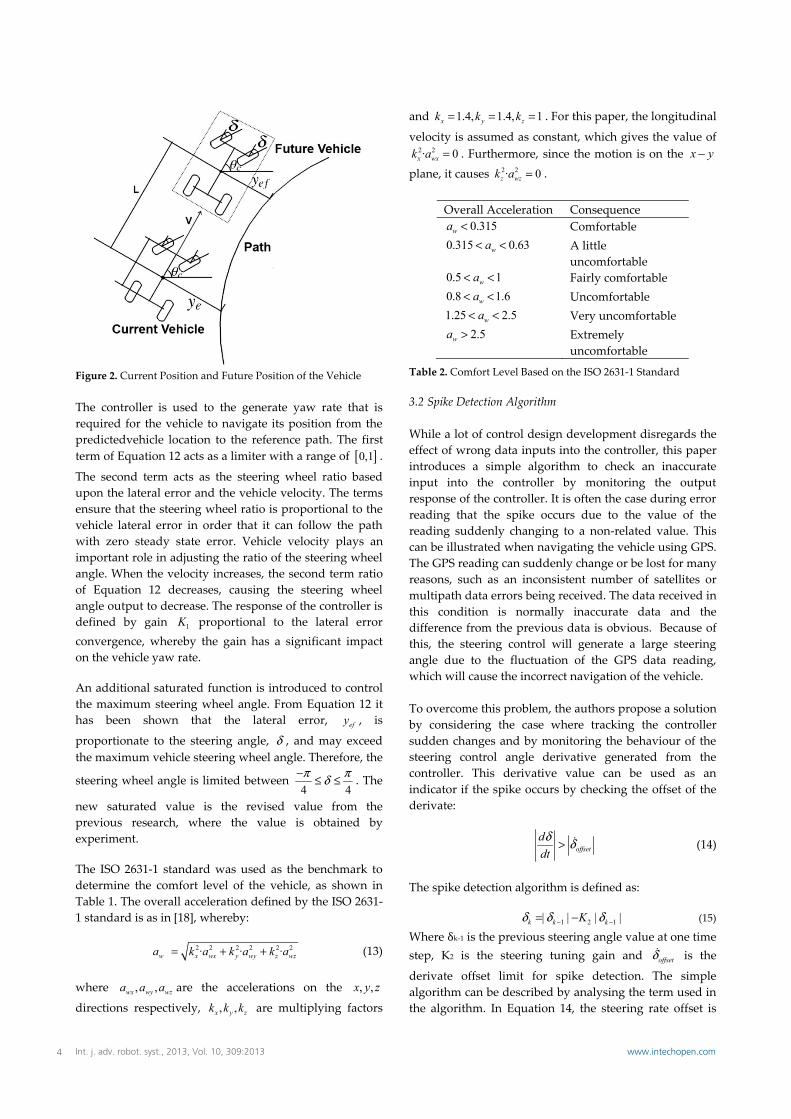
Figure 2. Current Position and Future Position of the Vehicle The controller is used to the generate yaw rate that is required for the vehicle to navigate its position from the predictedvehicle location to the reference path. The first term of Equation 12 acts as a limiter with a range of [ ]0,1 .

The second term acts as the steering wheel ratio based upon the lateral error and the vehicle velocity. The terms ensure that the steering wheel ratio is proportional to the vehicle lateral error in order that it can follow the path with zero steady state error. Vehicle velocity plays an important role in adjusting the ratio of the steering wheel angle. When the velocity increases, the second term ratio of Equation 12 decreases, causing the steering wheel angle output to decrease. The response of the controller is defined by gain 1K proportional to the lateral error convergence, whereby the gain has a significant impact on the vehicle yaw rate. An additional saturated function is introduced to control the maximum steering wheel angle. From Equation 12 it has been shown that the lateral error, efy , is

proportionate to the steering angle, δ , and may exceed the maximum vehicle steering wheel angle. Therefore, the

steering wheel angle is limited between 4 4π πδ− ≤ ≤ . The

new saturated value is the revised value from the previous research, where the value is obtained by experiment. The ISO 2631-1 standard was used as the benchmark to determine the comfort level of the vehicle, as shown in Table 1. The overall acceleration defined by the ISO 2631-1 standard is as in [18], whereby:

2 2 2 2 2 2· · ·w x wx y wy z wza k a k a k a= + + (13)

where , ,wx wy wza a a are the accelerations on the , ,x y z

directions respectively, , ,x y zk k k are multiplying factors

and 1.4, 1.4, 1x y zk k k= = = . For this paper, the longitudinal

velocity is assumed as constant, which gives the value of 2 2· 0x wxk a = . Furthermore, since the motion is on the x y−

plane, it causes 2 2· 0z wzk a = .

Overall Acceleration Consequence 0.315wa < Comfortable

0.315 0.63wa< < A little uncomfortable

0.5 1wa< < Fairly comfortable 0.8 1.6wa< < Uncomfortable 1.25 2.5wa< < Very uncomfortable

2.5wa > Extremely uncomfortable

Table 2. Comfort Level Based on the ISO 2631-1 Standard 3.2 Spike Detection Algorithm While a lot of control design development disregards the effect of wrong data inputs into the controller, this paper introduces a simple algorithm to check an inaccurate input into the controller by monitoring the output response of the controller. It is often the case during error reading that the spike occurs due to the value of the reading suddenly changing to a non-related value. This can be illustrated when navigating the vehicle using GPS. The GPS reading can suddenly change or be lost for many reasons, such as an inconsistent number of satellites or multipath data errors being received. The data received in this condition is normally inaccurate data and the difference from the previous data is obvious. Because of this, the steering control will generate a large steering angle due to the fluctuation of the GPS data reading, which will cause the incorrect navigation of the vehicle. To overcome this problem, the authors propose a solution by considering the case where tracking the controller sudden changes and by monitoring the behaviour of the steering control angle derivative generated from the controller. This derivative value can be used as an indicator if the spike occurs by checking the offset of the derivate:

offsetddt

δδ > (14)

The spike detection algorithm is defined as:

1 2 1| | | |k k kKδ δ δ− −= − (15)

Where δk-1 is the previous steering angle value at one time step, K2 is the steering tuning gain and offsetδ is the

derivate offset limit for spike detection. The simple algorithm can be described by analysing the term used in the algorithm. In Equation 14, the steering rate offset is

4 Int. j. adv. robot. syst., 2013, Vol. 10, 309:2013 www.intechopen.com

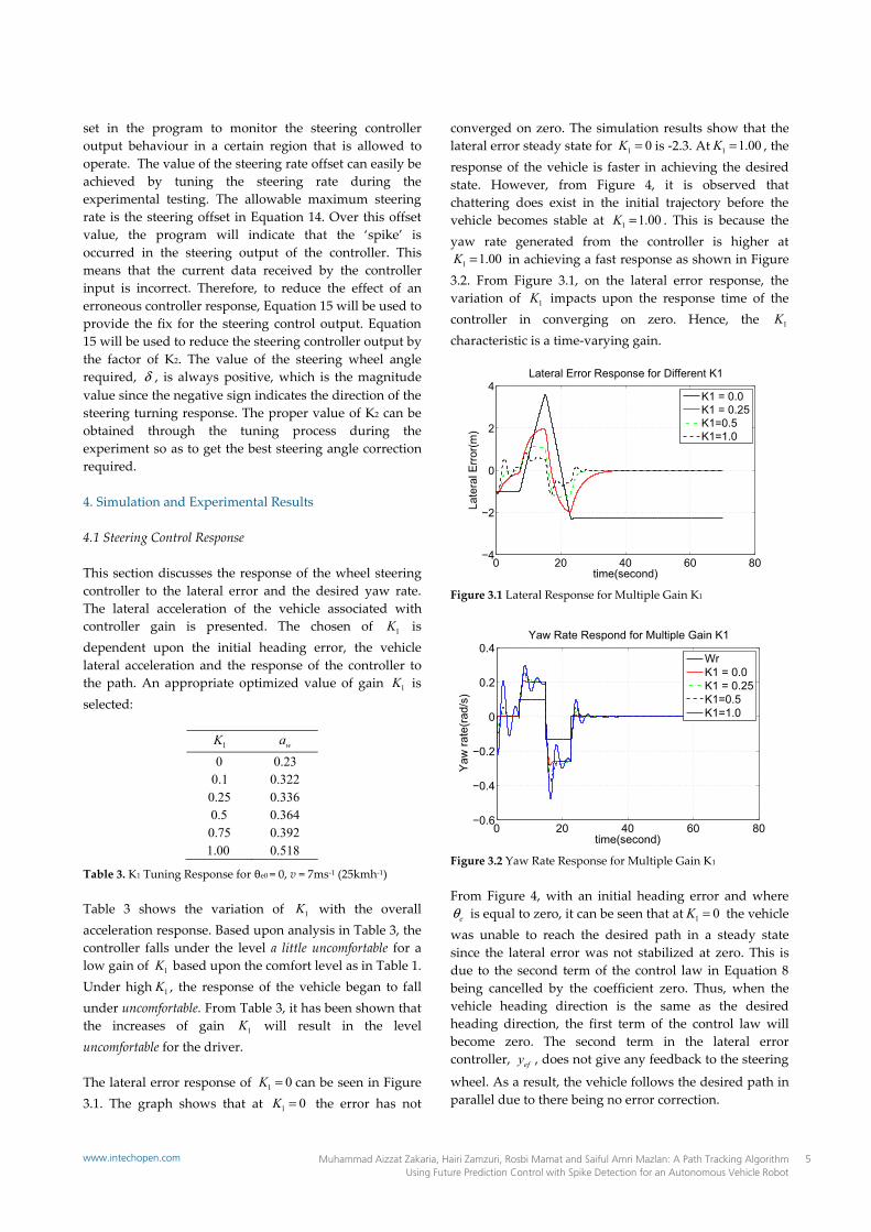
set in the program to monitor the steering controller output behaviour in a certain region that is allowed to operate. The value of the steering rate offset can easily be achieved by tuning the steering rate during the experimental testing. The allowable maximum steering rate is the steering offset in Equation 14. Over this offset value, the program will indicate that the ‘spike’ is occurred in the steering output of the controller. This means that the current data received by the controller input is incorrect. Therefore, to reduce the effect of an erroneous controller response, Equation 15 will be used to provide the fix for the steering control output. Equation 15 will be used to reduce the steering controller output by the factor of K2. The value of the steering wheel angle required, δ , is always positive, which is the magnitude value since the negative sign indicates the direction of the steering turning response. The proper value of K2 can be obtained through the tuning process during the experiment so as to get the best steering angle correction required. 4. Simulation and Experimental Results 4.1 Steering Control Response This section discusses the response of the wheel steering controller to the lateral error and the desired yaw rate. The lateral acceleration of the vehicle associated with controller gain is presented. The chosen of 1K is dependent upon the initial heading error, the vehicle lateral acceleration and the response of the controller to the path. An appropriate optimized value of gain 1K is selected:

1K wa 0 0.23

0.1 0.322 0.25 0.336 0.5 0.364 0.75 0.392 1.00 0.518

Table 3. K1 Tuning Response for θe0 = 0, v = 7ms-1 (25kmh-1) Table 3 shows the variation of 1K with the overall acceleration response. Based upon analysis in Table 3, the controller falls under the level a little uncomfortable for a low gain of 1K based upon the comfort level as in Table 1. Under high 1K , the response of the vehicle began to fall under uncomfortable. From Table 3, it has been shown that the increases of gain 1K will result in the level uncomfortable for the driver. The lateral error response of 1 0K = can be seen in Figure 3.1. The graph shows that at 1 0K = the error has not

converged on zero. The simulation results show that the lateral error steady state for 1 0K = is -2.3. At 1 1.00K = , the response of the vehicle is faster in achieving the desired state. However, from Figure 4, it is observed that chattering does exist in the initial trajectory before the vehicle becomes stable at 1 1.00K = . This is because the yaw rate generated from the controller is higher at

1 1.00K = in achieving a fast response as shown in Figure 3.2. From Figure 3.1, on the lateral error response, the variation of 1K impacts upon the response time of the controller in converging on zero. Hence, the 1K characteristic is a time-varying gain.

Figure 3.1 Lateral Response for Multiple Gain K1

Figure 3.2 Yaw Rate Response for Multiple Gain K1

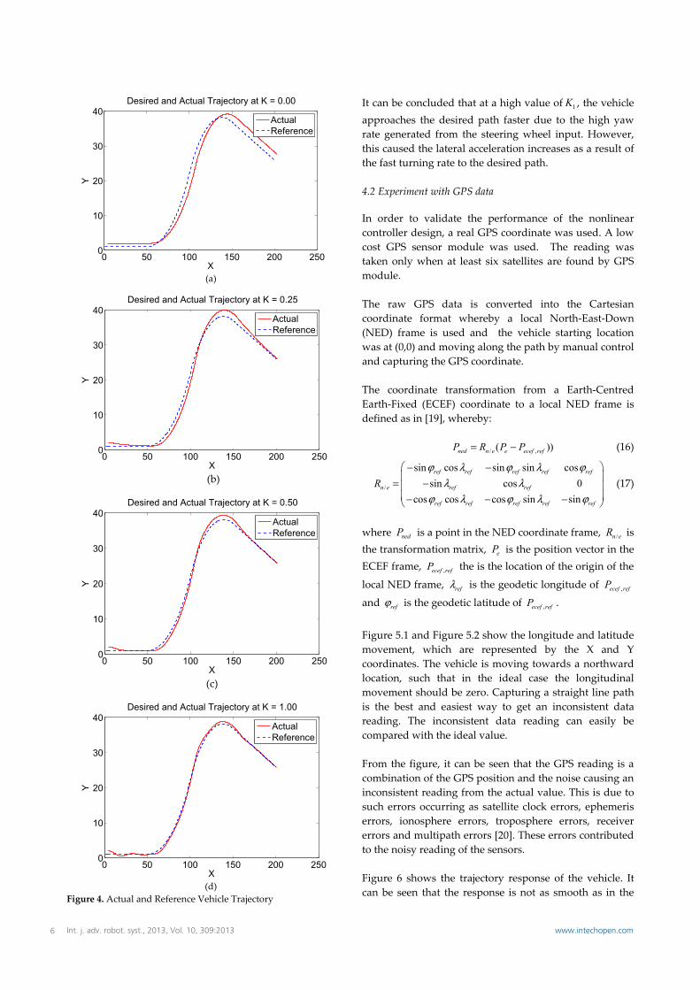
From Figure 4, with an initial heading error and where

eθ is equal to zero, it can be seen that at 1 0K = the vehicle was unable to reach the desired path in a steady state since the lateral error was not stabilized at zero. This is due to the second term of the control law in Equation 8 being cancelled by the coefficient zero. Thus, when the vehicle heading direction is the same as the desired heading direction, the first term of the control law will become zero. The second term in the lateral error controller, efy , does not give any feedback to the steering

wheel. As a result, the vehicle follows the desired path in parallel due to there being no error correction.

5Muhammad Aizzat Zakaria, Hairi Zamzuri, Rosbi Mamat and Saiful Amri Mazlan: A Path Tracking Algorithm Using Future Prediction Control with Spike Detection for an Autonomous Vehicle Robot

www.intechopen.com

(a)

(b)

(c)

(d) Figure 4. Actual and Reference Vehicle Trajectory

It can be concluded that at a high value of 1K , the vehicle approaches the desired path faster due to the high yaw rate generated from the steering wheel input. However, this caused the lateral acceleration increases as a result of the fast turning rate to the desired path. 4.2 Experiment with GPS data In order to validate the performance of the nonlinear controller design, a real GPS coordinate was used. A low cost GPS sensor module was used. The reading was taken only when at least six satellites are found by GPS module. The raw GPS data is converted into the Cartesian coordinate format whereby a local North-East-Down (NED) frame is used and the vehicle starting location was at (0,0) and moving along the path by manual control and capturing the GPS coordinate. The coordinate transformation from a Earth-Centred Earth-Fixed (ECEF) coordinate to a local NED frame is defined as in [19], whereby:

/ ,( ))ned n e e ecef refP R P P= − (16)

/

sin cos sin sin cossin cos 0

cos cos cos sin sin

ref ref ref ref ref

n e ref ref

ref ref ref ref ref

Rϕ λ ϕ λ ϕ

λ λϕ λ ϕ λ ϕ

− − = − − − −

(17)

where nedP is a point in the NED coordinate frame, /n eR is the transformation matrix, eP is the position vector in the ECEF frame, ,ecef refP the is the location of the origin of the

local NED frame, refλ is the geodetic longitude of ,ecef refP

and refϕ is the geodetic latitude of ,ecef refP .

Figure 5.1 and Figure 5.2 show the longitude and latitude movement, which are represented by the X and Y coordinates. The vehicle is moving towards a northward location, such that in the ideal case the longitudinal movement should be zero. Capturing a straight line path is the best and easiest way to get an inconsistent data reading. The inconsistent data reading can easily be compared with the ideal value. From the figure, it can be seen that the GPS reading is a combination of the GPS position and the noise causing an inconsistent reading from the actual value. This is due to such errors occurring as satellite clock errors, ephemeris errors, ionosphere errors, troposphere errors, receiver errors and multipath errors [20]. These errors contributed to the noisy reading of the sensors. Figure 6 shows the trajectory response of the vehicle. It can be seen that the response is not as smooth as in the

6 Int. j. adv. robot. syst., 2013, Vol. 10, 309:2013 www.intechopen.com

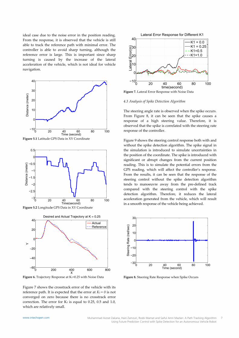
ideal case due to the noise error in the position reading. From the response, it is observed that the vehicle is still able to track the reference path with minimal error. The controller is able to avoid sharp turning, although the reference error is large. This is important since sharp turning is caused by the increase of the lateral acceleration of the vehicle, which is not ideal for vehicle navigation.

Figure 5.1 Latitude GPS Data in XY Coordinate

Figure 5.2 Longitude GPS Data in XY Coordinate

Figure 6. Trajectory Response at K1=0.25 with Noise Data

Figure 7 shows the crosstrack error of the vehicle with its reference path. It is expected that the error at K1 = 0 is not converged on zero because there is no crosstrack error correction. The error for K1 is equal to 0.25, 0.5 and 1.0, which are relatively small.

Figure 7. Lateral Error Response with Noise Data 4.3 Analysis of Spike Detection Algorithm The steering angle rate is observed when the spike occurs. From Figure 8, it can be seen that the spike causes a response of a high steering value. Therefore, it is observed that the spike is correlated with the steering rate response of the controller. Figure 9 shows the steering control response both with and without the spike detection algorithm. The spike signal in the simulation is introduced to simulate uncertainties in the position of the coordinate. The spike is introduced with significant or abrupt changes from the current position reading. This is to simulate the potential errors from the GPS reading, which will affect the controller’s response. From the results, it can be seen that the response of the steering control without the spike detection algorithm tends to manoeuvre away from the pre-defined track compared with the steering control with the spike detection algorithm. Therefore, it reduces the lateral acceleration generated from the vehicle, which will result in a smooth response of the vehicle being achieved.

Figure 8. Steering Rate Response when Spike Occurs

0 200 400 600 800−60

−40

−20

0

20

40

X

Y

Desired and Actual Trajectory at K = 0.25

ActualReference

7Muhammad Aizzat Zakaria, Hairi Zamzuri, Rosbi Mamat and Saiful Amri Mazlan: A Path Tracking Algorithm Using Future Prediction Control with Spike Detection for an Autonomous Vehicle Robot

www.intechopen.com

Figure 9. Vehicle Trajectory Response for Spike Control

5. Conclusion Based upon the simulation carried out, it can be concluded that the proposed nonlinear controller was able to follow the reference path. The vehicle lateral acceleration and path response were observed in order to determine the optimum parameter value of the controller gain. The multiple values of gain are illustrated to present the effect of the gain on the vehicle. The appropriate 1K have been chosen by observing the characteristics of the controller. By selecting a small value of 1K , a slow response of the controller is obtained; however, the small value of the lateral acceleration generated caused the comfort level to increase. If the fast response controller is selected, the comfort level of the vehicle is therefore reduced. Furthermore, the spike detection algorithm is introduced. The simulation results show that the algorithm is able to reduce the unwanted coordinates of the vehicle and achieve a smoother response. The experiment is carried out to monitor the noise characteristics of the GPS sensor. From that, the actual GPS data is fetched to the controller to monitor the controller response if the input data is noisy. The proposed controller is proven to be stable by simulation and experiment from the actual GPS data. However, noisy data will affect the performance of the controller as well. For future research, an Extended Kalman Filter will be investigated in order to estimate the GPS coordinate and reduce the noise in the position reading. 6. Acknowledgments This research is fully supported by the Ministry of Higher Education Malaysia and the Universiti Teknologi Malaysia under ERGS (vote no: 4L033) research grant. The work is also supported by PROTON Holdings Bhd. 7. References [1] Y. Kanayama and Y. Kimura, “A stable tracking

control method for an autonomous mobile robot,” Robotics and Automation, 1990, vol. 1, pp. 384–389, 1990.

[2] R. Fierro and F. L. Lewis, “Control of a Nonholonomic Mobile Robot: Backstepping Kinematics into Dynamics,” vol. 14, no. 3, pp. 149–163, 1997.

[3] S. Lee, “Virtual trajectory in tracking control of mobile robots,” Proceedings 2003 IEEE/ASME International Conference on Advanced Intelligent Mechatronics (AIM 2003), no. Aim, pp. 35–39, 2003.

[4] N. Ouadah, L. Ourak, and F. Boudjema, “Car-like mobile robot oriented positioning by fuzzy controllers,” International Journal of Advanced Robotic Systems, vol. 5, no. 3, pp. 249–256, 2008.

[5] P. Falcone and F. Borrelli, “Predictive active steering control for autonomous vehicle systems,” in IEEE Transactions on Control Systems Technology, Vol. 15, No. 3, May 2007, 2007, vol. 15, no. 3, pp. 566–580.

[6] S. Hima, B. Lusetti, and B. Vanholme, “Trajectory tracking for highly automated passenger vehicles,” in 18th IFAC World Congress, 2011, pp. 12958–12963.

[7] J. Wang, J. Steiber, and B. Surampudi, “Autonomous ground vehicle control system for high-speed and safe operation,” International Journal of Vehicle Autonomous Systems, vol. 7, no. 1, pp. 18–35, 2009.

[8] G. Raffo and G. Gomes, “A predictive controller for autonomous vehicle path tracking,” Intelligent Transportation Systems, IEEE Transactions, vol. 10, no. 1, pp. 92–102, 2009.

[9] V. Subramanian, T. Burks, and W. Dixon, “Sensor fusion using fuzzy logic enhanced kalman filter for autonomous vehicle guidance in citrus groves,” Transactions of the ASAE, vol. 52, no. 5, pp. 1411–1422, 2009.

[10] S. Limsoonthrakul, M. N. Dailey, M. Parnichkunl, C. Science, I. Management, and K. Luang, “Intelligent Vehicle Localization Using GPS, Compass, and Machine Vision,” pp. 3981–3986, 2009.

[11] S. Sukkarieh, E. M. Nebot, and H. F. Durrant-whyte, “A High Integrity IMU/GPS Navigation Loop for Autonomous Land Vehicle Applications,” vol. 15, no. 3, pp. 572–578, 2006.

[12] E. Abbott and D. Powell, “Land-Vehicle Navigation Using GPS,” vol. 87, no. 1, 1999.

[13] V. Milanés, J. E. Naranjo, C. González, J. Alonso, and T. de Pedro, “Autonomous vehicle based in cooperative GPS and inertial systems,” Robotica, vol. 26, no. 05, Mar. 2008.

[14] M. A. Zakaria, H. Zamzuri, S. A. Mazlan, and S. M. H. F. Zainal, “Vehicle Path Tracking Using Future Prediction Steering Control,” Procedia Engineering, vol. 41, pp. 473–479, Jan. 2012.

[15] R. Isermann, “Diagnosis Methods for Electronic Controlled Vehicles,” International Journal of Vehicle Mechanics and Mobility, no. April 2012, pp. 37–41, 2010.

[16] M. Doumiati, O. Sename, L. Dugard, J. Martinez, P. Gaspar, and Z. Szabo, “Integrated vehicle dynamics control via coordination of active front steering and rear braking,” pp. 1–32, 2013.

450 500 550 600 650

−40

−35

−30

−25

−20

−15

−10

−5

0

X

Y

without spike algorithm with spike algorithmreference path

8 Int. j. adv. robot. syst., 2013, Vol. 10, 309:2013 www.intechopen.com

[17] D. Thomas, “Fundamentals of vehicle dynamics,” Society of Automotive Engineering Inc., 1992.

[18] R. Solea and U. Nunes, “Trajectory Planning with Velocity Planner for Fully-Automated Passenger Vehicles,” 2006 IEEE Intelligent Transportation Systems Conference, pp. 474–480, 2006.

[19] G. Cai, B. M. Chen, and T. H. Lee, “Unmanned Rotorcraft Systems,” pp. 23–35, 2011.

[20] E. Nebot and S. Scheding, “Navigation system design,” 2005.

9Muhammad Aizzat Zakaria, Hairi Zamzuri, Rosbi Mamat and Saiful Amri Mazlan: A Path Tracking Algorithm Using Future Prediction Control with Spike Detection for an Autonomous Vehicle Robot

www.intechopen.com