Embed Size (px)
Citation preview

1
A particle confined within a triangular potential well: Airy function, with the use of
Mathematica
Masatsugu Sei Suzuki and Itsuko S. Suzuki
Department of Physics
SUNY at Binghamton
(Date: December 29, 2020)
Julian Seymour Schwinger (February 12, 1918 – July 16, 1994) was a Nobel Prize winning
American theoretical physicist. He is best known for his work on quantum electrodynamics (QED),
in particular for developing a relativistically invariant perturbation theory, and for renormalizing
QED to one loop order. Schwinger was a physics professor at several universities. Schwinger is
recognized as one of the greatest physicists of the twentieth century, responsible for much of
modern quantum field theory, including a variational approach, and the equations of motion for
quantum fields. He developed the first electroweak model, and the first example of confinement
in 1+1 dimensions. He is responsible for the theory of multiple neutrinos, Schwinger terms, and
the theory of the spin-3/2 field.
Photo of Prof. Julian Schwinger.
https://en.wikipedia.org/wiki/Julian_Schwinger
In his book [J. Schwinger, Quantum Mechanics, Symbolism of Atomic Measurements, edited
by B.-G. Englert (Springer, 2001) pages .248-254], the zero and extrema of the Airy function and
the solution of the Schrödinger equation in triangular well potential are extensively discussed,
including numerical calculations of the Airy function. These are very useful to our writing of the

2
present article. As far as we know, in spite of much interest on these topics, we do not find any
article on these topics in standard textbooks of quantum mechanics, except for the Schwinger’s
book and the book of Landau and Lifshitz, partly because of the unique nature of Airy function.
Here, we use the Mathematica Program for the calculations. The use of Mathematica makes it
much easier for us to discuss the prominent nature of Airy function. We note that we first
encountered these topics in the textbook [we used for teaching Phys.421 and Phys.422 (Quantum
Mechanics I and II)]; John S. Townsend, A Modern Quantum Mechanics, second edition
(University Science Books, 2012), Problems 6.9 and 6.10 of page 240;
6.9 Without using exact mathematics - that is, using only arguments of curvature, symmetry, and
semiquantitative estimates of wavelength – sketch the energy eigenfunctions for the ground state,
first excited state, and second excited state of a particle in the potential energy well ( )V z a z .
This potential energy has been suggested as arising from the force exerted by one quark on another
quark.
In the physical sciences, the Airy function (or Airy function of the first kind) Ai(x) is a special
function named after the British astronomer George Biddell Airy (1801–1892). The function Ai(x)
and the related function Bi(x), are linearly independent solutions to the differential equation
2
2
( )( ) 0
d y xxy x
dx , (1)
known as the Airy equation or the Stokes equation. This is the simplest second-order linear
differential equation with a turning point (a point where the character of the solutions changes
from oscillatory to exponential). The Airy function is the solution to the time-independent
Schrödinger equation for a particle confined within a triangular potential well.
1. Schrödinger equation with a triangular potential well
We consider the Hamiltonian H of a particle confined within inside a triangular potential well,
which is given by
21ˆ ˆ ˆ( )2
zH p V zm
, (2)
with the triangular well potential
ˆ ˆ( )V z a z , (3)
where m is the mass of particle, and ˆzp is the linear momentum along the z axis.
3
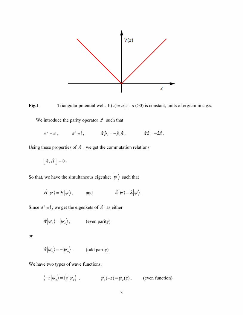
Fig.1 Triangular potential well. ( )V z a z . a (>0) is constant, units of erg/cm in c.g.s.
We introduce the parity operator such that
ˆ ˆ , 2 ˆˆ 1 , ˆ ˆ ˆ ˆz zp p , ˆ ˆˆ ˆz z .
Using these properties of , we get the commutation relations
ˆˆ , 0H .
So that, we have the simultaneous eigenket such that
H E , and .
Since 2 ˆˆ 1 , we get the eigenkets of as either
ˆe e , (even parity)
or
ˆo o . (odd parity)
We have two types of wave functions,
e ez z , ( ) ( )e ez z , (even function)

4
and
O oz z , ( ) ( )o oz z , (odd function)
In general, the continuity of ( )z and ( )d z
dz
at z= 0 can be obtained as,
(0) 0e
d
dz , (0) 0o .
for the even function and the odd function, respectively.
Based on these, here we discuss the one-dimensional time-independent Schrödinger equation
with the triangular well; ˆ ˆ( )V z a z ,
2
2 2
( ) 2( ) ( ) 0
d z mE a z z
dz
ℏ. (4)
where ℏ is a Planck constant, E is the energy eigenvalue, a (>0) is constant, units of [erg/cm] in
c.g.s. For simplicity, we define the dimensionless parameters and x, where
21/3
2( )2
aE
m
ℏ, and
21/3( )
2z x
ma
ℏ. (5)
Then, the Schrödinger equation can be rewritten as
2
2
( )( ) ( ) 0
d xx x
dx
. (6)
Note that the classical turning point is defined by
clx ,
where is the normalized energy eigenvalue.
2. Energy eigenvalue for wave function with even parity
The wave function should be either an even function (even parity) or an odd function (odd
parity) with respect to x = 0. Note that the classical limit is clx x . In other words, in classically

5
the wave function should be zero for clx x . However, in quantum mechanics, as will be shown
later, the wave function is not zero above the classical limit because of the quantum tunneling
effect. For simplicity, for 0x , we use
y x , ( y )
2
2( ) ( ) 0
dy y y
dy . (7)
The solution of the differential equation is obtained as
( )y Ai(y) or Bi(y)
Note that conventionally, we use
Ai(y)=AirAi[y],
Bi(y)=AirBi[y],
Ai’(y)= AirAiPrime[y],
in Mathematica. The function Bi(y) diverges in the large limit of y . So that, we do not adopt
this function as our solution. Note that we have a new function Ai( ) Ai( )y y x , where
'( ) Ai( ) [ AirAiPrime( )]d
Ai y y ydy
Since the potential ( )V z a z is symmetric with respect to z = 0, the wave function is either
symmetric (even parity) or antisymmetric (odd parity) with respect to y=0 (or x = 0).
For the odd parity,
Ai( ) 0y , at ( )y o p , (p =1, 2, 3, …)
with the energy eigenvalue ( )o p ( 0 ). Note that ( ) 0o p .
TABLE 1: The odd parity: ( )o p vs p (p=1, 2, 3,….). 2 1n p .
p n o(p)

6
__________________________
1 1 -2.33811
2 3 -4.08795
3 5 -5.52056
4 7 -6.78671
5 9 -7.94413
6 11 -9.02265
7 13 -10.0402
8 15 -11.0085
9 17 -11.936
10 19 -12.8288
11 21 -13.6915
12 23 -14.5278
13 25 -15.3408
14 27 -16.1327
15 29 -16.9056
Fig.2 Airy function Ai(y) as a function of y. Ai(y) takes zero at ( )y o p with p = 1, 2, 3,.... .
Note that ( ) 0.o p The quantum number n (defined later) is related to p as 2 1n p .
3 Energy eigenvalue for the wave function with even parity
For the even parity, we have
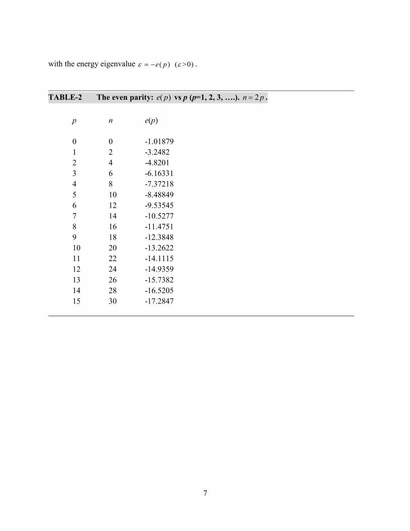
Ai'( ) 0y , at ( )y e p , (p =0,1, 2, 3, …))
7
with the energy eigenvalue ( ) ( >0)e p .
____________________________________________________________________________
TABLE-2 The even parity: ( )e p vs p (p=1, 2, 3, ….). 2n p .
p n e(p)
0 0 -1.01879
1 2 -3.2482
2 4 -4.8201
3 6 -6.16331
4 8 -7.37218
5 10 -8.48849
6 12 -9.53545
7 14 -10.5277
8 16 -11.4751
9 18 -12.3848
10 20 -13.2622
11 22 -14.1115
12 24 -14.9359
13 26 -15.7382
14 28 -16.5205
15 30 -17.2847
____________________________________________________________________________
8
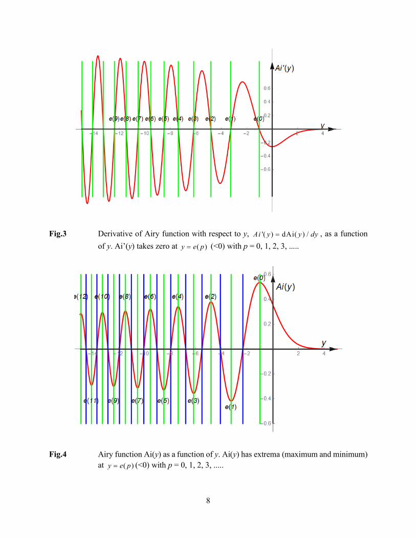
Fig.3 Derivative of Airy function with respect to y, '( ) dAi( ) /Ai y y dy , as a function
of y. Ai’(y) takes zero at ( )y e p (<0) with p = 0, 1, 2, 3, .....
Fig.4 Airy function Ai(y) as a function of y. Ai(y) has extrema (maximum and minimum)
at ( )y e p (<0) with p = 0, 1, 2, 3, .....

9
4. Construction of wave function (I)
4.1 Wave function with even parity
The Airy function Ai(x) takes a maximum at ( ) (<0)x e p . The new wave function with even
parity can be constructed from the shift the graph of Ai(x) for ( )x e p (denoted by blue line) to
the right by ( )e p . It is not allowed to use the Airy function for ( )x e p (denoted by the blue
line). The value of ( )e p is called the classical limit (classical turning point). The wave function
is an even function of x with respect x = 0. So that, the wave function for x<0 is newly obtained
graph from that for x>0 reflected about the y-axis (at x = 0). The resulting wave function should
be normalized as
1( , ) [ ( )]
2 Ce( )e
x p Ai x e pp
, (8)
with
2
( )
( ) [ ( )]e p
Ce p Ai x dx
. (9)
The resulting function is symmetric with respect to x = 0.
4.2 Wave function with odd parity
The Airy function becomes zero at ( ) ( 0)x o p . The new wave function with odd parity can
be constructed from the shift the graph of Ai(x) for ( )x o p (denoted by blue line) to the right by
( )o p . We do not use the Airy function for ( )x o p (denoted by the blue line). The value of ( )o p
is called the classical limit. The wave function is an odd function of x with respect x = 0. So that,
the wave function for x<0 is newly obtained from the rotation of this graph for x>0 through 180°
about the origin. The resulting wave function should be normalized as
1( , ) sgn( )Ai[ ( )]
2 Co( )o
x p x x o pp
, (p=0, 1, 2, …) (10)
with
2
( )
( ) [ ( )]o p
Co p Ai x dx
. (11)
4.3 Quantum number n

10
We introduce the quantum number n as follows.
TABLE 3: Quantum number n
The energy eigenvalue, quantum number n 1
2 ( )eC p
( 0) ( 0) 1.01879n e p n = 0 (even), 1.30784
(1) ( 1) 2.33811o p , 1n (odd) 1.00841
(2) (1) 3.2482e , 2n (even) 0.93634
(3) (2) 4.08795o , 3n (odd) 0.880459
(4) (2) 4.8201e 4n (even) 0.84666
(5) (3) 5.52056o , 5n (odd) 0.817272
(6) (3) 6.16331e , 6n (even) 0.795805
(7) (4) 6.78671o , 7n (odd) 0.776315
(8) (4) 7.37218e , 8n (even) 0.760814
(9) (5) 7.94413o , 9n (odd) 0.746416
(10) (5) 8.48849e , 10n (even) 0.734395
(11) (6) 9.02265o , 11n (odd) 0.72307
(12) (6) 9.53545e , 12n (even) 0.713312
(13) (7) 10.0402o , 13n (odd) 0.70403
(14) (7) 10.5277e , 14n (even) 0.695853
(15) (8) 11.0085o , 15n (odd) 0.688022
(16) (8) 11.4751e , 16n (even) 0.681009
(17) (9) 11.936o , 18n (odd) 0.674257
(18) (9) 12.3848e , 19n (even) 0.668133
(19) (10) 12.8288o , 20n (even) 0.662213
(20) (10) 13.2622e , 21n (even) 0.65679
5. Construction of wave function II: examples
5.1 Wave function with n = 0 (even parity)
In order to construct the wave function with n = 0, first the part of ( )Ai y denoted by the red
line ( (0)y e ) is shifted to the positive y direction so that the green line moves to the 0y .
1
2 ( )oC p

11
Fig.5(a) Airy function Ai(y) as a function of y. The red line for (0)y e contributes to the
wave function at n = 0 (even parity). (0)y e is denoted by the green line. The
Airy function Ai(y) for (0)y e is shifted such that the green line reaches the origin
(y = 0).
Fig.5(b) Construction of wave function for 0x from the folding of the wave function for
0x along the vertical axis at x = 0. So that, the resulting wave function (n = 0,
the even function) is symmetric with respect to x = 0.
y
Ai y
e 0
Shift
15 14 13 12 11 10 9 8 7 6 5 4 3 2 1 1 2 3 4 5
0.5
0.4
0.3
0.2
0.1
0.1
0.2
0.3
0.4
0.5
x
n 0,x
Folding
10 9 8 7 6 5 4 3 2 1 1 2 3 4 5 6 7 8 9 10
0.1
0.1
0.2
0.3
0.4
0.5
12
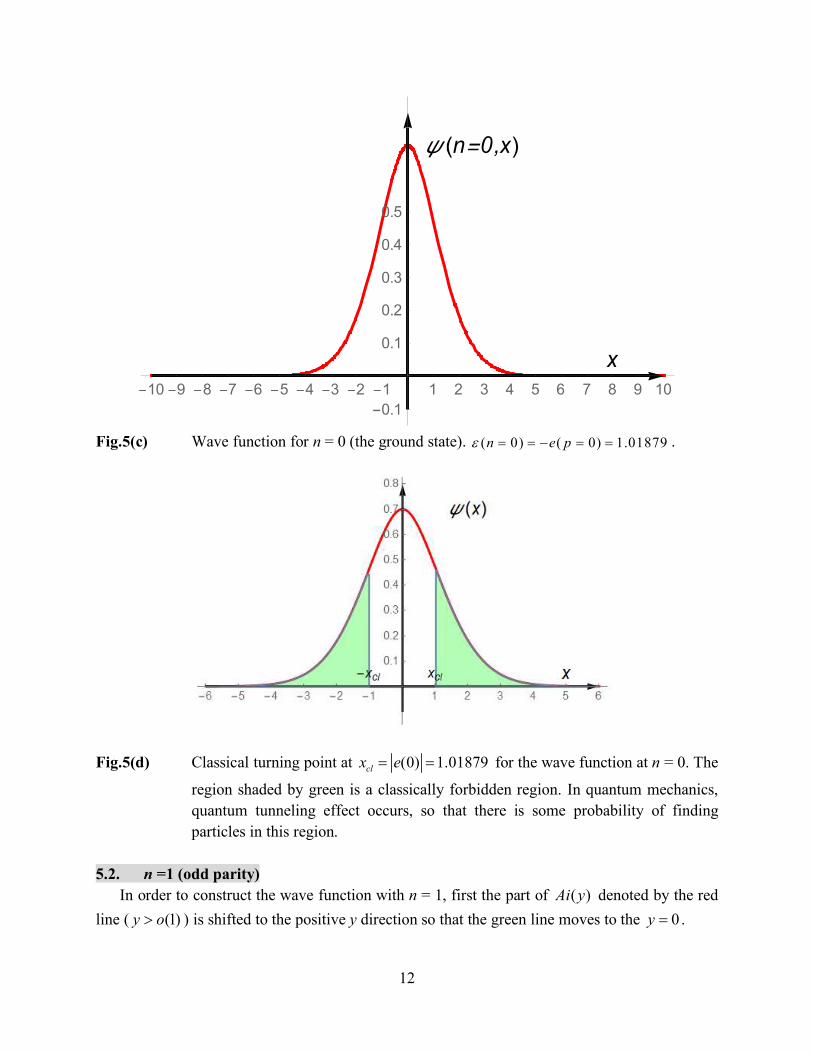
Fig.5(c) Wave function for n = 0 (the ground state). ( 0) ( 0) 1.01879n e p .
Fig.5(d) Classical turning point at (0) 1.01879clx e for the wave function at n = 0. The
region shaded by green is a classically forbidden region. In quantum mechanics,
quantum tunneling effect occurs, so that there is some probability of finding
particles in this region.
5.2. n =1 (odd parity)
In order to construct the wave function with n = 1, first the part of ( )Ai y denoted by the red
line ( (1)y o ) is shifted to the positive y direction so that the green line moves to the 0y .
x
n 0,x
10 9 8 7 6 5 4 3 2 1 1 2 3 4 5 6 7 8 9 10
0.1
0.1
0.2
0.3
0.4
0.5
13
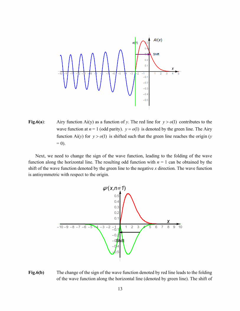
Fig.6(a): Airy function Ai(y) as a function of y. The red line for (1)y o contributes to the
wave function at n = 1 (odd parity). (1)y o is denoted by the green line. The Airy
function Ai(y) for (1)y o is shifted such that the green line reaches the origin (y
= 0).
Next, we need to change the sign of the wave function, leading to the folding of the wave
function along the horizontal line. The resulting odd function with n = 1 can be obtained by the
shift of the wave function denoted by the green line to the negative x direction. The wave function
is antisymmetric with respect to the origin.
Fig.6(b) The change of the sign of the wave function denoted by red line leads to the folding
of the wave function along the horizontal line (denoted by green line). The shift of
x
x,n 1
Shift
10 9 8 7 6 5 4 3 2 1 1 2 3 4 5 6 7 8 9 10
0.5
0.4
0.3
0.2
0.1
0.1
0.2
0.3
0.4
0.5
14
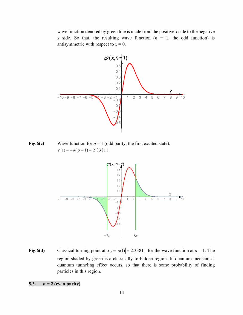
wave function denoted by green line is made from the positive x side to the negative
x side. So that, the resulting wave function (n = 1, the odd function) is
antisymmetric with respect to x = 0.
Fig.6(c) Wave function for n = 1 (odd parity, the first excited state).
(1) ( 1) 2.33811o p .
Fig.6(d) Classical turning point at (1) 2.33811clx o for the wave function at n = 1. The
region shaded by green is a classically forbidden region. In quantum mechanics,
quantum tunneling effect occurs, so that there is some probability of finding
particles in this region.
5.3. n = 2 (even parity)
x
x,n 1
10 9 8 7 6 5 4 3 2 1 1 2 3 4 5 6 7 8 9 10
0.5
0.4
0.3
0.2
0.1
0.1
0.2
0.3
0.4
0.5
15
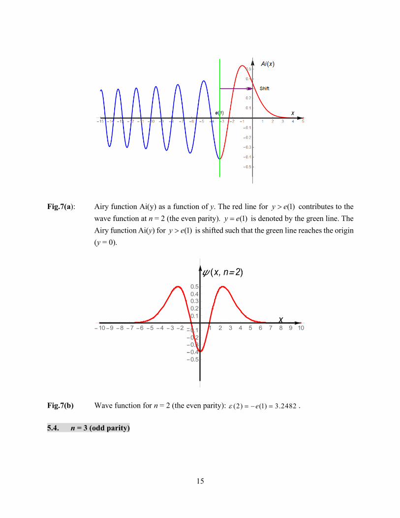
Fig.7(a): Airy function Ai(y) as a function of y. The red line for (1)y e contributes to the
wave function at n = 2 (the even parity). (1)y e is denoted by the green line. The
Airy function Ai(y) for (1)y e is shifted such that the green line reaches the origin
(y = 0).
Fig.7(b) Wave function for n = 2 (the even parity): (2) (1) 3.2482e .
5.4. n = 3 (odd parity)
x
x, n 2
10 9 8 7 6 5 4 3 2 1 1 2 3 4 5 6 7 8 9 10
0.5
0.4
0.3
0.2
0.1
0.1
0.2
0.30.4
0.5

16
Fig.8(a): Airy function Ai(y) as a function of y. The red line for (2)y o contributes to the
wave function at n = 3 (the odd parity). (2)y o is denoted by the green line. The
Airy function Ai(y) for (2)y o is shifted such that the green line reaches the origin
(y = 0).
Fig.8(b) Wave function for n = 3 (odd parity), which is asymmetric with respect to the origin.
(3) (2) 4.08795o . (2) 4.08795clx o .
5.5. n =4 (even parity)
x
x, n 3
10 9 8 7 6 5 4 3 2 1 1 2 3 4 5 6 7 8 9 10
0.5
0.4
0.3
0.2
0.1
0.1
0.2
0.3
0.4
0.5

17
Fig.9(a): Airy function Ai(y) as a function of y. The red line for (2)y e contributes to the
wave function at n = 4 (the even parity). (2)y e is denoted by the green line. The
Airy function Ai(y) for (2)y e is shifted such that the green line reaches the origin
(y = 0).
Fig.9(b) Wave function for n = 4 (even parity). (4) (2) 4.8201e .
(2) 4.8201clx e .
5.6. n =5 (odd parity)
x
x, n 4
10 9 8 7 6 5 4 3 2 1 1 2 3 4 5 6 7 8 9 10
0.5
0.4
0.3
0.2
0.1
0.1
0.2
0.3
0.4
0.5
18
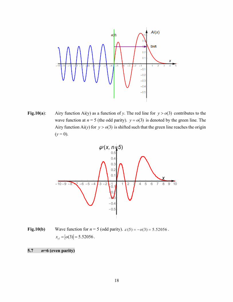
Fig.10(a): Airy function Ai(y) as a function of y. The red line for (3)y o contributes to the
wave function at n = 5 (the odd parity). (3)y o is denoted by the green line. The
Airy function Ai(y) for (3)y o is shifted such that the green line reaches the origin
(y = 0).
Fig.10(b) Wave function for n = 5 (odd parity). (5) (3) 5.52056o .
(3) 5.52056clx o .
5.7 n=6 (even parity)
x
x, n 5
10 9 8 7 6 5 4 3 2 1 1 2 3 4 5 6 7 8 9 10
0.5
0.4
0.3
0.2
0.1
0.1
0.2
0.3
0.4
0.5
19
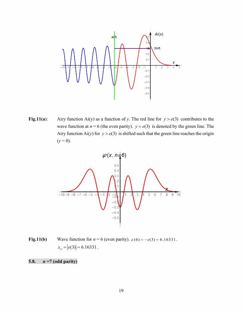
Fig.11(a): Airy function Ai(y) as a function of y. The red line for (3)y e contributes to the
wave function at n = 6 (the even parity). (3)y e is denoted by the green line. The
Airy function Ai(y) for (3)y e is shifted such that the green line reaches the origin
(y = 0).
Fig.11(b) Wave function for n = 6 (even parity). (6) (3) 6.16331e .
(3) 6.16331clx e .
5.8. n =7 (odd parity)
20
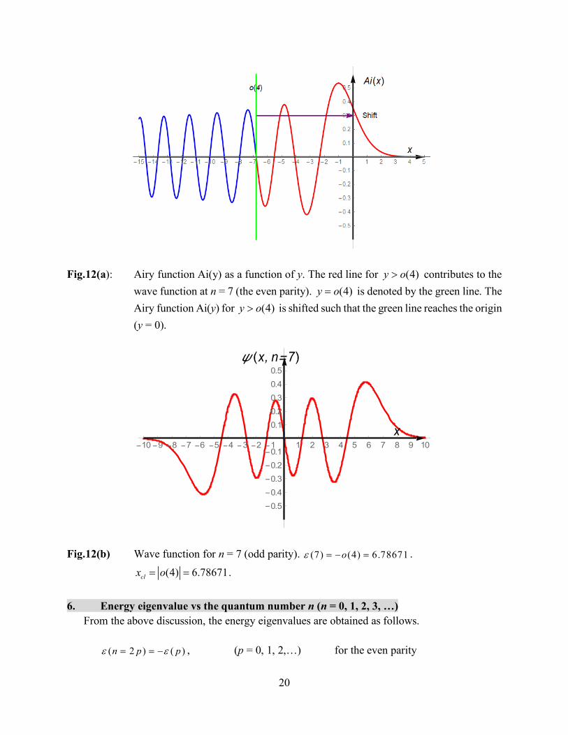
Fig.12(a): Airy function Ai(y) as a function of y. The red line for (4)y o contributes to the
wave function at n = 7 (the even parity). (4)y o is denoted by the green line. The
Airy function Ai(y) for (4)y o is shifted such that the green line reaches the origin
(y = 0).
Fig.12(b) Wave function for n = 7 (odd parity). (7) (4) 6.78671o .
(4) 6.78671clx o .
6. Energy eigenvalue vs the quantum number n (n = 0, 1, 2, 3, …)
From the above discussion, the energy eigenvalues are obtained as follows.
( 2 ) ( )n p p , (p = 0, 1, 2,…) for the even parity
x
x, n 7
10 9 8 7 6 5 4 3 2 1 1 2 3 4 5 6 7 8 9 10
0.5
0.4
0.3
0.2
0.1
0.1
0.2
0.3
0.4
0.5

21
( 2 1) ( )n p o p (p = 1, 2, 3,…) for the odd parity.
According to Schwinger, the energy eigen value is expressed by
2/3 4/33 1 1 1 3 1( ) [ ( )] [ ( 1) ][ ( )]
4 2 48 8 4 2
nn n n
, (Schwinger).
or
2/3
3 1( ) ( )
4 2n n
≃ . (approximation) (12)
Here we make a plot of the energy eigenvalue vs the quantum number n (n = 0, 1, 2, 3, …). For
comparison, we also make a plot of the prediction by Schwinger. It is found that these are in
excellent agreement with each other.
Fig.13 Energy eigenvalue ( )n vs n. Even parity (denoted by red dots). Odd parity
(denoted by blue dots). The solid line is described by the equation derived by
Schwinger [Eq.(12)].
7. Probability vs the quantum number
7.1 Probability vs x for n = 0 (even parity); ground state
22
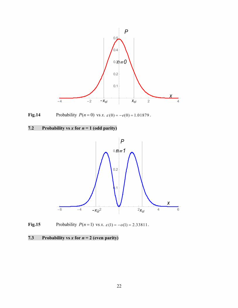
Fig.14 Probability ( 0)P n vs x. (0) (0) 1.01879e .
7.2 Probability vs x for n = 1 (odd parity)
Fig.15 Probability ( 1)P n vs x. (1) (1) 2.33811o .
7.3 Probability vs x for n = 2 (even parity)
n 0
x
P
xclxcl4 2 2 4
0.1
0.2
0.3
0.4
0.5
n 1
x
P
xclxcl6 4 2 2 4 6
0.1
0.2
0.3
23
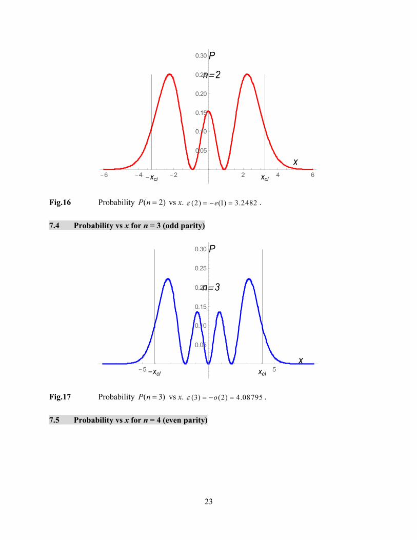
Fig.16 Probability ( 2)P n vs x. (2) (1) 3.2482e .
7.4 Probability vs x for n = 3 (odd parity)
Fig.17 Probability ( 3)P n vs x. (3) (2) 4.08795o .
7.5 Probability vs x for n = 4 (even parity)
n 2
x
P
xclxcl6 4 2 2 4 6
0.05
0.10
0.15
0.20
0.25
0.30
n 3
x
P
xclxcl5 5
0.05
0.10
0.15
0.20
0.25
0.30

24
Fig.18 Probability ( 4)P n vs x. (4) (2) 4.8201e .
7.6 Probability vs x for n = 5 (odd parity)
Fig.19 Probability ( 5)P n vs x. (5) (3) 5.52056o .
7.7 Probability vs x for n = 6 (even parity)
n 4
x
P
xclxcl5 5
0.05
0.10
0.15
0.20
0.25
n 5
x
P
xclxcl5 5
0.05
0.10
0.15
0.20
0.25
25
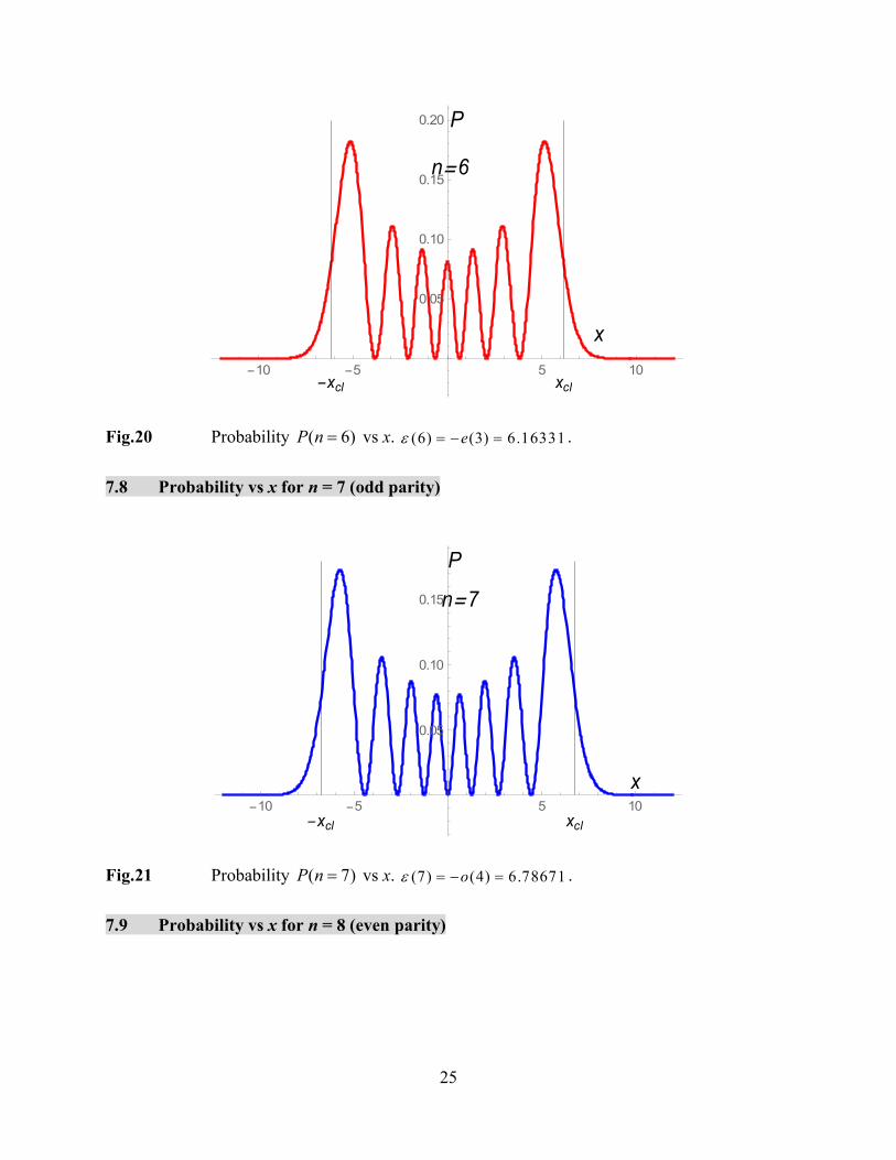
Fig.20 Probability ( 6)P n vs x. (6) (3) 6.16331e .
7.8 Probability vs x for n = 7 (odd parity)
Fig.21 Probability ( 7)P n vs x. (7) (4) 6.78671o .
7.9 Probability vs x for n = 8 (even parity)
n 6
x
P
xclxcl10 5 5 10
0.05
0.10
0.15
0.20
n 7
x
P
xclxcl10 5 5 10
0.05
0.10
0.15
26
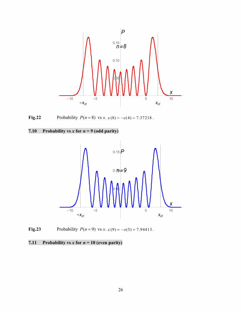
Fig.22 Probability ( 8)P n vs x. (8) (4) 7.37218e .
7.10 Probability vs x for n = 9 (odd parity)
Fig.23 Probability ( 9)P n vs x. (9) (5) 7.94413o .
7.11 Probability vs x for n = 10 (even parity)
n 8
x
P
xclxcl10 5 5 10
0.05
0.10
0.15
n 9
x
P
xclxcl
10 5 5 10
0.05
0.10
0.15

27
Fig.23 Probability ( 10)P n vs x. (10) (5) 8.48849e .
8. Classical turning point and the escape probability
clx is the classical turning point. The wave function does not vanish beyond the classical
turning point, but it dies out exponentially as x . Notice, however, that when n is large, the
excursions outside the turning points are small compared to the classical amplitude.
Here we discuss the escape probability for finding particle beyond the classical turning limit
2
0
[ ( )] 0.0669875LC Ai x dx
, (13)
2
0
2
( )
[ ( )]
( 2 1)( )
[ ( )]
Lescape
e
e p
Ai x dxC
P n pC p
Ai x dx
, for the even parity (14)
and
2
0
2
( )
[ ( )]
( 2 )( )
[ ( )]
Lescape
o
o p
Ai x dxC
P n pC p
Ai x dx
, for the odd parity (15)
n 10
x
P
xclxcl
10 5 5 10
0.05
0.10
0.15
28
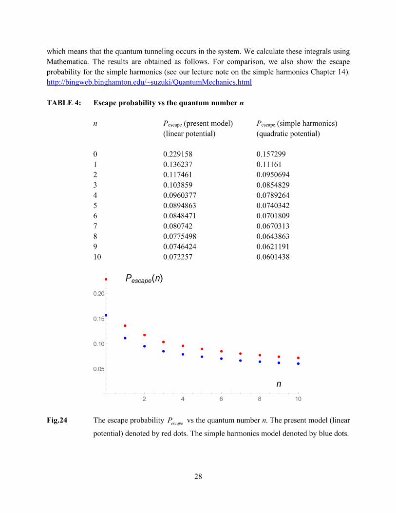
which means that the quantum tunneling occurs in the system. We calculate these integrals using
Mathematica. The results are obtained as follows. For comparison, we also show the escape
probability for the simple harmonics (see our lecture note on the simple harmonics Chapter 14).
http://bingweb.binghamton.edu/~suzuki/QuantumMechanics.html
TABLE 4: Escape probability vs the quantum number n
n Pescape (present model) Pescape (simple harmonics)
(linear potential) (quadratic potential)
0 0.229158 0.157299
1 0.136237 0.11161
2 0.117461 0.0950694
3 0.103859 0.0854829
4 0.0960377 0.0789264
5 0.0894863 0.0740342
6 0.0848471 0.0701809
7 0.080742 0.0670313
8 0.0775498 0.0643863
9 0.0746424 0.0621191
10 0.072257 0.0601438
Fig.24 The escape probability escapeP vs the quantum number n. The present model (linear
potential) denoted by red dots. The simple harmonics model denoted by blue dots.
n
Pescape n
2 4 6 8 10
0.05
0.10
0.15
0.20
29
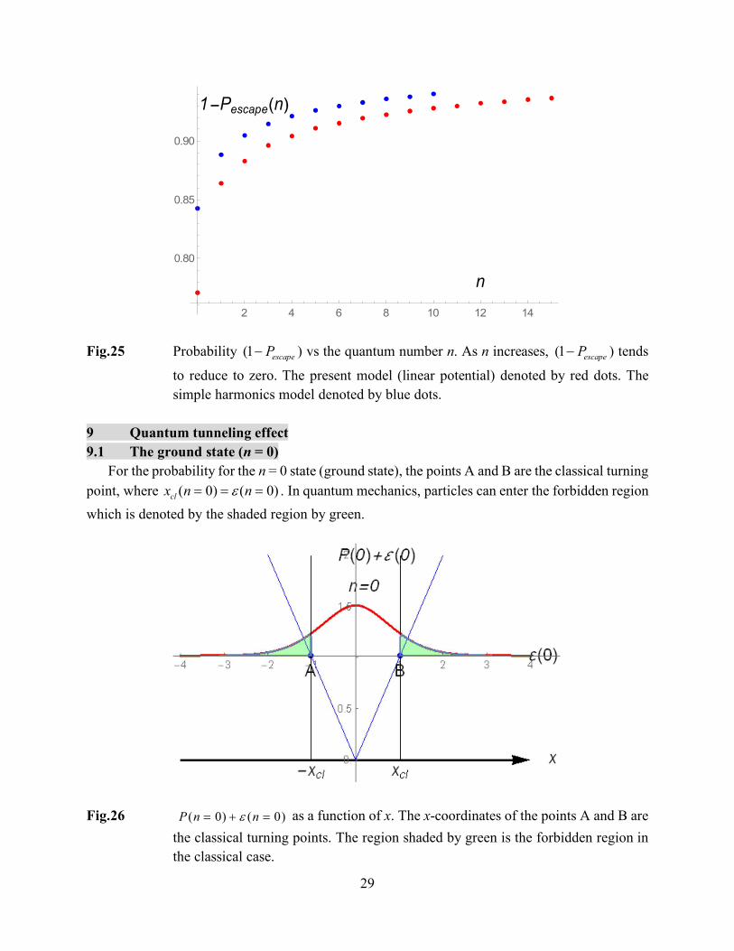
Fig.25 Probability (1 escapeP ) vs the quantum number n. As n increases, (1 escapeP ) tends
to reduce to zero. The present model (linear potential) denoted by red dots. The
simple harmonics model denoted by blue dots.
9 Quantum tunneling effect
9.1 The ground state (n = 0)
For the probability for the n = 0 state (ground state), the points A and B are the classical turning
point, where ( 0) ( 0)clx n n . In quantum mechanics, particles can enter the forbidden region
which is denoted by the shaded region by green.
Fig.26 ( 0) ( 0)P n n as a function of x. The x-coordinates of the points A and B are
the classical turning points. The region shaded by green is the forbidden region in
the classical case.
n
1 Pescape n
2 4 6 8 10 12 14
0.80
0.85
0.90
30
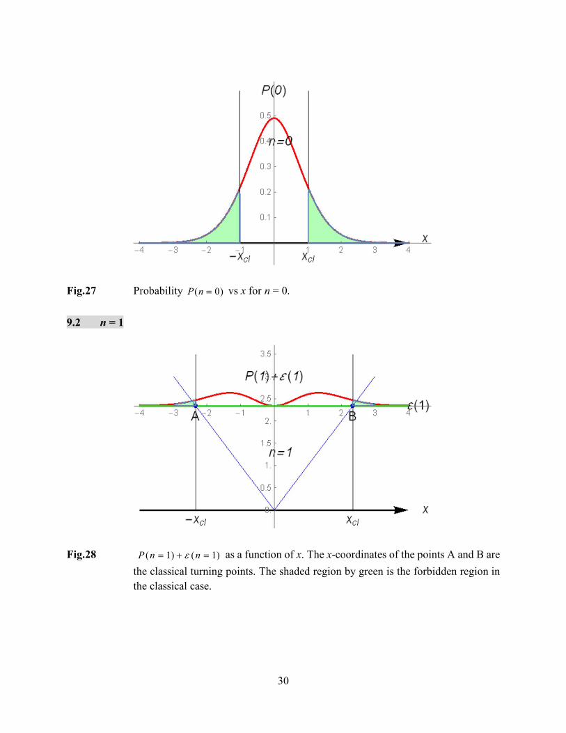
Fig.27 Probability ( 0)P n vs x for n = 0.
9.2 n = 1
Fig.28 ( 1) ( 1)P n n as a function of x. The x-coordinates of the points A and B are
the classical turning points. The shaded region by green is the forbidden region in
the classical case.
31
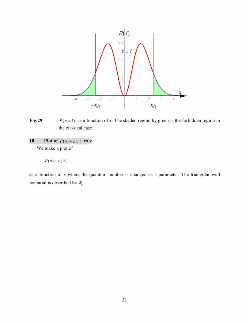
Fig.29 ( 1)P n as a function of x. The shaded region by green is the forbidden region in
the classical case.
10. Plot of ( ) ( )P n n vs x
We make a plot of
( ) ( )P n n
as a function of x where the quantum number is changed as a parameter. The triangular well
potential is described by clx
32
(a)
(b)
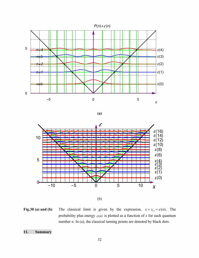
Fig.30 (a) and (b) The classical limit is given by the expression, ( )clx x n . The
probability plus energy ( )n is plotted as a function of x for each quantum
number n. In (a), the classical turning points are denoted by black dots.
11. Summary
x
P n n
0 55
0
5
0
2
4
1
3
n 0
n 2
n 4
n 1
n 3
x0 5 105100
5
10
0
2
4
6
810121416
1
3

33
Using the properties of the Airy function, the Schrödinger equation of a particle in the presence
of a linear triangular well can be solved exactly. It is surprising for us that a part of the Airy
function is a solution of the Schrödinger equation. The even parity and the odd parity of the wave
function is related to the symmetry of the linear triangular well potential with respect to the origin.
We also realize the similarity between the present model and the simple harmonics. The escape
probability vs the quantum number is essentially similar between these two models.
__________________________________________________________________________
REFERENCES
L.D. Landau and E.M. Lifshitz, Quantum Mechanics (Non-relativistic Theory), 3rd edition
(Pergamon, 1977).
J. Schwinger, Quantum Mechanics, Symbolism of Atomic Measurements, edited by B.-G. Englert
(Springer, 2001).
J.J. Sakurai and J. Napolitano, Modern Quantum Mechanics (Pearson, 2011).
J.S. Townsend, A Modern Approach to Quantum Mechanics, Second edition (University Science
Book, 2012).
A. Goswami, Quantum Mechanics, second edition (WCB, 2003).
R. Shankar, Principles of Quantum Mechanics, second edition (Kluwer Academics/Plenum, 1994).
Y. Peleg, R. Pnini, and E. Zaarur, Schaum’s outline of Theory and Problems of Quantum
Mechanics, second edition (Pearson, 2011).
O. Vallée and M. Soares, Airy Functions and Application, Imperial College (World Scientific,
2004).
______________________________________________________________________________
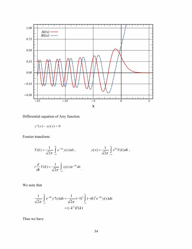
APPENDIX-I Property of Airy function
The Airy function Ai(x) is a special function named after British astronomer George Biddell
Airy. The function Ai(x) and the related function Bi(x), which is also called the Airy function.
34
Differential equation of Airy function
"( ) ( ) 0y x xy x
Fourier transform:
1( ) ( )
2
ikxY k e y x dx
, 1
( ) ( )2
ikxy x e Y k dk
,
1( ) ( )
2
ikxdi Y k xy x e dx
dk
.
We note that
2 2
2
1 1''( ) ( 1) ( ) ( )
2 2
( ) ( )
ikx ikxe y x dx ik e y x dx
k Y k
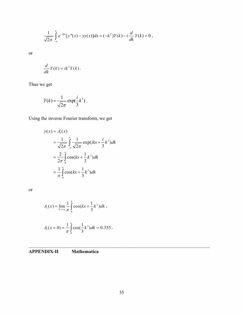
Thus we have
35
21[ ''( ) ( )] ( ) ( ) ( ) 0
2
ikx de y x xy x dx k Y k i Y k
dk
,
or
2( ) ( )d
Y k ik Y kdk
.
Thus we get
31( ) exp( )
32
iY k k
.
Using the inverse Fourier transform, we get
3
3
0
3
0
( ) ( )
1 1exp( )
32 2
2 1cos( )
2 3
1 1cos( )
3
iy x A x
iikx k dk
kx k dk
kx k dk
or
3
0
1 1( ) lim cos( )
3
b
ib
A x kx k dk
,
3
0
1 1( 0) cos( ) 0.355
3iA x k dk
.
____________________________________________________________________________
APPENDIX-II Mathematica

36