A numerical approach to a multi-objective optimal ... · In the case of multi-item inventory models, it is possible to study each item separately as long as there is no interactions

Computers and Mathematics with Applications 55 (2008) 1794–1807www.elsevier.com/locate/camwa

A numerical approach to a multi-objective optimal inventory controlproblem for deteriorating multi-items under fuzzy inflation

and discounting

K. Maitya,∗, M. Maitib

a Department of Mathematics, Mugberia Gangadhar Mahavidyalaya, Mugberia, Purba Medinipur-721425, Indiab Department of Mathematics, Vidyasagar University, Midnapore-721102, Paschim Medinipur, India

Received 1 August 2006; received in revised form 7 July 2007; accepted 17 July 2007

Abstract

The optimal production and advertising policies for an inventory control system of deteriorating multi-items under a singlemanagement are formulated with resource constraints under inflation and discounting in fuzzy environment. Here, the deteriorationof the items and depreciation of sales are at a constant rate. Deteriorated items are salvaged and the effect of inflation and timevalue of money are taken into consideration. The inflation and discount rates are assumed to be imprecise and represented by fuzzynumbers. These imprecise quantities are first transformed to corresponding intervals and then following interval mathematics,the related objective function is changed to respective multi-objective functions. Using Utility Function Method (UFM), themulti-objective problem is changed to a single objective problem. Here, the production and advertisement rates are unknownand considered as control(decision) variables. The production, advertisement and demand rates are functions of time t . Thetotal profit which consists of the sales proceeds, production cost, inventory holding cost and advertisement cost is formulatedas an optimal control problem and evaluated numerically using UFM and generalized reduced gradient (GRG) technique. Finallynumerical experiment, sensitivity analysis and graphical representation are provided to illustrate the system. For the present model,expressions and graphical results are presented when the rates of advertisement are constant.c© 2007 Elsevier Ltd. All rights reserved.

Keywords: Multi-item inventory; Optimal production; Deteriorating item; Advertising policies; Fuzzy inflation and discounting

1. Introduction

From financial standpoint, an inventory represents a capital investment and must compete with other assets withinthe firm’s limited capital funds. Most of the classical inventory models did not take into account the effects of inflationand time value of money. This has happened mostly because of the belief that inflation and time value of money willnot influence the cost and price components (i.e., the inventory policy) to any significant degree. But, during the lastfew decades, due to high inflation and consequent sharp decline in the purchasing power of money in the developing

∗ Corresponding author.E-mail addresses: kalipada [email protected] (K. Maity), [email protected] (M. Maiti).

0898-1221/$ - see front matter c© 2007 Elsevier Ltd. All rights reserved.doi:10.1016/j.camwa.2007.07.011

http://www.elsevier.com/locate/camwa

mailto:[email protected]

mailto:[email protected]

http://dx.doi.org/10.1016/j.camwa.2007.07.011

K. Maity, M. Maiti / Computers and Mathematics with Applications 55 (2008) 1794–1807 1795

countries like Brazil, Argentina, India, Bangladesh, etc., the financial situation has been changed and so it is notpossible to ignore the effect of inflation and time value of money any further. Following Buzacott [1], Misra [2] hasextended the approach to different inventory models with finite replenishment, shortages, etc. by considering the timevalue of money, different inflation rates for the costs. Also Lo et al. [3] developed an integrated production-inventorymodel with a varying rate of deterioration under imperfect production process, partial backordering and inflation.

In the recent decades, multi-item classical inventory problems were approached by formulating propermathematical models that considered the factors in real world situations, such as the deterioration of inventoryitems, depreciation of sales, advertising policies, effects of inflation and time value of money, etc. Deteriorationis applicable to many inventory items in practice, like vegetables, rice, medicine, fruits, etc. Recently, Chang andDye [4], Papachristos and Skouri [5], Maity and Maiti [6] and others formulated EOQ models of deteriorating itemswith time-varying demand. Also Goyal and Giri [7] have presented a review article on the recent trends in modelingwith deteriorating items listing all important publications in this area up to 2001.

Again, some researchers (Cho [8] and others) have assumed depreciation rate of sales as a function of time, t .This assumption is supported by a general fact that, as time goes on, a firm usually faces more competition (thus itmay lose its sales at an increasing rate). Again, to boost up the sale, the management goes for advertisement and thusadvertisement policy plays an important role in increasing the demand. Also, a promotional cost (cf. Datta et al. [9])is introduced to provide the advertisement that increase the demand of an item.

In the case of multi-item inventory models, it is possible to study each item separately as long as there is nointeractions between the items. However, in general, interaction exist between the items, such as, limited warehousespace, available capital for investment, etc.

The production period of the seasonable products such as winter garments, etc. is normally finite. Moreover, in aproduction firm, production is discontinued once the level of the stock in godown is such that it is sufficient to fulfillthe demand up to the end of the time period.

In a manufacturing system, the physical output (i.e., product) of a firm depends upon the combination of severalproduct factors. These factors are (a) raw material (b) technical knowledge (c) production procedure (d) firm size (e)nature of the organization (f) quality of the product etc. Due to the changes of these factors, production rate and unitproduction cost are changed too. In the classical production lot size models, both production rate and unit productioncost are assumed to be constant and dependent on each other. Several OR scientists developed inventory models fora single product or multiple products taking constant or variable production rate (as a function of demand and/or onhand inventory). In this connection, one may refer to the works of Misra [2], Mandal and Maiti [10]. In their models,the production cost is taken as constant. However, manufacturing flexibility has become much more important to firmsand less expensive to acquire. Different types of flexibility in the manufacturing system have been identified in theliterature among which volume flexibility is the most important one. Volume flexibility of a manufacturing system isdefined as its ability to be operated profitably at different overall output levels. Khouja [11] developed an economicproduction lot size model under volume flexibility where unit production cost depends upon the raw material used,labour force engaged and tool wear-out cost incurred. Here, unit production cost is a function of production rate. Ifthe production is more, the production related to some constant expenditures are spread over the number of producedunits and hence the unit production cost decreases with the increase of produced units. Moreover, some expendituresdo not increase linearly with the produced quantity. Bhandari and Sharma [12] extended the work of Khouja [11]including the marketing cost and taking a generalized unit cost function.

However, because of the dynamic nature of the manufacturing environment, the static models may not be adequatein analyzing the behavior of such systems. Dynamic models of production-inventory systems are available in manyreferences (cf. Hu and Loulou [13], Worell and Hall [14], Chandra and Bahner [15], Misra [2], Maity and Maiti [16]and others).

In 1965, the first publication in fuzzy set theory by Zadeh [17] showed the intention to accommodate uncertaintyin the non-stochastic sense. After that Bellman and Zadeh [18] defined a fuzzy decision making problem as theconfluence of fuzzy objectives and constraints operated by max–min operators. Zimmermann [19] developed atolerance approach to transform a fuzzy decision making problem to a regular crisp optimization problem and showedthat it can be solved to obtain a unique exact optimal solution with highest membership degree using classicaloptimization algorithms. Recently, fuzzy set theoretic has been applied to several fields like project network, reliability,production planning, inventory problems, etc. Roy and Maiti [20], Mahapatra and Maiti [21] and others have solvedthe classical EOQ models in fuzzy environment. Now-a-days, some inventory problems have been developed by

1796 K. Maity, M. Maiti / Computers and Mathematics with Applications 55 (2008) 1794–1807

considering fuzzy demand, fuzzy production quantity and/or fuzzy deterioration by several researchers (cf. Yao andWu [22], Dey et al. [23] and others).

Though multi-objective decision making (MODM) problems have been formulated and solved in many other areaslike air pollution, structural analysis, till now very few papers on MODM have been published in the field of optimalinventory control. Padmanabhan and Vrat [24] formulated an inventory problem of deteriorating items with twoobjectives — minimization of total average cost and wastage cost in crisp environment and solved by nonlinear goalprogramming method. Roy and Maiti [25] formulated an inventory problem of deteriorating items with two objectives,namely, maximizing total average profit and minimizing total waste cost in fuzzy environment.

In his paper, advertising and production policies are developed for a deteriorating multi-item inventory controlproblem. The system is under the control of fuzzy inflation and discounting. Deterioration and sales depreciationrates are assumed to be constant. The salvage value of deteriorated items is included. The warehouse to store theitems is of limited capacity and the investment is also limited. The relevant inventory costs like production, holding,advertisement and promotional cost are considered. The profit out of the total proceeds is evaluated and maximized.This maximization problem is formulated as an optimal control problem and solved numerically using UFM and GRGtechnique (cf. Gabriel and Ragsdell [26]). Optimum production and stock level are determined with different types ofadvertising policies for different items. The model is illustrated through numerical example. The sensitivity analysisis also presented in this paper. The results are pictorially depicted.

2. Interval arithmetic

Let A = [AL , AR] and B = [BL , BR] be two fuzzy numbers, +, − be ordinary addition and subtraction on realnumbers. Then according to Moore [27] the following binary operations on intervals can be defined.

A + B = [aL , aR] + [bL , bR] = [aL + bL , aR + bR]

A − B = [aL , aR] − [bL , bR] = [aL − bR, aR − bL ].

Lemma 1. e[a, b]= [ea, eb

].

Proof.

ex= lim

k→∞

(1 +

x

k

)k[

because, e = limn→∞

(1 +

1n

)n

= limk→∞

(1 +

x

k

) kx]

e[a,b]= lim

k→∞

(1 +

[a, b]

k

)k

= limk→∞

[(1 +

a

k

)k,

(1 +

b

k

)k]

=

[lim

k→∞

(1 +

a

k

)k, lim

k→∞

(1 +

b

k

)k]

= [ea, eb].

Hence the Lemma 1. �

Lemma 2. If f is a continuous interval-valued function of a real variable x in [a, b], then there is a pair of continuousreal-valued functions f1, f2 such that f (x) = [ f1(x), f2(x)] and the integral of f is equivalent to∫

[a,x]

f (x ′)dx ′=

[∫[a,x]

f1(x ′)dx ′,

∫[a,x]

f2(x ′)dx ′

].

Proof. Maity and Maiti [28] proved this Lemma 2. �

3. The nearest interval approximation of a fuzzy number

If A is a fuzzy number with η-cut [AL(η), AR(η)] then according to Grzegorzewski [29], the nearest intervalapproximation of A is [

∫ 10 AL(η)dη,

∫ 10 AR(η)dη].


Therefore, interval number considering A = (a1, a2, a3) as a triangle fuzzy number is [(a1 + a2)/2, (a2 + a3)/2].

4. Optimal control framework

Assumption and notation:For a deteriorating multi-item inventory control model, following assumptions and notations are used.

4.1. Assumptions

For i th (i = 1, 2, . . . , n) item, the following assumptions are made.

(i) Deterioration and depreciation rates are known and constant.(ii) Advertisements in different media are made to boost the demand.

(iii) As demand is artificially increased following the assumption (ii), allowing shortages will have adverse effect onthe sale. Moreover, shortages always bring loss of goodwill to the firm. Hence, shortages are not allowed i.e.mathematically stock level is always greater than or equal to zero.

(iv) The promotional cost is introduced to provide the advertisement that increase the demand of an item and it istaken as an exponential function with zero promotional which implies zero advertisement,

(v) The inflation rate (ki ) and the discount rate (ri ) representing the time value of money are fuzzy in nature,therefore, the net discount rate of inflation, Ri , is also a fuzzy number; Ri = ri − ki . The present worth of pt ispt e−Ri t , t ≥ 0 where pt is the value of p at time t .

(vi) Deterioration of units occurs only when the item is effectively in stock and there is no repair or replacement ofdeteriorated units over the period [0, T ].

(vii) Unit production cost is produced-quantity-dependent. This means that as some constant expenditures inproduction are spread over the number of production units, unit production cost is inversely proportional tothe produced quantity.

(viii) The inventory level, demand and production are continuous variables with appropriate units.(ix) There are n items in the system.(x) The maximum space and investment are limited.

(xi) This is a single period inventory model with finite time horizon.(xii) The deteriorating units are salvaged.

4.2. Notations

n = number of items.M = maximum space available for storage.Z = maximum investment costs.T = time length of the cycle.For the i th (i = 1, . . . ., n) item,Di (t) = sales rate at time t .Ui (t)(=ui0 + ui1t) = production rate at time t where ui0 and ui1 are the control(decision) variables.X i (t) = the inventory level at time t .αi = rate of deterioration.βi = rate of depreciation.Cui (Ui (t))(=Cui0 +

Cui1

Uγii (t)

) = production-dependent unit production cost where γi is the known constant. Here

Cui0 is the constant cost due to raw materials and Cui1 is the mainly labour cost. This cost is spread over if thelabourers produce more. γi is called production elasticity.

hi = holding costs per unit item per unit time.ai = storage area per unit item.Vi (t)(=vi t) = the rate of demand created by the advertisement at time t where vi is the control(decision) variable.si = selling price per unit item.ci (eVi (t) − 1) = promotional costs.bi = salvage value per unit item.


ki = rate of inflation which is a fuzzy number and is converted to an appropriate interval number (ki = [ki L , ki R]).ri = discount rate which is a fuzzy number and is converted to an approximate interval number (ri = [ri L , ri R]).Ri = net discount rate of inflation i.e Ri = ri − ki , where Ri = [Ri L , Ri R] and by interval arithmetic,

Ri L = ri L − ki R , Ri R = ri R − ki L .

5. Model formulation

5.1. Proposed production-inventory model in fuzzy environment

A production-inventory system for n deteriorating items is considered with warehouse capacity and investmentconstraints. Here, the items are produced at a variable rate Ui (t) and deteriorate at a constant rate, αi . Demand of theitems is time-dependent, it decreases due to the depreciation of sale and increases due to the advertising policy. So thepromotional cost (cf. Datta et al. [9]) is introduced to provide the advertisement that increase the demand of an itemand it is taken as an exponential function with zero promotional which implies zero advertisement. The stock levelat time, t decreases due to deterioration and sale. Shortages are not allowed. The effect of inflation and time value ofmoney are taken into consideration as fuzzy numbers. These numbers are first transformed to corresponding intervalsand then following interval mathematics, the objective function is changed to multi-objective functions. Using UFM,the multi-objectives are changed to a single objective function.

The differential equations for i th item representing the above system during a fixed time-horizon, T is

X i (t) = Ui (t) − Di (t) − αi X i (t), X i (0) = 0, X i (T ) = 0. (1)

The demand rate is created by the advertisement and it is destroyed due to the depreciation of the competition market,so the differential equation of demand for i th item during the fixed time-horizon, T is

Di (t) = Vi (t) − βi Di (t). (2)

Assuming the produced-quantity-dependent unit production cost, the warehouse of finite capacity and investmentconstraint, maximization of total profit consisting of sales proceeds, holding, promotional and production costs leadto

Maximize J (u) =

n∑i=1

∫ T

0e−Ri t (si Di (t) + biαi X i (t) − hi X i (t)

− Cui0Ui (t) − Cui1U 1−γii (t) − ci (e

Vi (t) − 1))dt, (3)

subject to the constraints (1) and (2),

n∑i=1

X i (t)ai ≤ M (space constraint) (4)

and

n∑i=1

∫ T

0(Cui0Ui (t) + Cui1U 1−γi

i (t) + ci (eVi (t) − 1))dt ≤ Z (investment constraint). (5)

5.1.1. Model with linear time-dependent advertisement costIn this case, we take the advertisement rate Vi (t) = vi t and solving Eq. (2), we get,

Di (t) = Di (0)e−βi t + vi

(t

βi−

1 − e−βi t

β2i

)in (0, T )

i.e Di (t) =vi

βi

(t −

1βi

)+

(Di (0) +

vi

β2i

)e−βi t in (0, T ). (6)


Also we assume that as initially there is no stock, the production starts from initial time and after certain time (i.e.ti , 0 < ti < T time), the production is stopped such that the stock is exhausted after meeting the demand at the end ofthe fixed time-horizon, T .

So Ui (t) = ui0 + ui1t in (0, ti ) (7)

= 0 in (ti , T ), i = 1, 2, . . . n. (8)

Using the Eqs. (6)–(8), we have from (1),

X i (t) = ui10

(1 − e−αi t

αi

)+ ui11

(t

αi−

1 − e−αi t

α2i

)− Di1

(e−βi t − e−αi t

αi − βi

), (0, ti ) (9)

= −vi1

(eαi (T −t)

− 1

α2i

)+

vi

βi

(T eαi (T −t)

− t

αi

)+ Di1

(eαi (T −t)−βi T

− e−βi t

αi − βi

), (ti , T ) (10)

where ui10 = (ui0 +viβ2

i), ui11 = ui1 −

v1βi

, Di1 = Di (0)+viβ2

iand vi1 =

viβ2

i+

viβi

and ti satisfy the continuity condition

of X i (t) of Eqs. (9) and (10) at ti .

5.2. Equivalent deterministic representation of the proposed model

As Ri = [Ri L Ri R] with Ri L = ri L − ki R and Ri R = ri R − ki L , the problem is then reduced to the form

Maximize J (u) =

n∑i=1

∫ T

0e−[Ri L Ri R ]t (si Di (t) + biαi X i (t) − hi X i (t)

− Cui0Ui (t) − Cui1U 1−γii (t) − ci (e

Vi (t) − 1))dt (11)

subject to the constraints (1), (2), (4) and (5).Using Lemmas 1 and 2, the expression (11) is now expressed as

Maximize [JL , JR] (12)

where

JL(u) =

n∑i=1

∫ T

0e−Ri R t (si Di (t) + biαi X i (t) − hi X i (t) − Cui0Ui (t) − Cui1U 1−γi

i (t) − ci (eVi (t) − 1))dt

=

n∑i=1

(ssi L − Hi L − vvi L − uui L) (cf. Appendix A) (13)

and

JR(u) =

n∑i=1

∫ T

0e−Ri L t (si Di (t) + biαi X i (t) − hi X i (t) − Cui0Ui (t) − Cui1U 1−γi

i (t) − ci (eVi (t) − 1))dt

=

n∑i=1

(ssi R − Hi R − vvi R − uui R) (cf. Appendix A) (14)

subject to (4) and

n∑i=1

(Cui0

(ui0ti + ui1

t2i

2

)+ Cui1ti + ci

(evi ti − 1

vi− ti

)), (γi = 1).

It is a multi-objective problem which is converted to a single objective problem by using the following utility functionmethod (UFM).


6. Solution methodology

6.1. Utility function method (UFM)

In the utility function method, a utility function Yi (Ji ) is defined for each objective depending on the importanceof Ji compared to the other objective functions. Then a total or overall utility function Y is defined, for example, as

Y (u) =

∑i=L ,R

Yi (Ji (u)). (15)

The solution vector u∗ is then found by maximizing the total utility Y (u) subject to the some constraints.We may take a suitable form of the Eq. (15) for maximization formulation as

Y (u) =

∑i=L ,R

wi Ji (u) (16)

subject to∑

i=L ,R wi = 1 and 0 < wR, wL < 1.(In the literature, this is known as weighted sum method.)Here w1 and w2 are the weights of the objective functions. Since the maximum of the above problem does not

change if all the weights are multiplied by a constant, it is the usual practice to choose weights such that their sum isone. Here two theorems are presented concerning the weighted sum method.

Theorem 1. The solution of the weighted sum problem (16) is weakly Pareto optimal.

Theorem 2. The solution of the weighted sum problem (16) is Pareto optimal if the weighting coefficients are positive,that is wi > 0 for all i = 1, 2.

Proof. Miettinen [30] proved the Theorems 1 and 2. �

In this case, we assume that wi =J∗

i∑i=L ,R J∗

i, i = L , R which obviously lies in (0, 1) and also satisfy the condition∑

i=L ,R wi = 1, J ∗

i being the optimum (here maximum) value of the individual function Ji (u). Here it is obviously

true that wi , i = R, L takes a single valueJ∗

i∑i=L ,R J∗

iwhich satisfy the Theorems 1 and 2 respectively and as wR > wL ,

wR, wL are the weights objective functions of JR(u), JL(u). Hence the solution is pareto optimum.

Then Y (u) =

∑i=L ,R

J ∗

i∑j=L ,R

J ∗

j(Ji (u)) (17)

subject to (4) andn∑

i=1

(Cui0

(ui0ti + ui1

t2i

2

)+ Cui1ti + ci

(evi ti − 1

vi− ti

)). (18)

The objective value Y (u) is optimized by using gradient based nonlinear optimization method i.e. GRG (cf. Gabrieland Ragsdell [26]) technique and obtained the objective value and the corresponding production, demand and stockvalues.

7. Numerical experiment

7.1. Input data

We take two items i.e. n = 2, total investment amount, Z = 350$, total space, M = 75 sq.m., γ1 = 1; γ2 = 1; unitarea for each item, a1 = 2.2 sq.m.; a2 = 2.5 sq.m.; initial demand, D1(0) = 25.0 units; D2(0) = 20.0 units; initialstock, X1(0) = 0; X2(0) = 0; deterioration rate, α1 = 0.04; α2 = 0.05; depreciation rate, β1 = 0.03; β2 = 0.02;

holding cost, h1 = 0.6$; h2 = 0.4$; sale revenue, s1 = 10.0$; s2 = 11.0$; salvage value, b1 = 1.5$; b2 = 1.2$;the coefficients production cost, Cu10 = 2.1$; Cu20 = 2.2$; Cu11 = 10$; Cu22 = 12$; promotional cost, C1 = 0.6$;C2 = 0.5$; time length of the system, T = 5 units. Imprecise discount rate is taken as triangular fuzzy numbers i.e.


Table 1Optimum values of Xi (t), Ui (t) and Di (t)

t Item 0 1 2 3 4 5

Xi (t) 1 0 7.1 10.8 12.4 7 02 0 3.2 5 8.2 4.2 0

Ui (t) 1 27.4 28.7 30.0 31.30 0 02 22.5 23.0 23.5 24.00 0 0

Di (t) 1 25.0 23.0 23.50 24.60 25.25 25.62 20.0 19.7 19.80 20.15 20.80 21.73

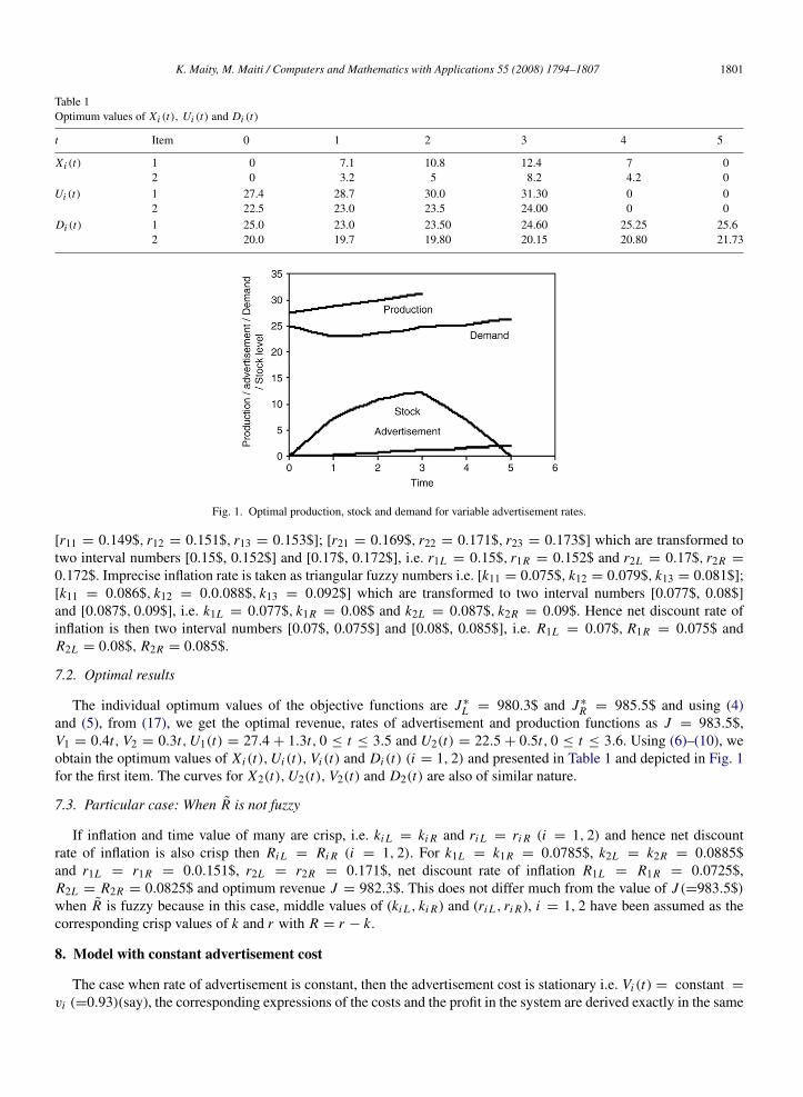
Fig. 1. Optimal production, stock and demand for variable advertisement rates.

[r11 = 0.149$, r12 = 0.151$, r13 = 0.153$]; [r21 = 0.169$, r22 = 0.171$, r23 = 0.173$] which are transformed totwo interval numbers [0.15$, 0.152$] and [0.17$, 0.172$], i.e. r1L = 0.15$, r1R = 0.152$ and r2L = 0.17$, r2R =

0.172$. Imprecise inflation rate is taken as triangular fuzzy numbers i.e. [k11 = 0.075$, k12 = 0.079$, k13 = 0.081$];[k11 = 0.086$, k12 = 0.0.088$, k13 = 0.092$] which are transformed to two interval numbers [0.077$, 0.08$]and [0.087$, 0.09$], i.e. k1L = 0.077$, k1R = 0.08$ and k2L = 0.087$, k2R = 0.09$. Hence net discount rate ofinflation is then two interval numbers [0.07$, 0.075$] and [0.08$, 0.085$], i.e. R1L = 0.07$, R1R = 0.075$ andR2L = 0.08$, R2R = 0.085$.

7.2. Optimal results

The individual optimum values of the objective functions are J ∗

L = 980.3$ and J ∗

R = 985.5$ and using (4)and (5), from (17), we get the optimal revenue, rates of advertisement and production functions as J = 983.5$,V1 = 0.4t, V2 = 0.3t, U1(t) = 27.4 + 1.3t, 0 ≤ t ≤ 3.5 and U2(t) = 22.5 + 0.5t, 0 ≤ t ≤ 3.6. Using (6)–(10), weobtain the optimum values of X i (t), Ui (t), Vi (t) and Di (t) (i = 1, 2) and presented in Table 1 and depicted in Fig. 1for the first item. The curves for X2(t), U2(t), V2(t) and D2(t) are also of similar nature.

7.3. Particular case: When R is not fuzzy

If inflation and time value of many are crisp, i.e. ki L = ki R and ri L = ri R (i = 1, 2) and hence net discountrate of inflation is also crisp then Ri L = Ri R (i = 1, 2). For k1L = k1R = 0.0785$, k2L = k2R = 0.0885$and r1L = r1R = 0.0.151$, r2L = r2R = 0.171$, net discount rate of inflation R1L = R1R = 0.0725$,R2L = R2R = 0.0825$ and optimum revenue J = 982.3$. This does not differ much from the value of J (=983.5$)

when R is fuzzy because in this case, middle values of (ki L , ki R) and (ri L , ri R), i = 1, 2 have been assumed as thecorresponding crisp values of k and r with R = r − k.

8. Model with constant advertisement cost

The case when rate of advertisement is constant, then the advertisement cost is stationary i.e. Vi (t) = constant =

vi (=0.93)(say), the corresponding expressions of the costs and the profit in the system are derived exactly in the same


Table 2Optimum values of Xi (t), Ui (t) and Di (t)

t Item 0 1 2 2.9 4 5

Xi (t) 1 0 7.0 10.3 11.8 6.1 02 0 3.1 4.9 8.0 4.1 0

Ui (t) 1 27.3 28.4 29.6 30.10 0 02 22.4 22.8 23.2 23.70 0 0

Di (t) 1 25.0 23.0 23.50 23.30 23.05 22.82 20.0 19.7 19.40 29.15 18.80 18.53

way as done in the previous sections. These are

Di (t) = Di (0)e−βi t+ vi

(1 − e−βi t

βi

)in (0, T ) (19)

=vi

βi+

(Di (0) −

vi

βi

)e−βi t in (0, T ). (20)

Using (18), (19), (7) and (8), from (1), we get

X i (t) = ui20

(1 − e−αi t

αi

)+ ui1

(t

αi−

1 − e−αi t

α2i

)− Di2

(e−βi t

− e−αi t

αi − βi

), (0, ti ) (21)

= −vi2

(eαi (T −t)

− 1

α2i

)+ Di2

(eαi (T −t)−βi T

− e−βi t

αi − βi

), (ti , T ) (22)

where ui20 = (ui0 −viβi

), Di2 = Di (0) −viβi

and vi2 =viβi

and ti satisfy the continuity condition of X i (t) of Eqs. (20)and (21) at ti .

In this case, we have,

JL(u) =

n∑i=1

(ssi1L − Hi1L − vvi1L − uui1L) (cf. Appendix B)

and

JR(u) =

n∑i=1

(ssi1R − Hi1R − vvi1R − uui1R) (cf. Appendix B)

subject to (4) and

n∑i=1

(Cui0

(ui0ti + ui1

t2i

2

)+ Cui1ti + ci (e

vi − 1)ti

), (γi = 1).

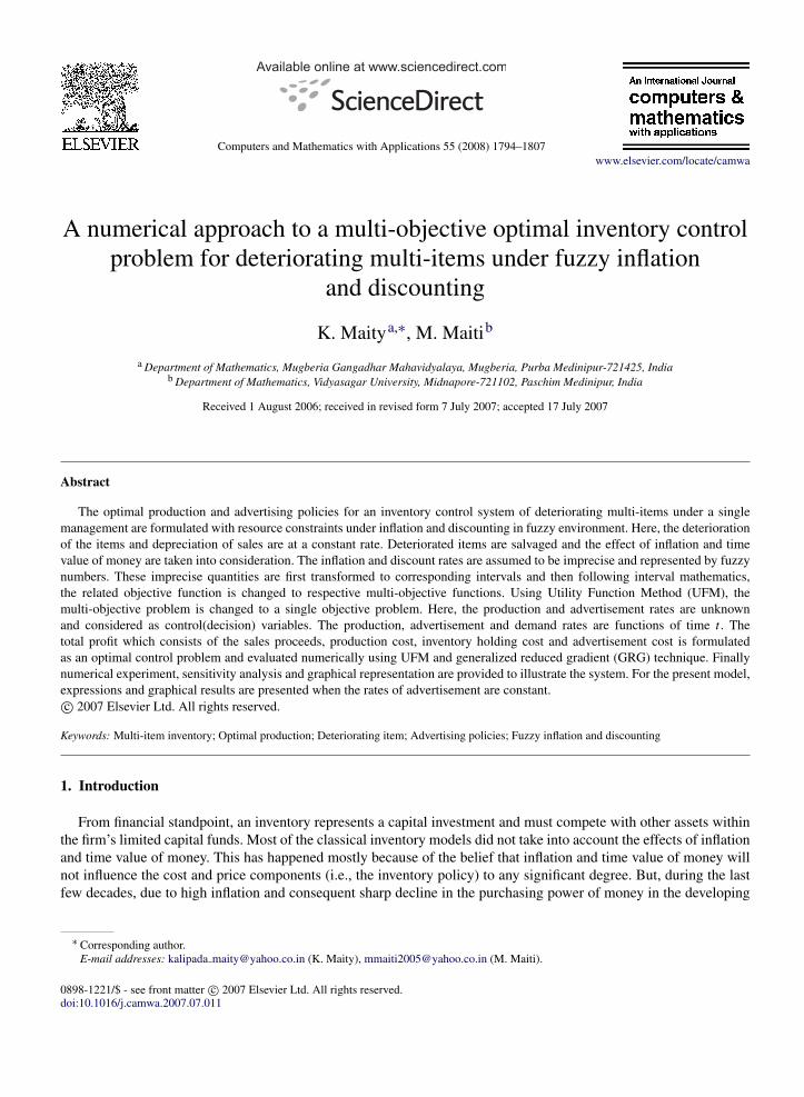
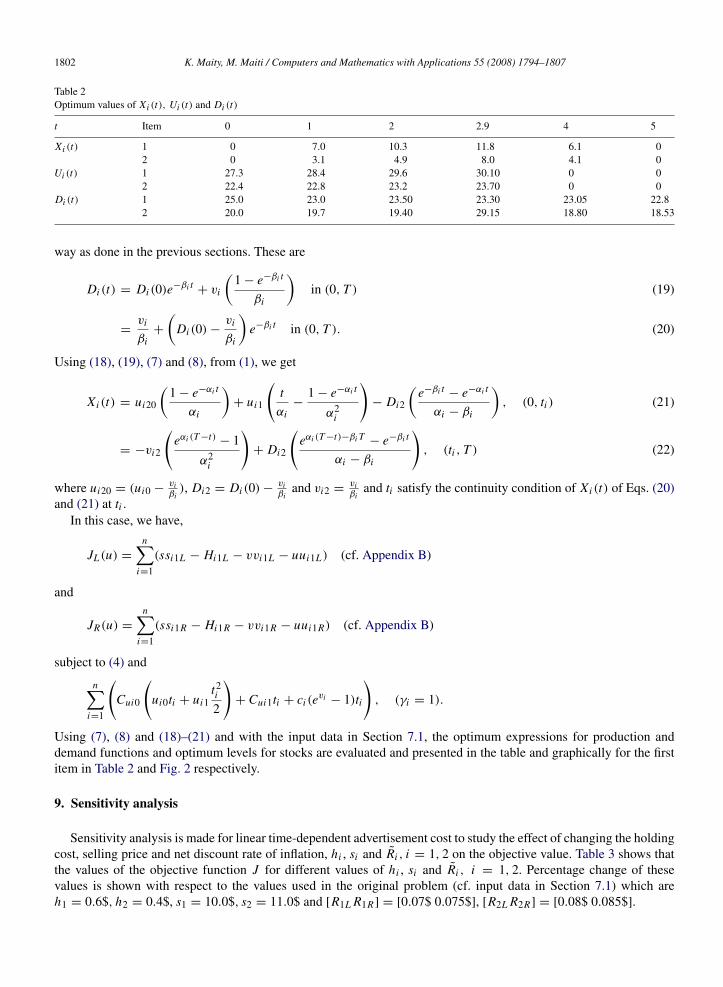
Using (7), (8) and (18)–(21) and with the input data in Section 7.1, the optimum expressions for production anddemand functions and optimum levels for stocks are evaluated and presented in the table and graphically for the firstitem in Table 2 and Fig. 2 respectively.

9. Sensitivity analysis

Sensitivity analysis is made for linear time-dependent advertisement cost to study the effect of changing the holdingcost, selling price and net discount rate of inflation, hi , si and Ri , i = 1, 2 on the objective value. Table 3 shows thatthe values of the objective function J for different values of hi , si and Ri , i = 1, 2. Percentage change of thesevalues is shown with respect to the values used in the original problem (cf. input data in Section 7.1) which areh1 = 0.6$, h2 = 0.4$, s1 = 10.0$, s2 = 11.0$ and [R1L R1R] = [0.07$ 0.075$], [R2L R2R] = [0.08$ 0.085$].


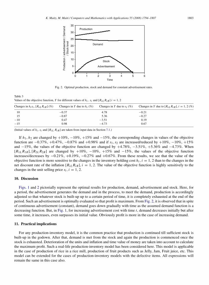
Fig. 2. Optimal production, stock and demand for constant advertisement rates.

Table 3Values of the objective function, Y for different values of hi , si and [Ri L Ri R ] i = 1, 2

Changes in hi si , [Ri L Ri R ] (%) Changes in Y due to hi (%) Changes in Y due to si (%) Changes in Y due to [Ri L Ri R ], i = 1, 2 (%)

10 −0.37 4.78 −0.2115 −0.87 5.36 −0.27

−10 0.47 −3.51 0.19−15 0.98 −4.73 0.67

(Initial values of hi , si and [Ri L Ri R ] are taken from input data in Section 7.1.)

If h1, h2 are changed by +10%, −10%, +15% and −15%, the corresponding changes in values of the objectivefunction are −0.37%, +0.47%, −0.87% and +0.98% and if s1, s2 are increased/reduced by +10%, −10%, +15%and −15%, the values of the objective function are changed by +4.78%, −3.51%, +5.36% and −4.73%. When[R1L R1R], [R2L R2R] are changed by +10%, −10%, +15% and −15%, the values of the objective functionincreases/decreases by −0.21%, +0.19%, −0.27% and +0.67%. From these results, we see that the value of theobjective function is more sensitive to the changes in the inventory holding cost hi , i = 1, 2 than to the changes in thenet discount rate of the inflation [Ri L Ri R], i = 1, 2. The value of the objective function is highly sensitively to thechanges in the unit selling price si , i = 1, 2.

10. Discussion

Figs. 1 and 2 pictorially represent the optimal results for production, demand, advertisement and stock. Here, fora period, the advertisement generates the demand and in the process, to meet the demand, production is accordinglyadjusted so that whatever stock is built-up up to a certain period of time, it is completely exhausted at the end of theperiod. Such an advertisement is optimally evaluated so that profit is maximum. From Fig. 2, it is observed that in spiteof continuous advertisement (constant), demand goes down gradually with time as the assumed demand function is adecreasing function. But, in Fig. 1, for increasing advertisement cost with time t , demand decreases initially but aftersome time, it increases, even surpasses its initial value. Obviously profit is more in the case of increasing demand.

11. Practical implications

For any production-inventory model, it is the common practice that production is continued till sufficient stock isbuilt-up in the godown. After that, demand is met from the stock and again the production is commenced once thestock is exhausted. Deterioration of the units and inflation and time value of money are taken into account to calculatethe maximum profit. Such a real-life production-inventory model has been considered here. This model is applicablein the case of production of rice in a rice mill, production of fruit products such as Jelly, Jam, Fruit juice, etc. Thismodel can be extended for the cases of production-inventory models with the defective items. All expressions willremain the same in this case also.


12. Conclusion

The present paper deals with the optimum production and advertising policy for a multi-item production-inventory system with deteriorating units, depreciation rate of sales, salvage value of deteriorated items, spacecapacity constraint, investment constraint and dynamic demand under the imprecise inflation and time discountingenvironment. Also some ideas such as (i) optimal control production problem for deteriorating multi-items, (ii)advertisement-dependent demand, (iii) dynamic production function, (iv) production-quantity-dependent unit costand (v) imprecise inflation and imprecise depreciation in many value have been introduced for the first time.

In the solution approach, the new ideas are: (i) using interval mathematics for fuzzy numbers for their crisp value.In this connection, the Lemma 1 with an interval power of exponential has been reduced to an interval for the firsttime. As already mentioned earlier, for the first time, a new type of utility function with individual optimum valueshas been defined and used to convert multi-objective problem to a single objective one in an inventory control system.The formulation and analysis presented here can be extended to other production-inventory problems with differenttypes of demand, advertisement, deterioration, defect, price discount, etc.

Appendix A

For simplicity, we take γ1 = 1 = γ2.

Hi1L = ui10

(1 − e−Ri R ti

Ri Rαi−

1 − e−(Ri R+αi )ti

αi (Ri R + αi )

)+

(ui1 −

vi

βi

)(−ti e−Ri R ti

Ri Rβi+

1 − e−Ri R ti

R2i Rβi

−1 − e−Ri R ti

α2i Ri R

+1 − e−(Ri R+αi )ti

(Ri R + αi )α2i

)−

(Di (0) +

vi

β2i

)(1 − e−(Ri R+βi )ti

(Ri R + βi )(αi − βi )−


(αi − βi )(Ri R + αi )

), (23)

Hi1R = ui10

(1 − e−Ri L ti

Ri Lαi−

1 − e−(Ri L+αi )ti

αi (Ri L + αi )

)+

(ui1 −

vi

βi

)(−ti e−Ri L ti

Ri Lβi+

1 − e−Ri L ti

R2i Lβi

−1 − e−Ri L ti

α2i Ri L

+1 − e−(Ri L+αi )ti

(Ri L + αi )α2i

)−

(Di (0) +

vi

β2i

)(1 − e−(Ri L+βi )ti

(Ri L + βi )(αi − βi )−


(αi − βi )(Ri L + αi )

), (24)

Hi2L =vi

βi

(T eαi T

(e−(Ri R+αi )ti − e−(Ri R+αi )T

(Ri R + αi )αi

)+ T

(e−Ri R T

− e−Ri R ti

Ri R

)+

(e−Ri R T

− e−Ri R ti

R2i R

))

−vi

βi

((e−Ri R T

− eαi T −(Ri R+αi )ti

(Ri R + αi )α2i

)+

eRi R T− e−Ri R ti

Ri Rα2i

)

−vi

β2i

(eαi T −(αi +Ri R)ti1 − e−Ri R T

αi (αi + Ri R)−

e−Ri R ti1 − e−Ri R T

αi Ri R

)

+

(Di (0) +

vi

β2i

)(e(αi −βi )T −(αi +Ri R)ti1 − e−(Ri R+βi )T

(αi − βi )(αi + Ri R)−

e−(βi +Ri R)ti1 − e−(βi +Ri R)T

(αi − βi )(αi + Ri R)

), (25)

Hi2R =vi

βi

(T eαi T

(e−(Ri L+αi )ti − e−(Ri L+αi )T

(Ri L + αi )αi

)+ T

(e−Ri L T

− e−Ri L ti

Ri L

)+

(e−Ri L T

− e−Ri L ti

R2i L

))

−vi

βi

((e−Ri L T

− eαi T −(Ri L+αi )ti

(Ri L + αi )α2i

)+

eRi L T− e−Ri L ti

Ri Lα2i

)

−vi

β2i

(eαi T −(αi +Ri L )ti1 − e−Ri L T

αi (αi + Ri L)−

e−Ri L ti1 − e−Ri L T

αi Ri L

)

+

(Di (0) +

vi

β2i

)(e(αi −βi )T −(αi +Ri L )ti1 − e−(Ri L+βi )T

(αi − βi )(αi + Ri L)−

e−(βi +Ri L )ti1 − e−(βi +Ri L )T

(αi − βi )(αi + Ri L)

), (26)


ssi L = sivi

βi

(1 − e−Ri R T

R2i R

−T e−Ri R

Ri R

)− sivi

(1 − eRi R T

β2i Ri R

)+ Di1(0)

(1 − e(βi +Ri R)T

Ri R + βi

), (27)

ssi R = sivi

βi

(1 − e−Ri L T

R2i L

−T e−Ri L

Ri L

)− sivi

(1 − eRi L T

β2i Ri L

)+ Di1(0)

(1 − e(βi +Ri L )T

Ri L + βi

), (28)

Hi L = (hi − biαi )(Hi1L + Hi2L), (29)

Hi R = (hi − biαi )(Hi1R + Hi2R), (30)

vvi L = ci

(e(vi −Ri R)T

− 1vi − Ri R

−1 − e−Ri R T

Ri R

), (31)

vvi R = ci

(e(vi −Ri L )T

− 1vi − Ri L

−1 − e−Ri L T

Ri L

), (32)

uui L = (Cui0ui0 + Cui1)

(1 − e−Ri R ti

Ri R

)+ Cui0u11

(1 − (1 + ti Ri R)e−Ri R ti

R2i R

), (33)

and

uui R = (Cui0ui0 + Cui1)

(1 − e−Ri L ti

Ri L

)+ Cui0u11

(1 − (1 + ti Ri L)e−Ri L ti

R2i L

)(34)

where Di1(0) = si (Di (0) +viβ2

i).

Appendix B

For simplicity, we take γ1 = 1 = γ2.

Hi11L = ui20

(1 − e−Ri R ti

Ri Rαi−


αi (Ri R + αi )

)+ ui1

(−ti e−Ri R ti

Ri Rβi+

1 − e−Ri R ti

R2i Rβi

−1 − e−Ri R ti

α2i Ri R

+1 − e−(Ri R+αi )ti

(Ri R + αi )α2i

)−

(Di (0) −

vi

βi

)(1 − e−(Ri R+βi )ti

(Ri R + βi )(αi − βi )−


(αi − βi )(Ri R + αi )

), (35)

Hi11R = ui20

(1 − e−Ri L ti

Ri Lαi−


αi (Ri L + αi )

)+

(ui1 −

vi

βi

)(−ti e−Ri L ti

Ri Lβi+

1 − e−Ri L ti

R2i Lβi

−1 − e−Ri L ti

α2i Ri L

+1 − e−(Ri L+αi )ti

(Ri L + αi )α2i

)−

(Di (0) −

vi

βi

)(1 − e−(Ri L+βi )ti

(Ri L + βi )(αi − βi )−


(αi − βi )(Ri L + αi )

), (36)

Hi21L =vi

βi

(eαi T −(αi +Ri R)ti1 − e−Ri R T

αi (αi + Ri R)−

e−Ri R ti1 − e−Ri R T

αi Ri R

)

+

(Di (0) −

vi

βi

)(e(αi −βi )T −(αi +Ri R)ti1 − e−(Ri R+βi )T

(αi − βi )(αi + Ri R)−

e−(βi +Ri R)ti1 − e−(βi +Ri R)T

(αi − βi )(αi + Ri R)

), (37)

Hi21R =vi

βi

(eαi T −(αi +Ri L )ti1 − e−Ri L T

αi (αi + Ri L)−

e−Ri L ti1 − e−Ri L T

αi Ri L

)

+

(Di (0) −

vi

βi

)(e(αi −βi )T −(αi +Ri L )ti1 − e−(Ri L+βi )T

(αi − βi )(αi + Ri L)−

e−(βi +Ri L )ti1 − e−(βi +Ri L )T

(αi − βi )(αi + Ri L)

), (38)


ssi1L = si

(vi

(1 − eRi R T

βi Ri R

)+

(Di (0) −

vi

βi

)(1 − e(βi +Ri R)T

Ri R + βi

)), (39)

ssi1R = si

(vi

(1 − eRi L T

βi Ri L

)+

(Di (0) −

vi

βi

)(1 − e(βi +Ri L )T

Ri L + βi

)), (40)

Hi1L = (hi − biαi )(Hi11L + Hi21L), (41)

Hi1R = (hi − biαi )(Hi11R + Hi21R), (42)

vvi1L = ci (evi − 1)

(1 − e−Ri R T

Ri R

), (43)

vvi1L = ci (evi − 1)

(1 − e−Ri L T

Ri R

), (44)

uui1L = (Cui0ui0 + Cui1)

(1 − e−Ri R ti

Ri R

)+ u11

(1 − (1 + ti Ri R)e−Ri R ti

R2i R

), (45)

and

uui1R = (Cui0ui0 + Cui1)

(1 − e−Ri L ti

Ri L

)+ Cui0u11

(1 − (1 + ti Ri L)e−Ri L ti

R2i L

). (46)

References

[1] J.A. Buzacott, Economic order quantities with inflation, Operational Research Quarterly 26 (1975) 553–558.[2] R.B. Misra, A note on optimal inventory management under inflation, Naval Research Logistics 26 (1979) 161–165.[3] S.T. Lo, H.M. Wee, W.C. Huang, An integrated production-inventory model with imperfect production process and weibull distribution

deterioration under inflation, International Journal of Production Research 106 (2007) 248–260.[4] H.J. Chang, C.Y. Dye, An EOQ model for deteriorating items with time-varying demand and partial backlogging, Journal of Operational

Research Society 50 (1999) 1176–1182.[5] S. Papachristos, K. Skouri, An inventory model of deteriorating items, quantity discount, pricing and time-dependent partial backlogging,

International Journal of Production Economics 83 (2003) 247–256.[6] K. Maity, M. Maiti, Possibility and necessity constraints and their defuzzification — a multi-item production-inventory scenario via optimal

control theory, European Journal of Operational Research 177 (2007) 882–896.[7] S.K. Goyal, B.C. Giri, Recent trends modelling of deteriorating inventory, European Journal of Operational Research 134 (2001) 1–16.[8] I.D. Cho, Analysis of optimal production and advertising policies, International Journal of Systems Science 27 (1996) 1297–1305.[9] T.K. Datta, K. Paul, A.K. Pal, Demand promotion by up gradation under stock dependent demand situation-a model, International Journal of

Production Economics 55 (1998) 31–38.[10] M. Mandal, M. Maiti, Inventory model for damageable items with stock dependent demand and shortages, Opsearch 34 (1997) 155–166.[11] M. Khouja, The economical production lot size model under volume flexibility, Computer and Operations Research 22 (1995) 515–525.[12] R.M. Bhandari, P.K. Sharma, The economic production lot size model with variable cost function, Opsearch 36 (1999) 137–150.[13] J.Q. Hu, R. Loulou, Multi-product production/inventory control under random demands, IEEE Transactions on Automatic Control 40 (1995)

350–355.[14] B.M. Worell, M.A. Hall, The analysis of inventory control model using polynomial geometric programming, International Journal of

Production Research 20 (1982) 657–667.[15] M.J. Chandra, M.L. Bahner, The effects of inflation and time value of money on some inventory systems, International Journal of Production

Research 23 (1985) 723–730.[16] K. Maity, M. Maiti, Production inventory system for deteriorating multi-item with inventory-dependent dynamic demands under inflation and

discounting, Tamsui Oxford Journal of Management Science 21 (2005) 1–18.[17] L.A. Zadeh, Fuzzy sets, Information and Control 8 (1965) 338–356.[18] R.E. Bellman, L.A. Zadeh, Decision making in a fuzzy environment, Management Science 17 (1970) B141–B164.[19] H.J. Zimmermann, Description and optimization of fuzzy system, International Journal of General Systems 2 (1985) 209–215.[20] T.K. Roy, M. Maiti, A multi-item fuzzy displayed inventory model under limited shelf-space, The International Journal of Fuzzy Mathematics

8 (2000) 881–888.[21] N.K. Mahapatra, M. Maiti, Decision process for multi-objective, multi-item production-inventory system via interactive fuzzy satisficing

technique, Computers and Mathematics with Applications 49 (2005) 805–821.[22] J.S. Yao, K. Wu, Consumer surplus and producer surplus for fuzzy demand and fuzzy supply, Fuzzy Sets and Systems 103 (1999) 421–426.


[23] J.K. Dey, S. Kar, M. Maiti, An interactive method for inventory control with fuzzy lead-time and dynamic demand, European Journal ofOperational Research 167 (2005) 381–397.

[24] G. Padmanabhan, P. Vrat, Analysis of multi-systems under resource constraint, a nonlinear goal programming approach, Engineering Costand Production Management 13 (1990) 104–112.

[25] T.K. Roy, M. Maiti, Multi-objective inventory models of deteriorating items with some constraints in a fuzzy environment, Computers andOperations Research 25 (1998) 1085–1095.

[26] G.A. Gabriel, K.M. Ragsdell, The generalized reduced gradient method, AMSE Journal of Engineering for Industry 99 (1977) 384–400.[27] R.E. Moore, Interval Analysis, Prentice-Hall, Inc., 1966.[28] K. Maity, M. Maiti, Numerical approach of multi-objective optimal control problem in imprecise environment, Fuzzy Optimization and

Decision Making 4 (2005) 313–330.[29] P. Grzegorzewski, Nearest interval approximation of a fuzzy number, Fuzzy Sets and Systems 130 (2002) 321–330.[30] K.M. Miettinen, Non-Linear Multi-Objective, Optimization, Kluwer’s International Series, 1999.

Documents

A numerical approach to a multi-objective optimal ... · In the case of multi-item inventory models, it is possible to study each item separately as long as there is no interactions