Embed Size (px)
Citation preview
A NOVEL SPECTRAL APPROXIMATION FORTHE TWO-DIMENSIONAL FRACTIONAL SUB-DIFFUSION PROBLEMS
A.H. BHRAWY1,2, M.A. ZAKY3, D. BALEANU4,5, M.A. ABDELKAWY2
1Department of Mathematics, Faculty of Science, King Abdulaziz University, Jeddah, Saudi ArabiaE-mail: [email protected]
2Department of Mathematics, Faculty of Science, Beni-Suef University, Beni-Suef, EgyptE-mail: [email protected]
3Department of Applied Mathematics, National Research Center, Cairo, EgyptE-mail: [email protected]
4Cankaya University, Faculty of Art and Sciences,Department of Mathematics and Computer Sciences, Balgat 0630, Ankara, Turkey
5Institute of Space Sciences,P.O.BOX, MG-23, RO 077125, Magurele-Bucharest, Romania
E-mail: [email protected]
Received November 3, 2014
This paper reports a new numerical method that enables easy and convenientdiscretization of a two-dimensional sub-diffusion equation with fractional derivativesof any order. The suggested method is based on Jacobi tau spectral procedure togetherwith the Jacobi operational matrix for fractional derivatives, described in the Caputosense. Such approach has the advantage of reducing the problem to the solution of asystem of algebraic equations, which may then be solved by any standard numericaltechnique. The validity and effectiveness of the method are demonstrated by solvingtwo numerical examples, which are presented in the form of tables and graphs to makemore easier comparisons with the exact solutions and the results obtained by othermethods.
Key words: Two-dimensional fractional diffusion equations; Tau method;Shifted Jacobi polynomials; Operational matrix; Caputo derivative.
PACS: 03.65.Db,02.30.Hq.
1. INTRODUCTION
Fractional calculus goes back to the beginning of the theory of differential cal-culus and deals with the generalization of standard integrals and derivatives to anarbitrary real-valued order [1–3]. This subject is one of the most interdisciplinaryfields of mathematics and has gained considerable popularity and importance due toits attractive applications as a new modeling tool in a variety of scientific and en-gineering fields, such as viscoelastic systems [4], transport phenomena [5], control[6], market dynamics [7], fractional kinetics [8], pharmacokinetics [9], advection-dispersion systems in earth science [10], and tumor growth [11]. Modeling successesfor these phenomena have recently been reported using fractional derivatives for both
RJP 60(Nos. 3-4), 344–359 (2015) (c) 2015 - v.1.3a*2015.4.21Rom. Journ. Phys., Vol. 60, Nos. 3-4, P. 344–359, Bucharest, 2015
2 Novel spectral approximation for two-dimensional fractional sub-diffusion problems 345
ordinary and partial differential equations. In particular, it has been reported that cer-tain kinds of dynamic natural phenomena, such as nonlocal diffusion modeled infractal dimensions, cannot be properly described in terms of traditional integer orderdifferential equations [3, 12, 13]. Fractional diffusion equation is a class of importantfractional partial differential equations, which has been widely applied in modelingof anomalous diffusive systems, unification of diffusion and wave propagation phe-nomenon, description of fractional random walk, etc. [14, 15]. Fractional kineticequations have proved particularly useful in the context of anomalous sub-diffusion[16]. For recent articles for solving various versions of such equations, see Refs.[17–22].
Fractional sub-diffusion equation is a subclass of anomalous diffusive systems,which is obtained by replacing the time derivative in ordinary diffusion by a fractionalderivative of order ν with 0< ν < 1. The mean square displacement of the particlesfrom the original starting site is no longer linear in time but verifies a generalizedFick’s second law. Sub-diffusive motion is characterized by an asymptotic long timebehavior of the mean square displacement of the form⟨
x2(t)⟩∼
2Kν
Γ(1+ν)tν , t→∞,
where ν (0< ν < 1) is the anomalous diffusion exponent and Kν is the generalizeddiffusion coefficient. It turns out that the probability density function u(x, t) thatdescribes anomalous sub-diffusive particle follows the fractional diffusion equation[16, 23]:
ut = 0D1−νt ∆u, t > 0,
where ∆ is the Laplacian and 0D1−νt denotes the Caputo fractional derivative opera-
tor.Several numerical methods have been proposed in the last few years for solv-
ing such equation. In Refs. ([24]-[33]), the researchers developed finite differencemethod. Particularly, Cui [29] and Gao et al. [31] concentrated on the compactdifference schemes for promoting the spatial accuracy. Zhuang et al. [32] pro-posed explicit and implicit Euler approximations for the variable-order fractionaladvection-diffusion equation with a nonlinear source term and they discussed an im-plicit numerical method for the nonlinear fractional reaction sub-diffusion process inRef. [34]. Zhang and Sun [35] used alternating direction implicit (ADI) schemes fora two-dimensional time-fractional sub-diffusion equation. Lin and Xu [36] proposeda finite difference method in the time direction and a Legendre spectral method in thespace direction for the time-fractional diffusion equation. Li and Xu [37] extendedtheir previous work and proposed a spectral method in both temporal and spatial dis-cretizations for a time-space fractional partial differential equation based on a weakformulation and a detailed error analysis was carried out. Spectral methods offer
RJP 60(Nos. 3-4), 344–359 (2015) (c) 2015 - v.1.3a*2015.4.21
346 A.H. Bhrawy et al. 3
spectral accuracy, meaning that the error decreases exponentially fast as the numberof degrees of freedom increases. However, the application of spectral methods toirregular domains is not straightforward. Spectral methods have emerged as compet-itive alternatives to these methods [37–41].
In this paper, our main goal is to propose a new spectral algorithm in bothtemporal and spatial discretizations to provide an accurate numerical solution of thetwo-dimensional fractional sub-diffusion equations. This algorithm is based princi-pally on shifted Jacobi tau spectral method combined with the generalized shiftedJacobi operational matrix of derivatives. To the best of our knowledge, there are noresults on the spectral tau method for solving the two-dimensional time- or space-fractional partial differential equations.
The outline of this article is as follows: In Section 2, we present some frac-tional calculus preliminaries. In Section 3, the shifted Jacobi polynomials with theirproperties and their operational matrix to fractional differentiation are presented. InSection 4, by using tau spectral method, we construct and develop an algorithm forthe solution of the two-dimensional fractional sub-diffusion equations with Dirichletconditions. The accuracy and efficiency of of the proposed spectral algorithm are in-vestigated with two illustrative numerical experiments in Section 5. The last sectionconsists of some obtained conclusions.
2. FRACTIONAL DERIVATIVES
A complication associated with fractional derivatives is that there are severaldefinitions of exactly what a fractional derivative means [3]. The two most commonlyused definitions are based on Riemann-Liouville and Caputo senses. In order tosimplify the basic definitions we consider the time interval [0, τ ] instead of [a,τ ]and omit a = 0 as an index in the differential operator. If we consider the functionf(t) ∈ Cn[0, τ ], then the Riemann-Liouville definition for fractional derivative isgiven by:
RL0 Dν
t f(t) =
1
Γ(n−ν)dn
dtn
t∫0
f(τ)(t−τ)ν+1−ndτ, n−1< ν < n,
fn(t), ν = n.
(1)
where ν is the order of the derivative. An alternative definition, known as the Caputofractional derivative, is defined as
0Dνt f(t) =
1
Γ(n−ν)
t∫0
f (n)(τ)(t−τ)ν+1−ndτ, n−1< ν < n,
fn(t), ν = n.
(2)
RJP 60(Nos. 3-4), 344–359 (2015) (c) 2015 - v.1.3a*2015.4.21
4 Novel spectral approximation for two-dimensional fractional sub-diffusion problems 347
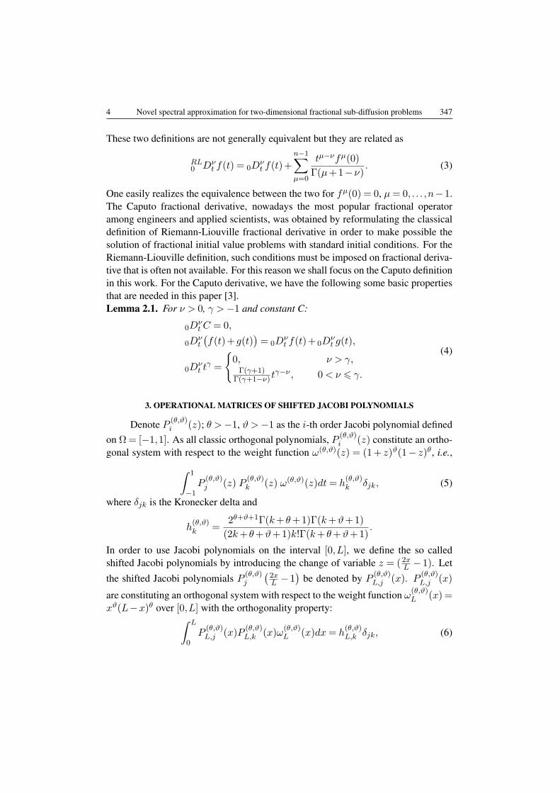
These two definitions are not generally equivalent but they are related as
RL0 Dν
t f(t) = 0Dνt f(t)+
n−1∑µ=0
tµ−νfµ(0)
Γ(µ+1−ν). (3)
One easily realizes the equivalence between the two for fµ(0) = 0, µ= 0, . . . ,n−1.The Caputo fractional derivative, nowadays the most popular fractional operatoramong engineers and applied scientists, was obtained by reformulating the classicaldefinition of Riemann-Liouville fractional derivative in order to make possible thesolution of fractional initial value problems with standard initial conditions. For theRiemann-Liouville definition, such conditions must be imposed on fractional deriva-tive that is often not available. For this reason we shall focus on the Caputo definitionin this work. For the Caputo derivative, we have the following some basic propertiesthat are needed in this paper [3].Lemma 2.1. For ν > 0, γ >−1 and constant C:
0Dνt C = 0,
0Dνt
(f(t)+g(t)
)= 0D
νt f(t)+ 0D
νt g(t),
0Dνt t
γ =
0, ν > γ,Γ(γ+1)
Γ(γ+1−ν) tγ−ν , 0< ν ⩽ γ.
(4)
3. OPERATIONAL MATRICES OF SHIFTED JACOBI POLYNOMIALS
Denote P (θ,ϑ)i (z); θ >−1, ϑ >−1 as the i-th order Jacobi polynomial defined
on Ω= [−1,1]. As all classic orthogonal polynomials, P (θ,ϑ)i (z) constitute an ortho-
gonal system with respect to the weight function ω(θ,ϑ)(z) = (1+ z)ϑ(1− z)θ, i.e.,∫ 1
−1P
(θ,ϑ)j (z) P
(θ,ϑ)k (z) ω(θ,ϑ)(z)dt= h
(θ,ϑ)k δjk, (5)
where δjk is the Kronecker delta and
h(θ,ϑ)k =
2θ+ϑ+1Γ(k+θ+1)Γ(k+ϑ+1)
(2k+θ+ϑ+1)k!Γ(k+θ+ϑ+1).
In order to use Jacobi polynomials on the interval [0,L], we define the so calledshifted Jacobi polynomials by introducing the change of variable z = (2xL − 1). Let
the shifted Jacobi polynomials P(θ,ϑ)j
(2xL −1
)be denoted by P
(θ,ϑ)L,j (x). P
(θ,ϑ)L,j (x)
are constituting an orthogonal system with respect to the weight function ω(θ,ϑ)L (x) =
xϑ(L−x)θ over [0,L] with the orthogonality property:∫ L
0P
(θ,ϑ)L,j (x)P
(θ,ϑ)L,k (x)ω
(θ,ϑ)L (x)dx= h
(θ,ϑ)L,k δjk, (6)
RJP 60(Nos. 3-4), 344–359 (2015) (c) 2015 - v.1.3a*2015.4.21
348 A.H. Bhrawy et al. 5
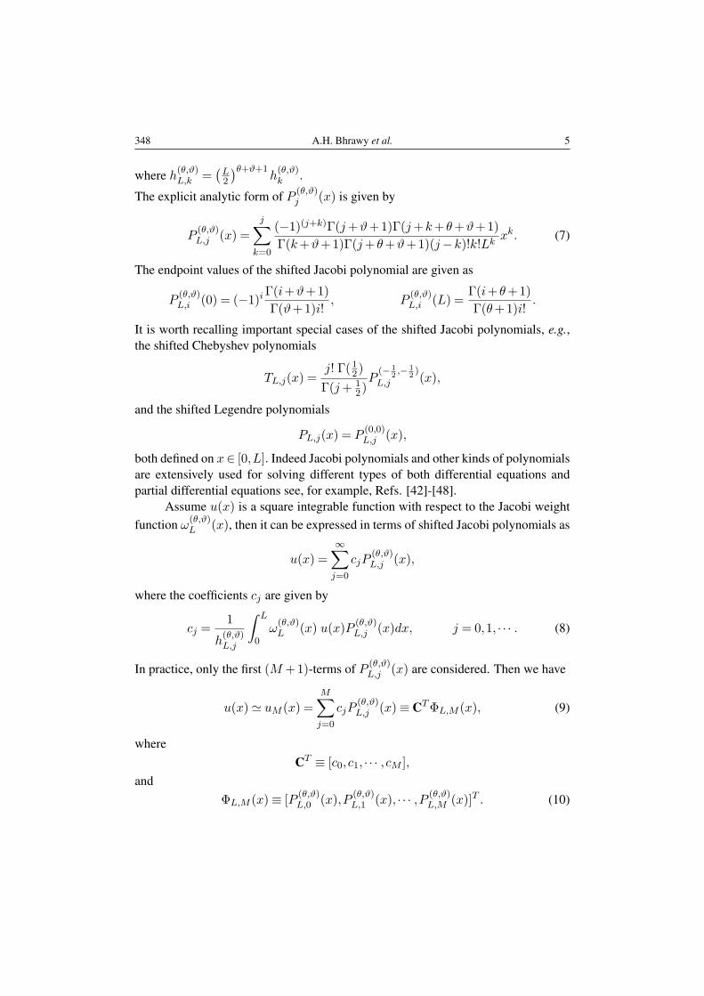
where h(θ,ϑ)L,k =
(L2
)θ+ϑ+1h(θ,ϑ)k .
The explicit analytic form of P (θ,ϑ)j (x) is given by
P(θ,ϑ)L,j (x) =
j∑k=0
(−1)(j+k)Γ(j+ϑ+1)Γ(j+k+θ+ϑ+1)
Γ(k+ϑ+1)Γ(j+θ+ϑ+1)(j−k)!k!Lkxk. (7)
The endpoint values of the shifted Jacobi polynomial are given as
P(θ,ϑ)L,i (0) = (−1)i
Γ(i+ϑ+1)
Γ(ϑ+1)i!, P
(θ,ϑ)L,i (L) =
Γ(i+θ+1)
Γ(θ+1)i!.
It is worth recalling important special cases of the shifted Jacobi polynomials, e.g.,the shifted Chebyshev polynomials
TL,j(x) =j! Γ(12)
Γ(j+ 12)P
(− 12,− 1
2)
L,j (x),
and the shifted Legendre polynomials
PL,j(x) = P(0,0)L,j (x),
both defined on x∈ [0,L]. Indeed Jacobi polynomials and other kinds of polynomialsare extensively used for solving different types of both differential equations andpartial differential equations see, for example, Refs. [42]-[48].
Assume u(x) is a square integrable function with respect to the Jacobi weightfunction ω
(θ,ϑ)L (x), then it can be expressed in terms of shifted Jacobi polynomials as
u(x) =
∞∑j=0
cjP(θ,ϑ)L,j (x),
where the coefficients cj are given by
cj =1
h(θ,ϑ)L,j
∫ L
0ω(θ,ϑ)L (x) u(x)P
(θ,ϑ)L,j (x)dx, j = 0,1, · · · . (8)
In practice, only the first (M +1)-terms of P (θ,ϑ)L,j (x) are considered. Then we have
u(x)≃ uM (x) =
M∑j=0
cjP(θ,ϑ)L,j (x)≡ CTΦL,M (x), (9)
whereCT ≡ [c0, c1, · · · , cM ],
andΦL,M (x)≡ [P
(θ,ϑ)L,0 (x),P
(θ,ϑ)L,1 (x), · · · ,P (θ,ϑ)
L,M (x)]T . (10)
RJP 60(Nos. 3-4), 344–359 (2015) (c) 2015 - v.1.3a*2015.4.21
6 Novel spectral approximation for two-dimensional fractional sub-diffusion problems 349
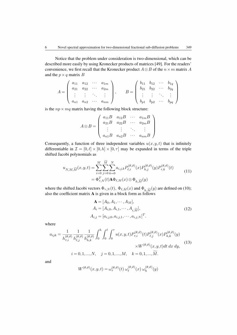
Notice that the problem under consideration is two-dimensional, which can bedescribed more easily by using Kronecker products of matrices [49]. For the readers’convenience, we first recall that the Kronecker product A⊗B of the n×m matrix Aand the p× q matrix B
A=
a11 a12 · · · a1ma21 a22 · · · a2m
......
. . ....
an1 an2 · · · anm
, B =
b11 b12 · · · b1qb21 b22 · · · b2q
......
. . ....
bp1 bp2 · · · bpq
is the np×mq matrix having the following block structure:
A⊗B =
a11B a12B · · · a1mBa21B a22B · · · a2mB
......
. . ....
an1B an2B · · · anmB
Consequently, a function of three independent variables u(x,y, t) that is infinitelydifferentiable in I = [0, ℓ]× [0,h]× [0, τ ] may be expanded in terms of the tripleshifted Jacobi polynomials as
uN,M,M
(x,y, t) =M∑i=0
M∑j=0
N∑k=0
ai,j,kP(θ,ϑ)ℓ,i (x)P
(θ,ϑ)h,j (y)P
(θ,ϑ)τ,k (t)
= ΦTτ,N (t)AΦℓ,M (x)⊗Φ
h,M(y)
(11)
where the shifted Jacobi vectors Φτ,N (t), Φℓ,M (x) and Φh,M
(y) are defined on (10);also the coefficient matrix A is given in a block form as follows
A = [A0,A1, · · · ,AM ],
Ai = [Ai,0,Ai,1, · · · ,Ai,M],
Ai,j = [ai,j,0,ai,j,1, · · · ,ai,j,N ]T .
(12)
where
aijk =1
h(θ,ϑ)τ,i
1
h(θ,ϑ)ℓ,j
1
h(θ,ϑ)h,k
∫ h
0
∫ ℓ
0
∫ τ
0u(x,y, t)P
(θ,ϑ)τ,i (t)P
(θ,ϑ)ℓ,j (x)P
(θ,ϑ)h,k (y)
×W (θ,ϑ)(x,y, t)dt dx dy,
i= 0,1, ...,N, j = 0,1, ...,M, k = 0,1, ...,M .
(13)
and
W (θ,ϑ)(x,y, t) = ω(θ,ϑ)τ (t) ω
(θ,ϑ)ℓ (x) ω
(θ,ϑ)h (y)
RJP 60(Nos. 3-4), 344–359 (2015) (c) 2015 - v.1.3a*2015.4.21
350 A.H. Bhrawy et al. 7
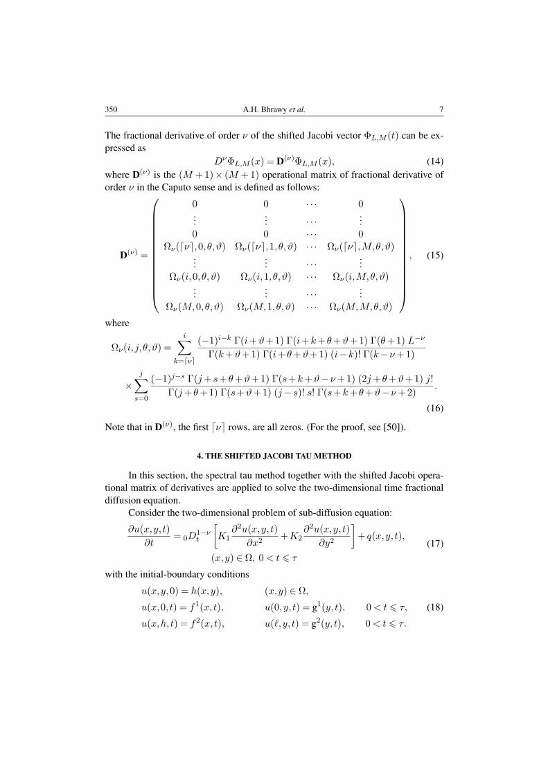
The fractional derivative of order ν of the shifted Jacobi vector ΦL,M (t) can be ex-pressed as
DνΦL,M (x) = D(ν)ΦL,M (x), (14)where D(ν) is the (M +1)× (M +1) operational matrix of fractional derivative oforder ν in the Caputo sense and is defined as follows:
D(ν) =
0 0 · · · 0...
... · · ·...
0 0 · · · 0Ων(⌈ν⌉,0,θ,ϑ) Ων(⌈ν⌉,1,θ,ϑ) · · · Ων(⌈ν⌉,M,θ,ϑ)
...... · · ·
...Ων(i,0,θ,ϑ) Ων(i,1,θ,ϑ) · · · Ων(i,M,θ,ϑ)
...... · · ·
...Ων(M,0,θ,ϑ) Ων(M,1,θ,ϑ) · · · Ων(M,M,θ,ϑ)
, (15)
where
Ων(i, j,θ,ϑ) =
i∑k=⌈ν⌉
(−1)i−k Γ(i+ϑ+1) Γ(i+k+θ+ϑ+1) Γ(θ+1) L−ν
Γ(k+ϑ+1) Γ(i+θ+ϑ+1) (i−k)! Γ(k−ν+1)
×j∑
s=0
(−1)j−s Γ(j+s+θ+ϑ+1) Γ(s+k+ϑ−ν+1) (2j+θ+ϑ+1) j!
Γ(j+θ+1) Γ(s+ϑ+1) (j−s)! s! Γ(s+k+θ+ϑ−ν+2).
(16)
Note that in D(ν), the first ⌈ν⌉ rows, are all zeros. (For the proof, see [50]).
4. THE SHIFTED JACOBI TAU METHOD
In this section, the spectral tau method together with the shifted Jacobi opera-tional matrix of derivatives are applied to solve the two-dimensional time fractionaldiffusion equation.
Consider the two-dimensional problem of sub-diffusion equation:
∂u(x,y, t)
∂t= 0D
1−νt
[K1
∂2u(x,y, t)
∂x2+K2
∂2u(x,y, t)
∂y2
]+ q(x,y, t),
(x,y) ∈ Ω, 0< t⩽ τ
(17)
with the initial-boundary conditions
u(x,y,0) = h(x,y),
u(x,0, t) = f1(x,t),
u(x,h,t) = f2(x,t),
(x,y) ∈ Ω,
u(0,y, t) = g1(y,t), 0< t⩽ τ,
u(ℓ,y, t) = g2(y,t), 0< t⩽ τ.
(18)
RJP 60(Nos. 3-4), 344–359 (2015) (c) 2015 - v.1.3a*2015.4.21
8 Novel spectral approximation for two-dimensional fractional sub-diffusion problems 351
where K1 and K2 are positive constants, and Ω= [0, ℓ]× [0,h] is a finite rectangulardomain. It is worthy to mention here that, since the pure spectral tau method wouldnot use any interpolation operator, we approximated the solution and known func-tions in terms of shifted Jacobi polynomials in order to use orthogonality of suchpolynomials for computing the spectral tau coefficients.
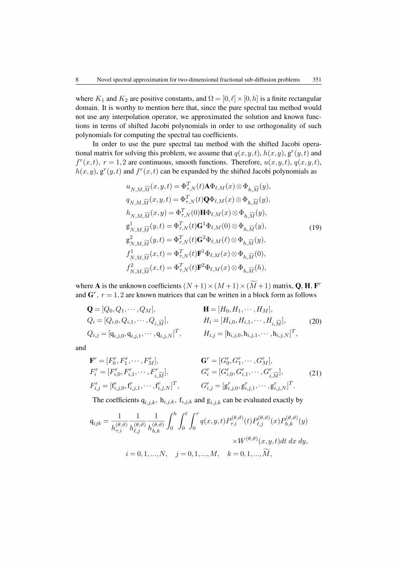
In order to use the pure spectral tau method with the shifted Jacobi opera-tional matrix for solving this problem, we assume that q(x,y, t), h(x,y), gr(y,t) andf r(x,t), r = 1,2 are continuous, smooth functions. Therefore, u(x,y, t), q(x,y, t),h(x,y), gr(y, t) and f r(x,t) can be expanded by the shifted Jacobi polynomials as
uN,M,M
(x,y, t) = ΦTτ,N (t)AΦℓ,M (x)⊗Φ
h,M(y),
qN,M,M
(x,y, t) = ΦTτ,N (t)QΦℓ,M (x)⊗Φ
h,M(y),
hN,M,M
(x,y) = ΦTτ,N (0)HΦℓ,M (x)⊗Φ
h,M(y),
g1N,M,M
(y,t) = ΦTτ,N (t)G1Φℓ,M (0)⊗Φ
h,M(y),
g2N,M,M
(y,t) = ΦTτ,N (t)G2Φℓ,M (ℓ)⊗Φ
h,M(y),
f1N,M,M
(x,t) = ΦTτ,N (t)F1Φℓ,M (x)⊗Φ
h,M(0),
f2N,M,M
(x,t) = ΦTτ,N (t)F2Φℓ,M (x)⊗Φ
h,M(h),
(19)
where A is the unknown coefficients (N+1)× (M +1)× (M +1) matrix, Q, H, Fr
and Gr, r = 1,2 are known matrices that can be written in a block form as follows
Q = [Q0,Q1, · · · ,QM ],
Qi = [Qi,0,Qi,1, · · · ,Qi,M],
Qi,j = [qi,j,0,qi,j,1, · · · ,qi,j,N ]T ,
H = [H0,H1, · · · ,HM ],
Hi = [Hi,0,Hi,1, · · · ,Hi,M],
Hi,j = [hi,j,0,hi,j,1, · · · ,hi,j,N ]T ,
(20)
and
Fr = [F r0 ,F
r1 , · · · ,F r
M ],
F ri = [F r
i,0,Fri,1, · · · ,F r
i,M],
F ri,j = [fri,j,0, f
ri,j,1, · · · , fri,j,N ]T ,
Gr = [Gr0,G
r1, · · · ,Gr
M ],
Gri = [Gr
i,0,Gri,1, · · · ,Gr
i,M],
Gri,j = [gri,j,0,g
ri,j,1, · · · ,gri,j,N ]T .
(21)
The coefficients qi,j,k, hi,j,k, fi,j,k and gi,j,k can be evaluated exactly by
qijk =1
h(θ,ϑ)τ,i
1
h(θ,ϑ)ℓ,j
1
h(θ,ϑ)h,k
∫ h
0
∫ ℓ
0
∫ τ
0q(x,y, t)P
(θ,ϑ)τ,i (t)P
(θ,ϑ)ℓ,j (x)P
(θ,ϑ)h,k (y)
×W (θ,ϑ)(x,y, t)dt dx dy,
i= 0,1, ...,N, j = 0,1, ...,M, k = 0,1, ...,M ,
RJP 60(Nos. 3-4), 344–359 (2015) (c) 2015 - v.1.3a*2015.4.21
352 A.H. Bhrawy et al. 9
hijk =1
h(θ,ϑ)τ,i
1
h(θ,ϑ)ℓ,j
1
h(θ,ϑ)h,k
∫ h
0
∫ ℓ
0
∫ τ
0h(x,y)P
(θ,ϑ)τ,i (t)P
(θ,ϑ)ℓ,j (x)P
(θ,ϑ)h,k (y)
×W (θ,ϑ)(x,y, t)dt dx dy,
i= 0,1, ...,N, j = 0,1, ...,M, k = 0,1, ...,M ,
frijk =1
h(θ,ϑ)τ,i
1
h(θ,ϑ)ℓ,j
1
h(θ,ϑ)h,k
∫ h
0
∫ ℓ
0
∫ τ
0fr(x,t)P (θ,ϑ)
τ,i (t)P(θ,ϑ)ℓ,j (x)P
(θ,ϑ)h,k (y)
×W (θ,ϑ)(x,y, t)dt dx dy,
r = 1,2, i= 0,1, ...,N, j = 0,1, ...,M, k = 0,1, ...,M ,
grijk =1
h(θ,ϑ)τ,i
1
h(θ,ϑ)ℓ,j
1
h(θ,ϑ)h,k
∫ h
0
∫ ℓ
0
∫ τ
0gr(y,t)P (θ,ϑ)
τ,i (t)P(θ,ϑ)ℓ,j (x)P
(θ,ϑ)h,k (y)
×W (θ,ϑ)(x,y, t)dt dx dy,
r = 1,2, i= 0,1, ...,N, j = 0,1, ...,M, k = 0,1, ...,M .
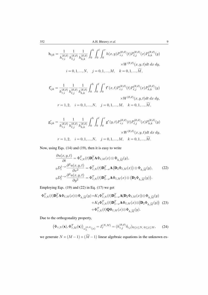
Now, using Eqs. (14) and (19), then it is easy to write
∂u(x,y, t)
∂t=ΦT
τ,N (t)DT1 AΦℓ,M (x)⊗Φ
h,M(y),
0D1−νt
∂2u(x,y, t)
∂x2=ΦT
τ,N (t)DT1−νA
(D2Φℓ,M (x)
)⊗Φ
h,M(y),
0D1−νt
∂2u(x,y, t)
∂y2=ΦT
τ,N (t)DT1−νAΦℓ,M (x)⊗
(D2Φh,M
(y)).
(22)
Employing Eqs. (19) and (22) in Eq. (17) we get
ΦTτ,N (t)DT
1 AΦℓ,M (x)⊗Φh,M
(y)=K1ΦTτ,N (t)DT
1−νA(D2Φℓ,M (x))⊗Φh,M
(y)
+K2ΦTτ,N (t)DT
1−νAΦℓ,M (x)⊗(D2Φh,M
(y))
+ΦTτ,N (t)QΦℓ,M (x)⊗Φ
h,M(y).
(23)
Due to the orthogonality property,(Φτ,N (x),ΦT
τ,M (x))ω(θ,ϑ)L (x)
= I(N,M)τ = (h
(θ,ϑ)τ,j δi,j)0≤i≤N, 0≤j≤M , (24)
we generate N × (M −1)× (M −1) linear algebraic equations in the unknown ex-
RJP 60(Nos. 3-4), 344–359 (2015) (c) 2015 - v.1.3a*2015.4.21
10 Novel spectral approximation for two-dimensional fractional sub-diffusion problems 353
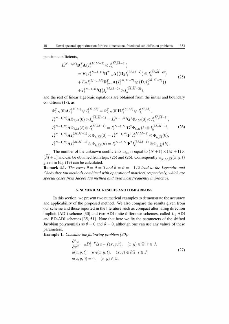
pansion coefficients,
I(N−1,N)τ DT
1 A(I(M,M−2)ℓ ⊗ I
(M,M−2)h
)=K1I
(N−1,M)τ DT
1−νA((
D2I(M,M−2)ℓ
)⊗ I
(M,M−2)h
)+K2I
(N−1,M)τ DT
1−νA(I(M,M−2)ℓ ⊗
(D2I
(M,M−2)h
))+ I(N−1,M)
τ Q(I(M,M−2)ℓ ⊗ I
(M,M−2)h
),
(25)
and the rest of linear algebraic equations are obtained from the initial and boundaryconditions (18), as
ΦTτ,N (0)AI
(M,M)ℓ ⊗ I
(M,M)h =ΦT
τ,N (0)HI(M,M)ℓ ⊗ I
(M,M)h ,
I(N−1,N)τ AΦℓ,M (0)⊗ I
(M,M−1)h = I(N−1,N)
τ G1Φℓ,M (0)⊗ I(M,M−1)h ,
I(N−1,N)τ AΦℓ,M (ℓ)⊗ I
(M,M−1)h = I(N−1,N)
τ G2Φℓ,M (ℓ)⊗ I(M,M−1)h ,
I(N−1,N)τ AI
(M,M−1)ℓ ⊗Φ
h,M(0) = I(N−1,N)
τ F1I(M,M−1)ℓ ⊗Φ
h,M(0),
I(N−1,N)τ AI
(M,M−1)ℓ ⊗Φ
h,M(h) = I(N−1,N)
τ F2I(M,M−1)ℓ ⊗Φ
h,M(h).
(26)
The number of the unknown coefficients aijk is equal to (N +1)× (M +1)×(M+1) and can be obtained from Eqs. (25) and (26). Consequently u
N,M,M(x,y, t)
given in Eq. (19) can be calculated.Remark 4.1. The cases θ = ϑ = 0 and θ = ϑ = −1/2 lead to the Legendre andChebyshev tau methods combined with operational matrices respectively, which arespecial cases from Jacobi tau method and used most frequently in practice.
5. NUMERICAL RESULTS AND COMPARISONS
In this section, we present two numerical examples to demonstrate the accuracyand applicability of the proposed method. We also compare the results given fromour scheme and those reported in the literature such as compact alternating directionimplicit (ADI) scheme [30] and two ADI finite difference schemes, called L1-ADIand BD-ADI schemes [35, 51]. Note that here we fix the parameters of the shiftedJacobian polynomials as θ = 0 and ϑ = 0, although one can use any values of theseparameters.Example 1. Consider the following problem [30]:
∂2u
∂x2= 0D
1−νt ∆u+f(x,y, t), (x,y) ∈ Ω, t ∈ J,
u(x,y, t) = uD(x,y, t), (x,y) ∈ ∂Ω, t ∈ J,
u(x,y,0) = 0, (x,y) ∈ Ω.
(27)
RJP 60(Nos. 3-4), 344–359 (2015) (c) 2015 - v.1.3a*2015.4.21
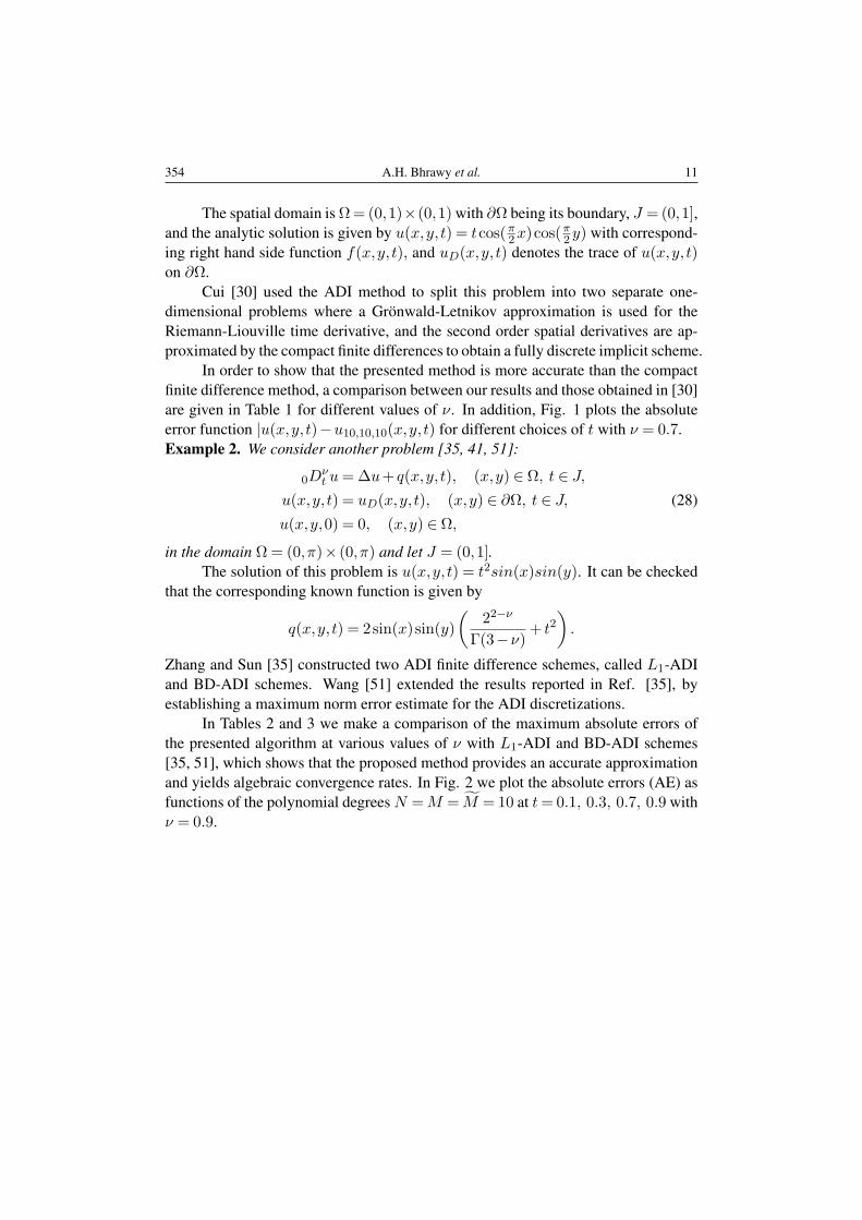
354 A.H. Bhrawy et al. 11
The spatial domain is Ω= (0,1)×(0,1) with ∂Ω being its boundary, J = (0,1],and the analytic solution is given by u(x,y, t) = tcos(π2x)cos(
π2 y) with correspond-
ing right hand side function f(x,y, t), and uD(x,y, t) denotes the trace of u(x,y, t)on ∂Ω.
Cui [30] used the ADI method to split this problem into two separate one-dimensional problems where a Gronwald-Letnikov approximation is used for theRiemann-Liouville time derivative, and the second order spatial derivatives are ap-proximated by the compact finite differences to obtain a fully discrete implicit scheme.
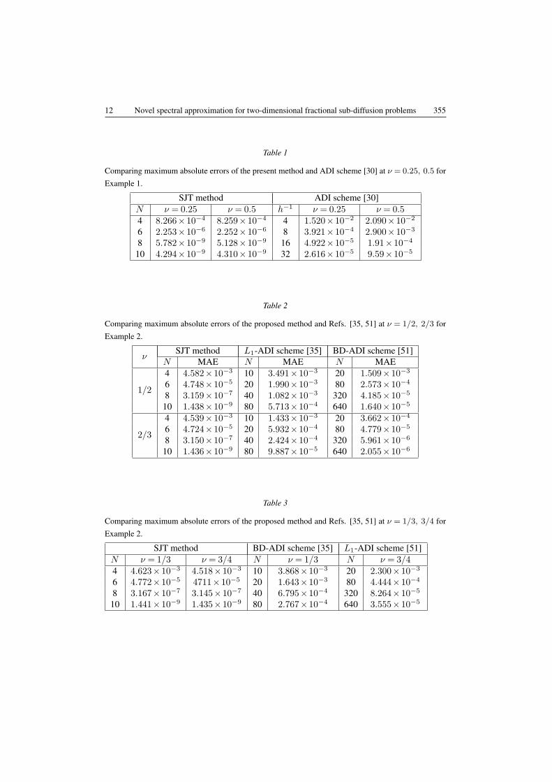
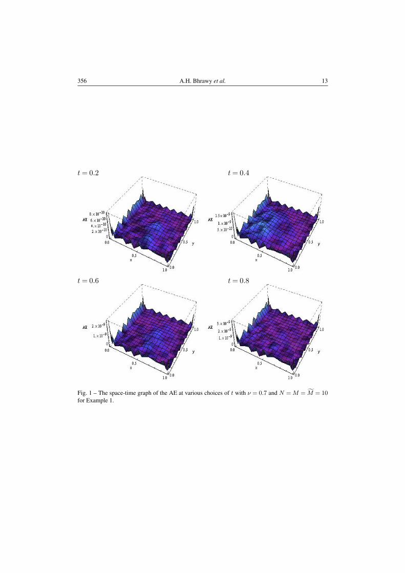
In order to show that the presented method is more accurate than the compactfinite difference method, a comparison between our results and those obtained in [30]are given in Table 1 for different values of ν. In addition, Fig. 1 plots the absoluteerror function |u(x,y, t)−u10,10,10(x,y, t) for different choices of t with ν = 0.7.Example 2. We consider another problem [35, 41, 51]:
0Dνt u=∆u+ q(x,y, t), (x,y) ∈ Ω, t ∈ J,
u(x,y, t) = uD(x,y, t), (x,y) ∈ ∂Ω, t ∈ J,
u(x,y,0) = 0, (x,y) ∈ Ω,
(28)
in the domain Ω= (0,π)× (0,π) and let J = (0,1].The solution of this problem is u(x,y, t) = t2sin(x)sin(y). It can be checked
that the corresponding known function is given by
q(x,y, t) = 2sin(x)sin(y)
(22−ν
Γ(3−ν)+ t2
).
Zhang and Sun [35] constructed two ADI finite difference schemes, called L1-ADIand BD-ADI schemes. Wang [51] extended the results reported in Ref. [35], byestablishing a maximum norm error estimate for the ADI discretizations.
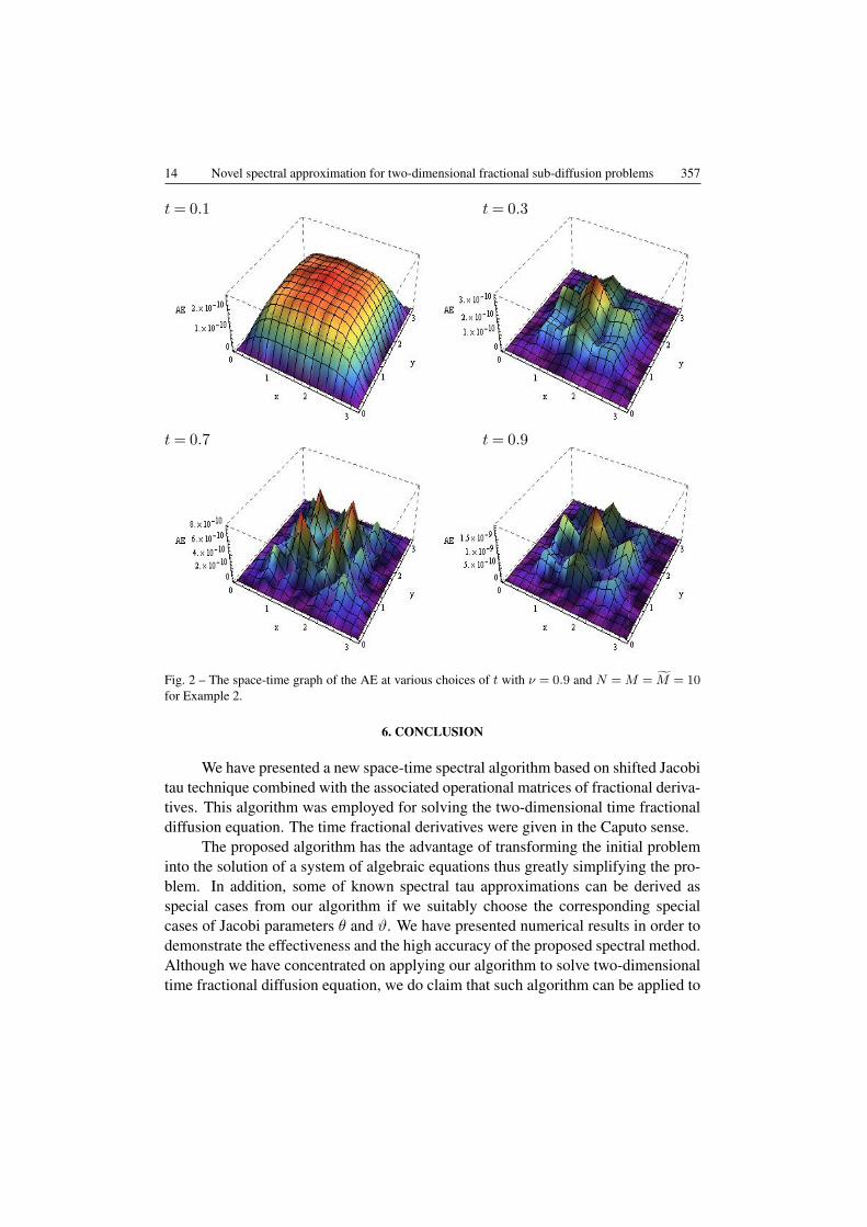
In Tables 2 and 3 we make a comparison of the maximum absolute errors ofthe presented algorithm at various values of ν with L1-ADI and BD-ADI schemes[35, 51], which shows that the proposed method provides an accurate approximationand yields algebraic convergence rates. In Fig. 2 we plot the absolute errors (AE) asfunctions of the polynomial degrees N =M = M = 10 at t= 0.1, 0.3, 0.7, 0.9 withν = 0.9.
RJP 60(Nos. 3-4), 344–359 (2015) (c) 2015 - v.1.3a*2015.4.21
12 Novel spectral approximation for two-dimensional fractional sub-diffusion problems 355
Table 1
Comparing maximum absolute errors of the present method and ADI scheme [30] at ν = 0.25, 0.5 for
Example 1.
SJT method ADI scheme [30]N ν = 0.25 ν = 0.5 h−1 ν = 0.25 ν = 0.54 8.266×10⁻⁴ 8.259×10⁻⁴ 4 1.520×10⁻² 2.090×10⁻²
6 2.253×10⁻⁶ 2.252×10⁻⁶ 8 3.921×10⁻⁴ 2.900×10⁻³
8 5.782×10⁻⁹ 5.128×10⁻⁹ 16 4.922×10⁻⁵ 1.91×10⁻⁴
10 4.294×10⁻⁹ 4.310×10⁻⁹ 32 2.616×10⁻⁵ 9.59×10⁻⁵
Table 2
Comparing maximum absolute errors of the proposed method and Refs. [35, 51] at ν = 1/2, 2/3 for
Example 2.
νSJT method L1-ADI scheme [35] BD-ADI scheme [51]
N MAE N MAE N MAE
1/2
4 4.582×10⁻³ 10 3.491×10⁻³ 20 1.509×10⁻³
6 4.748×10⁻⁵ 20 1.990×10⁻³ 80 2.573×10⁻⁴
8 3.159×10⁻⁷ 40 1.082×10⁻³ 320 4.185×10⁻⁵
10 1.438×10⁻⁹ 80 5.713×10⁻⁴ 640 1.640×10⁻⁵
2/3
4 4.539×10⁻³ 10 1.433×10⁻³ 20 3.662×10⁻⁴
6 4.724×10⁻⁵ 20 5.932×10⁻⁴ 80 4.779×10⁻⁵
8 3.150×10⁻⁷ 40 2.424×10⁻⁴ 320 5.961×10⁻⁶
10 1.436×10⁻⁹ 80 9.887×10⁻⁵ 640 2.055×10⁻⁶
Table 3
Comparing maximum absolute errors of the proposed method and Refs. [35, 51] at ν = 1/3, 3/4 for
Example 2.
SJT method BD-ADI scheme [35] L1-ADI scheme [51]N ν = 1/3 ν = 3/4 N ν = 1/3 N ν = 3/44 4.623×10⁻³ 4.518×10⁻³ 10 3.868×10⁻³ 20 2.300×10⁻³
6 4.772×10⁻⁵ 4711×10−5 20 1.643×10⁻³ 80 4.444×10⁻⁴
8 3.167×10⁻⁷ 3.145×10⁻⁷ 40 6.795×10⁻⁴ 320 8.264×10⁻⁵
10 1.441×10⁻⁹ 1.435×10⁻⁹ 80 2.767×10⁻⁴ 640 3.555×10⁻⁵
RJP 60(Nos. 3-4), 344–359 (2015) (c) 2015 - v.1.3a*2015.4.21
356 A.H. Bhrawy et al. 13
t= 0.2 t= 0.4
t= 0.6 t= 0.8
Fig. 1 – The space-time graph of the AE at various choices of t with ν = 0.7 and N =M = M = 10for Example 1.
RJP 60(Nos. 3-4), 344–359 (2015) (c) 2015 - v.1.3a*2015.4.21
14 Novel spectral approximation for two-dimensional fractional sub-diffusion problems 357
t= 0.1 t= 0.3
t= 0.7 t= 0.9
Fig. 2 – The space-time graph of the AE at various choices of t with ν = 0.9 and N =M = M = 10for Example 2.
6. CONCLUSION
We have presented a new space-time spectral algorithm based on shifted Jacobitau technique combined with the associated operational matrices of fractional deriva-tives. This algorithm was employed for solving the two-dimensional time fractionaldiffusion equation. The time fractional derivatives were given in the Caputo sense.
The proposed algorithm has the advantage of transforming the initial probleminto the solution of a system of algebraic equations thus greatly simplifying the pro-blem. In addition, some of known spectral tau approximations can be derived asspecial cases from our algorithm if we suitably choose the corresponding specialcases of Jacobi parameters θ and ϑ. We have presented numerical results in order todemonstrate the effectiveness and the high accuracy of the proposed spectral method.Although we have concentrated on applying our algorithm to solve two-dimensionaltime fractional diffusion equation, we do claim that such algorithm can be applied to
RJP 60(Nos. 3-4), 344–359 (2015) (c) 2015 - v.1.3a*2015.4.21
358 A.H. Bhrawy et al. 15
solve similar, however more complicated problems in the three-dimensional case.
REFERENCES
1. K.B. Oldham, J. Spanier, The Fractional Calculus (Academic Press, 1974).2. K.S. Miller, B. Ross, An Introduction to the Fractional Calculus and Fractional Differential Equa-
tions (John Wiley, 1993).3. D. Baleanu, K. Diethelm, E. Scalas, J.J. Trujillo, Fractional Calculus Models and Numerical Meth-
ods (World Scientific, Singapore, 2012).4. R.C. Koeller, J. Appl. Mech. 51, 229 (1984).5. J.A. Ochoa-Tapia, F.J. Valdes-Parada, J.A. Alvarez-Ramirez, Physica A 374, 1 (2007).6. M. Axtell, M.E. Bise, Dayton, Proc. IEEE, Dayton, Ohio, USA, pp. 563-566 (1990).7. N. Laskin, Phys. A 287, 482 (2000).8. I.M. Sokolov, J. Klafter, A. Blumen, Phys. Today 55, 48 (2002).9. A. Dokoumetzidis, P. Macheras, J. Pharmacokinet. Pharmacodyn. 36, 165 (2009).
10. R. Schumer, M. Meerschaert, B. Baeumer, J. Geophys. Res.: Earth Surface 114, 2003 (2009).11. F.M. Atici, S. Sengul, J. Math. Anal. Appl. 369, 1 (2010).12. R. Hilfer, Applications of Fractional Calculus in Physics, World Scientific, 2000.13. B. Bonilla, M. Rivero, L. Rodrıguez-Germa, J. Trujillo, Appl. Math. Comput. 187, 79 (2007).14. R. Gorenflo, F. Mainardi, D. Moretti, P. Paradisi, Nonlinear Dyn. 29, 129 (2002).15. O.P. Agrawal, Nonlinear Dyn. 29, 145 (2002).16. R. Metzler, J. Klafter, Phys. Rep. 339, 1 (2000).17. A.H. Bhrawy, D. Baleanu, Rep. Math. Phys. 72, 219 (2013).18. A.H. Bhrawy, Abstr. Appl. Anal. 2013, Article ID 954983 (2013).19. S. Chen, F. Liu, X. Jiang, I. Turner, V. Anh, Appl. Math. Comput. DOI: 10.1016/j.amc.2014.08.031
(2014).20. X.-J. Yang, D. Baleanu, Y. Khan, S.T. Mohyud-Din, Rom. J. Phys. 59, 36 (2014).21. A.H. Bhrawy, Abstr. Appl. Anal. 2014, 10 (2014).22. E.H. Doha, A.H. Bhrawy, S.S. Ezz-Eldien, Centr. Eur. J. Phys. 11, 1494 (2013).23. Z. Wang, S. Vong, J. Comput. Phys. 277, DOI: 10.1016/j.jcp.2014.08.012 (2014).24. S. B. Yuste, J. Comput. Phys. 216, 264 (2006).25. C. M. Chen, F. Liu, I. Turner, V. Anh, J. Comput. Phys. 227, 886 (2007).26. T.A.M. Langlands, B.I. Henry, J. Comput. Phys. 205, 719 (2005).27. P. Zhuang, F. Liu, V. Anh, I. Turner, SIAM J. Numer. Anal. 46, 1079 (2008).28. Z.Z. Sun, X.N. Wu, Appl. Numer. Math. 56, 193 (2006).29. M. Cui, J. Comput. Phys. 228, 7792 (2009).30. M. Cui, J. Comput. Phys.231, 2621 (2012).31. G.H. Gao, Z.Z. Sun, J. Comput. Phys. 230, 586 (2011).32. P. Zhuang, F. Liu, V. Anh, I. Turner, SIAM J. Numer. Anal. 47, 1760 (2009)33. H.R. Ghazizadeh, M. Maerefat, A. Azimi, J. Comput. Phys. 229, 7042 (2010).34. P. Zhuang, F. Liu, V. Anh, I. Turner, IMA J. Appl. Math. 74, 645 (2009).35. Y. Zhang, Z. Sun, J. Comput. Phys. 230, 8713 (2011).36. X. Lin, C. Xu, J. Comput. Phys. 225, 1533 (2007).37. X. Li, C. Xu, SIAM J. Numer. Anal. 47, 2108 (2009).38. H. Brunner, L. Ling, M. Yamamoto, J. Comput. Phys. 229, 6613 (2010).
RJP 60(Nos. 3-4), 344–359 (2015) (c) 2015 - v.1.3a*2015.4.21
16 Novel spectral approximation for two-dimensional fractional sub-diffusion problems 359
39. A.H. Bhrawy, E.H. Doha, D. Baleanu, S.S. Ezz-Eldien, J. Comput. Phys.,DOI:10.1016/j.jcp.2014.03.039 (2014).
40. E.H. Doha, A.H. Bhrawy, S.S. Ezz-Eldien, J. Comput. Nonlinear Dyn., DOI:10.1115/1.4027944(2014).
41. X. Yang, H. Zhang, D. Xu, J. Comput. Phys. 256, 824 (2014).42. E.H. Doha, A.H. Bhrawy, D. Baleanu, M.A. Abdelkawy, Rom. J. Phys. 59, 247 (2014).43. E.H. Doha, A.H. Bhrawy, D. Baleanu, M.A. Abdelkawy, Rom. J. Phys. 59, 408 (2014).44. A. Jafarian et al., Rom. Rep. Phys. 66, 296 (2014).45. A. Jafarian et al., Rom. Rep. Phys. 66, 603 (2014).46. E.H. Doha, A.H. Bhrawy, D. Baleanu, R.M. Hafez, Appl. Numer. Math. 77, 43 (2014).47. E.H. Doha, D. Baleanu, A.H. Bhrawy, R.M. Hafez, Proc. Romanian Acad. A 15, 130 (2014).48. A.H. Bhrawy, E.A. Ahmed, D. Baleanu, Proc. Romanian Acad. A 15, 322 (2014).49. I. Podlubny, A. Chechkin, T. Skovranek, Y. Chen, B.M. Vinagre Jara, J. Comput. Phys. 228, 31
(2009).50. E.H. Doha, A.H. Bhrawy, S.S. Ezz-Eldien, Appl. Math. Model. 36, 4931 (2012).51. Y.M. Wang, Adv. Math. Phys. 6, 130258 (2013).
RJP 60(Nos. 3-4), 344–359 (2015) (c) 2015 - v.1.3a*2015.4.21