Solar Cells, 25 ( 1 9 8 8 ) 127 - 142 127

A NOVEL METHOD FOR DETERMINING THE OPTIMUM SIZE OF STAND-ALONE PHOTOVOLTAIC SYSTEMS

C. SORAS and V. MAKIOS

Laboratory of Electromagnetics, Department of Electrical Engineering, University of Patras, Patras (Greece)

(Received July 8, 1988; accepted August 8, 1988)

Summary

A method is presented to select the optimum tilt angle, photovoltaic array area and battery storage capacity of stand-alone photovoltaic systems. This method uses monthly average meteorological data and easily acquirable system parameters in order to determine possible photovoltaic system sizes, capable of supplying any given monthly average hourly load profile. The optimum system selected is that with the minimum life-cycle cost while ensuring a desired reliability level. In the life-cycle cost computations a battery-life model has been used to determine the number of battery bank replacements. The reliability criterion used is the loss-of-energy probability. The method can be implemented on a personal computer and is applied to an illustrative example, where the optimum system size proposed by this methodology is compared with that of a newly installed system on a Greek island.

1. Introduction

The existence of analytical methods for selecting the optimum size of stand-alone photovoltaic (SAPV) systems, is the basic requirement for their proliferation. Depending on the approach used to estimate the system performance, which is the prerequisite in any system sizing process, two solutions related to the system sizing problem can be identified, namely detailed simulations and simplified design methods.

The models which perform detailed photovoltaic system simulation, e.g. ref. 1, calculate deterministically the energy flow into the system for each hour during the whole period of the analysis, using historical data of solar radiation and ambient temperature. Although these models provide an adequate solution to the system sizing problem, they feature some significant disadvantages, i.e. large computing time, not easily acquirable system parameter values and the need of long-term hourly meteorological data, which are not available for most locations worldwide.

0 3 7 9 - 6 7 8 7 / 8 8 / $ 3 . 5 0 © Elsevier Sequo i a /P r in t ed in The Ne the r l ands

128

The difficulties of the above models have led to the development of simplified methods that, without giving the variety of information of the detailed models, are able to select the opt imum system size, though with differing degree of success (Section 2). In this paper a new methodology is described (Section 4) which overcomes the limitations of the existing methods. The proposed method is used in an illustrative example in Section 5 where the system size proposed is compared with a newly installed system on a Greek island.

2. Review of the existing system sizing methodologies

Most of the simplified methods which have been developed so far for stand-alone systems [ 2 - 6 ] are based on the comparison between the monthly average daily photovoltaic system output for an array of a given size and tilt angle and the average daily load. The year round energy deficits dictate the long-term storage capacity which added to the short-term storage determines the effective capacity of the battery and consequently its rated value. By varying the tilt angle and size of the array and computing the cor- responding storage capacity, a number of candidate photovoltaic system sizes are created, among which the most economical is selected as the optimum. The simplicity and applicability to a wide range of configurations are the main advantages of these methods. However, they ignore the effect of supply reliability on system size and hourly variation of both solar radia- t ion and load demand on the calculation of system performance.

An extremely simple method for the selection of system size based on a predetermined probability of system outage due to weather variations, has been proposed by Evans e t al. [7]. This method, however, proposes only one system size which naturally is not the most economical.

Barra e t al. [8] have proposed another analytical method for the deter- mination of the optimal size of SAPV systems, which is based on a predeter- mined uncovered energy load fraction. Uncovered load fraction, however, is not a measure of reliability but only an indication, stating that smaller uncovered fractions result in higher reliability. Further drawbacks of this method are: the assumption that all the energy produced by the photo- voltaic array passes through the battery, and the use of initial investment as the economic criterion, which does not take into account the effect of the number of battery replacements.

A method which takes into account the effect of reliability on system size has also been developed [9, 10]. The method is limited to one value of loss-of-energy probability (LOEP) and two array tilts. Furthermore this method assumes that all the energy from the photovoltaic array passes through the battery, it is based on daily (not hourly) values of solar radiation and load, and does not consider the effect of system performance on battery lifetime.

129

3. Definition of the problem

SAPV systems exhibit the following contradiction: although they are the first systems put into use and have the highest arithmetic percentage of applications of all photovoltaic systems, they are the most difficult to deter- mine their opt imum size, due to the use of batteries as the sole back-up source which influences immensely the reliability of the whole photovoltaic system. The opt imum size, therefore, cannot be determined independently of the load supply reliability which it ensures. The sizing problem could be finally summarized as follows.

Which is the combination of the size A of the photovoltaic array, its tilt angle s and the rated bat tery capacity B, that satisfies a predetermined reliability goal and is the most economical?

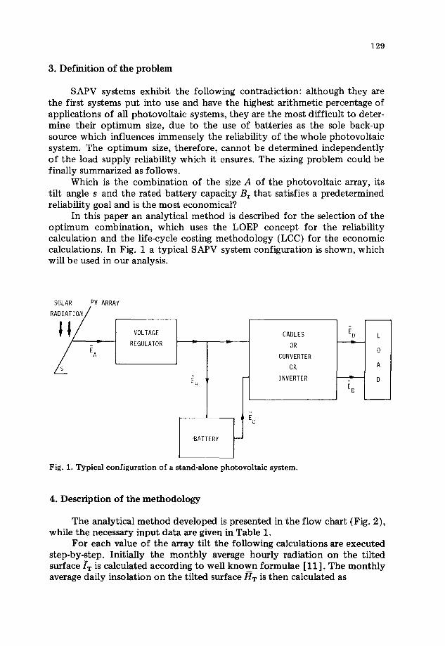
In this paper an analytical method is described for the selection of the opt imum combination, which uses the LOEP concept for the reliability calculation and the life-cycle costing methodology (LCC) for the economic calculations. In Fig. 1 a typical SAPV system configuration is shown, which will be used in our analysis.

SOLAR PV ARRAY RADIATION/

/ /

VOLTAGE REGULATOR

EB

"BATTERY i Ec

Fig. 1. Typicalconfiguration of a stand-alone photovoltaic system.

CABLES OR

CONVERTER OR

INVERTER

ED

4. Description of the methodology

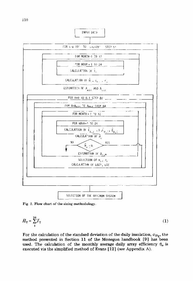
The analytical method developed is presented in the flow chart (Fig. 2), while the necessary input data are given in Table 1.

For each value of the array tilt the following calculations are executed step-by-step. Initially the monthly average hourly radiation on the tilted surface i T is calculated according to well known formulae [11 ]. The monthly average daily insolation on the tilted surface/TT is then calculated as

130

FOR s=q~-lO °

INPUT DATA

I TO s=(p+20' STEP 5 °

FOR MONTH=I TO 12

FOR HOUR= I TO 24

CALCULATION OF l ' r

CALCULATION OF H'r' °ll'I' ' n

ESTIMATION OF A . AND A m l n m & x

FOR U=O TO 0.1 STEP AU

FOR A=Amin TO Amax STEP ~A

FOR MONTH= I TO 12

FOR HOUR=I TO 24

CALCULATION OF EA, i ,$ ,E~3,i , ED, I

CALCULATION OF c~

N ~ YES

ESTIMATION OF Be, m I SELECTION OF Be, B r

CALCULATION OF LOEP, LEC

I SELECTION OF THE OPTIMUM SYSTEM

Fig. 2. Flow chart of the sizing methodology.

24 /qW =~/T (1)

1

For the calculation of the standard deviation of the daily insolation, O~HT , the method presented in Section 11 of the Monegon handbook [9] has been used. The calculation of the monthly average daffy array efficiency ~/e is executed via the simplified method of Evans [12] (see Appendix A).

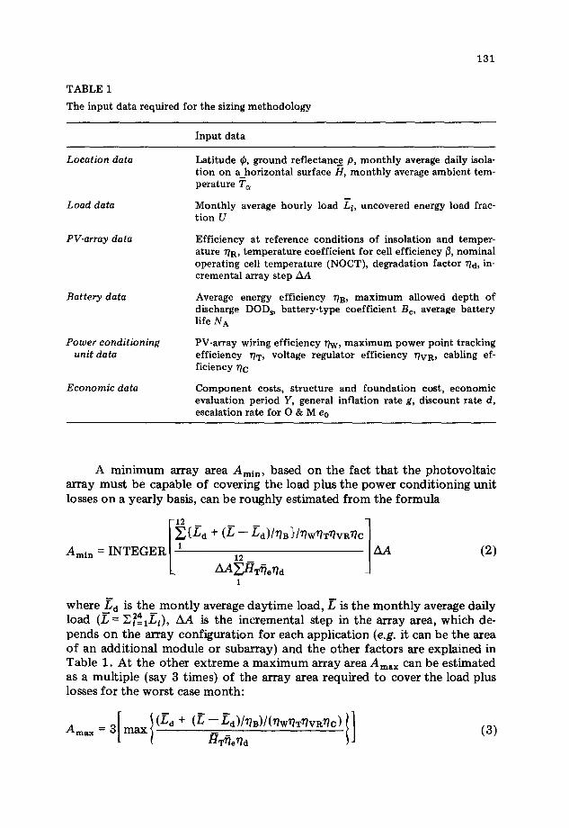
TABLE 1

The input data required for the sizing methodology

131

Input data

Location data

Load data

PV-array data

Battery data

Power conditioning unit data

Economic data

Latitude ¢, ground reflectance p, monthly average daily isola- tion on a horizontal surface H, monthly average ambient tem- perature Ta

Monthly average hourly load Li, uncovered energy load frac- tion U

Efficiency at reference conditions of insolation and temper- ature ~TR, temperature coefficient for cell efficiency ~, nominal operating cell temperature (NOCT), degradation factor 77d, in- cremental array step AA

Average energy efficiency 77B, maximum allowed depth of discharge DODs, battery-type coefficient Bc, average battery life N A

PV-array wiring efficiency ~w, maximum power point tracking efficiency ~TT, voltage regulator efficiency WVR, cabling ef- ficiency r/c

Component costs, structure and foundation cost, economic evaluation period Y, general inflation rate g, discount rate d, escalation rate for O & M e 0

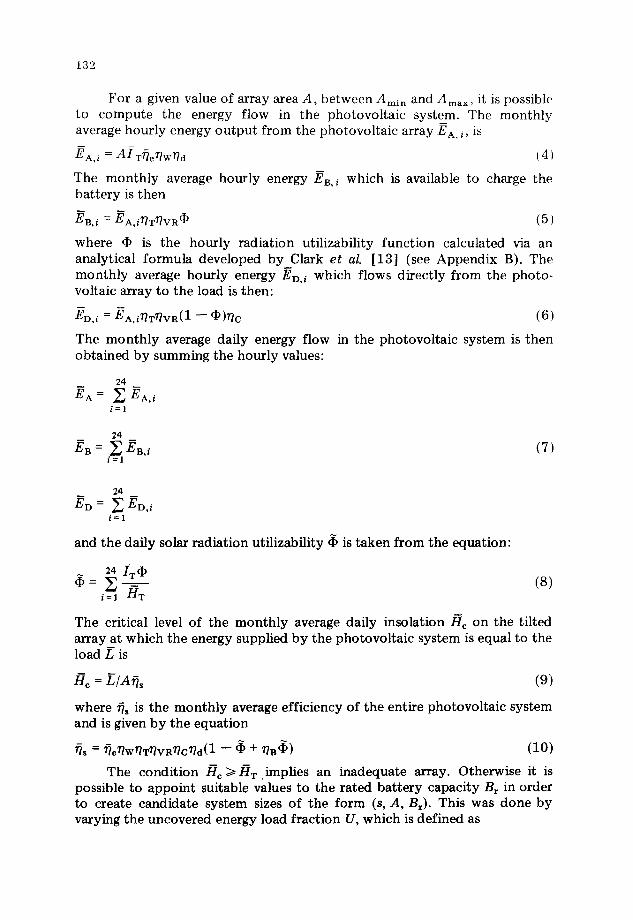
A m i n i m u m ar ray area Amin, based on the fac t t h a t the p h o t o v o l t a i c a r ray m u s t be capab le o f cover ing the load plus t he p o w e r cond i t ion ing uni t losses on a yea r ly basis, can be rough l y e s t ima ted f r o m the f o r m u l a

Ami n = I N T E G E R [ -I - ~ [ A A

~ ' ~ T ~ e n d J 1

(2)

where Ld is the montly average daytime load, L is the monthly average daily load (L = Z24 ~- ~=l~J, AA is the incremental step in the array area, which de- pends on the array configuration for each application (e.g. it can be the area of an additional module or subarray) and the other factors are explained in Table 1. At the other extreme a maximum array area Am~x can be estimated as a multiple (say 3 times) of the array area required to cover the load plus losses for the worst case month:

Amax = 3[ max{ (f'a +(L--~d)/~B)/(~W~T~V~C)}] I'IT~eT~d

(3)

132

For a given value of array area A, between Ami n and Amax, it is possible to compute the energy flow in the photovoltaic system. The monthly average hourly energy output from the photovoltaic array ]~A, i, is

EA,i = A/w~eT~W7~d ( 4 )

The monthly average hourly energy /Ts, i which is available to charge the battery is then

EB, i = /~A, iT~T?TVR fl) (5)

where (P is the hourly radiation utilizability function calculated via an analytical formula developed by Clark e t al. [13] (see Appendix B). The monthly average hourly energy ED, i which flows directly from the photo- voltaic array to the load is then:

/~D,i = EA, iT~T~/VR(I -- CI~)~/C (6)

The monthly average daffy energy flow in the photovoltaic system is then obtained by summing the hourly values:

24 EA = E gA, i

i = l

24 EB = ~ E~,i (7)

i=l

24 ED = 2: ~D,i

i = l

and the daffy solar radiation utffizability c~ is taken from the equation:

24 IT~ = E tTT (8) i = l

The critical level of the monthly average daffy insolation /~c on the tilted array at which the energy supplied by the photovoltaic system is equal to the load/~ is

H c = Y,/A~?s (9)

where ~, is the monthly average efficiency of the entire photovoltaic system and is given by the equation

~s = ~Ter/W~T?/VR~TCr/d( 1 -- ~ + ?/B c~) (I0)

The condition /~c ~>/~T implies an inadequate array. Otherwise it is possible to appoint suitable values to the rated battery capacity B~ in order to create candidate system sizes of the form (s, A, Br). This was done by varying the uncovered energy load fraction U, which is defined as

133

U = I -- f (11 )

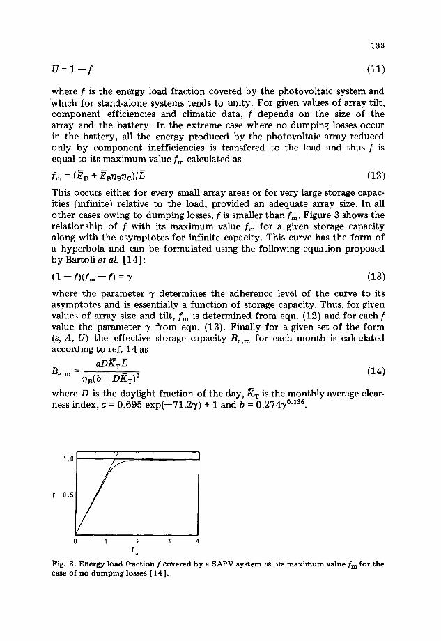
where f is the energy load fraction covered by the photovoltaic system and which for stand-alone systems tends to unity. For given values of array tilt, component efficiencies and climatic data, f depends on the size of the array and the battery. In the extreme case where no dumping losses occur in the battery, all the energy produced by the photovoltaic array reduced only by component inefficiencies is transfered to the load and thus f is equal to its maximum value fm calculated as

fm ---- (ED "{- J~B?~B~C)/j~ (12)

This occurs either for every small array areas or for very large storage capac- ities (infinite) relative to the load, provided an adequate array size. In all other cases owing to dumping losses, f is smaller than fro. Figure 3 shows the relationship of f with its maximum value fm for a given storage capacity along with the asymptotes for infinite capacity. This curve has the form of a hyperbola and can be formulated using the following equation proposed by Bartoli e t al. [14] :

(I -- f)(fm -- f) = ~/ (13)

where the parameter ~/ determines the adherence level of the curve to its asymptotes and is essentially a function of storage capacity. Thus, for given values of array size and tilt, fm is determined from eqn. (12) and for each f value the parameter ~/ from eqn. (13). Finally for a given set of the form (s, A, U) the effective storage capacity Be,~ for each month is calculated according to ref. 14 as

aDKTL Be,m ~B(b + D/~T) 2 (14)

where D is the daylight fraction of the day,/~T is the monthly average clear- ness index, a = 0.695 exp(--71.2"y) + 1 and b = 0.274T o'la6.

1.0

f 0.5

0 I 2 3 fm

Fig. 3. Energy load fraction f covered by a SAPV system vs. its maximum value fm for the case of no dumping losses [14].

134

The month with the maximum storage requirements dictates the ef- fective bat tery capacity which corresponds to the given values of s, U and A :

Be = max(Be.m) (15)

The rated bat tery capacity is then:

B~ = Be /DODs (16)

where DODs is the maximum allowable depth of discharge of the bat tery during its seasonal operation.

For each candidate photovoltaic system size of the form (s, A, B~) the supply reliability it ensures is calculated in terms of the yearly LOEP which b y definition [15] is the sum of the monthly values LOEPM:

12 LOEP = ~ LOEPM (17)

M=I

The method used for the LOEPM calculation was that°described in ref. 9. For each candidate size besides LOEP, its levelized energy cost, LEC, is also computed using the methodology of Appendix C, where a model of bat tery life is used for the estimation of the number of bat tery replacements through the system lifetime.

5. A sizing example

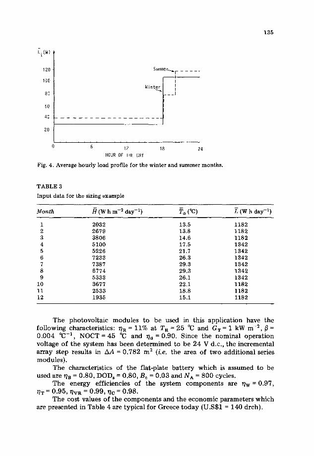
Let us consider the case of a remote house for which we intend to cover the basic energy needs in terms of lighting, radio, television and re- frigeration. The load characteristics assumed are presented in Table 2 and the resulting load profile in Fig. 4, The house is located on a Greek island, Antikythira, with ¢ = 36 °, p = 0.2. The monthly average values of insolation /7 on a horizontal surface, ambient temperature T~ and load/~ are presented in Table 3.

T A B L E 2

R e m o t e h o u s e load characteristics

Appliance Nominal power Hours in operation

(W) Winter Summer

2 f l u o r e s c e n t l a m p s 2 × 20 18 .00 - 24 .00 20 .00 - 24 .00

R e f r i g e r a t o r 30 (Win te r ) 0 .00 - 24 .00 0 .00 - 24 .00 (115 l) 40 ( S u m m e r )

T V (17 in) C o l o u r 37 18 .00 - 24 .00 18 .00 - 24 .00

Ci(w)

120

100

80

60

40

20

Summer--~ F . . . . . !

I Wint 1

6 12 18 24

HOUR OF THE DAY

Fig. 4. Average hourly load profile for the winter and summer months.

135

TABLE 3

Input data for the sizing example

M o n t h /~ (W h m -2 day -1) Ta (°C) L (W h day -1)

1 2032 13.5 1182 2 2679 13.8 1182 3 3806 14.6 1182 4 5100 17.5 1342 5 5226 21.7 1342 6 7233 26.3 1342 7 7387 29.3 1342 8 6774 29.3 1342 9 5333 26.1 1342

10 3677 22.1 1182 11 2533 18.8 1182 12 1935 15.1 1182

T h e p h o t o v o l t a i c m o d u l e s to be used in this app l i ca t ion have the fo l lowing character is t ics : ~?R = 11% at TR = 25 °C and GT = 1 kW m -2, ~ = 0 .004 °C -1 , N O C T = 45 °C and ~d = 0.90. Since the n o m i n a l o p e r a t i o n vol tage o f t he s y s t e m has b e e n d e t e r m i n e d to be 24 V d.c. , the i nc remen ta l a r r ay s tep resul ts in AA = 0 .782 m 2 (i.e. the area o f two add i t iona l series modu les ) .

T h e charac ter i s t ics o f t he f la t -p la te b a t t e r y which is a s sumed to be used are ~?B = 0 .80, D O D s = 0 .80 , Bc = 0 .03 and NA = 800 cycles.

T h e ene rgy eff ic iencies o f the s y s t e m c o m p o n e n t s are ~?w = 0.97, 7~T = 0.95, ~VR = 0 .99 , ~C = 0 .98.

T h e cos t values o f t he c o m p o n e n t s and the e c o n o m i c p a r a m e t e r s wh ich are presented in Table 4 are typical for Greece today (U.S$1 = 140 drch).

136

T A B L E 4

Cost and e c o n o m i c assumpt ions

A r r a y cos t Battery cost Structure and f o u n d a t i o n cos t Vo l tage regulator cost Electrical sys tem cost E c o n o m i c evaluat ion period General inf lat ion rate Escalat ion rate for O & M Discount rate

- l Cc~ = 15 $ Wp C b = 2 0 0 $ k W 1 h 1

1 C s = 0 . 9 $ Wp C r = 8 5 0 $

C e = 7 0 0 $

Y = 20 yrs g = 0 ,15 e 0 = 0 .12 d = 0 .17

15 14

13 12 11 10

mo ° 9 .W 8

~< 7

6 L , J k ' - -

5

.~ 4

'- 3 2 1

0

s=45 °

01[~ I i ~ LOEP ...................... ..............................................................................................

O- 3 .......... . ......................................................................................................

10

~I, I ~.:'2' .... ~ .......................... " . , . . . . . . " . . . . . . . . . . . . . . . . . . . . . . . . . . . . . . . . . . . . . . . . . . . . . . . . . . . . . . . . . . . . . . . . . . . . . .

26,10-2 .. . .

0,1

7-/4 860 946 1032 ' 1204 1376 1548 1720 1892 ' 2064

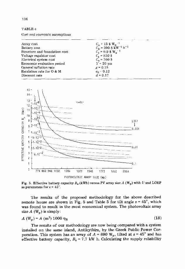
PHOTOVOLTAIC ARRAY SIZE (Wp) Fig. 5. Effect ive battery capac i ty B e (kWh) ve rsus PV a r ray size A (Wp) w i t h U and L O E P

as parameters for s = 45 °.

The results of the proposed m e t h o d o l o g y for the above described remote house are s h o w n in Fig. 5 and Table 5 for tilt angle s = 45 °, which was f o u n d to result in the most e conomica l system. The photovo l ta i c array size A (Wp) is s imply:

A (Wp) = A (m 2) 1 0 0 0 17 R (18)

The results o f our m e t h o d o l o g y are n o w being compared wi th a system installed on the same island, Ant ikythira , by the Greek Public Power Cor- porat ion. This system has an array o f A = 690 Wp, t i l ted at s = 45 ° and has effect ive battery capacity , Be = 7.7 kW h. Calculating the supply reliability

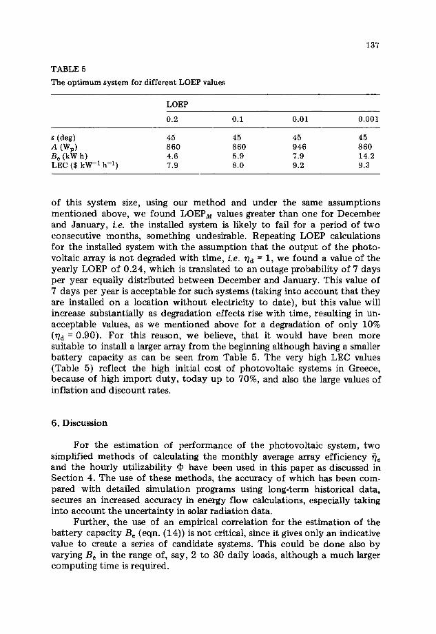
TABLE 5

The optimum system for different LOEP values

137

LOEP

0.2 0.1 0.01 0.001

s (deg) 45 45 45 45 A (Wp) 860 860 946 860 B e (kW h) 4.6 5.9 7.9 14.2 LEC ($ kW -1 h -1) 7.9 8.0 9.2 9.3

of this system size, using our method and under the same assumptions mentioned above, we found LOEPM values greater than one for December and January, i.e. the installed system is likely to fail for a period of two consecutive months, something undesirable. Repeating LOEP calculations for the installed system with the assumption that the output of the photo- voltaic array is not degraded with time, i.e. ~d = 1, we found a value of the yearly LOEP of 0.24, which is translated to an outage probability of 7 days per year equally distributed between December and January. This value of 7 days per year is acceptable for such systems (taking into account that they are installed on a location without electricity to date), but this value will increase substantially as degradation effects rise with time, resulting in un- acceptable values, as we mentioned above for a degradation of only 10% 0?d = 0.90). For this reason, we believe, that it would have been more suitable to install a larger array from the beginning although having a smaller bat tery capacity as can be seen from Table 5. The very high LEC values (Table 5) reflect the high initial cost of photovoltaic systems in Greece, because of high import duty, today up to 70%, and also the large values of inflation and discount rates.

6. Discussion

For the estimation of performance of the photovoltaic system, two simplified methods of calculating the monthly average array efficiency Re and the hourly utilizability dp have been used in this paper as discussed in Section 4. The use of these methods, the accuracy of which has been com- pared with detailed simulation programs using long-term historical data, secures an increased accuracy in energy flow calculations, especially taking into account the uncertainty in solar radiation data.

Further, the use of an empirical correlation for the estimation of the bat tery capacity Be (eqn. {14)) is not critical, since it gives only an indicative value to create a series of candidate systems. This could be done also by varying Be in the range of, say, 2 to 30 daffy loads, although a much larger computing time is required.

138

In conclusion, the novel m e t h o d deve loped in this paper to select the o p t i m u m size of SAPV systems has the advantages of all simplified methods , i.e. use of m o n t h l y average meteoro logica l data, easily acquirable sys tem pa ramete r values and small calculat ion t ime in a PC system. More- over, it possesses the fo l lowing character is t ic advantages which in previous m e t h o d s are no t usually t aken into account .

(a) It uses the LOEP cri ter ion, a widely used rel iabil i ty concep t in power systems, having the advantage of taking into acco u n t the cost vs. rel iabi l i ty t rade-of f in system sizing. LOEP also provides a c o m m o n base for compar i son wi th o the r systems e.g. a diesel generator .

(b) I t is appl icable fo r any m o n t h l y average hour ly load profi le. (c) By using the ut i l izabi l i ty concep t , it raises the accuracy of calcula-

t i on o f sys tem pe r fo rmance , because it does no t use the wrong assumpt ion tha t all energy passes t h rough the ba t t e ry .

(d) It uses a mode l fo r the ba t t e ry l i fet ime based on its average daily de p th o f discharge and the specific characteris t ics of the t y p e o f ba t te ry .

(e) It uses as the economic cr i ter ion the life cycle cost m e t h o d o l o g y , which is mos t appropr ia te fo r solar energy systems.

A c k n o w l e d g m e n t

The au thor s would like to t hank Dr. J. Milias-Argitis fo r m a n y f ru i t fu l discussions and his valuable assistance for the graphical p resen ta t ion o f the results.

References

1 E. Hoover, SOLCEL-II: An improved photovoltaic system analysis program, Sandia National Laboratories Rep. SAND 79-1785, 1980 (Sandia National Laboratories, Albuquerque, NM).

2 Solar Power Corporation, Solar Electric Generator Systems; Principles of operation and design concepts, 1979.

3 C. Soras and V. Makios, Feasible stand-alone photovoltaic systems in Greece, Proc. 5th Eur. Photovoltaic Solar Energy Conf, Athens, Reidel, Dordrecht, 1983, p. 485.

4 M. Buresch, Photovoltaic Energy Systems; Design and Installation, McGraw-Hill, New York, 1983.

5 PRC Energy Analysis Company, Solar photovoltaic applications seminar: design, installation and operation of small stand-alone photovoltaic power systems, U.S. DOE/CS/32522-T1, 1980 (Department of Energy, Washington, DC).

6 Monegon Ltd., Designing small photovoltaic power systems, No. M l l l , 1981. 7 D. L. Evans and F. T. C. Barrels, Battery sizing criteria for stand-alone photovoltaic

power systems, AS/ISES, Philadelphia, PA, 1981. 8 L. Barra, S, Catalanotti, F. Fontana and F. Lavorante, An analytical method to deter-

mine the optimal size of a photovoltaic plant, Sol. Energy, 33 (1984) 509. 9 H. L. Macomber, J. B. Ruzek, F. A. Costello and staff of Bird Engineering, Photo-

voltaic Stand-Alone Systems: Preliminary Engineering Design Handbook, NASA CR-165352, (NASA Lewis Research Center), 1981.

10 P. Groumpos and G. Papageorgiou, An optimal sizing method for stand-alone photo- voltaic power systems, Sol. Energy, 38 (1987) 341.

139

11 J. A. Duffie and W. A. Beckman, Solar Engineering of Thermal Processes, Wiley- Interscience, New York, 1980.

12 D. L. Evans, Simplified method for predicting photovoltaic array output, Sol. Energy, 27 (1981) 555.

13 D. R. Clark, S. A. Klein and W. A. Beckman, Algorithm for evaluating the hourly radiation utilizability function, J. Sol. Energy Eng., 105 (1983) 281.

14 B. Bartoli, U. Coscia, V. Cuomo, F. Fontana and V. Silvestrini, Statistical approach to long-term performances of photovoltaic systems, Rev. Phys. Appl., 18 (1983) 281.

15 R. Billinton, Power System Reliability Evaluation, Gordon and Breach, New York, 1970.

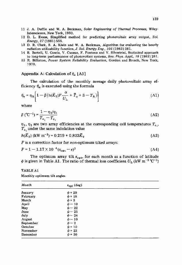
Appendix A: Calculation of ~ [A1]

The calculation of the monthly average daily photovoltaic array ef- ficiency ~e is executed using the formula

a - - TR)] = - - + T ~ + 3 ~, ~Ta 1 /3(h(/~T)F UL (A1)

where

1 - - ~72/7~1 (°C -1) - (A2) Tc~ - - Tel

~71,772 are t w o array eff ic iencies at the corresponding cell temperatures T c,, Tc: under the same indo la t ion value

h(/~T) (kW m -z) = 0 . 2 1 9 + 0.832/~T (A3)

F is a correct ion factor for n o n - o p t i m u m ti l ted arrays:

F = 1 - - 1 .17 × 10 -4 (Sopt - - s ) 2 (A4)

The o p t i m u m array tilt Sopt, for each m o n t h as a f u n c t i o n o f lat i tude ¢ is given in Table A1 . The ratio o f thermal loss coef f ic ient U L (kW m -2 °C-I)

TABLE A1

Monthly optimum tilt angles

Month Sop t (deg)

January ~b + 29 February ~b + 18 March ~b + 3 April ~b- 10 May ~ -- 22 June ~b -- 25 July ~b- 24 August ~b- 10 September ¢ - 2 October ¢ + 10 November ~b + 23 December ¢ + 30

140

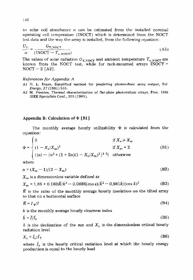
to solar cell absorbance a can be es t imated f rom the installed nominal opera t ing cell t empe ra tu r e ( INOCT) which is de t e rmined f rom the NOCT test da ta and the way the array is installed, f r o m the fol lowing equat ion :

UL GT,NOCT - ( A 5 )

a ( INOCT -- T~,NOCT)

The values of solar rad ia t ion GT, NOGT and ambien t t em p e ra tu r e Tc~,NOC w are k n o w n f r om the NOCT test, while for r ack -moun ted arrays INOCT = N O C T - - 2 [A2] .

R e f e r e n c e s f o r A p p e n d i x A A1 D. L. Evans, Simplified method for predicting photovoltaic array output, Sol.

Energy, 27 (1981) 555. A2 M. Fuentes, Thermal characterization of flat-plate photovoltaic arrays, Proc. 18th

IEEE Specialists Conf., 203 (1985).

A ppe nd ix B: Calcula t ion o f ~ [B1]

The m o n t h l y average hour ly ut i l izabi l i ty equa t ion :

i ° or= (1--XdXm) 2

( I ] ~ ] - - {~2 + (1 + 2a) (1 - - X e / X m ) 2 ) I / 2 [ %

where

o~ = (Xm - - 1)/(2 -- Xm)

X m is a dimensionless variable def ined as

4p is calculated f ro m the

if X c ~ X m

i fXm = 2

o therwise

(B1)

(B2)

X m = 1.85 + 0 .169/~/k 2 -- 0 .0696(cos S ) / k 2 - - 0 .981k / ( cos 5) 2 (B3)

/~ is the rat io o f the m o n t h l y average hour ly insolat ion on the t i l ted array to tha t on a hor izon ta l surface

R = I w / I (B4)

is t he m o n t h l y average hour ly clearness index

k = I / I o (B5)

5 is the dec l ina t ion of the sun and X c is t he dimensionless crit ical hou r ly radia t ion level

Xe = f c / i T (B6)

where i c is the hou r ly critical radia t ion level at which the hour ly energy p r o d u c t i o n is equal to the hour ly load

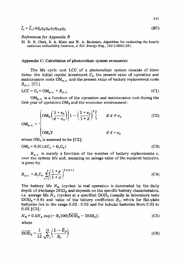
141

References for Appendix B Bl D. R. Clark, S. A. Klein and W. A. Beckman, Algorithm for evaluating the hourly

radiation utilizability function, J. Sol. Energy Eng., 105 (1983) 281.

Appendix C: Calculation of photovoltaic system economics

The life cycle cost LCC of a photovoltaic system consists of three items: the initial capital investment Cr, the present value of operation and maintenance costs OM,.,. and the present value of battery replacement costs R p.v. [Cl1 LCC = Cr + OM,.,. + R,.,. (Cl)

0%“. is a function of the operation and maintenance cost during the first year of operation OM, and the economic environment:

(3

0Mp.v. =

OM,Y ifd=eO

where OM, is assumed to be [C2] :

OM, = O.Ol(AC, + B,C,,) (C3)

R P.v. is mainly a function of the number of battery replacements II, over the system life and, assuming no salvage value of the replaced batteries, is given by

u 1 +g vilv+l R P.V. =B& z -

i I j=l l+d (C4)

The battery life N, (cycles) in real operation is dominated by the daily depth of discharge DODd and depends on the specific battery characteristics, i.e. average life NA (cycles) at a specified DOD,, (usually in laboratory tests DOD,, = 0.8) and value of the battery coefficient B,, which for flat-plate batteries lies in the range 0.02 - 0.03 and for tubular batteries from 0.01 to 0.02 [C3]:

N, = 0.5NA exp{-B,lOO(DODd - DODo)}

where

(C5)

142

Then, v is c o m p u t e d as

v = I N T { Y / ( N R / 3 6 5 ) ) (C7)

The levelized energy cost f rom the photovol ta ic system is then

LCC × CRF LEC - 12 (C8)

E Nd/ M=I

where Nd is the number of days per m o n t h and CRF the capital recovery fac to r given by

CRF = d / { 1 - - (1 + d) - y } (C9)

R e f e r e n c e s f o r A p p e n d i x C c1 H. L. Macomber, J. B. Ruzek, F. A. Costello and staff of Bird Engineering, Photo-

voltaic Stand-Alone Systems: Preliminary Engineering Design Handbook, NASA CR-165352, (NASA Lewis Research Center), 1981.

C2 PRC Energy Analysis Company, Solar photovoltaic applications seminar: design, installation and operation of small stand-alone photovoltaic power systems, U.S. DOE/CS/32522-T1, 1980 (Department of Energy, Washington, DC).

C3 L. Thione, R. Buccianti, L. Dellera and P. Ostano, A contribution to the assessment of specific problems of large photovoltaic generation plants in view of the improve- ment of their reliability, CESIoMilano, EEC Contr. No. ESC.P.052.I(S), 1984.