A Note on the Inversion Join for Polyhedral Analysis

A Note on the Inversion Joinfor Polyhedral Analysis

Axel Simon1,2

Lehrstuhl 2 fur Informatik, Technical University Munich, 85478 Garching, Germany

Abstract

Linear invariants are essential in many optimization and verification tasks. The domain of convex polyhedra(sets of linear inequalities) has the potential to infer all linear relationships. Yet, it is rarely applied to largerproblems due to the join operation whose most precise result is given by the convex hull of two polyhedrawhich, in turn, may be of exponential size. Recently, Sankaranarayanan et al. proposed an operation calledinversion join to efficiently approximate the convex hull. While their proposal has an ad-hoc flavour, weshow that it is quite principled and, indeed, complete for planar polyhedra and, for general polyhedra,complete on over 70% of our benchmarks.

Keywords: Abstract interpretation, polyhedra analysis, convex full.

1 Introduction

More than three decades ago, Cousot and Halbwachs proposed the lattice of con-vex polyhedra to infer linear relationships between program variables [4]. Whileapproximating assignments and tests can straightforwardly be implemented usingsimple manipulations of inequality sets, the join of two abstract states cannot. In-deed, the most precise join operation is the convex hull of the two input polyhedrawhich might result in an output polyhedron whose inequality set is exponentiallylarger than the two inputs. In the past, many so-called weakly-relational domainshave been suggested that restrict inequalities to a certain form for which moreefficient join operations exist. Examples include the octagon domain [9], the two-variable-per-inequality (TVPI) domain [16] or, more recently, the logahedra domain[5]. However, many practical tasks require that weakly-relational domains are com-bined with other domains to achieve the required precision. For instance, the oc-tagon domain was augmented with a domain tracking symbolic expressions [10] to

1 This work was supported by the Emmy Noether Programme SI 1579/1 and the INRIA project “Abstrac-tion” of jointly funded by CNRS and ENS.2 Email: [email protected]

Electronic Notes in Theoretical Computer Science 267 (2010) 115–126

1571-0661/$ – see front matter © 2010 Elsevier B.V. All rights reserved.

www.elsevier.com/locate/entcs

doi:10.1016/j.entcs.2010.09.010

mailto:[email protected]

http://www.elsevier.com/locate/entcs

http://dx.doi.org/10.1016/j.entcs.2010.09.010

achieve more precision. In contrast, general polyhedra subsume affine constraintsof the form a · x = c where a ∈ Rn, c ∈ R, enabling them to symbolically trackany linear expression assigned to a variable. Furthermore, when the variables x areknown to be integral, congruences can be recovered by observing equalities suchas 4x = y; a constraint that is not expressible in the octagon domain. When fur-thermore using simple integer tightening methods, disjunctive information can bestored using binary variables [14] which can otherwise only be expressed by trackingseveral states per program location [8]. Since polyhedra can subsume many of thesesimpler domains, they are attractive as a one-stop solution.

The original join � for polyhedra proposed in [4] calculates (the topological clo-sure of) the convex hull P1 � P2 of two polyhedra P1, P2 which is equivalent to thesmallest polyhedron that contains P1 and P2. When considering the join operationas just another transfer function that the static analyzer evaluates, setting � ≡ �means that the join operation � is a complete transfer function [3] in that it alwaysreturns the most precise polyhedron. Approximating the join operation has alreadybeen proposed in [15] which re-formulates the convex hull problem as a projectionproblem which can be approximated when the output inequality set becomes toolarge. In [12], Sankaranarayanan et al. propose a so-called inversion join that ap-proximates the join by linear combinations of k inequalities taken from conjoinedinequalities of the two input systems. The authors only give an implementationfor k = 2, resulting in a cubic number of output constraints from which redundantinequalities have to be removed. While the algorithm seems to be ad-hoc, it per-forms surprisingly well in terms of precision. We show that it is complete for planarpolyhedra. Furthermore, we present an empirical evaluation which shows that theoutput of their algorithm coincides with the convex hull in 73% of all cases. Inthe remaining cases, the output is slightly larger than the convex hull. Thus thealgorithm avoids exponentially-sized outputs at the cost of some precision.

In summary, this paper presents the following, previously unappreciated prop-erties of the inversion join, namely:

• we show that the inversion join corresponds to the convex hull for planar polyhe-dra;

• we demonstrate that, in the application of program analysis, it is complete inover 70% of all cases;

• we show that many of the produced redundancies can be avoided in practice.

Section 2 introduces required notation before Section 3 presents the inversion joinand the completeness result for planar polyhedra. Section 4 presents measurementsbefore Section 5 concludes.

2 Preliminaries

Let the analyzer express numeric constraints over a set of variables X and let x

denote the vector of all variables in X . Let Linn denote the set of linear expressionsof the form a · x where a ∈ Zn and n = |X |. Let Ineqn denote the set of linear

A. Simon / Electronic Notes in Theoretical Computer Science 267 (2010) 115–126116

1

2

3

1 2 3 4x

y4

1b

2b

3b

4b

2b'

a'2

a1

a 2

a3

a 4

❶ ❷

1

2

3

1 2 3 4x

4

1b

2b3b

4b

a1

a 2

a3

a 4

5 6 7 8 9

2b'

3b'

10

y

Fig. 1. Choosing two inequalities from T = {a1, . . . a4, b1, . . . b4}.

inequalities a ·x ≤ c where c ∈ Q. For simplicity, let e.g. 3 ≤ x2 ≤ 4 abbreviate thetwo inequalities x2 ≤ 4 and x2 ≥ 3, the latter being an abbreviation of −x2 ≤ −3.Each inequality a · x ≤ c ∈ Ineqn induces a half-space [[a · x ≤ c]] = {x ∈ Qn |a · x ≤ c}. Let [[I]] =

⋂ι∈I [[ι]] and Polyn = {[[I]] | I ⊆ Ineqn ∧ |I| ∈ N} the set

of (finitely generated) convex polyhedra. Polyhedra form a lattice 〈Polyn,⊆, � ,∩〉where P1 � P2 is the (topological closure of) the convex hull of P1 and P2 [4] whichcan be defined as P1 � P2 = cl({x ∈ Qn | x = (1 − λ)x1 + λx2 ∧ 0 ≤ λ ≤1 ∧ x1 ∈ P1 ∧ x2 ∈ P2}) where cl(·) denotes the closure. An actual analyzer usesthe lattice of sets of inequalities 〈P(Ineqn),�,�, 〉. Here I1 � I2 iff [[I1]] ⊆ [[ι]] forall ι ∈ I2 which can be tested as follows: let c = maxExp(a · x, I) be the result ofa linear program where c ∈ Q is the maximum that the expression a · x ∈ Linn

can take in the polyhedron [[I]] and set c = ∞ if no such maximum exists. Then[[I1]] ⊆ [[a · x ≤ c]] iff c′ = maxExp(a · x, I1) �= ∞ and c′ ≤ c. The meet is defined asI1 I2 = Remove-Redundant(I1 ∪ I2) where Remove-Redundant(I) removesredundant inequalities, that is, inequalities ι ∈ I for which I \ {ι} � I holds. Thisreduces to testing if I \ {ι} � {ι} using maxExp.

3 The Inversion Join

The inversion join originated in the template method [13] that was proposed toinfer a constant vector c to a matrix A such that Axtr ≤ ctr where xtr denotes acolumn vector corresponding to the row vector x. The disadvantage of the templatemethod is that A is fixed and has to be given by the user who employs the analysis.The inversion join was meant to calculate new rows that could constitute usefulinvariants. However, since it infers new inequalities from two (possibly different)template systems, it is suitable to calculate a join of two arbitrary inequality sys-tems. The result is, however, only an approximation to the convex hull of the staterepresented by the two inequality systems since not all inequalities will be found.

The original presentation of the inversion join is cast in terms of conjoining theinequalities of the two input systems A and B into one set T = A∪B and calculatingthe minimal constant c′ of each inequality ι ≡ a · x ≤ c ∈ T such that A � {ι′}and B � {ι′} where ι′ ≡ a · x ≤ c′. Note that the constant c′ can be inferred bycalculating c′ = max(maxExp(a ·x, A),maxExp(a ·x, B)) iff both maximums exist.The inversion join is then defined as a special case of a so-called restricted join that

A. Simon / Electronic Notes in Theoretical Computer Science 267 (2010) 115–126 117

1

2

3

1 2 3 4x

y

x+y�2

x-y�2

x+y�3

-x+y�2 x

�4

y�4

-y�-1

x�3

4

1b

2b

3b

4ba1

a 2

a3

a 4

1

2

3

1 2 3 4x

y4

1b

2b

3b

4b

2b'

a'2

a'4

4b'

a1

a 2

a3

a 4

3b'1b'

a'3

a'1

❶ ❷

Fig. 2. Maximizing ai in [[B]] and vice-versa.

calculates the convex hull on subsets ψ1, ψ2 ⊆ T of at most size k. Specifically, theinversion join picks exactly two inequalities ai · x ≤ ci,aj · x ≤ cj ∈ T such thatψ1, ψ2 take on the following form:

ψ1 = {ai · x ≤ cAi ,aj · x ≤ cA

j }ψ2 = {ai · x ≤ cB

i ,aj · x ≤ cBj }

Here, the constants cAi , cA

j , cBi , cB

j are chosen such that A � ψ1 and B � ψ2,that is, cA

i = maxExp(ai · x, A) and analogously for cAj , cB

i , cBj . An inversion exists

if the coefficients ai and aj are linearly independent and cAi < cA

j ∧ cBi > cB

j orcAi > cA

j ∧ cBi < cB

j . Two of the possible configurations that satisfy these conditionsare depicted in Fig. 1 which shows two polyhedra defined by A = {a1, . . . a4} andB = {b1, . . . b4}. In Diagram �, the inequalities a2, b2 ∈ A∪B = T are chosen. Therelaxed inequality a′2 ≡ a2 · x ≤ c′ is inferred from a2 ≡ a2 · x ≤ c by calculatingc′ = maxExp(a2 · x, B) and analogously for b′2. We combine one inequality fromeach input polyhedron, thus ψ1 = {a2, b

′2} and ψ2 = {a′2, b2}. The spaces [[ψ1]]

and [[ψ2]] are depicted as two areas that extend towards infinity. The idea of theinversion join is to calculate a new inequality that connects the two tips (vertices)of these areas. Diagram � shows two similar areas, except that these are defined byψ1 = {b′2, b′3} and ψ2 = {b2, b3}, that is, both relaxed inequalities reside in ψ1 whilethe original inequalities reside in ψ2. In particular, the combined inequalities areboth taken from one input set, here B. A symmetric example can be constructedin which both inequalities are taken from A. Thus, the inversion join combinesinequalities in two principle modes: the bilateral mode, in which an inequality formA is combined with an inequality from B; and the unilateral mode, in which theinequalities that are combined both stem from either A or B. For each of thesemodes, we now discuss how a new inequality is calculated that connects the vertexof the area [[ψ1]] with the vertex of [[ψ2]].

3.0.1 Calculating a New InequalityWe commence by presenting a problem that only requires bilateral combinations,that is, the combination of an inequality in A with one in B. The input polyhedraA = {a1, . . . a4} and B = {b1, . . . b4} where ai ≡ ai ·x ≤ cA

i and bi ≡ bi ·x ≤ cBi are

shown in � of Fig. 2. Using linear programming we infer c′Ai = maxExp(ai · x, B)and c′Bi = maxExp(bi · x, A). Diagram � of Fig. 2 shows the resulting inequalities


Fig. 4. Combining inequalities from just one polyhedron.

a′1, . . . a′4 and b′1, . . . b′4 as dotted lines.In order to check if the inequality sets ψ1 = {ai, b

′j} and ψ2 = {a′i, bj} form an

inversion, we calculate the amount an inequality ai and bi was shifted, by calculatingδai := cA

i − c′Ai and δbi := cB

i − c′Bi for i = 1, . . . 4. Fig. 3 shows how this informationcan be used to calculate inequalities that describe the convex hull of [[A]] and [[B]]:Consider the relaxed inequalities a′4 and b′4 that are depicted in diagram �. The taskis to find an inequality that connects the two shown vertices va

1 and vb1. Diagram �

shows that these two vertices lie on opposite corners of the parallelogram spannedby a4, a′4 and b4, b′4. The diagonal is the sum of its two sides (that is, inequalities)whose length is given by δa

2 and δb2. In order to obtain an inequality that pivots in

the upper right corner of this parallelogram, we calculate a linear combination ofa′4 and b4. Given that both δa

4 > 0 and δb2 > 0, the following weighted combination

of a4 and b′4 includes both [[A]] and [[B]] and is saturated by va1 and vb

1:

(δbjai + δa

i bj) · x≤ (δbjc

Ai + δa

i c′Bj ). (1)

A proof of this claim is straightforward and can be found in [12]. In general, δai

and δbj may be negative as, for example, in the case of a2 and b2. In this case, the

following generalized inequality holds:

(|δbj |ai + |δa

i |bj) · x≤ (|δbj |cA

i + |δai |c′Bj ) (2)

Note that this inequality subsumes the previous one. The resulting inequalitiesδ1 and δ2 are shown in Diagram � of Fig. 3.

An example for a unilateral combination is shown in Fig. 4. Here, diagram �

depicts two systems in which b2, b3 ∈ B chosen from T = A∪B. Thus, ψ1 = {b′2, b′3}and ψ2 = {b2, b3}. Again, we use an inequality similar to (1) to calculate a weighted,linear combination, this time from b′2 and b3:

�2

2b'

3b'

1b

2b3b

4b

1�

b'1

❶ ❷

a'4

10 9 10vb1

vb2

va1

va2

8765

4

a1

a 2

a3

a 41

2

3

1 2 3 4x

y

1b'

2b'

3b'

a'4 98765

4

1b

2b3b

4b

a1

a 2

a3

a 41

2

3

1 2 3 4x

y

❶ ❷

Fig. 3. Calculating weighted combinations.

a1

a 2

a3

a 4v1a

v2a

v1b

v2b

2b'

a'2

a'4 4b'

4

1b

2b

3b

4b1

2

3

1 2 3 4x

y

�

�2

1a1

a 2

a3

a 4

2b'

a'2

a'44b'

4

1b

2b

3b

4b1

2

3

1 2 3 4x

y


(|δbj |bi + |δb

i |bj) · x≤ (|δbj |cB

i + |δbi |c′Bj ) (3)

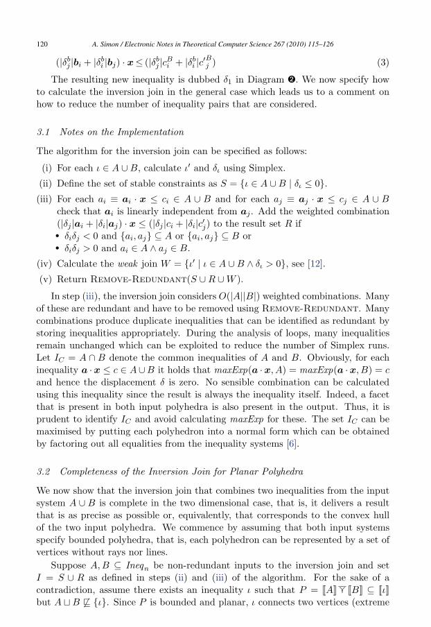
The resulting new inequality is dubbed δ1 in Diagram �. We now specify howto calculate the inversion join in the general case which leads us to a comment onhow to reduce the number of inequality pairs that are considered.

3.1 Notes on the Implementation

The algorithm for the inversion join can be specified as follows:

(i) For each ι ∈ A ∪ B, calculate ι′ and δι using Simplex.

(ii) Define the set of stable constraints as S = {ι ∈ A ∪ B | δι ≤ 0}.(iii) For each ai ≡ ai · x ≤ ci ∈ A ∪ B and for each aj ≡ aj · x ≤ cj ∈ A ∪ B

check that ai is linearly independent from aj . Add the weighted combination(|δj |ai + |δi|aj) · x ≤ (|δj |ci + |δi|c′j) to the result set R if• δiδj < 0 and {ai, aj} ⊆ A or {ai, aj} ⊆ B or• δiδj > 0 and ai ∈ A ∧ aj ∈ B.

(iv) Calculate the weak join W = {ι′ | ι ∈ A ∪ B ∧ δι > 0}, see [12].

(v) Return Remove-Redundant(S ∪ R ∪ W ).

In step (iii), the inversion join considers O(|A||B|) weighted combinations. Manyof these are redundant and have to be removed using Remove-Redundant. Manycombinations produce duplicate inequalities that can be identified as redundant bystoring inequalities appropriately. During the analysis of loops, many inequalitiesremain unchanged which can be exploited to reduce the number of Simplex runs.Let IC = A ∩ B denote the common inequalities of A and B. Obviously, for eachinequality a ·x ≤ c ∈ A∪B it holds that maxExp(a ·x, A) = maxExp(a ·x, B) = c

and hence the displacement δ is zero. No sensible combination can be calculatedusing this inequality since the result is always the inequality itself. Indeed, a facetthat is present in both input polyhedra is also present in the output. Thus, it isprudent to identify IC and avoid calculating maxExp for these. The set IC can bemaximised by putting each polyhedron into a normal form which can be obtainedby factoring out all equalities from the inequality systems [6].

3.2 Completeness of the Inversion Join for Planar Polyhedra

We now show that the inversion join that combines two inequalities from the inputsystem A ∪ B is complete in the two dimensional case, that is, it delivers a resultthat is as precise as possible or, equivalently, that corresponds to the convex hullof the two input polyhedra. We commence by assuming that both input systemsspecify bounded polyhedra, that is, each polyhedron can be represented by a set ofvertices without rays nor lines.

Suppose A, B ⊆ Ineqn be non-redundant inputs to the inversion join and setI = S ∪ R as defined in steps (ii) and (iii) of the algorithm. For the sake of acontradiction, assume there exists an inequality ι such that P = [[A]]� [[B]] ⊆ [[ι]]but A � B �� {ι}. Since P is bounded and planar, ι connects two vertices (extreme


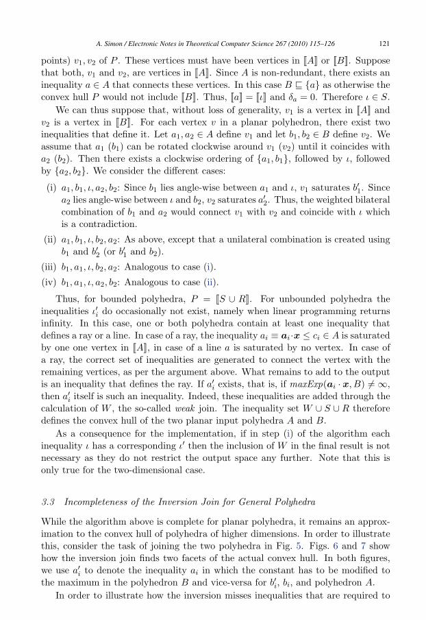
points) v1, v2 of P . These vertices must have been vertices in [[A]] or [[B]]. Supposethat both, v1 and v2, are vertices in [[A]]. Since A is non-redundant, there exists aninequality a ∈ A that connects these vertices. In this case B � {a} as otherwise theconvex hull P would not include [[B]]. Thus, [[a]] = [[ι]] and δa = 0. Therefore ι ∈ S.

We can thus suppose that, without loss of generality, v1 is a vertex in [[A]] andv2 is a vertex in [[B]]. For each vertex v in a planar polyhedron, there exist twoinequalities that define it. Let a1, a2 ∈ A define v1 and let b1, b2 ∈ B define v2. Weassume that a1 (b1) can be rotated clockwise around v1 (v2) until it coincides witha2 (b2). Then there exists a clockwise ordering of {a1, b1}, followed by ι, followedby {a2, b2}. We consider the different cases:

(i) a1, b1, ι, a2, b2: Since b1 lies angle-wise between a1 and ι, v1 saturates b′1. Sincea2 lies angle-wise between ι and b2, v2 saturates a′2. Thus, the weighted bilateralcombination of b1 and a2 would connect v1 with v2 and coincide with ι whichis a contradiction.

(ii) a1, b1, ι, b2, a2: As above, except that a unilateral combination is created usingb1 and b′2 (or b′1 and b2).

(iii) b1, a1, ι, b2, a2: Analogous to case (i).

(iv) b1, a1, ι, a2, b2: Analogous to case (ii).

Thus, for bounded polyhedra, P = [[S ∪ R]]. For unbounded polyhedra theinequalities ι′i do occasionally not exist, namely when linear programming returnsinfinity. In this case, one or both polyhedra contain at least one inequality thatdefines a ray or a line. In case of a ray, the inequality ai ≡ ai ·x ≤ ci ∈ A is saturatedby one one vertex in [[A]], in case of a line a is saturated by no vertex. In case ofa ray, the correct set of inequalities are generated to connect the vertex with theremaining vertices, as per the argument above. What remains to add to the outputis an inequality that defines the ray. If a′i exists, that is, if maxExp(ai · x, B) �= ∞,then a′i itself is such an inequality. Indeed, these inequalities are added through thecalculation of W , the so-called weak join. The inequality set W ∪ S ∪ R thereforedefines the convex hull of the two planar input polyhedra A and B.

As a consequence for the implementation, if in step (i) of the algorithm eachinequality ι has a corresponding ι′ then the inclusion of W in the final result is notnecessary as they do not restrict the output space any further. Note that this isonly true for the two-dimensional case.

3.3 Incompleteness of the Inversion Join for General Polyhedra

While the algorithm above is complete for planar polyhedra, it remains an approx-imation to the convex hull of polyhedra of higher dimensions. In order to illustratethis, consider the task of joining the two polyhedra in Fig. 5. Figs. 6 and 7 showhow the inversion join finds two facets of the actual convex hull. In both figures,we use a′i to denote the inequality ai in which the constant has to be modified tothe maximum in the polyhedron B and vice-versa for b′i, bi, and polyhedron A.

In order to illustrate how the inversion misses inequalities that are required to


x

y

a a

a

a

a

a

1

2

3

4

5

0

a5

a4

x

y

z

a3

a1a2

a0

❶ ❷

b

2

30va

bv

vava

bv

bv

bv

bv

bv

7vb

bv

1

2

3

4

5

6

0

b

b

b

bb b

1

2

3

4

5 6

0

1

2

3

0va

va

va

vabv

bv

bvbv

7vb

bv

1

3

4

5

6

bb b

b

02 5

6

Fig. 5. Polyhedron A, depicted as dark rectangle, is to be joined with pyramid B.

xy

z

b

b'

a

a'

4

5

5

4

v

v

a

b

0

1

7

vava

0

1va

vb1

�

vb7vb1

b4

a5

❶ ❷

Fig. 6. The relaxed constraints a′5 and b′4 are combined to the constraint δ.

a4

a'4

va1

vb0

vb2z

y

x

b1

a4

a'4

b'1

va1

vb0

vb2

b1

vb6

vb3

❶ ❷

�

vb1vb7vb1

vb7

a3

a5

Fig. 7. A weighted combination of inequalities a4 and b1.

define the exact convex hull of the input polyhedra, consider Fig. 8. Formally, thetask of calculating the convex hull of two polyhedra amounts to finding facets thatconnect a single vertex v of one polyhedron with a so-called horizon ridge of the otherpolyhedron. A ridge is the intersection of two adjacent facets, which, in turn, can beseen as the intersection of the boundaries of two inequalities ([[a·x = ca]]∩[[b·x = cb]]for inequalities a·x ≤ ca and b·x ≤ cb). A horizon ridge is formed by two inequalitiesof which one is “visible” from the vertex v while the other one is obscured, thatis, a · v �≤ ca indicates that the first facet is visible while b · v ≤ cb indicates


xy

z

❶ ❷ bv7vb

1

b1b3

3va

1va

a5

bv7vb

1

b1b3

3va

1va

a5

�2�1 w

a3a3

Fig. 8. The weighted combinations of a5, b1 and a5, b3 do not form a facet of the convex hull. The facet wwould be the most precise constraint but cannot be found by combining two inequalities.

that the second is obscured. The challenge in calculating the convex hull lies infinding ridges of a polyhedron. The inversion join combines two inequalities andoptimistically assumes that the result touches a ridge in one of the polyhedra. In thecase of b1 in � of Fig. 8, this assumption is wrong: In the diagram, the inequalitiesa5 and b1 are combined. While b1 forms a ridge with b3, b4 and b6; and a5 forms aridge with a0, . . . a3, the resulting inequality δ1 touches none of these ridges. Indeed,it connects a vertex to a vertex and is therefore redundant in the actual convex hull.On the contrary, the inversion join will miss opportunities to connect certain ridgesin a polyhedron to a vertex in the other polyhedron. This is illustrated in Diagram� of Fig. 8. Here, the ridge formed by a3, a5 could be connected to the vertex vb

1.However, since a′3 touches the vertex vb

2 rather than vertex vb1, this opportunity is

missed.We now present our prototype implementation and its evaluation.

4 Evaluation

The major challenge in implementing the inversion join in a sound way is the useof the Simplex solver. Since off-the-shelf solvers use floating-point arithmetic, theresult is not always correct. Thus, given c = maxExp(a·x, I), we discard the floatingpoint optimum c and query which inequalities IB ⊆ I the Simplex solver used asa basis when observing the maximum. We then find a vector λ of multipliers suchthat λA = a where IB ≡ Ax ≤ c. If c �= ∞ and no λ exists then the floating-pointsolver is wrong and we re-run the linear program using exact arithmetic which isabout 70 times slower.

We applied our implementation of the inversion join to a benchmark suite thatwas gathered in the context of the PIPS project [1] which pursued advanced opti-mizations and parallelization of Fortran code. The benchmarks [11] contain every100th input to the convex hull algorithm of the analyser while analyzing the Per-fect Club and Spec 95 Fortran benchmarks. The data in the benchmark consistof pairs of polyhedra that were joined during the analysis. Thus, the benchmarksonly contain few examples that are exponential as the analyzer would not haveprogressed after encountering a hard problem. Hence, there are no instance whereour algorithm delivers a result while the exact convex hull algorithm times out. We


dims. total # of incomplete join off by > 1 ineq. off by > 2 ineq.

(vars) test cases # of cases in % # of cases in % # of cases in %

2 848 0 0 0 0 0 0

3 574 62 11 9 2 4 1

4 340 60 18 25 7 7 2

5–6 586 167 28 104 18 64 11

7–8 344 134 39 87 25 77 22

9–11 296 189 64 161 54 143 48

12–17 225 134 60 123 55 112 50

18–32 238 175 74 168 71 159 67

≥ 33 41 17 41 17 41 15 37

≥ 2 3492 939 27 694 20 581 17

Table 1Performance of the join algorithm on a 2.4GHz Core 2 Linux computer.

generated a C++ program that calculates the convex hull of each test case using theParma Polyhedra Library [2] and a Haskell program that implements the inversionjoin, using the GNU Linear Programming Toolkit as solver [7]. The test programsrecord the results to disk which we used to count the number of inequalities thatthe inversion join lacks from the exact solution of the convex hull. The test resultsin Table 1 are partitioned by the number of dimensions (variables) in the outputpolyhedron except for the last row which shows the results for running all 3492tests. Next to the dimension we show the number of test cases and then three dou-ble columns that state how many of these test cases do not match the convex hull;those that lack at most one inequality and those that lack at most two. In eachdouble column the number of incomplete cases is given together with the percentageof the total. From the last row, it can be seen that the algorithm is exact in 73%of all cases and misses less than two inequalities in 83% of all cases. Note that thenumber of incomplete joins rises with the dimension which is to be expected as theconvex hull problem is exponential in the dimension.

5 Conclusion and Discussion

We assessed the precision of the inversion join in a qualitative and quantitative way.In particular, we argue that the inversion join with k = 2 is complete for planarpolyhedra. This begs the question if similar results are obtainable for k > 2. Thecompleteness in two dimensions implies that a TVPI system of inequalities can bejoined using the inversion join in a way that the result is more precise than thatof the TVPI domain. However, the result of applying the inversion join to a TVPI


system is not necessarily a TVPI system since inequalities may have more thantwo variables per inequality. Furthermore, widening, a process necessary to ensuretermination, is non-monotonic. Widening could therefore render an analysis usingthe inversion join less precise than that of the TVPI system. Further empiricalstudies that compare the precision of the two domains would thus be of interest.

On general polyhedra, our observation is that the inversion join produces verygood approximations to the precise convex hull algorithm while avoiding the ex-ponentially sized output cases. The inversion join therefore presents a sweetpointbetween precision and efficiency and we would argue for the inclusion of this algo-rithm into the common off-the-shelf polyhedra libraries.

The author wishes to thank Duong Nguyen Que for making the benchmark suiteavailable and also Liqian Chen for useful discussions. The author would also like tothank Antoine Mine for his diligent work as editor.

References

[1] Ancourt, C., F. Coelho, F. Irigoin and R. Keryell, A Linear Algebra Framework for Static HighPerformance Fortran Code Distribution, Scientific Programming 6 (1997), pp. 3–27.

[2] Bagnara, R., P. M. Hill and E. Zaffanella, Not Necessarily Closed Convex Polyhedra and the DoubleDescription Method, Formal Aspects of Computing 17 (2005), pp. 222–257.

[3] Cousot, P. and R. Cousot, Abstract Interpretation and Application to Logic Programs, Journal of LogicProgramming 13 (1992), pp. 103–179.

[4] Cousot, P. and N. Halbwachs, Automatic Discovery of Linear Constraints among Variables of aProgram, in: Principles of Programming Languages (1978), pp. 84–97.

[5] Howe, J. M. and A. King, Logahedra: a New Weakly Relational Domain, in: Z. Lu and A. P. Ravn,editors, Automated Technology for Verification and Analysis, LNCS (2009).

[6] Lassez, J.-L. and K. McAloon, A Canonical Form for Generalized Linear Constraints, Journal ofSymbolic Computation 13 (1993), pp. 1–24.

[7] Makhorin, A., GLPK (GNU Linear Programming Kit) (2008), version 4.32.URL http://www.gnu.org/software/glpk/

[8] Mauborgne, L. and X. Rival, Trace Partitioning in Abstract Interpretation Based Static Analyzers, in:M. Sagiv, editor, European Symposium on Programming, LNCS 3444 (2005), pp. 5–20.

[9] Mine, A., The Octagon Abstract Domain, Higher-Order and Symbolic Computation 19 (2006), pp. 31–100.

[10] Mine, A., Symbolic Methods to Enhance the Precision of Numerical Abstract Domains, in: E. A.Emerson and K. S. Namjoshi, editors, Verification, Model Checking and Abstract Interpretation, LNCS3855 (2006), pp. 348–363.

[11] Nguyen-Que, D., Polybench (2006).URL http://www.cri.ensmp.fr/people/duong/polybench

[12] Sankaranarayanan, S., M. Colon, H. B. Sipma and Z. Manna, Efficient Strongly Relational PolyhedralAnalysis., in: E. A. Emerson and K. S. Namjoshi, editors, Verification, Model Checking and AbstractInterpretation, LNCS 3855 (2006), pp. 111–125.

[13] Sankaranarayanan, S., H. B. Sipma and Z. Manna, Scalable Analysis of Linear Systems UsingMathematical Programming, in: R. Cousot, editor, Verification, Model Checking, and AbstractInterpretation, LNCS 3385 (2005), pp. 25–41.

[14] Simon, A., Splitting the Control Flow with Boolean Flags, in: M. Alpuente and G. Vidal, editors, StaticAnalysis Symposium, LNCS 5079 (2008), pp. 315–331.


http://www.gnu.org/software/glpk/

http://www.cri.ensmp.fr/people/duong/polybench

[15] Simon, A. and A. King, Exploiting Sparsity in Polyhedral Analysis, in: C. Hankin and I. Siveroni,editors, Static Analysis Symposium, LNCS 3672 (2005), pp. 336–351.

[16] Simon, A., A. King and J. M. Howe, Two Variables per Linear Inequality as an Abstract Domain,in: M. Leuschel, editor, Logic-Based Program Synthesis and Transformation, LNCS 2664 (2003), pp.71–89.


Documents

A Note on the Inversion Join for Polyhedral Analysis