Embed Size (px)
Citation preview

A note on concave utility functions1
Martin Monti
Princeton University
Simon Grant
Rice University
Daniel Osherson
Princeton University
April 1, 2004
1Contact information: M. Monti, Dept. of Psychology, Green Hall, Princeton Univer-sity, Princeton NJ 08544. Fax: 609-258-1113. Electronic mail: [email protected],[email protected], [email protected].
Abstract
The classical theory of preference among monetary bets represents people as expected
utility maximizers with nondecreasing concave utility functions. Critics of this account
often rely on assumptions about preferences over wide ranges of total wealth. We
derive a prediction of the theory that bears on bets at any fixed level of wealth, and
test the prediction behaviorally. Our results are discrepant with the classical account.
Competing theories are also examined in light of our data.
JEL classification: D81, C91.
keywords: gambling, risk aversion, concave utility function, expected utility, prospect
theory
A note on concave utility functions 1
An influential theory of preferences among bets represents people as expected utility
maximizers with nondecreasing concave utility functions. In what follows, we shall call
anyone who behaves this way a classical agent. The theory that people behave towards
bets as if they were classical agents has been the subject of intense discussion, with
alternative hypotheses prompted by experimental findings at variance with the classical
account.1 A new kind of objection has recently been formulated by Rabin (2000a,b;
Rabin & Thaler, 2001). Let (g, p, `) denote the bet yielding gain $g with probability
p and loss $` with probability 1− p. Rabin deduces predictions of the form:
A classical agent who declines bet (g, p, `) at wealth levels within interval
I will decline bet (g′, p′, `′) at wealth level J .
For example, he shows that:
(a) A classical agent who declines (110, .5, 100) at all wealth levels will decline
(X, .5, 1000) for every X and every wealth level.
(b) A classical agent who declines (105, .5, 100) through wealth level $350,000 will
decline (635670, .5, 4000) at wealth level $340,000.
These predictions are all the more remarkable for being “parameter free.” No assump-
tions about the utility curve are made except for its concavity throughout the domain
of money. Rabin believes that the predictions do not conform to typical human pref-
erences, hence most people are not classical agents. Indeed, Rabin & Thaler (2001)
conclude that the classical theory corresponds to the dead parrot in the famous sketch
from Monty Python’s Flying Circus, and they “aspire to have written one of the last
articles debating the descriptive validity of the expected utility hypothesis” (p. 229).
Not everyone, however, acknowledges the infidelity of (a),(b) to human preferences.
Watt (2002) and Palacios-Huerta, Serrano & Volij (2002), for example, observe that
the antecedent of (a) is difficult to verify empirically since it involves imagining choices
under counterfactual circumstances of immense wealth. Prediction (b) is more tren-
chant in this regard, but it is not clear (pace the intuitions of Rabin and Thaler) what
most people would do at the cited wealth levels. In particular, for someone as risk
averse as indicated in the premise of (b), a $4,000 loss might be a fearsome prospect
when her fortune is limited to $340,000.2
The present note attempts to preserve the spirit of Rabin’s criticism while avoiding
assumptions about behaviors across a wide range of wealth. We deduce a prediction
about the choices of classical agents at a given level of wealth, and then present ex-
perimental evidence contrary to the prediction. Defects in the classical theory have
A note on concave utility functions 2
been revealed in many experiments (e.g., the probability of choosing a given option
can be increased by adding a new one; see Huber, Payne & Puto, 1982; Simonson &
Tversky, 1992; Tentori, Osherson, Hasher & May, 2001). The present demonstration
is distinctive in its simplicity, and in its focus on the supposed concavity of the utility
function.
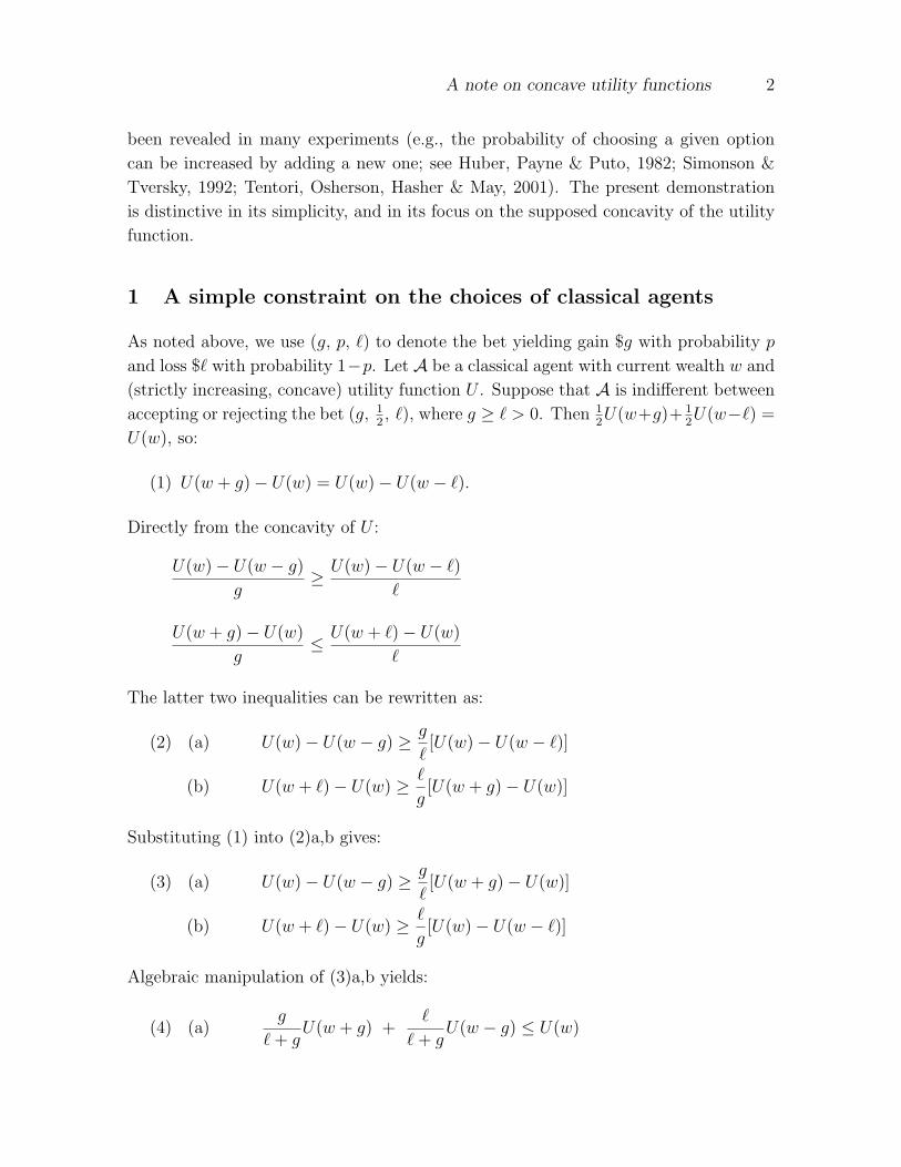
1 A simple constraint on the choices of classical agents
As noted above, we use (g, p, `) to denote the bet yielding gain $g with probability p
and loss $` with probability 1−p. Let A be a classical agent with current wealth w and
(strictly increasing, concave) utility function U . Suppose that A is indifferent between
accepting or rejecting the bet (g, 12, `), where g ≥ ` > 0. Then 1
2U(w+g)+ 1
2U(w−`) =
U(w), so:
(1) U(w + g)− U(w) = U(w)− U(w − `).
Directly from the concavity of U :
U(w)− U(w − g)
g≥ U(w)− U(w − `)
`
U(w + g)− U(w)
g≤ U(w + `)− U(w)
`
The latter two inequalities can be rewritten as:
(2) (a) U(w)− U(w − g) ≥ g
`[U(w)− U(w − `)]
(b) U(w + `)− U(w) ≥ `
g[U(w + g)− U(w)]
Substituting (1) into (2)a,b gives:
(3) (a) U(w)− U(w − g) ≥ g
`[U(w + g)− U(w)]
(b) U(w + `)− U(w) ≥ `
g[U(w)− U(w − `)]
Algebraic manipulation of (3)a,b yields:
(4) (a)g
` + gU(w + g) +
`
` + gU(w − g) ≤ U(w)
A note on concave utility functions 3
(b)g
` + gU(w + `) +
`
` + gU(w − `) ≥ U(w)
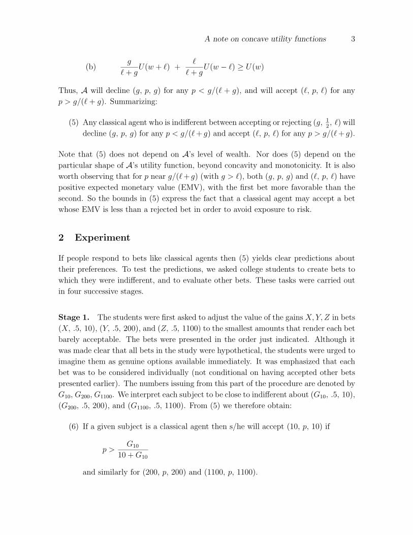
Thus, A will decline (g, p, g) for any p < g/(` + g), and will accept (`, p, `) for any
p > g/(` + g). Summarizing:
(5) Any classical agent who is indifferent between accepting or rejecting (g, 12, `) will
decline (g, p, g) for any p < g/(`+ g) and accept (`, p, `) for any p > g/(`+ g).
Note that (5) does not depend on A’s level of wealth. Nor does (5) depend on the
particular shape of A’s utility function, beyond concavity and monotonicity. It is also
worth observing that for p near g/(`+ g) (with g > `), both (g, p, g) and (`, p, `) have
positive expected monetary value (EMV), with the first bet more favorable than the
second. So the bounds in (5) express the fact that a classical agent may accept a bet
whose EMV is less than a rejected bet in order to avoid exposure to risk.
2 Experiment
If people respond to bets like classical agents then (5) yields clear predictions about
their preferences. To test the predictions, we asked college students to create bets to
which they were indifferent, and to evaluate other bets. These tasks were carried out
in four successive stages.
Stage 1. The students were first asked to adjust the value of the gains X,Y, Z in bets
(X, .5, 10), (Y, .5, 200), and (Z, .5, 1100) to the smallest amounts that render each bet
barely acceptable. The bets were presented in the order just indicated. Although it
was made clear that all bets in the study were hypothetical, the students were urged to
imagine them as genuine options available immediately. It was emphasized that each
bet was to be considered individually (not conditional on having accepted other bets
presented earlier). The numbers issuing from this part of the procedure are denoted by
G10, G200, G1100. We interpret each subject to be close to indifferent about (G10, .5, 10),
(G200, .5, 200), and (G1100, .5, 1100). From (5) we therefore obtain:
(6) If a given subject is a classical agent then s/he will accept (10, p, 10) if
p >G10
10 + G10
and similarly for (200, p, 200) and (1100, p, 1100).
A note on concave utility functions 4
Stage 2. Next, each participant adjusted the losses X,Y, Z in bets (10, .5, X),
(200, .5, Y ), and (1100, .5, Z) to the largest amounts that render each bet barely
acceptable (bets presented in the order indicated). The numbers issuing from this part
of the procedure are denoted by L10, L200, L1100. We interpret each subject to be close
to indifferent about (10, .5, L10), (200, .5, L200), and (1100, .5, L1100). From (5) we
therefore obtain:
(7) If a given subject is a classical agent then s/he will decline (10, p, 10) if
p <10
L10 + 10
and similarly for (200, p, 200) and (1100, p, 1100).
Stage 3. Participants were then asked whether they would accept each bet in a series
of twelve. The twelve bets were presented in random order, and a yes/no decision was
made to each in turn. Six of the bets were “fillers,” designed to mask the focus of the
experiment. The other six had the following forms.
(8)
a) (10, p, 10) where p = .95× (10/(L10 + 10))
b) (200, p, 200) where p = .95× (200/(L200 + 200))
c) (1100, p, 1100) where p = .95× (1100/(L1100 + 1100))
d) (10, p, 10) where p = 1.05× (G10/(G10 + 10))
e) (200, p, 200) where p = 1.05× (G200/(G200 + 200))
f) (1100, p, 1100) where p = 1.05× (G1100/(G1100 + 1100))
Thus, if our participants were classical agents, (6) and (7) predict that they decline
bets (8)a,b,c and accept bets (8)d,e,f. Note our use of probabilities that fall decisively
on the active side of each boundary (either 95% of the highest unacceptable probability
or 105% of the least acceptable one).
Stage 4. Finally, for each of three bets of form (x, p, x), participants were asked to
specify the minimum probability p that renders (x, p, x) barely acceptable. The three
bets were (10, p, 10), (200, p, 200), (1100, p, 1100), evaluated in that order. According
to (6) and (7), the value of p chosen for the three bets should lie in the following
intervals.
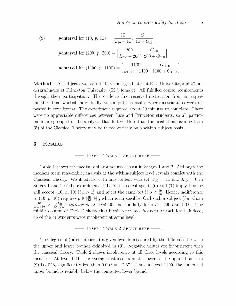
A note on concave utility functions 5
(9) p-interval for (10, p, 10) =[
10
L10 + 10,
G10
10 + G10
]
p-interval for (200, p, 200) =[
200
L200 + 200,
G200
200 + G200
]
p-interval for (1100, p, 1100) =[
1100
L1100 + 1100,
G1100
1100 + G1100
]
Method. As subjects, we recruited 23 undergraduates at Rice University, and 28 un-
dergraduates at Princeton University (52% female). All fulfilled course requirements
through their participation. The students first received instruction from an exper-
imenter, then worked individually at computer consoles where instructions were re-
peated in text format. The experiment required about 20 minutes to complete. There
were no appreciable differences between Rice and Princeton students, so all partici-
pants are grouped in the analyses that follow. Note that the predictions issuing from
(5) of the Classical Theory may be tested entirely on a within subject basis.
3 Results
——- Insert Table 1 about here ——-
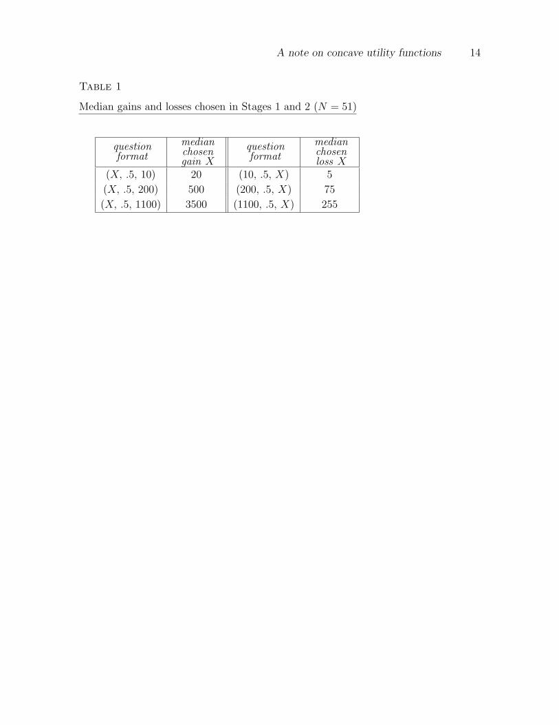
Table 1 shows the median dollar amounts chosen in Stages 1 and 2. Although the
medians seem reasonable, analysis at the within-subject level reveals conflict with the
Classical Theory. We illustrate with one student who set G10 = 11 and L10 = 6 in
Stages 1 and 2 of the experiment. If he is a classical agent, (6) and (7) imply that he
will accept (10, p, 10) if p > 1121
and reject the same bet if p < 1016
. Hence, indifference
to (10, p, 10) requires p ∈ [1016
, 1121
], which is impossible. Call such a subject (for whom10
L10+10> G10
10+G10) incoherent at level 10, and similarly for levels 200 and 1100. The
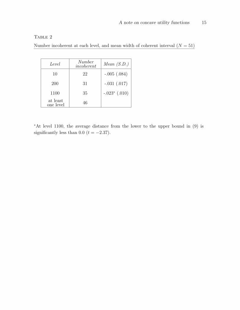
middle column of Table 2 shows that incoherence was frequent at each level. Indeed,
46 of the 51 students were incoherent at some level.
——- Insert Table 2 about here ——-
The degree of (in)coherence at a given level is measured by the difference between
the upper and lower bounds exhibited in (9). Negative values are inconsistent with
the classical theory. Table 2 shows incoherence at all three levels according to this
measure. At level 1100, the average distance from the lower to the upper bound in
(9) is -.023, significantly less than 0.0 (t = −2.37). Thus, at level 1100, the computed
upper bound is reliably below the computed lower bound.
A note on concave utility functions 6
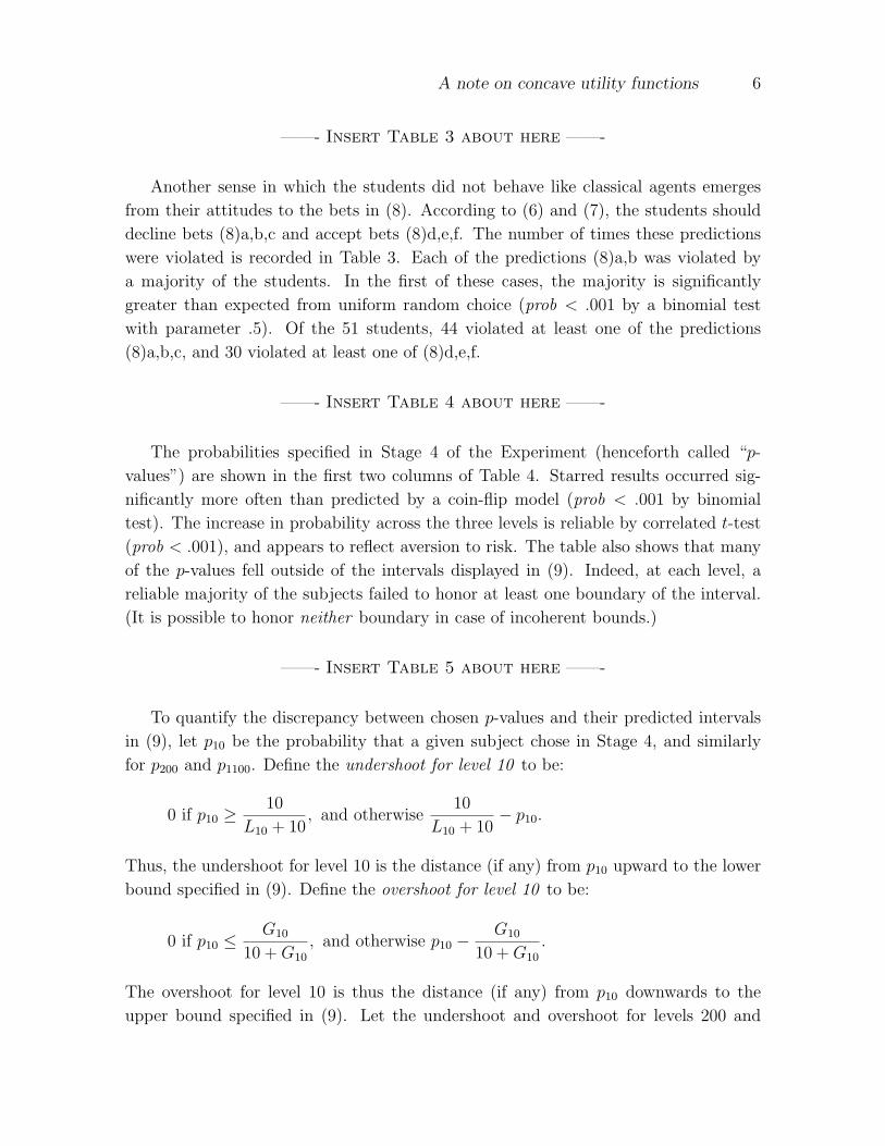
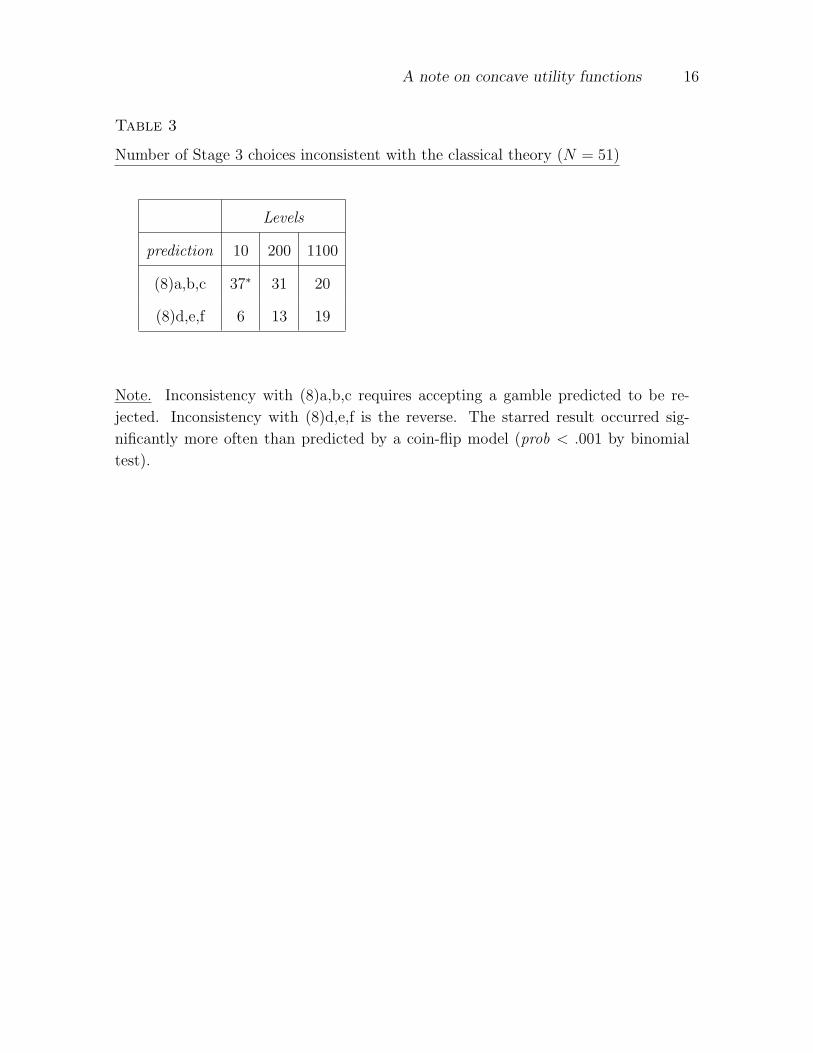
——- Insert Table 3 about here ——-
Another sense in which the students did not behave like classical agents emerges
from their attitudes to the bets in (8). According to (6) and (7), the students should
decline bets (8)a,b,c and accept bets (8)d,e,f. The number of times these predictions
were violated is recorded in Table 3. Each of the predictions (8)a,b was violated by
a majority of the students. In the first of these cases, the majority is significantly
greater than expected from uniform random choice (prob < .001 by a binomial test
with parameter .5). Of the 51 students, 44 violated at least one of the predictions
(8)a,b,c, and 30 violated at least one of (8)d,e,f.
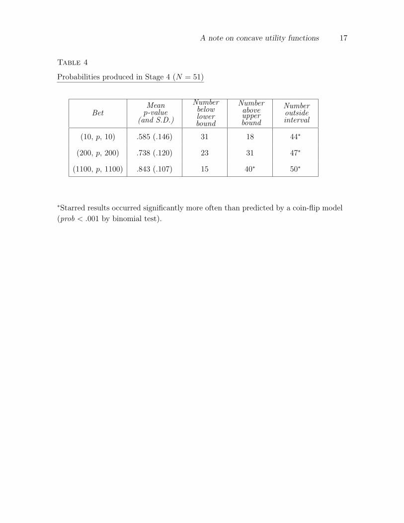
——- Insert Table 4 about here ——-
The probabilities specified in Stage 4 of the Experiment (henceforth called “p-
values”) are shown in the first two columns of Table 4. Starred results occurred sig-
nificantly more often than predicted by a coin-flip model (prob < .001 by binomial
test). The increase in probability across the three levels is reliable by correlated t-test
(prob < .001), and appears to reflect aversion to risk. The table also shows that many
of the p-values fell outside of the intervals displayed in (9). Indeed, at each level, a
reliable majority of the subjects failed to honor at least one boundary of the interval.
(It is possible to honor neither boundary in case of incoherent bounds.)
——- Insert Table 5 about here ——-
To quantify the discrepancy between chosen p-values and their predicted intervals
in (9), let p10 be the probability that a given subject chose in Stage 4, and similarly
for p200 and p1100. Define the undershoot for level 10 to be:
0 if p10 ≥10
L10 + 10, and otherwise
10
L10 + 10− p10.
Thus, the undershoot for level 10 is the distance (if any) from p10 upward to the lower
bound specified in (9). Define the overshoot for level 10 to be:
0 if p10 ≤G10
10 + G10
, and otherwise p10 −G10
10 + G10
.
The overshoot for level 10 is thus the distance (if any) from p10 downwards to the
upper bound specified in (9). Let the undershoot and overshoot for levels 200 and
A note on concave utility functions 7
1100 be defined similarly. Table 5 shows the undershoots and overshoots at each level.
Thus, the average distance from p10 upward to the lower bound for (10, p, 10) shown
in (9) is .076 (S.D. = .099). (If p10 for a given subject is above the bound then his/her
contribution to the mean is zero.) The average distance from p10 downward to the upper
bound for (10, p, 10) shown in (9) is .027 (S.D. = .050). (If p10 for a given subject is
below the bound then his/her contribution to the mean is zero.) The other numbers in
Table 5 are interpreted similarly. The table shows that the undershoots were greater
for level 10 compared to 200, and greater for 200 compared to 1100; likewise, the
overshoots were greater for level 1100 compared to 200, and for 200 compared to 10.
All the means differ reliably from each other (prob < .02) by correlated t-test except for
the undershoots at levels 200 and 1100 (t = 1.78), and the undershoot versus overshoot
at level 200 (t = 1.69). It is thus clear that the participants deviated from classical
agents in a systematic rather than random way.
Call a subject classical at level 10 if her p-value for that level lies in the (coherent)
p-interval[
10L10+10
, G10
10+G10
], and similarly for levels 200 and 1100. Only 7 subjects were
classical at level 10, 4 at level 200, and 1 at level 1100. Not a single subject behaved
like a classical agent at all three levels.
4 Alternatives to the classical theory
Consider again an agent A whose preferences among bets are governed by nondecreas-
ing utility curve U . Suppose that A is indifferent between accepting and rejecting the
bet (g, .5, `), where g ≥ ` > 0. Then 12U(w + g) + 1
2U(w− `) = U(w), and once again
we obtain equality (1), repeated here:
(1) U(w + g)− U(w) = U(w)− U(w − `).
If U is concave (respectively, convex) in the domain of gains then:
U(w + g)− U(w)
g≤ (respectively, ≥ )
U(w + `)− U(w)
`
These inequalities concern the “domain of gains” because only increases to w are at
issue. Similarly, if U is concave (respectively, convex) in the domain of losses then:
U(w)− U(w − g)
g≥ (respectively, ≤ )
U(w)− U(w − `)
`
A note on concave utility functions 8
Substituting (1) into the latter inequalities produces:
U(w + `)− U(w) ≥ (respectively, ≤ )`
g[U (w)− U (w − `)]
U(w)− U(w − g) ≥ (respectively, ≤ )g
`[U(w + g)− U(w)]
Algebraic manipulation then yields the following.
(10) (a) If U is concave (respectively, convex) in the domain of gains then:
g
` + gU (w + `) +
`
` + gU (w − `) ≥ (respectively, ≤ ) U (w)
(b) If U is concave (respectively, convex) in the domain of losses then:
g
` + gU (w + g) +
`
` + gU (w − g) ≤ (respectively, ≥ ) U (w)
If U is concave in both the domain of gains and the domain of losses then we
recover our classical agent, described by (5). If U is concave in the domain of gains
and convex in the domain of losses then A resembles the kind of agent depicted in
Prospect Theory (Kahneman & Tversky, 1978). In this case, (10) implies that Awill accept both (g, p, g) and (`, p, `) if p > g/(` + g). [Hence, the probability that Aassigns in Stage 4 of the experiment must lie below X/(LX +X) and GX/(X +GX), for
each level X ∈ {10, 200, 1100}.] In contrast, if U is convex in the domain of gains and
concave in the domain of losses then A is more like the agent discussed by Friedman &
Savage (1948). In this case, (10) implies that A will decline both (g, p, g) and (`, p, `)
if p < g/(` + g). [Hence, the probability that A assigns in Stage 4 of the experiment
must lie above X/(LX + X) and GX/(X + GX), for each level X ∈ {10, 200, 1100}.]Let us introduce the following terminology.
(11) Definition: Let X ∈ {10, 200, 1100} be given. Let GX and LX be the values
assigned in Stages 1 and 2 of the experiment, and let pX be the probability
assigned in Stage 4.
(a) A subject is KT at level X if and only if pX bounded above by both
X/(LX + X) and GX/(X + GX). (KT abbreviates “Kahneman & Tver-
sky”.)
(b) A subject is FS at level X if and only if pX is bounded below by both
X/(LX + X) and GX/(X + GX). (FS abbreviates “Friedman & Savage”.)
A note on concave utility functions 9
The definition provides apt characterizations of Kahneman & Tversky (1978) and Fried-
man & Savage (1948) only if
(12) GX ≥ X ≥ LX and pX ≥ .5
inasmuch as these inequalities were assumed for the developments above. In what
follows, at each level X we therefore exclude subjects who violated (12).
Consider a subject S who satisfies (12). The weak inequalities appearing in Defini-
tion (11) allow S to be more than one of KT, FS, and classical. It is also possible for S
to be none of the three types. For example, one subject (mentioned at the beginning
of the Results section) chose G10 = 11, L10 = 6, p10 = .55; calculation of 10/(L10 + 10)
and G10/(X +G10) reveals that .55 is neither above both these bounds (thus ruling out
FS), nor below both (ruling out KT), nor “in between” (since the bounds are inverted,
which rules out classical).
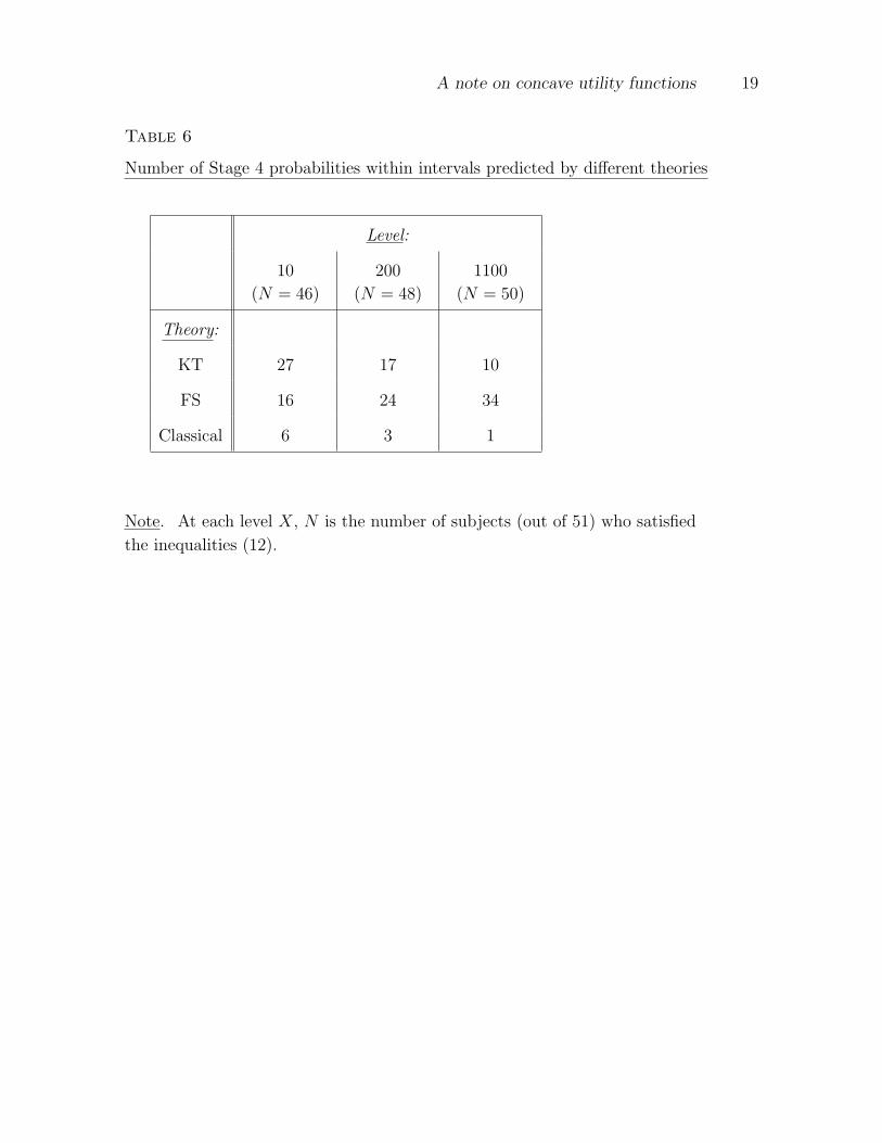
——- Insert Table 6 about here ——-
Table 6 shows the number of subjects of each kind (KT, FS, classical) at the three
levels. It also exhibits the number of subjects (out of 51) conforming to (12). At
each level, a large majority is either KT or FS; few are classical. The difference in
proportions of KT and classical subjects is reliable at each level (prob < .01); the same
is true of the differences between FS and classical subjects. There were reliably more
KT than FS subjects at level 10 (prob < .02), and the reverse at level 1100 (prob < .01);
there is no reliable difference at level 200.
A different alternative to the classical theory posits “first-order” aversion to risk,
that is, the disinclination to accept fair gambles even with tiny stakes; in contrast,
classical agents are indifferent to them; see Segal & Spivak (1990). In an influential
article, Gul (1991) offers a generalization of utility theory that is consistent with first-
order aversion. It implies that an agent with wealth w and utility function U will
accept (g, p, `) if and only if
(13) U(w) < Uw(g, p, `) =p
p + (1− p)λU(w + g) +
(1− p)λ
p + (1− p)λU(w − `),
where λ is a parameter characterizing the agent’s aversion to disappointment; the
standard theory is recovered at λ = 1. It follows easily that for any level w of wealth,
the marginal change in Uw(ε, .5, ε) goes to 1−λ1+λ
U ′(w) as ε → 0, signifying first-order
aversion to loss when λ > 1.
A note on concave utility functions 10
If Gul’s model is descriptively accurate with concave U , it might be taken as partial
vindication of the classical theory. To investigate this possibility, call an agent Gul if
her preferences for gambles are governed by inequality (13), where U is concave and
λ > 0. By an argument similar to the one advanced earlier, we can show:
Any Gul agent who is indifferent between accepting or rejecting (g, 12, `)
will decline (g, p, g) for any p < g/(` + g) and accept (`, p, `) for any
p > g/(` + g).
Since this is the same prediction as (5) for classical agents, our experimental results
conflict with (13) as much as they conflict with the classical theory. It therefore appears
that adding first-order risk-aversion to the concavity assumption may not be sufficient
to describe real choices among lotteries.
5 Discussion
The experimental results are discrepant with the hypothesis that college students be-
have like classical agents when evaluating bets. Instead of behaving classically, Table
6 suggests that at low stakes, most subjects choose as if their utility for money were
concave for gains and convex for losses (as suggested by Kahneman & Tversky, 1978);
the reverse patterns holds for high stakes (conforming to Friedman & Savage, 1948).
The discrepancy with the classical theory thus appears to be systematic.3
Two caveats must be entered. First, the bets in our study were hypothetical so it
remains possible that the students would respond like classical agents if faced with the
real thing.4 Second, people might resemble classical agents better when they are led to
conceptualize bets in terms of overall wealth, e.g., in terms of U(w− $10) rather than
a decontextualized $10 loss. It is well known that attitudes towards gains versus losses
are asymmetric in ways that apply less to overall wealth.5
The results nonetheless suggest that the classical theory of risk aversion is qualita-
tively inaccurate. For, choices deviate in systematic fashion from predictions that are
independent of parametric assumptions about the utility curve, beyond concavity itself.
In this sense, our findings sustain the principal thesis advanced in Rabin (2000a,b).
A note on concave utility functions 11
Notes
1See Kahneman & Tversky (2000) for assessment of the descriptive realism of utility
theory, and alternative models. For a history of the classical theory, see Arrow (1971);
its success in behavioral prediction is reviewed in Camerer (1995).
2LeRoy (2003) offers reason to doubt that most people reject small, unfavorable
gambles like (105, .5, 100). But see Rabin & Thaler’s (2002) response to critics, and
the data they cite about risk aversion in gambles with small stakes.
3Since gambles were always evaluated in order of increasing stakes — 10 to 200 to
1100 — the apparent interaction between stakes and conformity to KT versus FS may
be partly an order effect.
4The impact of real stakes on conformity to economic postulates, however, is not
straightforward. See Camerer & Hogarth (1999) for a review of findings.
5See Tversky & Bar-Hillel (1983), Kahneman, Knetsch & Thaler (1991), Kahneman
& Tversky (1995), and references cited there.
A note on concave utility functions 12
References
Arrow, Kenneth J. (1971) Essays in the Theory of Risk Bearing (Chicago IL:
Markham Publishing Company)
Camerer, Colin (1995) ‘Individual Decision Making.’ In Handbook of Experimental
Economics, ed. John Kagel and Al Roth (Princeton NJ: Princeton University Press)
Camerer, Colin, and Robin Hogarth (1999) ‘The effects of financial incentives in
economic experiments: A review and capital-labor-production framework.’ Journal
of Risk and Uncertainty 18, 7–42
Friedman, Milton, and Leonard Savage (1948) ‘The utility analysis of choices
involving risk.’ Journal of Political Economy 56(4), 279–304
Gul, Faruk (1991) ‘A theory of disappointment aversion.’ Econometrica
59(3), 667–686
Huber, Joel, John W. Payne, and Chris Puto (1982) ‘Adding asymmetrically
dominated alternatives: violations of regularity and the similarity hypothesis.’
Journal of Consumer Research 9, 90–98
Kahneman, Daniel, and Amos Tversky (1979) ‘Prospect Theory: An Analysis of
Decision under Risk.’ Econometrica 47(2), 263–91
(1995) ‘Conflict Resolution: A Cognitive Perspective.’ In Barriers to Conflict
Resolution, ed. Kenneth J. Arrow (New York NY: W.W. Norton)
Kahneman, Daniel, and Amos Tversky, eds (2000) Choices, Values, and Frames
(Cambridge, England: Cambridge University Press)
Kahneman, Daniel, John L. Knetsch, and Richard Thaler (1991) ‘Anomalies: The
Endowment Effect, Loss Aversion, and Status Quo Bias.’ Journal of Economic
Perspectives 5(1), 193–206
LeRoy, Stephen (2003) ‘Expected utility: a defense.’ Economics Bulletin 7(7), 1–3
Palacios-Huerta, Ignacio, Robert Serrano, and Oscar Volij (2002) ‘Rejecting Small
Gambles Under Epected Utility.’ Manuscript
Pratt, John (1964) ‘Risk Aversion in the Small and in the Large.’ Econometrica
32, 122–136
Rabin, M. (2000a) ‘Risk Aversion and Expected-Utility: A Calibration Theorem.’
Econometrica 68, 1281–1292
Rabin, M., and R. Thaler (2001) ‘Risk aversion.’ Journal of Economic Perspectives
15, 219–232
Rabin, Matthew (2000b) ‘Diminishing Marginal Utility of Wealth Cannot Explain
Risk Aversion.’ In Choices, Values, and Frames, ed. Daniel Kahneman and Amos
Tversky (Cambridge, England: Cambridge University Press)
Rabin, Matthew, and Richard Thaler (2002) ‘Response.’ Journal of Economic
A note on concave utility functions 13
Perspectives 16(2), 229–230
Segal, Uzi, and Avia Spivak (1990) ‘First-order versus second-order risk aversion.’
Journal of Economic Theory 51, 111–125
Simonson, Israel, and Amos Tversky (1992) ‘Choice in context: Tradeoff contrast and
extremeness aversion.’ Journal of Marketing Research 29, 281–287
Tentori, Katya, Daniel Osherson, Lynn Hasher, and Cynthia May (2001) ‘Wisdom
and aging: Irrational preferences in college students but not older adults.’
Cognition 81/3, B87–B96
Tversky, Amos, and Maya Bar-Hillel (1983) ‘Risk: The Long and the Short.’ Journal
of Experimental Psychology: Learning, Memory and Cognition 9(4), 713–117
Watt, Richard (2002) ‘Defending expected utility theory.’ Journal of Economic
Perspectives 16(2), 227–230
A note on concave utility functions 14
Table 1
Median gains and losses chosen in Stages 1 and 2 (N = 51)
questionformat
medianchosengain X
questionformat
medianchosenloss X
(X, .5, 10) 20 (10, .5, X) 5
(X, .5, 200) 500 (200, .5, X) 75
(X, .5, 1100) 3500 (1100, .5, X) 255
A note on concave utility functions 15
Table 2
Number incoherent at each level, and mean width of coherent interval (N = 51)
Level Numberincoherent Mean (S.D.)
10 22 -.005 (.084)
200 31 -.031 (.017)
1100 35 -.023∗ (.010)
at leastone level 46
∗At level 1100, the average distance from the lower to the upper bound in (9) is
significantly less than 0.0 (t = −2.37).
A note on concave utility functions 16
Table 3
Number of Stage 3 choices inconsistent with the classical theory (N = 51)
Levels
prediction 10 200 1100
(8)a,b,c 37∗ 31 20
(8)d,e,f 6 13 19
Note. Inconsistency with (8)a,b,c requires accepting a gamble predicted to be re-
jected. Inconsistency with (8)d,e,f is the reverse. The starred result occurred sig-
nificantly more often than predicted by a coin-flip model (prob < .001 by binomial
test).
A note on concave utility functions 17
Table 4
Probabilities produced in Stage 4 (N = 51)
BetMean
p-value(and S.D.)
Numberbelowlowerbound
Numberaboveupperbound
Numberoutsideinterval
(10, p, 10) .585 (.146) 31 18 44∗
(200, p, 200) .738 (.120) 23 31 47∗
(1100, p, 1100) .843 (.107) 15 40∗ 50∗
∗Starred results occurred significantly more often than predicted by a coin-flip model
(prob < .001 by binomial test).

A note on concave utility functions 18
Table 5
Undershoot and overshoot in Stage 4 (N = 51)
BetMean
undershoot(and S.D.)
Meanovershoot(and S.D.)
(10, p, 10) .076 (.099) .027 (.050)
(200, p, 200) .032 (.049) .061 (.099)
(1100, p, 1100) .011 (.029) .093 (.088)
A note on concave utility functions 19
Table 6
Number of Stage 4 probabilities within intervals predicted by different theories
Level:
10
(N = 46)
200
(N = 48)
1100
(N = 50)
Theory:
KT 27 17 10
FS 16 24 34
Classical 6 3 1
Note. At each level X, N is the number of subjects (out of 51) who satisfied
the inequalities (12).