HAL Id: hal-02079224https://hal.archives-ouvertes.fr/hal-02079224

Preprint submitted on 25 Mar 2019

HAL is a multi-disciplinary open accessarchive for the deposit and dissemination of sci-entific research documents, whether they are pub-lished or not. The documents may come fromteaching and research institutions in France orabroad, or from public or private research centers.

L’archive ouverte pluridisciplinaire HAL, estdestinée au dépôt et à la diffusion de documentsscientifiques de niveau recherche, publiés ou non,émanant des établissements d’enseignement et derecherche français ou étrangers, des laboratoirespublics ou privés.

A New Sine-G Family of Distributions: Properties andApplications

Zafar Mahmood, Christophe Chesneau

To cite this version:Zafar Mahmood, Christophe Chesneau. A New Sine-G Family of Distributions: Properties and Ap-plications. 2019. �hal-02079224�

1

A New Sine-G Family of Distributions:

Properties and Applications

Zafar Mahmood1 and Christophe Chesneau2

Abstract: This paper is devoted to the study of a new family of distributions basedon a sine transformation. In some situations, we show that the new family providesa suitable alternative to the so-called sine-G family of distributions, with the samenumber of parameters. Among others, some of its significant mathematical proper-ties are derived, including shapes of probability density and hazard rate functions,asymptotes, quantile function, useful expansions, moments and moment generatingfunction. Then, a special member with two parameters, using the inverse Weibulldistribution as baseline, is introduced and investigated in detail. By consideringthis new distribution as a statistical model, the parameters are estimated via themaximum likelihood method. A simulation study is carried out to assess the per-formance of the obtained estimators. The applications on two real data sets areexplored, showing the ability of the proposed model to fit various type of data sets.

Key words and phrases: Trigonometric distributions; Moments; Weibull distribu-tion; Real life data sets.

AMS 2000 Subject Classifications: 62G05, 62G20.

1 Introduction

A challenging work for the statistician is to construct flexible models for modelling various typesof data. Generally, this allows to reveal new features of real life phenomena and provide advisedpredictions. In this regards, numerous families of distributions have been created via varioustechniques (differential equations, induction of location, scale, shape parameters, compounding,weighting . . . ), each giving flexible models, with specific properties. Among the most usefulfamilies of distributions, there are the Marshall-Olkin-G family introduced by [17], the exp-Gfamily introduced by [9], the beta-G family introduced by [7], the gamma-G family developedby [28], the RB-G family introduced by [23], the TX-G family introduced by [2], the Weibull-Gfamily developed by [5], the sine-G family introduced by [15] and the generalized odd Gamma-Gfamily introduced by [10].

This study proposes a new family of distributions following the spirit of the sine-G family.A brief description of the sine-G family is presented below. For a given cumulative distributionfunction (cdf) G(x), the sine-G family is characterized by the cdf given by

F (x) = sin(π

2G(x)

), x ∈ R.

This family has multiple merits including the following ones. (i) It is simple (ii) F (x) and G(x)have the same number of parameters; there is no additional parameter, avoiding any problem ofover parametrization (iii) Thanks to the trigonometric function, F (x) has the ability to increasethe flexibility of G(x), providing new flexible models. Thus, it enriches the literature of newtrigonometric distributions and models, which is welcome in view of the statistical impact of thefew existing ones (as the sine distribution introduced by [8], the cosine distribution introducedby [22], the circular Cauchy distribution introduced by [14], the beta trigonometric distributiondeveloped by [20], the sine square distribution introduced by [1] or the new trigonometric

1Government Degree College, Khairpur Tamewali, Bahawalpur, Pakistan2Universite de Caen, LMNO, Campus II, Science 3, 14032, Caen, France

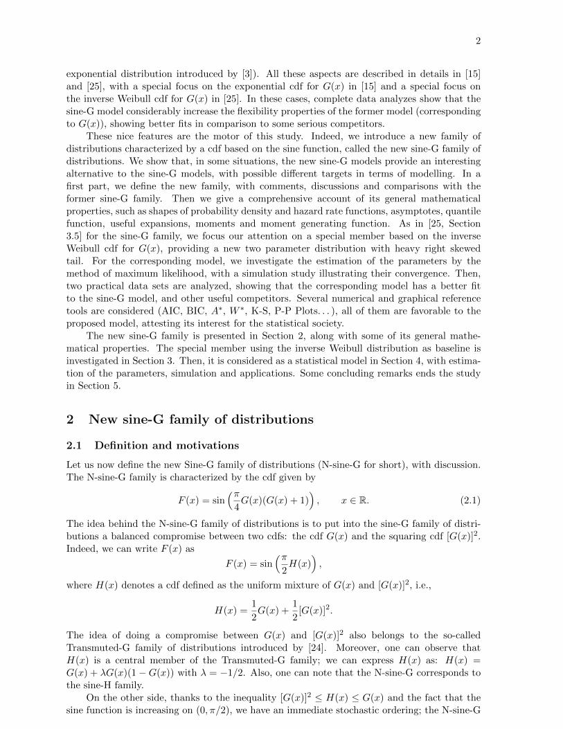
2

exponential distribution introduced by [3]). All these aspects are described in details in [15]and [25], with a special focus on the exponential cdf for G(x) in [15] and a special focus onthe inverse Weibull cdf for G(x) in [25]. In these cases, complete data analyzes show that thesine-G model considerably increase the flexibility properties of the former model (correspondingto G(x)), showing better fits in comparison to some serious competitors.

These nice features are the motor of this study. Indeed, we introduce a new family ofdistributions characterized by a cdf based on the sine function, called the new sine-G family ofdistributions. We show that, in some situations, the new sine-G models provide an interestingalternative to the sine-G models, with possible different targets in terms of modelling. In afirst part, we define the new family, with comments, discussions and comparisons with theformer sine-G family. Then we give a comprehensive account of its general mathematicalproperties, such as shapes of probability density and hazard rate functions, asymptotes, quantilefunction, useful expansions, moments and moment generating function. As in [25, Section3.5] for the sine-G family, we focus our attention on a special member based on the inverseWeibull cdf for G(x), providing a new two parameter distribution with heavy right skewedtail. For the corresponding model, we investigate the estimation of the parameters by themethod of maximum likelihood, with a simulation study illustrating their convergence. Then,two practical data sets are analyzed, showing that the corresponding model has a better fitto the sine-G model, and other useful competitors. Several numerical and graphical referencetools are considered (AIC, BIC, A∗, W ∗, K-S, P-P Plots. . . ), all of them are favorable to theproposed model, attesting its interest for the statistical society.

The new sine-G family is presented in Section 2, along with some of its general mathe-matical properties. The special member using the inverse Weibull distribution as baseline isinvestigated in Section 3. Then, it is considered as a statistical model in Section 4, with estima-tion of the parameters, simulation and applications. Some concluding remarks ends the studyin Section 5.

2 New sine-G family of distributions

2.1 Definition and motivations

Let us now define the new Sine-G family of distributions (N-sine-G for short), with discussion.The N-sine-G family is characterized by the cdf given by

F (x) = sin(π

4G(x)(G(x) + 1)

), x ∈ R. (2.1)

The idea behind the N-sine-G family of distributions is to put into the sine-G family of distri-butions a balanced compromise between two cdfs: the cdf G(x) and the squaring cdf [G(x)]2.Indeed, we can write F (x) as

F (x) = sin(π

2H(x)

),

where H(x) denotes a cdf defined as the uniform mixture of G(x) and [G(x)]2, i.e.,

H(x) =1

2G(x) +

1

2[G(x)]2.

The idea of doing a compromise between G(x) and [G(x)]2 also belongs to the so-calledTransmuted-G family of distributions introduced by [24]. Moreover, one can observe thatH(x) is a central member of the Transmuted-G family; we can express H(x) as: H(x) =G(x) + λG(x)(1−G(x)) with λ = −1/2. Also, one can note that the N-sine-G corresponds tothe sine-H family.

On the other side, thanks to the inequality [G(x)]2 ≤ H(x) ≤ G(x) and the fact that thesine function is increasing on (0, π/2), we have an immediate stochastic ordering; the N-sine-G

3

cdf can be bounded by two cdfs: one of the sine-G family and the other of the sine-G2 family,as

sin(π

2[G(x)]2

)≤ F (x) ≤ sin

(π2G(x)

).

In this sense, the N-sine-G family provides a simple alternative to the sine-G family, withdifferent target in terms of modelling. This practical aspect will be developed in Section 4.Also, observe that no new parameter has been added, respecting the prime idea of the sine-Gfamily.

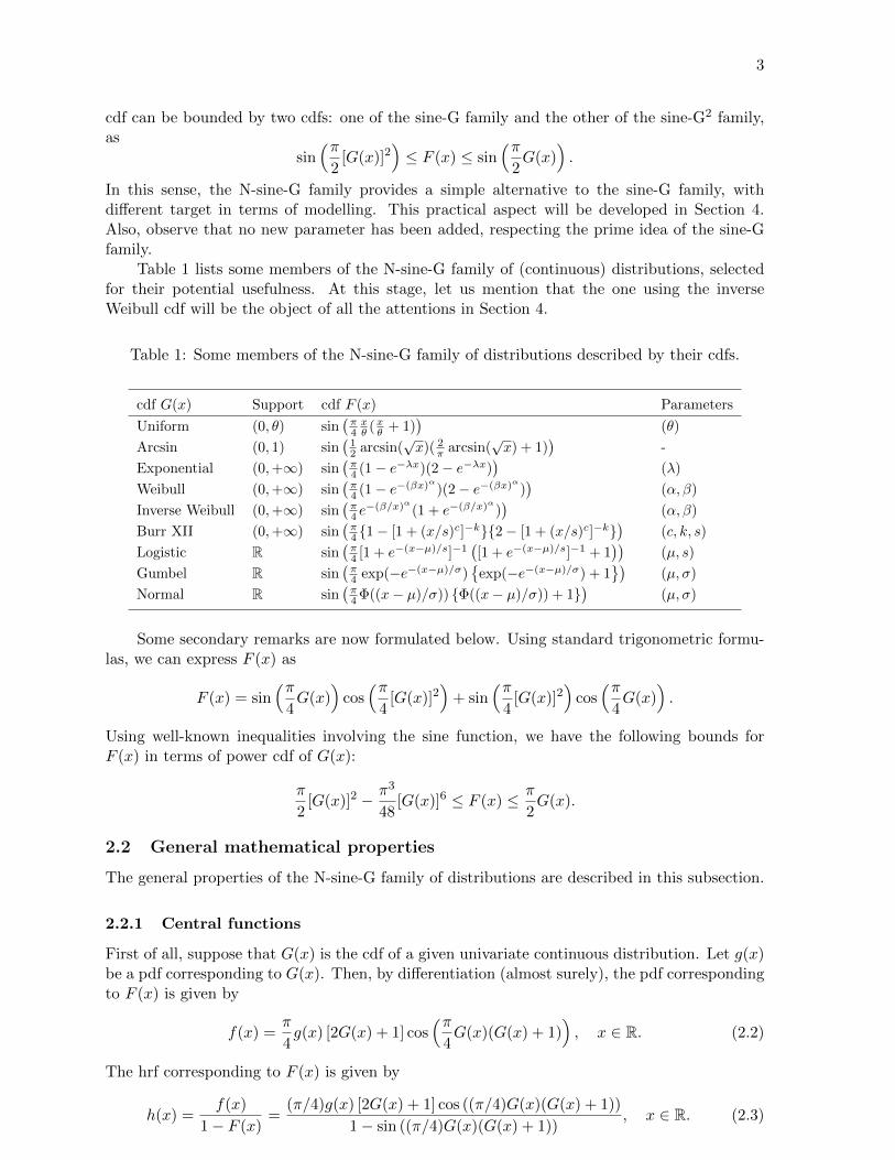
Table 1 lists some members of the N-sine-G family of (continuous) distributions, selectedfor their potential usefulness. At this stage, let us mention that the one using the inverseWeibull cdf will be the object of all the attentions in Section 4.

Table 1: Some members of the N-sine-G family of distributions described by their cdfs.

cdf G(x) Support cdf F (x) Parameters

Uniform (0, θ) sin(π4xθ (xθ + 1)

)(θ)

Arcsin (0, 1) sin(12 arcsin(

√x)( 2

π arcsin(√x) + 1)

)-

Exponential (0,+∞) sin(π4 (1− e−λx)(2− e−λx)

)(λ)

Weibull (0,+∞) sin(π4 (1− e−(βx)α)(2− e−(βx)α)

)(α, β)

Inverse Weibull (0,+∞) sin(π4 e

−(β/x)α(1 + e−(β/x)α))

(α, β)

Burr XII (0,+∞) sin(π4 {1− [1 + (x/s)c]−k}{2− [1 + (x/s)c]−k}

)(c, k, s)

Logistic R sin(π4 [1 + e−(x−µ)/s]−1

([1 + e−(x−µ)/s]−1 + 1

))(µ, s)

Gumbel R sin(π4 exp(−e−(x−µ)/σ)

{exp(−e−(x−µ)/σ) + 1

})(µ, σ)

Normal R sin(π4 Φ((x− µ)/σ)) {Φ((x− µ)/σ)) + 1}

)(µ, σ)

Some secondary remarks are now formulated below. Using standard trigonometric formu-las, we can express F (x) as

F (x) = sin(π

4G(x)

)cos(π

4[G(x)]2

)+ sin

(π4

[G(x)]2)

cos(π

4G(x)

).

Using well-known inequalities involving the sine function, we have the following bounds forF (x) in terms of power cdf of G(x):

π

2[G(x)]2 − π3

48[G(x)]6 ≤ F (x) ≤ π

2G(x).

2.2 General mathematical properties

The general properties of the N-sine-G family of distributions are described in this subsection.

2.2.1 Central functions

First of all, suppose that G(x) is the cdf of a given univariate continuous distribution. Let g(x)be a pdf corresponding to G(x). Then, by differentiation (almost surely), the pdf correspondingto F (x) is given by

f(x) =π

4g(x) [2G(x) + 1] cos

(π4G(x)(G(x) + 1)

), x ∈ R. (2.2)

The hrf corresponding to F (x) is given by

h(x) =f(x)

1− F (x)=

(π/4)g(x) [2G(x) + 1] cos ((π/4)G(x)(G(x) + 1))

1− sin ((π/4)G(x)(G(x) + 1)), x ∈ R. (2.3)

4

Note that, using standard trigonometric formulas, we can express f(x) as

f(x) =π

4g(x) [2G(x) + 1]

[cos(π

4G(x)

)cos(π

4[G(x)]2

)− sin

(π4

[G(x)]2)

sin(π

4G(x)

)].

2.2.2 Critical points and asymptotes

Some features on the variations of the functions F (x), f(x) and h(x) are described below. Thecritical points of f(x) are the solution x0 of the nonlinear equation f ′(x0) = 0, i.e.,

cos(π

4G(x0)(G(x0) + 1)

) [π2G(x0)g

′(x0) +π

4g′(x0) +

π

2[g(x0)]

2]

−[π

2G(x0)g(x0) +

π

4g(x0)

]2sin(π

4G(x0)(G(x0) + 1)

)= 0. (2.4)

The critical points of h(x) are the solution x∗ of the nonlinear equation h′(x∗) = 0, i.e.,

4[2G(x∗) + 1]g′(x∗) cos(π

4G(x∗)(G(x∗) + 1)

)+ [g(x∗)]

2

[4π[G(x∗)]

2 + 4πG(x∗)

+ 8 cos(π

4G(x∗)(G(x∗) + 1)

)+ π

]= 0. (2.5)

We can determine the nature of the critical point by determining the sign of the second derivativeof the function taken at this point.

The asymptotes for F (x), f(x) and h(x) are given below. When G(x)→ 0, using sin(y) ∼ ywhen y → 0, we have

F (x) ∼ π

4G(x), f(x) ∼ π

4g(x), h(x) ∼ π

4g(x).

When G(x)→ 1, using sin(y) = cos(π/2− y) ∼ 1− (π/2− y)2/2 and cos(y) = sin(π/2− y) ∼π/2− y, when y → π/2, we have

F (x) ∼ 1− π2

8

(1− 1

2G(x)(G(x) + 1)

)2

, f(x) ∼ 3π2

8g(x)

(1− 1

2G(x)(G(x) + 1)

)and

h(x) ∼ 3g(x)

1− (1/2)G(x)(G(x) + 1).

2.2.3 Quantile function

Let QG(x) be the quantile function (qf) corresponding to G(x), i.e., satisfying G(QG(y)) = yfor y ∈ (0, 1). Then, the qf corresponding to F (x) is given by

QF (y) = QG

(√4

πarcsin(y) +

1

4− 1

2

), y ∈ (0, 1). (2.6)

In particular, the median given by MedF = QF (0.5) = QG(x∗) with x∗ ≈ 0.4574271.Some important practical applications of QF (y) are the following. Let U be a random

variable following the uniform distribution over (0, 1). Then, the random variable X = QF (U)has the cdf F (x) given by (2.1). For a given G(x), this can be used to simulate different valuesdistributed following the corresponding N-sine-G distribution. Moreover, the quantile densityfunction of X can be obtained by differentiating QF (y) with respect to y.

On the other side, the analysis of the variability of the skewness and kurtosis can beinvestigated based on quantile measures as the Bowley skewness (see [13]) and the Moorskurtosis (see [19]), respectively. The Bowley skewness based on quartiles is given by

B =QF (3/4) +QF (1/4)− 2QF (2/4)

QF (3/4)−QF (1/4).

5

The Moors kurtosis based on octiles is given by

M =QF (3/8)−QF (1/8) +QF (7/8)−QF (5/8)

QF (6/8)−QF (2/8).

2.2.4 Useful expansions

Proposition 2.1 The cdf F (x) given by (2.1) can be expressed as sums of power cdfs, i.e., of

the form [G(x)]θ, where θ is an integer.

Proof. Using the series expansions for the sine function, we have

F (x) = sin(π

4G(x)(G(x) + 1)

)=

+∞∑k=0

(−1)k

(2k + 1)!

(π4

)2k+1[G(x)]2k+1(G(x) + 1)2k+1.

Then, the binomial formula gives

F (x) =+∞∑k=0

2k+1∑`=0

ak,`[G(x)]`+2k+1,

where

ak,` =(−1)k

(2k + 1)!

(π4

)2k+1 (2k + 1)!

`!(2k + 1− `)!. (2.7)

This completes the proof of Proposition 2.1. �

It follows from Proposition 2.1 that, by differentiation under the sums, we can express thepdf as

f(x) =+∞∑k=0

2k+1∑`=0

bk,`[G(x)]`+2kg(x), (2.8)

where bk,` = (`+2k+1)ak,`. Moreover, the properties of the power cdfs of the form [G(x)]θ canbe used to determine transformation involving f(x) as the integrals, and, a fortiori, statisticalproperties on X. The next subsection applies this result to express moments of various kind.

2.2.5 Moments

Let X be a random variable having the cdf F (x). Then the rth moment of X is given byµ′r = E(Xr) =

∫ +∞−∞ xrf(x)dx. Using the series expansions (2.8), assuming that the sum and

integral terms exist, we obtain

µ′r =

+∞∑k=0

2k+1∑`=0

bk,`

∫ +∞

−∞xr[G(x)]`+2kg(x)dx. (2.9)

Note that∫ +∞−∞ xr[G(x)]`+2kg(x)dx =

∫ 10 x

`+2k[QG(x)]rdx. This integral has not necessarily aclose form. We can at least compute numerically by using a standard software (R, Matlab,Mathematica. . . ).

6

From µ′r, we can deduce the mean of X given by E(X) = µ′1, the variance of X given byV(X) = µ′2− (µ′1)

2, the standard deviation of X given by σ(X) =√µ′2 − (µ′1)

2, the , coefficientof variation given by CV = σ(X)/µ′1, the rth central moment of X given by

µr = E[(X − µ′1)r

]=

r∑k=0

r!

k!(r − k)!(−1)k(µ′1)

kµ′r−k,

the coefficient of skewness given by CS = µ3/µ3/22 , the coefficient of kurtosis given by CK =

µ4/µ22, and the rth descending factorial moment of X is given by

µ(r) = E [X(X − 1) . . . (X − r + 1)] =r∑

k=0

sr,kµ′k,

where sr,k denotes the Stirling number of the first kind.The moment generating function of X is given by M(t) = E(etX) with t ≤ 0 (to ensure

its existence, this domain of definition can be refined according to the definition G(x)). Byassuming that the sum and integral terms exist, we obtain

M(t) =+∞∑k=0

2k+1∑`=0

bk,`

∫ +∞

−∞etx[G(x)]`+2kg(x)dx.

Note that∫ +∞−∞ etx[G(x)]`+2kg(x)dx =

∫ 10 x

`+2ketQG(x)dx. Again, we can determine it numeri-cally for a given G(x). As usual, we have the following relation between the rth moments andthe moment generating function: µ′r = M (r)(t) |t=0 for any integer r.

Other probabilistic can be express in a similar manner, as the characteristic function, theconditional moments and the mean deviations. See, for instance, the methodology of [10].

3 The N-sine-IW distribution

3.1 Presentation

We now present a special member of N-sine-G family of distributions with support on (0,+∞)using the cdf G(x) of the inverse Weibull distribution given by G(x) = e−(β/x)

α, α, β, x > 0 (see

[11]). We thus aim to construct a new heavy right skew model for real life data, by increasingthe flexibility of the former inverse Weibull distribution. Hereafter, this special member will becalled the N-sine-IW(α, β) distribution. By using the cdf given by (2.1), the N-sine-IW(α, β)distribution is characterized by the cdf given by

F (x) = sin(π

4e−(β/x)

α(e−(β/x)

α+ 1)

), x > 0. (3.1)

By using (2.2) and (2.3) with g(x) = αβαx−α−1e−(β/x)α, the corresponding pdf is given by

f(x) =π

4αβαx−α−1e−(β/x)

α[2e−(β/x)

α+ 1]

cos(π

4e−(β/x)

α(e−(β/x)

α+ 1)

), x > 0, (3.2)

and the corresponding hrf is given by

h(x) =(π/4)αβαx−α−1e−(β/x)

α [2e−(β/x)

α+ 1]

cos((π/4)e−(β/x)

α(e−(β/x)

α+ 1)

)1− sin

((π/4)e−(β/x)α(e−(β/x)α + 1)

) , x > 0.

The critical points for f(x) and h(x) can be obtained by solving the equations (2.4) and (2.5),respectively. The asymptotes for F (x), f(x) and h(x) are given below. When x→ 0, we have

F (x) ∼ π

4e−(β/x)

α → 0, f(x) ∼ π

4αβαx−α−1e−(β/x)

α → 0

7

andh(x) ∼ π

4αβαx−α−1e−(β/x)

α → 0.

When x→ +∞, we have

F (x) ∼ 1− 9π2

32β2αx−2α → 1, f(x) ∼ 9

π2

16αβ2αx−2α−1 → 0, h(x) ∼ 2αx−1 → 0.

We can remark that f(x) as a polynomial decay when x → +∞. Moreover, when x → +∞,the asymptote of h(x) depends only on the parameter α.

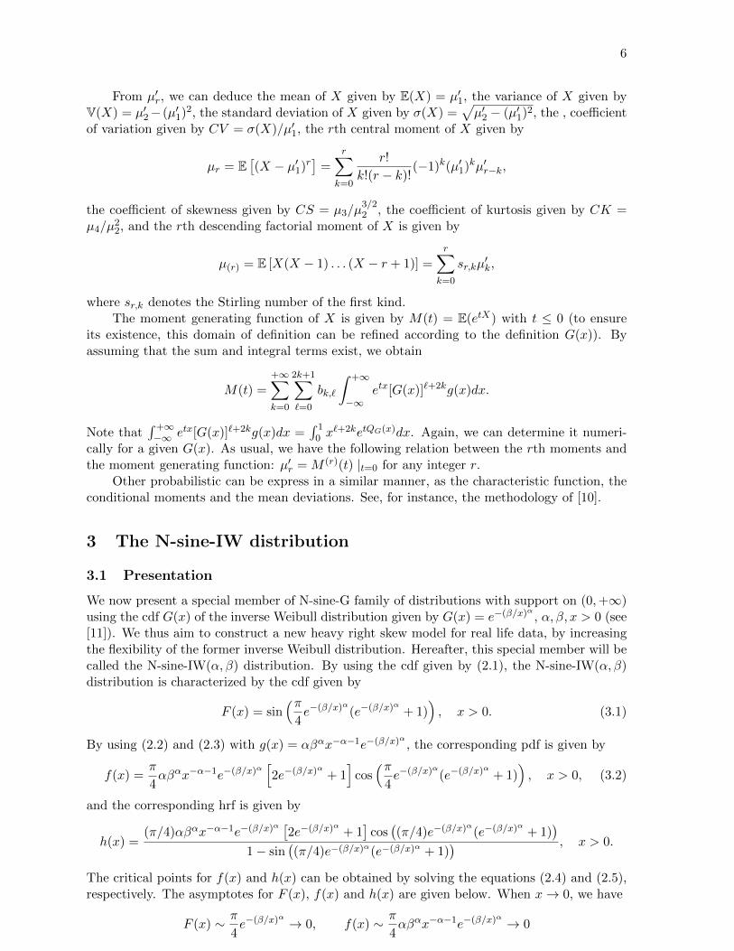
Figure 1 shows the plots for f(x) and h(x) respectively, for selected values for α and β.Various forms of right skew tail curvatures are observed, attesting the ability of the N-sine-IW(α, β) to model a wide variety of life-time data sets having such form of histogram.

0.0 0.5 1.0 1.5 2.0 2.5 3.0

0.0

0.5

1.0

1.5

2.0

2.5

3.0

x

f(x)

α = 0.3 β = 0.4α = 0.9 β = 0.5α = 2.4 β = 0.95α = 10.1 β = 2

0 2 4 6 8 10

02

46

x

h(x)

α = 0.8 β = 0.1α = 0.9 β = 0.5α = 1.8 β = 0.7α = 10.1 β = 2

(a) (b)

Figure 1: (a) Curves for the pdf f(x) (b) Curves for the hrf h(x) for selected values of the

parameters.

3.2 Quantile function

Let us remark that the qf corresponding to G(x) is given by QG(y) = β [− ln(y)]−1/α, y ∈ (0, 1).Then, by virtue of (2.6), the qf of the N-sine-IW(α, β) distribution is given by

QF (y) = β

[− ln

(√4

πarcsin(y) +

1

4− 1

2

)]−1/α, y ∈ (0, 1).

Let U be a random variable following the uniform distribution over (0, 1). Then X = QF (U)follows the N-sine-IW(α, β) distribution. As an immediate consequence, data distributed fol-lowing the N-sine-IW(α, β) distribution can be simulated. The median of the N-sine-IW(α, β)distribution is given by

MedF = QF (0.5) = β

[− ln

(√4

πarcsin(0.5) +

1

4− 1

2

)]−1/α.

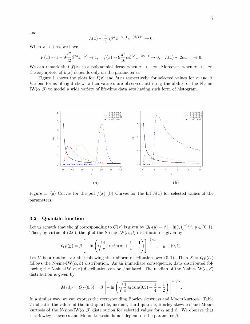
In a similar way, we can express the corresponding Bowley skewness and Moors kurtosis. Table2 indicates the values of the first quartile, median, third quartile, Bowley skewness and Moorskurtosis of the N-sine-IW(α, β) distribution for selected values for α and β. We observe thatthe Bowley skewness and Moors kurtosis do not depend on the parameter β.

8

Table 2: First quartile, median, third quartile, Bowley skewness and Moors kurtosis of the

N-sine-IW(α, β) distribution for the following selected parameters values in order (α, β): (i):

(2.5, 0.3), (ii): (2.5, 1), (iii): (2.5, 2), (iv): (3, 5) and (v): (6, 1).

QF (1/4) MedF QF (3/4) B M

(i) 0.265 0.331 0.422 0.161 1.332

(ii) 0.884 1.103 1.407 0.161 1.332

(iii) 1.767 2.207 2.814 0.161 1.332

(iv) 4.511 5.427 6.645 0.142 1.314

(v) 0.950 1.042 1.153 0.094 1.279

3.3 Moments

Let X be a random variable following the N-sine-IW(α, β) distribution. Then X has a rthmoment if and only if r ∈ (0, 2α). Indeed, there is no problem for x→ 0 and for x→ +∞, wehave

xrf(x) ∼ 9π2

16αβ2αxr−2α−1,

and∫ +∞1 xr−2α−1dx exists as a Riemann integral if and only if r ∈ (0, 2α). For given values for

r, α and β, the integral expression of µ′r can be evaluated numerically. On the other hand, forr ∈ (0, α), the rth moment of X can be obtained by the formula given by (2.9), i.e.,

µ′r =+∞∑k=0

2k+1∑`=0

bk,`

∫ +∞

−∞xr[G(x)]`+2kg(x)dx.

The integral terms can be expressed via gamma functions, as developed below. Let us considerthe gamma function Γ(x) =

∫ +∞0 tx−1e−tdt with x > 0. By the change of variable y = (` +

2k + 1)(β/x)α, we have∫ +∞

−∞xr[G(x)]`+2kg(x)dx = αβα

∫ +∞

0xr−α−1e−(`+2k+1)(β/x)αdx

= βr(`+ 2k + 1)r/α−1Γ(

1− r

α

).

By noticing that (`+ 2k+ 1)r/α−1bk,` = (`+ 2k+ 1)r/αak,`, where ak,` is given by (2.7), we have

µ′r = βrΓ(

1− r

α

) +∞∑k=0

2k+1∑`=0

ak,`(`+ 2k + 1)r/α.

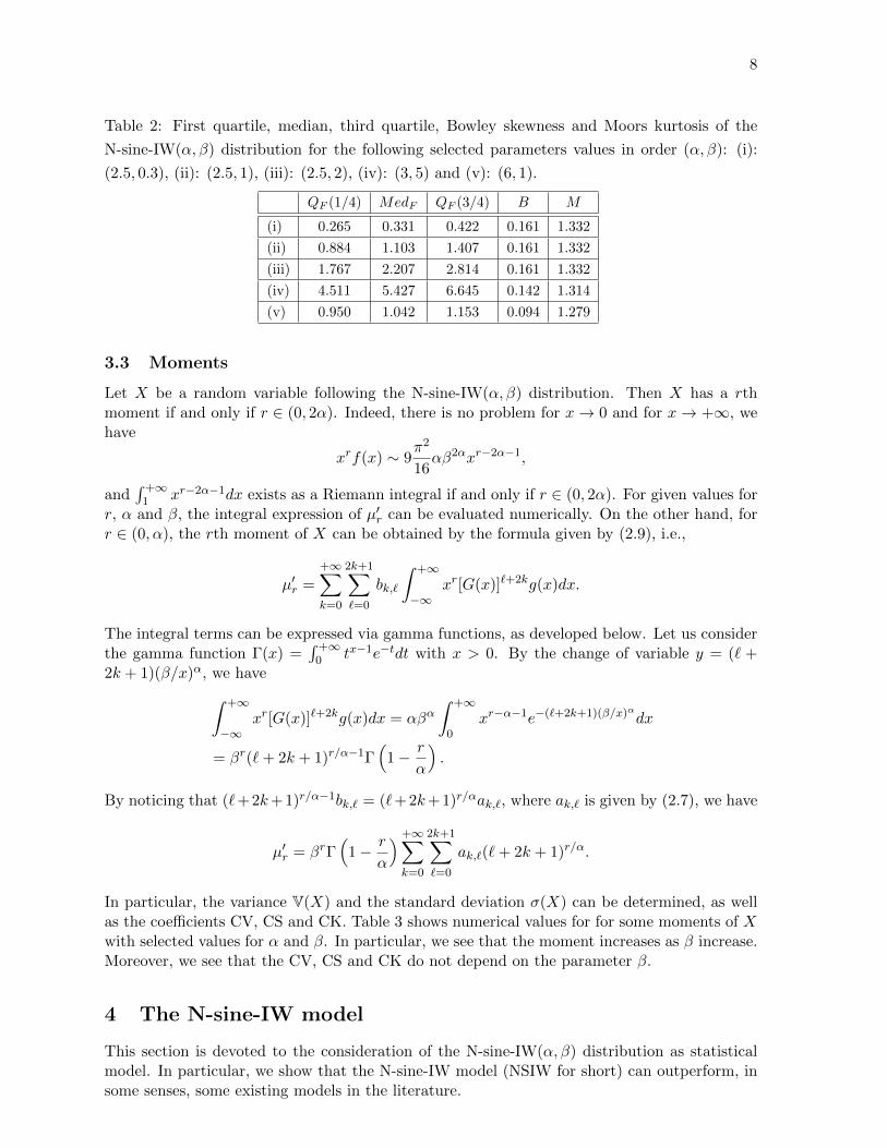
In particular, the variance V(X) and the standard deviation σ(X) can be determined, as wellas the coefficients CV, CS and CK. Table 3 shows numerical values for for some moments of Xwith selected values for α and β. In particular, we see that the moment increases as β increase.Moreover, we see that the CV, CS and CK do not depend on the parameter β.

4 The N-sine-IW model

This section is devoted to the consideration of the N-sine-IW(α, β) distribution as statisticalmodel. In particular, we show that the N-sine-IW model (NSIW for short) can outperform, insome senses, some existing models in the literature.

9

Table 3: Some moments of the N-sine-IW(α, β) distribution for the following selected param-

eters values in order (α, β): (i): (2.5, 0.3), (ii): (2.5, 1), (iii): (2.5, 2), (iv): (3, 5) and (v):

(6, 1).

E(X) E(X2) E(X3) E(X4) V(X) σ(X) CV CS CK

(i) 0.364 0.156 0.084 0.069 0.023 0.153 0.420 2.861 32.967

(ii) 1.213 1.731 3.105 8.496 0.259 0.509 0.420 2.861 32.967

(iii) 2.426 6.923 24.842 135.939 1.036 1.018 0.420 2.861 32.967

(iv) 5.814 37.634 279.681 2543.236 3.828 1.957 0.337 2.183 16.624

(v) 1.065 1.163 1.303 1.505 0.028 0.167 0.156 1.164 6.219

4.1 Maximum likelihood estimation

We propose to estimate the parameter α and β of the NSIW model by the maximum likeli-hood method. Let x1, . . . , xn be a sample of a random variable following the N-sine-IW(α, β)distribution. By using the pdf f(x) given by (3.2), the likelihood function is defined by

L(α, β) =n∏i=1

f(xi)

=(π

4

)nαnβnα

(n∏i=1

xi

)−α−1e−

n∑i=1

(β/xi)α n∏i=1

[2e−(β/xi)

α+ 1] n∏i=1

cos(π

4e−(β/xi)

α(e−(β/xi)

α+ 1)

).

The log-likelihood function is given by

`(α, β) = logL(α, β)

= n log(π

4

)+ n log(α) + nα log(β)− (α+ 1)

n∑i=1

log(xi)−n∑i=1

(β

xi

)α+

n∑i=1

log[2e−(β/xi)

α+ 1]

+n∑i=1

log[cos(π

4e−(β/xi)

α(e−(β/xi)

α+ 1)

)].

The maximum likelihood estimators (MLEs) are solution of the nonlinear equations: ∂`(α, β)/∂α =0 and ∂`(α, β)/∂β = 0, with

∂

∂α`(α, β) = n

(1

α+ log(β)

)−

n∑i=1

log (xi)−n∑i=1

(β

xi

)αlog

(β

xi

)

− 2

n∑i=1

e−(β/xi)α

(β/xi)α log (β/xi)

2e−(β/xi)α

+ 1

+π

4

n∑i=1

e−(β/xi)α[2e−(β/xi)

α+ 1]( β

xi

)αlog

(β

xi

)tan

(π4e−(β/xi)

α(e−(β/xi)

α+ 1)

)and

∂

∂β`(α, β) =

αn

β− α

n∑i=1

1

xi

(β

xi

)α−1− 2α

n∑i=1

e−(β/xi)α

(β/xi)α−1

xi(2e−(β/xi)

α+ 1)

+π

4

α

β

n∑i=1

e−(β/xi)α[2e−(β/xi)

α+ 1]( β

xi

)αtan

(π4e−(β/xi)

α(e−(β/xi)

α+ 1)

).

10

These equation can not be solved analytically. Numerical solutions exist by the use ofiterative methods such as Newton-Raphson type algorithms. Under standard regularity con-ditions, it is well establish that the MLEs are asymptotically unbiased and normal. This lastproperty allows us to construct approximate confidence intervals (CI) and Likelihood ratio testsfor the parameters. In particular, the CIS of α and β are of the form [L.bound, U.bound], whereL.bound denotes the lower bound of the interval and U.bound the upper bound, both dependingon the fixed level of the CI and the components of the estimated Fisher information matrix.See, for instance, [18].

4.2 Simulations

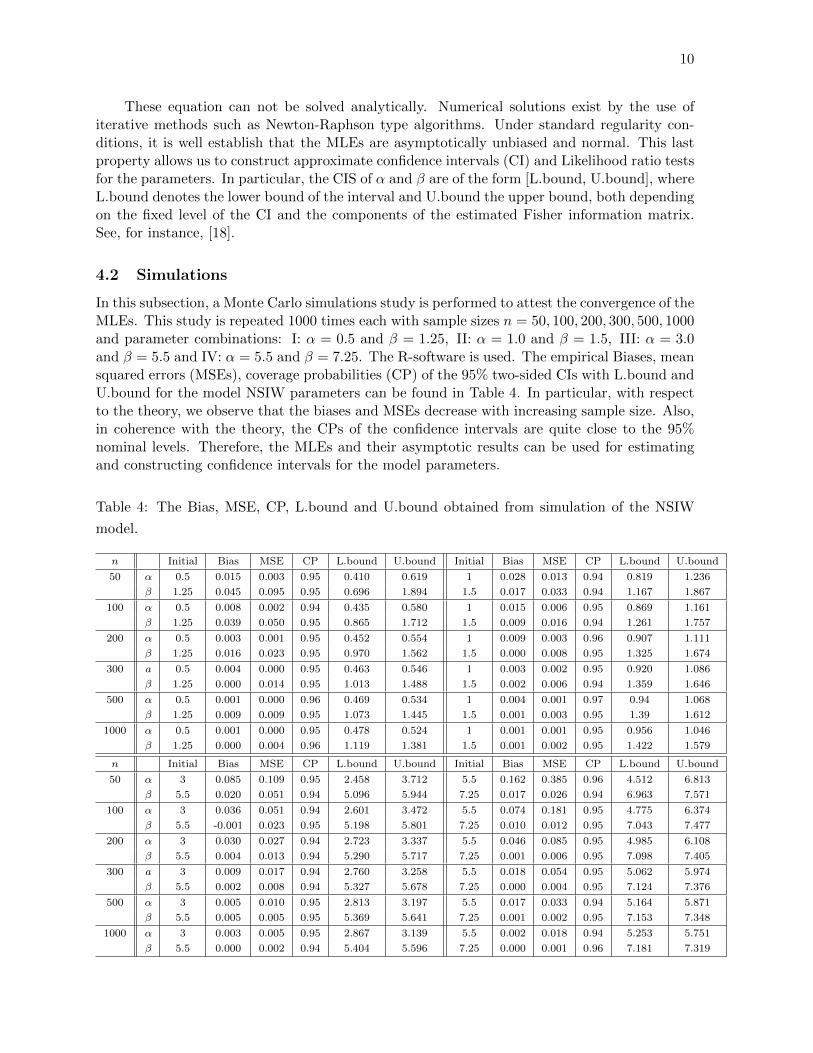
In this subsection, a Monte Carlo simulations study is performed to attest the convergence of theMLEs. This study is repeated 1000 times each with sample sizes n = 50, 100, 200, 300, 500, 1000and parameter combinations: I: α = 0.5 and β = 1.25, II: α = 1.0 and β = 1.5, III: α = 3.0and β = 5.5 and IV: α = 5.5 and β = 7.25. The R-software is used. The empirical Biases, meansquared errors (MSEs), coverage probabilities (CP) of the 95% two-sided CIs with L.bound andU.bound for the model NSIW parameters can be found in Table 4. In particular, with respectto the theory, we observe that the biases and MSEs decrease with increasing sample size. Also,in coherence with the theory, the CPs of the confidence intervals are quite close to the 95%nominal levels. Therefore, the MLEs and their asymptotic results can be used for estimatingand constructing confidence intervals for the model parameters.

Table 4: The Bias, MSE, CP, L.bound and U.bound obtained from simulation of the NSIW

model.

n Initial Bias MSE CP L.bound U.bound Initial Bias MSE CP L.bound U.bound

50 α 0.5 0.015 0.003 0.95 0.410 0.619 1 0.028 0.013 0.94 0.819 1.236

β 1.25 0.045 0.095 0.95 0.696 1.894 1.5 0.017 0.033 0.94 1.167 1.867

100 α 0.5 0.008 0.002 0.94 0.435 0.580 1 0.015 0.006 0.95 0.869 1.161

β 1.25 0.039 0.050 0.95 0.865 1.712 1.5 0.009 0.016 0.94 1.261 1.757

200 α 0.5 0.003 0.001 0.95 0.452 0.554 1 0.009 0.003 0.96 0.907 1.111

β 1.25 0.016 0.023 0.95 0.970 1.562 1.5 0.000 0.008 0.95 1.325 1.674

300 a 0.5 0.004 0.000 0.95 0.463 0.546 1 0.003 0.002 0.95 0.920 1.086

β 1.25 0.000 0.014 0.95 1.013 1.488 1.5 0.002 0.006 0.94 1.359 1.646

500 α 0.5 0.001 0.000 0.96 0.469 0.534 1 0.004 0.001 0.97 0.94 1.068

β 1.25 0.009 0.009 0.95 1.073 1.445 1.5 0.001 0.003 0.95 1.39 1.612

1000 α 0.5 0.001 0.000 0.95 0.478 0.524 1 0.001 0.001 0.95 0.956 1.046

β 1.25 0.000 0.004 0.96 1.119 1.381 1.5 0.001 0.002 0.95 1.422 1.579

n Initial Bias MSE CP L.bound U.bound Initial Bias MSE CP L.bound U.bound

50 α 3 0.085 0.109 0.95 2.458 3.712 5.5 0.162 0.385 0.96 4.512 6.813

β 5.5 0.020 0.051 0.94 5.096 5.944 7.25 0.017 0.026 0.94 6.963 7.571

100 α 3 0.036 0.051 0.94 2.601 3.472 5.5 0.074 0.181 0.95 4.775 6.374

β 5.5 -0.001 0.023 0.95 5.198 5.801 7.25 0.010 0.012 0.95 7.043 7.477

200 α 3 0.030 0.027 0.94 2.723 3.337 5.5 0.046 0.085 0.95 4.985 6.108

β 5.5 0.004 0.013 0.94 5.290 5.717 7.25 0.001 0.006 0.95 7.098 7.405

300 a 3 0.009 0.017 0.94 2.760 3.258 5.5 0.018 0.054 0.95 5.062 5.974

β 5.5 0.002 0.008 0.94 5.327 5.678 7.25 0.000 0.004 0.95 7.124 7.376

500 α 3 0.005 0.010 0.95 2.813 3.197 5.5 0.017 0.033 0.94 5.164 5.871

β 5.5 0.005 0.005 0.95 5.369 5.641 7.25 0.001 0.002 0.95 7.153 7.348

1000 α 3 0.003 0.005 0.95 2.867 3.139 5.5 0.002 0.018 0.94 5.253 5.751

β 5.5 0.000 0.002 0.94 5.404 5.596 7.25 0.000 0.001 0.96 7.181 7.319

11

4.3 Applications

In this section, we presented the analysis of two practical data sets via different models, with afocus on the NSIW model.

4.3.1 Data sets

Data set 1. The first data set contains 72 survival times in days of guinea pigs, voluntarycontaminated with different doses of tubercle bacilli. The source of this data set is [4]. The 72values of this data set are listed below: 12, 15, 22, 24, 24, 32, 32, 33, 34, 38, 38, 43, 44, 48 , 52,53, 54, 54, 55, 56, 57, 58, 58, 59, 60, 60, 60, 60, 61, 62, 63, 65, 65, 67, 68, 70, 70, 72, 73, 75, 76,76, 81, 83, 84, 85, 87, 91, 95, 96, 98, 99, 109, 110, 121, 127, 129, 131, 143, 146, 146, 175, 175,211, 233, 258, 258, 263, 297, 341, 341, 376.Figures 2 (a) presents the histogram of data set 1, showing a heavy right tail, also indicated bythe TTT plot in Figure 2 (b). The boxplot of data set 1 can be seen in Figure 3 (a) and theQ-Q plot in Figure 3 (b). From these graphics, we clearly see that the normal distribution ismisappropriated, motivating the use of a model with heavy right tail, as the NSIW model forinstance.

Histogram of x

x

Den

sity

0 100 200 300 400

0.00

00.

002

0.00

40.

006

0.00

80.

010

0.0 0.2 0.4 0.6 0.8 1.0

0.0

0.2

0.4

0.6

0.8

1.0

i/n

T(i/

n)

(a) (b)

Figure 2: (a) Histogram (b) TTT plot for data set 1.

12

010

020

030

0

−2 −1 0 1 2

010

020

030

0

Normal Q−Q Plot

Theoretical Quantiles

Sam

ple

Qua

ntile

s

(a) (b)

Figure 3: (a) Boxplot (b) Normal Q-Q plot for data set 1.

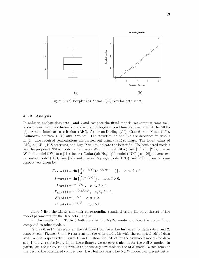
Data set 2. The second data set contains 23 numbers of million of revolutions before failureof a ball bearing. The source of this data sets is [16]. The 23 values of this data set are listedbelow: 17.88, 28.92, 33.00, 41.52, 42.12, 45.60, 48.80, 51.84, 51.96, 54.12, 55.56, 67.80, 68.44,68.64, 68.88, 84.12, 93.12, 98.64, 105.12, 105.84, 127.92, 128.04, 173.40The histogram of data set 2 is given in Figures 4 (a). We clearly see a heavy right tail, confirmedby the TTT plot in Figure 4 (b). The boxplot of data set 2 is presented in Figure 5 (a) and theQ-Q plot in Figure 5 (b). The normal model is clearly not the best for this data set; a modelwith heavy right tail is required, motivating the use of the NSIW model.

Histogram of x

x

Den

sity

0 50 100 150

0.00

00.

005

0.01

00.

015

0.0 0.2 0.4 0.6 0.8 1.0

0.0

0.2

0.4

0.6

0.8

1.0

i/n

T(i/

n)

(a) (b)

Figure 4: (a) Histogram (b) TTT plot for data set 2.

13

50

10

01

50

−2 −1 0 1 2

5010

015

0

Normal Q−Q Plot

Theoretical Quantiles

Sam

ple

Qua

ntile

s

(a) (b)

Figure 5: (a) Boxplot (b) Normal Q-Q plot for data set 2.

4.3.2 Analysis

In order to analyze data sets 1 and 2 and compare the fitted models, we compute some well-known measures of goodness-of-fit statistics: the log-likelihood function evaluated at the MLEs(ˆ), Akaike information criterion (AIC), Anderson-Darling (A∗), Cramer–von Mises (W ∗),Kolmogrov-Smirnov (K-S) and P-values. The statistics A∗ and W ∗ are described in detailsin [6]. The required computations are carried out using the R-software. The lower values ofAIC, A∗, W ∗ , K-S statistics, and high P-values indicate the better fit. The considered modelsare the proposed NSIW model, sine inverse Weibull model (SIW) (see [15] and [25]), inverseWeibull model (IW) (see [11]), inverse Nadarajah-Haghighi model (INH) (see [26]), inverse ex-ponential model (IED) (see [12]) and inverse Rayleigh model(IRD) (see [27]). Their cdfs arerespectively given by

FNSIW (x) = sin(π

4e−(β/x)

α(e−(β/x)

α+ 1)

), x, α, β > 0,

FSIW (x) = sin(π

2e−(β/x)

α), x, α, β > 0,

FIW (x) = e−(β/x)α, x, α, β > 0,

FINH(x) = e1−(1+β/x)α, x, α, β > 0,

FIED(x) = e−α/x, x, α > 0,

FIRD(x) = e−α/x2, x, α > 0.

Table 5 lists the MLEs and their corresponding standard errors (in parentheses) of themodel parameters for the data sets 1 and 2.

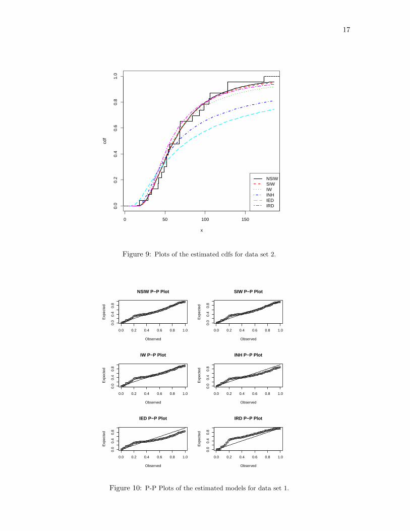
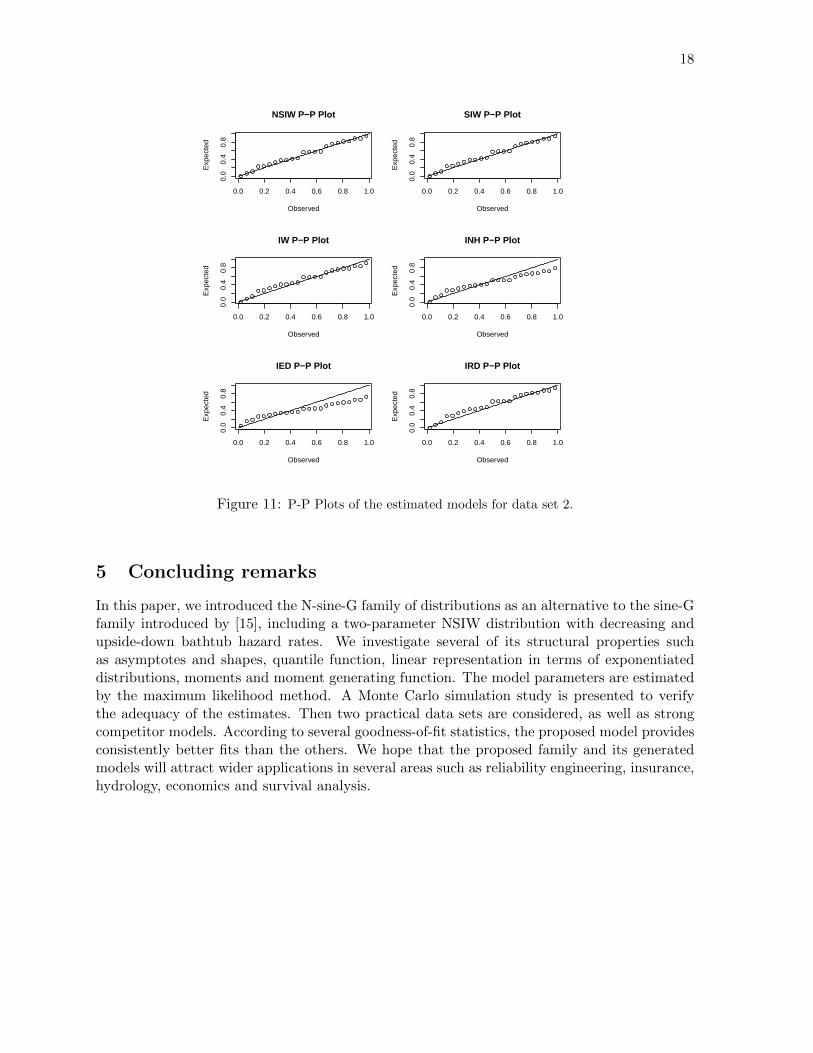
All the results from Table 6 indicate that the NSIW model provides the better fit ascompared to other models.

Figures 6 and 7 represent all the estimated pdfs over the histogram of data sets 1 and 2,respectively. Figures 8 and 9 represent all the estimated cdfs with the empirical cdf of datasets 1 and 2, respectively. Figures 10 and 11 show the P-Plot for the estimated models for datasets 1 and 2, respectively. In all these figures, we observe a nice fit for the NSIW model. Inparticular, the NSIW model reveals to be visually favorable to the SIW model, which remainsthe best of the considered competitors. Last but not least, the NSIW model can present better

14

Table 5: MLEs and their standard errors (in parentheses) for the data sets 1 and 2.

Distribution α β

Data set 1

NSIW 1.187246 59.277943(0.09749533) (4.89936841)

SIW 1.087296 78.679016(0.09010003) (7.12214888)

IW 1.415099 54.154478(0.1172978) (4.7819604)

INH 1.837227 25.777213(0.6195688) (11.9194201)

IED 60.09902 -(7.082733) -

IRD 2124.003 -(250.2112) -

Data set 2

NSIW 1.555214 52.354276(0.221727) (5.828250)

SIW 1.418507 64.874725(0.2050217) (7.9449506)

IW 1.834041 48.612750(0.2691721) (5.8731302)

INH 12.265650 2.913329(46.28737) (11.59465)

IED 54.98987 -(11.46618) -

IRD 2235.817 -(466.2137) -

goodness-of-fits to more sophisticated model, with three parameters or more. For instance, thisis the case for the three parameter gamma inverse Weibull (GIW) model introduced by [21]satisfying AIC = 786.5 and BIC = 793.3 for data set 1 (see [21, Table 1]), and AIC = 232.5and BIC = 235.9 for data set 2 (see [21, Table 2]).

15

Table 6: The statistics ˆ, AIC, BIC, A∗, W ∗, K-S and P-value for the data sets 1 and 2.

Distribution ˆ AIC BIC A∗ W ∗ K-S P-value

Data set 1

NSIW 391.114 786.228 790.7813 0.7421414 0.128227 0.12022 0.2491SIW 391.8296 787.6592 792.2125 0.815797 0.1390462 0.12695 0.1962IW 395.6491 795.4722 799.8516 1.283477 0.2148432 0.15231 0.07082INH 400.4679 804.9357 809.4891 1.427511 0.2398301 0.14121 0.1132IED 402.6718 807.3437 809.6203 0.9225515 0.1561167 0.18466 0.01474IRD 406.7674 815.5347 817.8114 1.994931 0.3371843 0.26145 0.0001062

Data set 2

NSIW 113.9501 231.9001 234.1711 0.2910172 0.03847493 0.09927 0.9604SIW 114.3037 232.6073 234.8783 0.340215 0.04477491 0.10618 0.9335IW 115.7833 235.5666 237.8376 0.5546877 0.07517144 0.13261 0.7654INH 119.027 242.054 244.325 0.76066 0.1063972 0.22877 0.1536IED 121.7296 245.4592 246.5947 0.3238192 0.04286789 0.30567 0.02099IRD 115.967 233.934 235.0695 0.6101612 0.0835341 0.14293 0.6831

x

Den

sity

0 100 200 300

0.00

00.

005

0.01

00.

015

NSIWSIWIWINHIEDIRD

Figure 6: Plots of the estimated pdfs for data set 1.

16

x

Den

sity

0 50 100 150

0.00

00.

005

0.01

00.

015

0.02

0

NSIWSIWIWINHIEDIRD

Figure 7: Plots of the estimated pdfs for data set 2.

0 100 200 300 400

0.0

0.2

0.4

0.6

0.8

1.0

x

cdf

NSIWSIWIWINHIEDIRD

Figure 8: Plots of the estimated cdfs for data set 1.

17

0 50 100 150

0.0

0.2

0.4

0.6

0.8

1.0

x

cdf

NSIWSIWIWINHIEDIRD

Figure 9: Plots of the estimated cdfs for data set 2.

0.0 0.2 0.4 0.6 0.8 1.0

0.0

0.4

0.8

NSIW P−P Plot

Observed

Exp

ecte

d

0.0 0.2 0.4 0.6 0.8 1.0

0.0

0.4

0.8

SIW P−P Plot

Observed

Exp

ecte

d

0.0 0.2 0.4 0.6 0.8 1.0

0.0

0.4

0.8

IW P−P Plot

Observed

Exp

ecte

d

0.0 0.2 0.4 0.6 0.8 1.0

0.0

0.4

0.8

INH P−P Plot

Observed

Exp

ecte

d

0.0 0.2 0.4 0.6 0.8 1.0

0.0

0.4

0.8

IED P−P Plot

Observed

Exp

ecte

d

0.0 0.2 0.4 0.6 0.8 1.0

0.0

0.4

0.8

IRD P−P Plot

Observed

Exp

ecte

d

Figure 10: P-P Plots of the estimated models for data set 1.

18

0.0 0.2 0.4 0.6 0.8 1.0

0.0

0.4

0.8

NSIW P−P Plot

ObservedE

xpec

ted

0.0 0.2 0.4 0.6 0.8 1.0

0.0

0.4

0.8

SIW P−P Plot

Observed

Exp

ecte

d

0.0 0.2 0.4 0.6 0.8 1.0

0.0

0.4

0.8

IW P−P Plot

Observed

Exp

ecte

d

0.0 0.2 0.4 0.6 0.8 1.0

0.0

0.4

0.8

INH P−P Plot

Observed

Exp

ecte

d

0.0 0.2 0.4 0.6 0.8 1.0

0.0

0.4

0.8

IED P−P Plot

Observed

Exp

ecte

d

0.0 0.2 0.4 0.6 0.8 1.0

0.0

0.4

0.8

IRD P−P Plot

Observed

Exp

ecte

d

Figure 11: P-P Plots of the estimated models for data set 2.

5 Concluding remarks

In this paper, we introduced the N-sine-G family of distributions as an alternative to the sine-Gfamily introduced by [15], including a two-parameter NSIW distribution with decreasing andupside-down bathtub hazard rates. We investigate several of its structural properties suchas asymptotes and shapes, quantile function, linear representation in terms of exponentiateddistributions, moments and moment generating function. The model parameters are estimatedby the maximum likelihood method. A Monte Carlo simulation study is presented to verifythe adequacy of the estimates. Then two practical data sets are considered, as well as strongcompetitor models. According to several goodness-of-fit statistics, the proposed model providesconsistently better fits than the others. We hope that the proposed family and its generatedmodels will attract wider applications in several areas such as reliability engineering, insurance,hydrology, economics and survival analysis.

19

References

[1] Al-Faris, R.Q. and Khan, S. (2008). Sine Square Distribution: A New Statistical ModelBased on the Sine Function, Journal of Applied Probability and Statistics, 3, 1, 163-173.

[2] Alzaatreh, A., Lee, C. and Famoye, F. (2013). A new method for generating families ofcontinuous distributions. Metron, 71, 63-79.

[3] Bakouch, H.S., Chesneau, C. and Leao, J. (2018). A new lifetime model with a periodichazard rate and an application, Journal of Statistical Computation and Simulation, 88, 11,2048-2065.

[4] Bjerkedal, T. (1960). Acquisition of resistance in guinea pigs infected with different dosesof virulent tubercle bacilli. Amer J Hygiene, 72, 130-148.

[5] Bourguignon, M., Silva, R.B. and Cordeiro, G.M. (2014). The Weibull-G family of proba-bility distributions, Journal of Data Science, 12, 1253-1268.

[6] Chen, G. and Balakrishnan, N. (1995). A general purpose approximate goodness-of-fit test,Journal of Quality Technology, 27, 154-161.

[7] Eugene, N., Lee, C. and Famoye, F. (2002). Beta-normal distribution and its applications,Communications in Statistics - Theory and Methods, 31, 4, 497-512.

[8] Gilbert, G.K. (1895). The moon’s face; a study of the origin of its features, Bulletin of thePhilosophical Society of Washington, Washington, 12, 241-292.

[9] Gupta, R.C., Gupta, P.I. and Gupta, R.D. (1998). Modeling failure time data by Lehmannalternatives, Communications in statistics-Theory and Methods, 27, 887-904.

[10] Hosseini, B., Afshari, M. and Alizadeh, M. (2018). The Generalized Odd Gamma-G Familyof Distributions: Properties and Applications, Austrian Journal of Statistics, 47, 69-89.

[11] Keller, A.Z. and Kamath, A.R. (1982a). Alternative reliability models for mechanical sys-tems, Third International Conference on Reliability and Maintainability, Toulouse, France,411-415.

[12] Keller, A.Z. and Kamath, A.R. (1982b). Reliability analysis of CNC machine tools, Relia-bility Engineering, 3, 449-473.

[13] Kenney, J.F. and Keeping, E.S. (1962). Mathematics of Statistics, 3 edn, Chapman andHall Ltd, New Jersey.

[14] Kent, J.T. and Tyler, D.E. (1988). Maximum likelihood estimation for the wrapped Cauchydistribution, J. Appl. Statist., 15, 247-254.

[15] Kumar, D., Singh, U. and Singh, S. K. (2015). A New Distribution Using Sine Function-Its Application to Bladder Cancer Patients Data, J. Stat. Appl. Pro., 4, 3, 417-427.

[16] Lawless, J. (1982). Statistical Models and Methods for Lifetime Data, John Wiley andSons, New York.

[17] Marshall, A.N. and Olkin, I. (1997). A new method for adding a parameter to a family ofdistributions with applications to the exponential and Weibull families, Biometrica, 84, 3,641-652.

[18] Millar, R.B. (2011). Maximum likelihood estimation and inference: with examples in R,SAS, and ADMB. Statistics in practice, Wiley, Chichester, West Sussex.

20

[19] Moors, J.J. (1988). A quantile alternative for kurtosis, Journal of the Royal StatisticalSociety: Series D, 37, 25-32.

[20] Nadarajah, S. and Kotz, S. (2006). Beta Trigonometric Distribution, Portuguese EconomicJournal, 5, 3, 207-224.

[21] Pararai, M., Warahena-Liyanage, G. and Oluyede, B.O. (2014). A New Class of General-ized Inverse Weibull Distribution with Applications, Journal of Applied Mathematics andBioinformatics, 4, 17-35.

[22] Raab, D.H. and Green, E.H. (1961). A cosine approximation to the normal distribution,Psychometrika, 26, 4, 447-450.

[23] Ristic, M.M. and Balakrishnan, N. (2012). The gamma-exponentiated exponential distri-bution, Journal of Statistical Computation and Simulation, 82, 8, 1191-1206.

[24] Shaw, W.T. and Buckley, I.R.C. (2009). The alchemy of probability distributions: beyondGram-Charlier expansions, and a skew-kurtotic-normal distribution from a rank transmu-tation map, arXiv preprint arXiv:0901.0434.

[25] Souza, L. (2015). New trigonometric classes of probabilistic distributions, Thesis, Univer-sidade Federal Rural de Pernambuco.

[26] Tahir, M.H., Cordeiro, G.M., Ali, S., Dey, S. and Manzoor, A. (2018). The invertedNadarajah- Haghighi distribution: estimation methods and applications. Journal of Sta-tistical Computation and Simulation, 88, 14, 2775-2798.

[27] Voda, V.G. (1972). On the inverse Rayleigh random variable, Rep Stat Appl Res., 19,13-21.

[28] Zografos, K. and Balakrishnan, N. (2009). On the families of beta-and gamma-generatedgeneralized distribution and associated inference, Statistical Methodology, 6, 4, 344-362.