A new paradigm: the linear isotropic Cosserat model with

conformally invariant curvature energy.

Patrizio Neff ∗and Jena Jeong †

September 7, 2008

Abstract

This is an essay on a linear Cosserat model with weakest possible constitutive assump-tions on the curvature energy still providing for existence, uniqueness and stability. Theassumed curvature energy is the conformally invariant expression µL2

c ‖dev sym∇ axlA‖2,where axlA is the axial vector of the skewsymmetric microrotation A ∈ so(3), dev isthe orthogonal projection on the Lie-algebra sl(3) of trace free matrices and sym is theorthogonal projection onto symmetric matrices. It is observed that unphysical singularstiffening for small samples is avoided in torsion and bending while size effects are stillpresent. The number of Cosserat parameters is reduced from six to four: in additionto the (size-independent) classical linear elastic Lame moduli µ and λ only one Cosseratcoupling constant µc > 0 and one length scale parameter Lc > 0 need to be determined.We investigate those deformations not leading to moment stresses for different curvatureassumptions and we exhibit a novel invariance principle of linear, isotropic Cauchy elas-ticity which is extended to the Cosserat and couple-stress (Koiter-Mindlin) model withconformal curvature.

Key words: polar-materials, microstructure, conformal transformations,structured continua, solid mechanics, variational methods.

AMS 2000 subject classification: 74A35, 74A30, 74C05, 74C10

in preparation for ZAMM

Contents

1 Introduction 2

2 The linear elastic isotropic Cosserat model revisited 42.1 The linear elastic Cosserat model in variational form . . . . . . . . . . . . . . . . 42.2 Non-negativity of the energy . . . . . . . . . . . . . . . . . . . . . . . . . . . . . 52.3 Bounded stiffness for small samples . . . . . . . . . . . . . . . . . . . . . . . . . . 52.4 The linear elastic Cosserat balance equations: strong form . . . . . . . . . . . . . 62.5 The investigated cases . . . . . . . . . . . . . . . . . . . . . . . . . . . . . . . . . 62.6 Scaling and geometry of microstructure . . . . . . . . . . . . . . . . . . . . . . . 6

3 Nullspace of the curvature energy 83.1 The pointwise positive nullspace . . . . . . . . . . . . . . . . . . . . . . . . . . . 83.2 The nullspace for dev alone . . . . . . . . . . . . . . . . . . . . . . . . . . . . . . 83.3 The symmetric nullspace . . . . . . . . . . . . . . . . . . . . . . . . . . . . . . . . 93.4 The conformal nullspace . . . . . . . . . . . . . . . . . . . . . . . . . . . . . . . . 93.5 3D-ICT and boundary conditions . . . . . . . . . . . . . . . . . . . . . . . . . . . 103.6 The geometry of the nullspaces: visualization . . . . . . . . . . . . . . . . . . . . 11∗Corresponding author: Patrizio Neff, AG6, Fachbereich Mathematik, Technische Universitat Darmstadt,

Schlossgartenstrasse 7, 64289 Darmstadt, Germany, email: neff@mathematik.tu-darmstadt.de, Tel.: +49-6151-16-3495†Jena Jeong, Ecole Speciale des Travaux Publics du Batiment et de l’Industrie (ESTP), 28 avenue du President

Wilson, 94234 Cachan Cedex, France, email: jeong@profs.estp.fr

1

4 Nullspaces for the indeterminate couple stress problem 124.1 The indeterminate couple stress model . . . . . . . . . . . . . . . . . . . . . . . . 124.2 Curvature free displacement for pointwise positive curvature . . . . . . . . . . . . 134.3 Curvature free displacement for dev-curvature . . . . . . . . . . . . . . . . . . . . 134.4 Curvature free displacement for symmetric curvature . . . . . . . . . . . . . . . . 144.5 Curvature free displacement for conformal curvature . . . . . . . . . . . . . . . . 154.6 Curl-operator and infinitesimal conformal functions . . . . . . . . . . . . . . . . . 15

5 Conformal invariance for zero bulk modulus 155.1 Conformal invariance in Cauchy elasticity . . . . . . . . . . . . . . . . . . . . . . 155.2 Conformal invariance in Cosserat elasticity . . . . . . . . . . . . . . . . . . . . . 165.3 Conformal invariance in indeterminate couple stress theory . . . . . . . . . . . . 165.4 Universal potential solutions for variable bulk modulus . . . . . . . . . . . . . . . 17

6 Conclusion and open problems 17

7 Appendix 207.1 Infinitesimal conformal mappings (ICT) at a glance . . . . . . . . . . . . . . . . . 207.2 Conformal transformations . . . . . . . . . . . . . . . . . . . . . . . . . . . . . . 207.3 Finite special conformal transformations (FSCT) . . . . . . . . . . . . . . . . . . 20

1 Introduction

We investigate some of the salient novel features of a linear elastic Cosserat model with con-formally invariant curvature energy. This work extends and precises previous work of the firstauthor [22].

General continuum models involving independent rotations have been introduced bythe Cosserat brothers [5] at the beginning of the last century. Their originally nonlinear,geometrically exact development has been largely forgotten for decades only to be rediscoveredin a restricted linearized setting in the early sixties. Since then, the original Cosserat concepthas been generalized in various directions, notably by Eringen and his coworkers who extendedthe Cosserat concept to include also microinertia effects and to rename it subsequently intomicropolar theory. For an overview1 of these so called microcontinuum theories we referto [6, 4, 30]. The Cosserat model includes in a natural way size effects, i.e., small samplesbehave comparatively stiffer than large samples. In classical, size-independent models thiswould lead to an apparent increase of elastic moduli for smaller samples of the same material.

The micropolar theory is perhaps best viewed as a generalized continuum theory in whichmicrostructure details are averaged out by a ”characteristic internal length scale” Lc [2, 7].This last parameter can be considered as the size of a representative volume element (RVE)in heterogeneous media and it is frequently used to model damage and fracture phenomenonin concrete [31]. A dislocated single crystal [24] is another example of a Cosserat continuumfor which lattice curvature is due to geometrically necessary dislocations [29]. Extensions toplasticity have been considered in [26, 25, 10, 32].

The mathematical analysis establishing well-posedness for the infinitesimal strain, Cosseratelastic solid is presented e.g. in [11] and extended in [12] for so called linear microstretch models.This analysis has always been based on the uniform positivity of the free quadratic energyof the Cosserat solid. The first author has extended the existence results for both the Cosseratmodel and the more general micromorphic models to the geometrically exact, finite-strain case,see e.g. [27, 23]. More on the mathematical analysis for the nonlinear case can be found in[20, 34]

The important problem of the determination of Cosserat material parameters for continuoussolids with random microstructure is still a major challenging problem both analytically [3] andpractically. In the linear, isotropic case there are the classical linear elastic Lame moduli µ andλ whose determination is simple and the possibility of four additional constants, one couplingconstant µc ≥ 0 with dimension [MPa] and three curvature length scales. One of the majorproblems of the micropolar theory is therefore to determine these parameters in an experimentalsetting. Lakes [17, 1] proposed an experimental procedure to determine the four supplementarymaterial moduli (µc, α, β, γ) but the setup is difficult. Usually, a series of experiments with

1See http://www.mathematik.tu-darmstadt.de/fbereiche/analysis/pde/staff/neff/patrizio/Cosserat.html

2

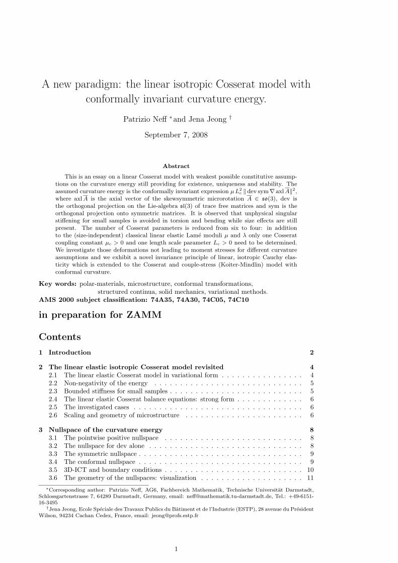
Si i d dSize independantclassical elasticity

Additional coarsegrid interaction due to curvature

Lcenergy

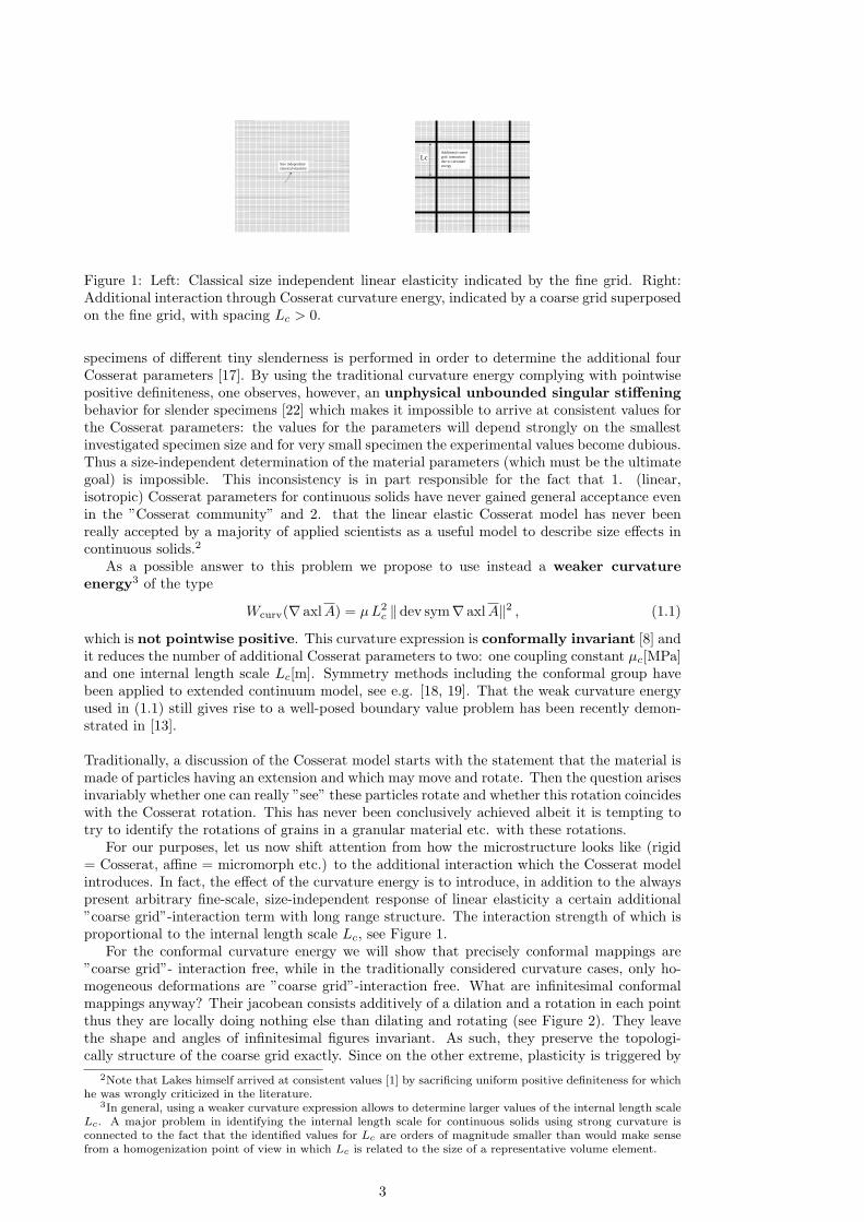
Figure 1: Left: Classical size independent linear elasticity indicated by the fine grid. Right:Additional interaction through Cosserat curvature energy, indicated by a coarse grid superposedon the fine grid, with spacing Lc > 0.

specimens of different tiny slenderness is performed in order to determine the additional fourCosserat parameters [17]. By using the traditional curvature energy complying with pointwisepositive definiteness, one observes, however, an unphysical unbounded singular stiffeningbehavior for slender specimens [22] which makes it impossible to arrive at consistent values forthe Cosserat parameters: the values for the parameters will depend strongly on the smallestinvestigated specimen size and for very small specimen the experimental values become dubious.Thus a size-independent determination of the material parameters (which must be the ultimategoal) is impossible. This inconsistency is in part responsible for the fact that 1. (linear,isotropic) Cosserat parameters for continuous solids have never gained general acceptance evenin the ”Cosserat community” and 2. that the linear elastic Cosserat model has never beenreally accepted by a majority of applied scientists as a useful model to describe size effects incontinuous solids.2

As a possible answer to this problem we propose to use instead a weaker curvatureenergy3 of the type

Wcurv(∇ axlA) = µL2c ‖ dev sym∇ axlA‖2 , (1.1)

which is not pointwise positive. This curvature expression is conformally invariant [8] andit reduces the number of additional Cosserat parameters to two: one coupling constant µc[MPa]and one internal length scale Lc[m]. Symmetry methods including the conformal group havebeen applied to extended continuum model, see e.g. [18, 19]. That the weak curvature energyused in (1.1) still gives rise to a well-posed boundary value problem has been recently demon-strated in [13].

Traditionally, a discussion of the Cosserat model starts with the statement that the material ismade of particles having an extension and which may move and rotate. Then the question arisesinvariably whether one can really ”see” these particles rotate and whether this rotation coincideswith the Cosserat rotation. This has never been conclusively achieved albeit it is tempting totry to identify the rotations of grains in a granular material etc. with these rotations.

For our purposes, let us now shift attention from how the microstructure looks like (rigid= Cosserat, affine = micromorph etc.) to the additional interaction which the Cosserat modelintroduces. In fact, the effect of the curvature energy is to introduce, in addition to the alwayspresent arbitrary fine-scale, size-independent response of linear elasticity a certain additional”coarse grid”-interaction term with long range structure. The interaction strength of which isproportional to the internal length scale Lc, see Figure 1.

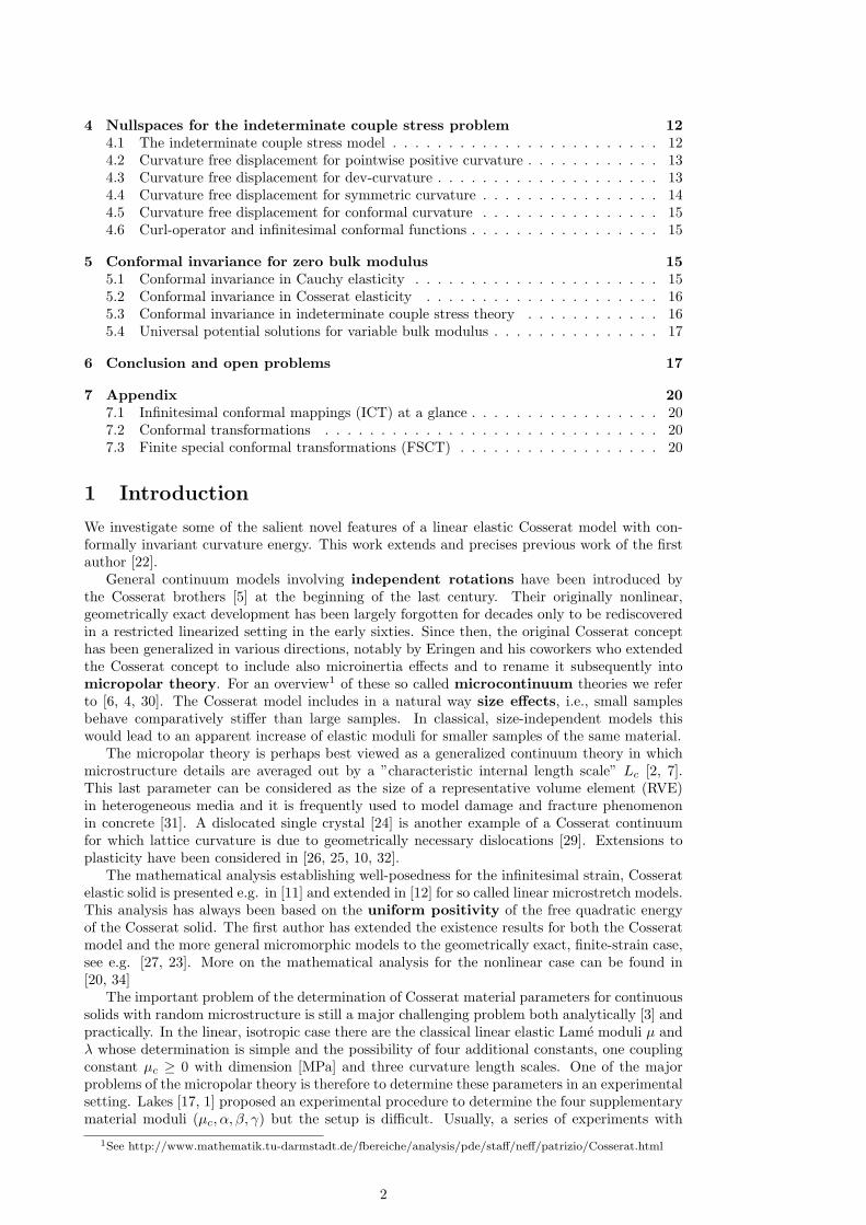
For the conformal curvature energy we will show that precisely conformal mappings are”coarse grid”- interaction free, while in the traditionally considered curvature cases, only ho-mogeneous deformations are ”coarse grid”-interaction free. What are infinitesimal conformalmappings anyway? Their jacobean consists additively of a dilation and a rotation in each pointthus they are locally doing nothing else than dilating and rotating (see Figure 2). They leavethe shape and angles of infinitesimal figures invariant. As such, they preserve the topologi-cally structure of the coarse grid exactly. Since on the other extreme, plasticity is triggered by

2Note that Lakes himself arrived at consistent values [1] by sacrificing uniform positive definiteness for whichhe was wrongly criticized in the literature.

3In general, using a weaker curvature expression allows to determine larger values of the internal length scaleLc. A major problem in identifying the internal length scale for continuous solids using strong curvature isconnected to the fact that the identified values for Lc are orders of magnitude smaller than would make sensefrom a homogenization point of view in which Lc is related to the size of a representative volume element.

3

0.0 0.5 1.0 1.5

-0.5

0.0

0.5

1.0

0.0 0.5 1.0 1.5 2.0

-1.0

-0.5

0.0

0.5

1.0

-0.5 0.0 0.5 1.0 1.5 2.0 2.5

0.0

0.5

1.0

1.5

2.0

2.5

3.0

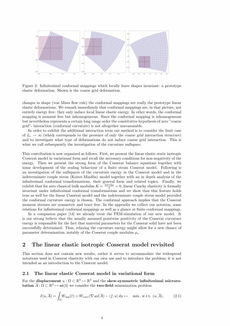
Figure 2: Infinitesimal conformal mappings which locally leave shapes invariant: a prototypeelastic deformation. Shown is the coarse grid deformation.

changes in shape (von Mises flow rule) the conformal mappings are really the prototype linearelastic deformations. We remark immediately that conformal mappings are, in that picture, notentirely energy free: they only induce local linear elastic energy. In other words, the conformalmapping is moment free but inhomogeneous. Since the conformal mapping is inhomogeneousbut nevertheless represents a certain long range order the constitutive hypothesis of zero ”coarsegrid”- interaction (conformal curvature) is not altogether unreasonable.

In order to exhibit the additional interaction term our method is to consider the limit caseof Lc → ∞ (which corresponds to the presence of only the coarse grid interaction structure)and to investigate what type of deformations do not induce coarse grid interaction. This iswhat we call subsequently the investigation of the curvature nullspace.

This contribution is now organized as follows. First, we present the linear elastic static isotropicCosserat model in variational form and recall the necessary conditions for non-negativity of theenergy. Then we present the strong form of the Cosserat balance equations together withsome development of the scaling behaviour of a finite strain Cosserat model. Following isan investigation of the nullspaces of the curvature energy in the Cosserat model and in theindeterminate couple stress (Koiter-Mindlin) model together with an in depth analysis of theinfinitesimal conformal transformations, their general form and related topics. Finally, weexhibit that for zero classical bulk modulus K = 3λ+2µ

3 = 0, linear Cauchy elasticity is formallyinvariant under infinitesimal conformal transformations and we show that this feature holdstrue as well for the linear Cosserat model and the indeterminate couple stress model providedthe conformal curvature energy is chosen. The conformal approach implies that the Cosseratmoment stresses are symmetric and trace free. In the appendix we collect our notation, somerelations for infinitesimal conformal mappings as well as a glance at finite conformal mappings.

In a companion paper [14] we already treat the FEM-simulation of our new model. Itis our strong believe that the usually assumed pointwise positivity of the Cosserat curvatureenergy is responsible for the fact that material parameters for the Cosserat solid have not beensuccessfully determined. Thus, relaxing the curvature energy might allow for a new chance ofparameter determination, notably of the Cosserat couple modulus µc.

2 The linear elastic isotropic Cosserat model revisited

This section does not contain new results, rather it serves to accommodate the widespreadnotations used in Cosserat elasticity with our own use and to introduce the problem; it is notintended as an introduction to the Cosserat model.

2.1 The linear elastic Cosserat model in variational form

For the displacement u : Ω ⊂ R3 7→ R3 and the skew-symmetric infinitesimal microro-tation A : Ω ⊂ R3 7→ so(3) we consider the two-field minimization problem

I(u,A) =∫

Ω

Wmp(ε) +Wcurv(∇ axlA)− 〈f, u〉dx 7→ min . w.r.t. (u,A), (2.1)

4

under the following constitutive requirements and boundary conditions

ε = ∇u−A, first Cosserat stretch tensor

u|Γ = ud , essential displacement boundary conditions

Wmp(ε) = µ ‖ sym ε‖2 + µc ‖ skew ε‖2 +λ

2tr [sym ε]2 strain energy

φ := axlA ∈ R3, k = ∇φ , ‖ curlφ‖2R3 = 4‖ axl skew∇φ‖2R3 = 2‖ skew∇φ‖2M3×3 ,

Wcurv(∇φ) =γ + β

2‖ dev sym∇φ‖2 +

γ − β2‖ skew∇φ‖2 +

3α+ (β + γ)6

tr [∇φ]2 . (2.2)

Here, f are given volume forces while ud are Dirichlet boundary conditions for the displacementat Γ ⊂ ∂Ω. Surface tractions, volume couples and surface couples could be included in thestandard way. The strain energy Wmp and the curvature energy Wcurv are the most generalisotropic quadratic forms in the infinitesimal non-symmetric first Cosserat strain tensorε = ∇u − A and the micropolar curvature tensor k = ∇ axlA = ∇φ (curvature-twisttensor). The parameters µ, λ[MPa] are the classical size-independent Lame moduli and α, β, γare additional micropolar moduli with dimension [Pa ·m2] = [N] of a force. The additionalparameter µc ≥ 0[MPa] in the strain energy is the Cosserat couple modulus which ideallyshould be size-independent as well. For µc = 0 the two fields of displacement and microrotationsdecouple and one is left formally with classical linear elasticity for the displacement u.

Remark 2.1 (Boundary conditions for the Cosserat model)It is always possible to prescribe essential boundary values for the microrotations A but weabstain from such a prescription because the physical meaning of it is doubtful. Similarly,surface couples are not prescribed. Note that well-posedness of the Cosserat model is true forfree-Neumann-type conditions on the microrotation anyway. Therefore, any artificial boundaryrequirement will heavily influence the solution.

2.2 Non-negativity of the energy

The condition for non-negativity of the energy are well known [22]. It must hold

µ ≥ 0 , µc ≥ 0 , 2µ+ 3λ ≥ 0 ,γ + β ≥ 0 , γ − β ≥ 0 , 3α+ (β + γ) ≥ 0 . (2.3)

Certain of these inequalities need to be strict in order for the well-posedness of the model.However, the uniform pointwise positivity (strict inequalities everywhere) is not necessary [13],although it is assumed most often in treatments of linear Cosserat elasticity [30].

2.3 Bounded stiffness for small samples

For every physical material, it is essential that small samples still show bounded rigidity. How-ever, this may or may not be true for Cosserat models, depending on the values of Cosseratparameters. Based on analytic solution formulas for simple three-dimensional Cosserat bound-ary value problems it has been shown in [22] that for bounded stiffness for arbitrary slendercylindrical samples we must have

1. in torsion of a slender cylinder: β + γ = 0 or Ψ = β+γα+β+γ = 3

2 .

2. in bending of a slender cylinder: (β + γ) (γ − β) = 0.

The conformal curvature energy (1.1) satisfies both requirements through β = γ and Ψ = 32 .4

We note that bounded stiffness does not imply that there is no size effect. Rather, it boundsthe size-effect away from unphysical limits.

4The additional conditions in [22] for bounded stiffness have been based on dimensionally reduced modelsand must therefore be taken with care.

5

2.4 The linear elastic Cosserat balance equations: strong form

The induced balance equations are

Div σ = f , balance of linear momentum

−Divm = 4µc · axl skew ε , balance of angular momentum (2.4)σ = 2µ · sym ε+ 2µc · skew ε+ λ · tr [ε] · 11 ,m = γ∇φ+ β∇φT + α tr [∇φ] · 11 , φ = axlA , u|Γ = ud .

Here, m is the (second order) couple stress tensor which is given as a linear function of thecurvature ∇φ = ∇ axlA and σ is the non-symmetric force stress tensor.

2.5 The investigated cases

We run the Cosserat model with basically three different sets of variables for the curvatureenergy which in each step relaxes the curvature energy. The cases are

1: pointwise positive case: µL2c

2 ‖∇φ‖2. This corresponds to α = 0, β = 0, γ = µL2

c .Eringen notes [6, p.151]: ”often it is assumed that γ is the leading term and α, β areestimated to be small, non-negative quantities.” In the linear setting this case can bearrived at by homogenization of materials with periodic microstructure like grid worksand lattice beams, see again [6].

1.1: deviatoric case: µL2c

2 ‖ dev∇φ‖2 = µL2c

2 (‖∇φ‖2 − 13 tr [∇φ]2). This corresponds to β =

0 and γ = µL2c

2 and α = − 13µL

2c . This is the second case of Lakes [17]. Note that

interpreting the coefficient α here as a ”spring-constant” is impossible, since α takesnegative values while the curvature energy is still positive semi-definite. The same remarkapplies, with appropriate changes, to case three.

2: symmetric case: µL2c

2 ‖ sym∇φ‖2. This corresponds to α = 0, β = γ and γ = µL2c

2 . In[36, 35] it is proposed to use β = γ based on non-standard curvature invariance principle.It leads already to a symmetric couple stress tensor m. The same requirement,based on another motivation has been arrived at in [33].

3: conformal case: µL2c

2 ‖ dev sym∇φ‖2 = µL2c

2 (‖ sym∇φ‖2 − 13 tr [∇φ]2). This corresponds

to β = γ and γ = µL2c

2 and α = − 13µL

2c . This is the first case of Lakes and our conformal

curvature. Here, the Cosserat couple stress tensor m is symmetric and trace free. For theindeterminate couple-stress problem (4.1) the last two cases coincide since the trace termis cancelled.

The reader should realize that all these cases are well-posed. The well-posedness of the last caseis a new result, proved in [13], making use of a new coercive inequality for formally positivequadratic forms. The well-posedness in the second case is a consequence of Korn’s secondinequality applied to the curvature energy. The first case is representative of a pointwisepositive curvature energy and therefore deserves no further comment. The first subcase can besubsumed in the third case.

Remark 2.2In a plain-strain, two-dimensional setting the axis of rotations is constant and all these curvaturecases coincide. This underlines the fact that the Cosserat model is essentially three-dimensional.

2.6 Scaling and geometry of microstructure

By a simple scaling argument one may see that very small samples of a material can be describedby the Cosserat model with increased Lc. In this sense, Lc → ∞ corresponds to arbitrarysmall samples. Let us present the scaling relations appearing in a finite-strain elastic Cosserattheory. We consider a finite-strain Cosserat model because the scaling relations are much moretransparent then. Our goal is to relate the response of large and small samples of the samematerial and to asses the influence of the characteristic length Lc.

6

L!" # $ ˆ.Lu B% %!"

&L!" # $

LL % %

!"

# $ # $ # $ # $22 2 2RVE' # $ # $ # $ # $22 2 2

L

RVEL c Lsym u L D u dV

%

( % ( % %)"

* +' ! ! ! !

1!" # $ ˆ.u x B x%1!" # $1!"

&&

2RVEL' () # $ # $ # $

1

2 2 2c

x

Lsym u x D u x dV xL

* *+"

' (, - . /0 1) ! ! ! !

1

Figure 3: Scaling relations and homogeneous boundary conditions.

First, we define the characteristic length LRVEc as given material parameter, correspond-

ing to the smallest discernible distance to be accounted for in the model. A simple conse-quence is that actual geometrical dimensions L of the bulk material must be larger than LRVE

c ,indeed for a continuum theory to apply at all L should be significantly larger than LRVE

c . Wemay thus identify LRVE

c with the size of a representative volume element RVE. The classicalsize-independent model ensues if L is arbitrary larger than LRVE

c in which we have separationof scales.

Now let ΩL = [0, L[m]]× [0, L[m]]× [0, L[m]] be the cube with (non-dimensional) edge lengthL, representing the bulk material. Consider a deformation ϕL : ξ ∈ ΩL 7→ R3 and microrotationRL(ξ) : ΩL 7→ SO(3) as solution of the generic (µc = µ) minimization problem∫ξ∈ΩL

µ(ξ) ‖RTL(ξ)FL(ξ)− 11‖2 + µ (LRVEc )2 ‖DξRL(ξ)‖2 dξ 7→ min . w.r.t. (ϕL, RL) , (2.5)

subject to homogeneous boundary conditions ξ ∈ ∂ΩL : ϕL(ξ) = (11 + B).ξ , B ∈ gl(3) .

This is the finite-strain problem which corresponds to the infinitesimal Cosserat model in vari-ational form∫ξ∈ΩL

µ(ξ) ‖ sym∇ξuL(ξ)‖2 + µ(ξ) ‖ skew∇ξuL(ξ)−AL(ξ)‖2

+ µ (LRVEc )2 ‖DξAL(ξ)‖2 dξ 7→ min . w.r.t. (uL, AL) , (2.6)

subject to homogeneous boundary conditions ξ ∈ ∂ΩL : uL(ξ) = B.ξ , B ∈ gl(3) .

The simple scaling transformation ζ : R3 7→ R3, ζ(x) = L · x maps the unit cube Ω1 =[0, 1[m]] × [0, 1[m]] × [0, 1[m]] into ΩL. Defining the related deformation ϕ : x ∈ Ω1 7→ R3 andmicrorotation R(x) : Ω1 7→ SO(3) as

ϕ(x) := ζ−1 (ϕL(ζ(x))) , R(x) := RL(ζ(x)) , (2.7)

shows

∇xϕ(x) =1L∇ξϕL(ζ(x))∇xζ(x) = ∇ξϕL(ξ) ,

DxR(x) = DξRL(ζ(x)) · ∇xζ(x) = DξRL(ξ) · L ,

ϕ(x) =1LϕL(L · x) = (11 + B).x , x ∈ ∂Ω1 . (2.8)

Hence, the minimization problem can be transformed to the unit cube5∫ξ∈ΩL

µ(ξ) ‖RTL(ξ)∇ξϕL(ξ)− 11‖2 + µ L2c ‖DξRL(ξ)‖2 dξ

=∫x∈Ω1

µ(Lx) ‖RT (x)∇xϕ(x)− 11‖2 det[∇xζ(x)] + µ (LRVEc )2 ‖ 1

LDxR(x)‖2 det[∇xζ(x)] dx

5Homogeneous boundary conditions are invariant under the re-scaling, as is any one-homogeneous expressionϕL(r ξ) = r ϕL(ξ) as e.g., ϕL(ξ) = B.ξ + ξ⊗ξ

‖ξ‖ .b.

7

=∫x∈Ω1

µ(Lx) ‖RT (x)∇xϕ(x)− 11‖2 L3 + µ (LRVEc )2 L3−2 ‖DxR(x)‖2 dx , (2.9)

and dividing by L3 we may consider at last the equivalent problem defined on the unit cubeΩ1:∫x∈Ω1

µ(Lx) ‖RT (x)∇xϕ(x)− 11‖2 + µ(LRVE

c )2

L2‖DxR(x)‖2 dx 7→ min . w.r.t. (ϕ,R).

still subject to homogeneous boundary conditions x ∈ ∂Ω1 : ϕ(x) = (11 + B).x , B ∈ gl(3) .

Thus we are led to define a relative internal length Lc := (LRVEc )2

L2 , which is in fact that Lc whichwe use in this work most of the time. Comparison of different sample sizes is now afforded bytransformation to the unit cube respectively, e.g., we compare two samples of the same materialwith bulk sizes L1 > L2. Transformation to the unit cube shows that the response of sampleΩL2 is stiffer than the response of sample ΩL1 . It is plain to see that for L large compared toLRVEc , the influence of the rotations will be small and in the limit LRVE

c

L → 0, classical, size-

independent behaviour results. Otherwise, the larger LRVEc

L , the more pronounced the Cosserateffects become and a small sample is relatively stiffer than a large one.

For a very small cube ΩL with side length L 1 we have Lc = LRVEc

L 1. Consider therefore(hypothetically) the limit Lc → ∞. In a variational context the energy has to remain finite.In case Lc = ∞ it is understood that Wcurv must vanish. Therefore, the precise form ofthe curvature energy determines, which deformation possibilities remain for the substructureitself. These deformation possibilities are given by the nullspace of the curvature contribution.The nullspace of the curvature determines therefore the ”coarse grid”-interaction law. Thehypothetical limit Lc →∞ therefore characterizes completely the interaction which is inducedby the presence of a microstructure which induces a ”coarse-grid” setting. Thus we investigatethe null-space now.

3 Nullspace of the curvature energy

Since we are interested in the response of the Cosserat model primarily with respect to differentcurvature energies it is next expedient to investigate the nullspaces of the respective expressions.In the following, constant terms are denoted with a hat by W , A ∈ so(3), b ∈ R3, p ∈ R etc.

3.1 The pointwise positive nullspace

The first case 1 is simple. In the following we abbreviate with φ : R3 7→ R3 the axial vector ofthe microrotation A ∈ so(3), i.e. φ = axlA. Subsequently, when there is no danger of confusion,we use A also to denote an arbitrary skew-symmetric matrix.

The condition of zero curvature energy µL2c ‖∇φ‖2 = 0 is simply ∇φ = 0 and this implies

φ(x1, x2, x3) := b , (3.1)

for some constant translational vector b ∈ R3. This is the three-dimensional space of transla-tions. It implies strong stiffening behaviour as Lc →∞ which is also observed in our simulationsin the companion paper [14] together with the solution for Lc =∞.

Remark 3.1 (Boundary conditions)If A = 0 (equivalently φ = 0) at Γ ⊂ ∂Ω for (3.1) then A ≡ 0 (φ ≡ 0) in Ω. In fact, forsmooth fields, it suffices to prescribe φ = 0 at an isolated point only.

3.2 The nullspace for dev alone

The first subcase 1.1 is also simple. The condition of zero curvature energy is dev∇φ = 0 andthis implies ∇φ = p(x) 11 for some scalar field p : Ω ⊂ R3 7→ R. Taking the Curl on both sidesof the last equation yields

0 = Curl[p(x) 11] =

0 px3 −px2

−px3 0 px1

px2 −px1 0

∈ so(3) . (3.2)

8

Thus ∇p(x) = 0 and we have after integration

φ(x1, x2, x3) := p x+ b , (3.3)

for some constant translational vector b ∈ R3 and a constant number p ∈ R. This is a four-dimensional space. The decisive new feature as compared to (3.1) is that now a linear variationof microrotations does not necessarily lead to curvature energy or moment stresses. This willalso obtain in the next case.

Remark 3.2 (Boundary conditions)If A = 0 (φ = 0) at Γ ⊂ ∂Ω for (3.3) then A ≡ 0 (φ ≡ 0) in Ω. In fact, for smooth fields, itsuffices to prescribe φ = 0 on a one-dimensional curve.

3.3 The symmetric nullspace

In the second symmetric curvature situation, case 2, we obtain from the zero curvature require-ment that sym∇φ = 0 which locally means

∇φ(x1, x2, x3) = A(x1, x2, x2) ∈ so(3) ⇒ 0 = CurlA(x1, x2, x2) ⇒ A(x) = A = const. , (3.4)

on using formula (3.6)4. This implies that

φ(x1, x2, x3) := A.x+ b , (3.5)

where A ∈ so(3) and b ∈ R3 are some constant skew-symmetric matrix and constant translation,respectively. This is the well known six-dimensional space of infinitesimal rigid movements. Letus collect some useful formulas for this case (three space dimensions):

−CurlA = [∇ axlA]T − tr[∇ axlA

]11 , tr

[CurlA

]= 2 tr

[∇ axlA

],

‖CurlA‖2 = ‖∇ axl(A)‖2 + tr[∇ axlA

]2 ≥ ‖∇ axl(A)‖2 ,− sym CurlA = sym[∇ axlA]− tr

[∇ axlA

]11 ,

‖ sym CurlA‖2 = ‖ sym∇ axl(A)‖2 + tr[∇ axlA

]2. (3.6)

The last equality suggest that the parameter values β = γ = α could also be an interestingconstitutive choice. Inequality (3.6)2 admits a (surprising) generalization to exact rotations[28]. Considering the deviator, we observe, moreover

‖dev sym CurlA‖2 = ‖ sym CurlA‖2 − 13

tr[CurlA

]2= ‖ sym∇ axl(A)‖2 + tr

[∇ axlA

]2 − 13

tr[CurlA

]2= ‖ sym∇ axl(A)‖2 + tr

[∇ axlA

]2 − 43

tr[∇ axlA

]2= ‖ sym∇ axl(A)‖2 − 1

3tr[∇ axlA

]2= ‖ dev sym∇ axlA‖2 . (3.7)

Remark 3.3 (Boundary conditions)If A = 0 (φ = 0) at Γ ⊂ ∂Ω for (3.5) then A ≡ 0 (φ ≡ 0) in Ω. This result follows as inlinear elasticity for the displacement. Here it is decisive that Γ is a two-dimensional surface,otherwise the infinitesimal rotations are not fixed.

3.4 The conformal nullspace

In the last case 3 we obtain for vectorfields φ : R3 7→ R3 the condition dev sym∇φ = 0. Onecan show that the nullspace in dimension n ≥ 3 has dimension (n + 1) (n + 2)/2.6 To see this

6In dimension n = 2 the kernel is infinite-dimensional. Consider

∇φ(x) =

„φ1,x1 φ1,x2φ2,x1 φ2,x2

«=

„ bp ba−ba bp

«⇒ dev2 sym∇φ = 0 . (3.8)

Thus φ1, φ2 satisfy the Cauchy-Riemann equations and all harmonic functions are in the kernel.

9

for dimension n = 3, consider that dev sym∇φ = 0 implies ∇φ = p(x) 11 + A(x) for a scalarfield p : Ω 7→ R and a skew-symmetric field A : Ω 7→ so(3). Taking the Curl yields

∇φ = p(x) 11 +A(x) ⇒ 0 = Curl[p(x) 11]︸ ︷︷ ︸∈so(3), (3.2)

+ CurlA(x) ⇒

0 = sym CurlA(x) ⇒︸︷︷︸(3.6)4

sym∇ axl(A(x)) = 0 ⇒

∇ axl(A(x)) = W (x) ∈ so(3) ⇒ axl(A(x)) = W .x+ η ⇒ (3.9)

−CurlA = [∇ axlA]T − tr[∇ axlA

]11 = WT − 0 ⇒ Curl[p(x) 11] = WT = −W ⇒

Curl[p(x) 11] =

0 px3 −px2

−px3 0 px1

px2 −px1 0

= −W ⇒ ∇p =

px1

px2

px3

=

−W23

W13

−W12

= axl(W ) .

Integration yields p(x) = 〈axl(W ), x〉+ p, which implies

∇φ = p(x) 11 +A(x) = [〈axl(W ), x〉+ p] 11 + anti(W .x+ η)

= [〈axl(W ), x〉+ p] 11 + anti(W .x) + A = anti(W .x) + 〈axl(W ), x〉 11 + [p 11 + A] ⇒

φ =12

(2〈axl(W ), x〉x− axl(W ) ‖x‖2

)+ [p 11 + A].x+ b . (3.10)

We have thus shown that for n = 3 the kernel is ten-dimensional.7 It consists of all infinitesi-mal conformal transformations (ICT) having the form (abbreviate k = 1

2 axl(W ))

φC(x1, x2, x3) : =3∑i=1

ki Qi(x, x) + M.x+ b = 2〈k, x〉 − k ‖x‖2 + M.x+ b , M = p 11 + A ,

∇φC(x1, x2, x3) = 2 [anti(W .x) + 〈axl(W ), x〉 11] + M , (3.11)

D2φC(x).h = 2 [anti(W .h) + 〈axl(W ), h〉 11] ∈ R 11⊕ so(3) ,

where p, k1, k2, k3 ∈ R and A ∈ so(3) and b are constant numbers, constant skew-symmetricmatrix and constant translation, respectively. Here, Qi : R3×R3 7→ R3 are three infinitesimalspecial conformal transformations (ISCT) (which we have shown to be second orderpolynomials):

Q1(x, x) := 2x1

x1

x2

x3

−‖x‖20

0

=

x21 − (x2

2 + x23)

2x1x2

2x1x3

, ∇Q1(x, x) = 2

x1 −x2 −x3

x2 x1 0x3 0 x1

,

Q2(x, x) := 2x2

x1

x2

x3

− 0‖x‖2

0

=

2x1 x2

x22 − (x2

1 + x23)

2x2x3

, ∇Q2(x, x) = 2

x2 x1 0−x1 x2 −x3

0 x3 x2

,

Q3(x, x) := 2x3

x1

x2

x3

− 0

0‖x‖2

=

2x3 x1

2x3 x2

x23 − (x2

1 + x22)

, ∇Q3(x, x) = 2

x3 0 x1

0 x3 x2

−x1 −x2 x3

(3.12)

It is easy to check that ∇Qi = p(x) 11 + A(x) for A(x) ∈ so(3) and p(x) ∈ R. A short formrepresentation is given by

Qi(x, x) = 2〈x, ei〉x− ‖x‖2 ei . (3.13)

3.5 3D-ICT and boundary conditions

Let us show that infinitesimal conformal transformations (ICT), while offering richer possibili-ties than rigid movements, are still uniquely determined when set to zero on a two-dimensionalsmooth surface Γ. More precisely, we show

7It is plain to see that φC forms a ten-dimensional linear space which can be endowed with the structure ofa Lie-algebra by using as Lie-bracket the usual commutator bracket for vectorfields.

10

Lemma 3.4If A = 0 (φ = 0) at Γ ⊂ ∂Ω for (3.11) then A ≡ 0 (φ ≡ 0) in Ω.

Proof. We choose curves γi : R 7→ Γ ⊂ R3 which lie on the surface Γ. Along these curves itholds by assumption that

φ(γ(t)) = 0 ⇒ 0 =ddtφ(γ(t)) = ∇φ(γ(t)).γ′(t) . (3.14)

Since we can always choose curves which pass through a given point γ(t0) = x0 ∈ Γ and since Γis a smooth two-dimensional surface, there exist always two-linear independent directions τ1, τ2such that

∇φ(x0).τi = 0 , τi = γi′(t0) , i = 1, 2, γ(t0) = x0 . (3.15)

Therefore, we conclude that if φ = 0 on Γ then the rank of ∇φ is maximally one on Γ. On theother hand, φ being infinitesimal conformal, we have

∇φ(x0) = anti(W .x0) + 〈axl(W ), x0〉 11 + [p 11 + A]

= anti(W .x0) + A+ [〈axl(W ), x0〉+ p] 11 . (3.16)

Let us check the rank of this expression on Γ. Since it has the form ∇φ = so(3) + R · 11 we onlyhave to show that there exists an x0 ∈ Γ at which not both summands vanish simultaneously.This suffices since, if either of them is nonzero, then the rank is at least two: if only the skewsymmetric part vanishes then the rank is three, if only the dilation (spherical) part vanishes,then the rank is two.

Individually, if both vanish, we have

〈axl(W ), x0〉 = −p , 0 = anti(W .x0) + A ⇒ W .x0 = − axl(A) . (3.17)

In matrix form (axl(W )T

W

)x0 =

(−p

− axl(A)

)R4

. (3.18)

The first case is W = 0. Then p and A are both zero, which implies φ ≡ 0. In the second caseassume now that W 6= 0. A simple calculation shows that

rank

(axl(W )T

W

)3×4

= 3 ⇔ W 6= 0 . (3.19)

Thus the solution of (3.18) is given by

x0 = xinhom + s · xhom , s ∈ R , (3.20)

which parameterizes a straight line, but Γ is two-dimensional; the contradiction.

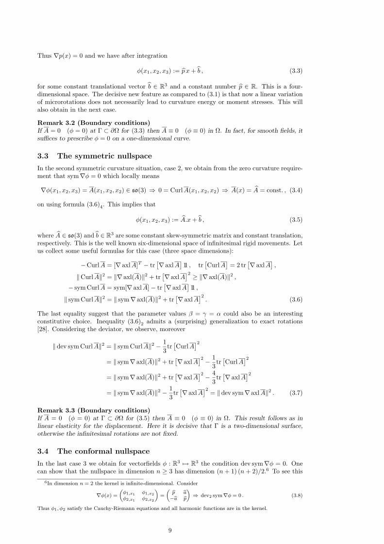
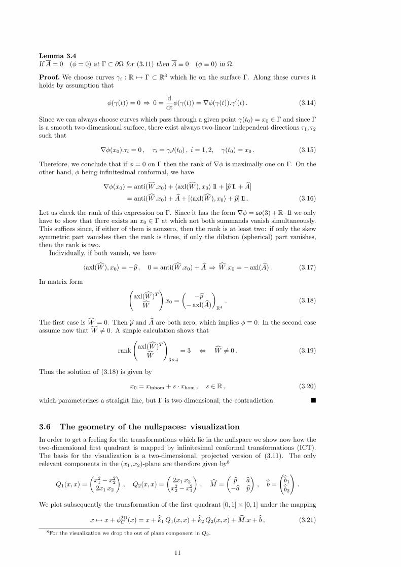
3.6 The geometry of the nullspaces: visualization

In order to get a feeling for the transformations which lie in the nullspace we show now how thetwo-dimensional first quadrant is mapped by infinitesimal conformal transformations (ICT).The basis for the visualization is a two-dimensional, projected version of (3.11). The onlyrelevant components in the (x1, x2)-plane are therefore given by8

Q1(x, x) =(x2

1 − x22

2x1 x2

), Q2(x, x) =

(2x1 x2

x22 − x2

1

), M =

(p a−a p

), b =

(b1b2

).

We plot subsequently the transformation of the first quadrant [0, 1]× [0, 1] under the mapping

x 7→ x+ φ2DC (x) = x+ k1Q1(x, x) + k2Q2(x, x) + M.x+ b , (3.21)

8For the visualization we drop the out of plane component in Q3.

11

0.0 0.2 0.4 0.6 0.8 1.0 1.2 1.4

0.0

0.2

0.4

0.6

0.8

1.0

1.2

1.4

0.0 0.2 0.4 0.6 0.8 1.0 1.2 1.4

-0.4

-0.2

0.0

0.2

0.4

0.6

0.8

1.0

Figure 4: Left: Mappings in the nullspace for dev alone. In this case, apart for theubiquitous constant translation vector b ∈ R3, we have p 6= 0 but a = 0, k1, k2 = 0. Thefirst quadrant is homogeneously scaled with p. Here p = 0.5. Right: Mappings inthe symmetric nullspace. Here, the transformation possibilities are encoded by a 6= 0 butp = 0, k1, k2 = 0. The first quadrant is homogeneously rotated with infinitesimal rotationangle a = 0.5. Note that the infinitesimal rotation also leads to a homogeneous increase involume which is an artifact of the linear model. In any of these cases, the deformation ishomogeneous only!

for numbers k1, k2, p, a, b1, b2. The parameter a is the infinitesimal rotation angle, b is a simpletranslation and will therefore be neglected, p is the infinitesimal change in length and k1, k2

parametrize the two-dimensional inhomogeneous infinitesimal special conformal transformations(ISCT).

In Figure 4 and Figure 5 we show the encoded deformation possibilities. The mappings inthe nullspace for pointwise positive curvature can only shift the first quadrant by the constantvector b ∈ R3 and are therefore not visualized. Note that this is not the deformation of thesubstructure itself, since the transformation corresponds to the axial vector of the infinitesimalrotation of the substructure, i.e, A(x) = anti(φ(x)), but we use φ to show the transformation.

4 Nullspaces for the indeterminate couple stress problem

The indeterminate couple stress problem [21, 15] is characterized by the identification 12 curlu =

axlA = φ which can be formally obtained from the genuine Cosserat model by setting µc =∞.Since here the infinitesimal microrotations A cease to be an independent field the model has theadvantage of conceptional simplicity and improved physical transparency.9 We can completelycharacterize what type of displacement u does not induce curvature energy for the differentcurvature cases. This allows to us to understand what kind of ”torsional spring analogy” maybe implied by the respective curvatures. Let us recall this Koiter-Mindlin model, for simplicitywithout external loads.

4.1 The indeterminate couple stress model

For the displacement u : Ω ⊂ R3 7→ R3 we consider the one-field minimization problem

I(u) =∫

Ω

Wmp(∇u) +Wcurv(∇ curlu) dV 7→ min . w.r.t. u,

under the constitutive requirements and boundary conditions

Wmp(ε) = µ ‖ sym∇u‖2 +λ

2tr [sym∇u]2 , u|Γ = ud ,

Wcurv(∇ curlu) =γ + β

8‖ sym∇ curlu‖2 +

γ − β8‖ skew∇ curlu‖2 . (4.1)

In this limit model, the curvature parameter α, related to the spherical part of the (higher order)couple stress tensor m remains indeterminate, since tr [∇φ] = Div axlA = Div 1

2 curlu = 0. Amotivation for this model in a finite-strain, multiplicative elasto-plastic context has been given

9At the prize of being a fourth order boundary value problem.

12

0.0 0.5 1.0 1.5

-0.5

0.0

0.5

1.0

0.0 0.5 1.0 1.5 2.0

-1.0

-0.5

0.0

0.5

1.0

-0.5 0.0 0.5 1.0 1.5 2.0 2.5

0.0

0.5

1.0

1.5

2.0

2.5

3.0

Figure 5: Mappings in the conformal nullspace. Finally, in the conformal case we can varya, p, k1, k2. We plot the transformation of the first quadrant that does not induce curvatureenergy. If k2

1 + k22 > 0, then the first quadrant is inhomogeneously transformed. Clock

wise: homogeneous rotation and scaling with p = 0.2, a = 0.5, inhomogeneous mapping a =0, p = 0.6, k1 = 0.2, k2 = 0.4 and a = 0, p = 0.6, k1 = 0.8, k2 = 0.4. The effect of thecurvature energy is to introduce, in addition to the always present arbitrary fine-scale, size-independent response of linear elasticity a certain additional ”coarse grid”-interaction termwith long range structure. The interaction strength of which is proportional to Lc. For theconformal curvature energy, the conformal mappings are therefore ”coarse grid” interactionfree, while in the previous cases, only homogeneous deformations are ”coarse grid” interactionfree. Remark that the above mappings are not entirely energy free: they only induce local linearelastic energy. In other words, the conformal mapping is moment free but inhomogeneous. Sincethe conformal mapping is inhomogeneous but nevertheless represents a certain long range orderthe constitutive hypothesis of zero ”coarse grid” interaction is not altogether unreasonable.

recently in [9]. Following [15], it is practically always assumed that −1 < η := βγ < 1 in order

to guarantee uniform positive definiteness [3]. For the conformal case, we use, on the contraryβγ = 1, which makes the couple stress tensor symmetric and trace free. The curvature freedisplacements u are, by definition, those displacements that ”survive” in the limit of internallength scale Lc →∞ (i.e. γ + β →∞, γ − β →∞).

4.2 Curvature free displacement for pointwise positive curvature

This is the case where, formally, γ + β, γ − β > 0. Here, from ‖∇ curlu‖ = 0 it must hold for agiven constant vector b ∈ R3, see (3.1)

12

curlu = axlA(x) = b ⇒ curlu = 2 b ⇒ u(x) = ∇ζ(x) + anti(b).x+ ξ︸ ︷︷ ︸infinitesimal rigid movement

, (4.2)

We find the solution in the form u = uhom + uspec. The homogeneous solution curluhom = 0 isuhom = ∇ζ + ξ where ζ : R3 7→ R is a scalar potential and ξ ∈ R3 is another constant vector.One special solution of curlu = 2 b is given by uspec = anti(b).x since curlu = 2 axl(skew∇u).Altogether, the displacement gradient follows as

∇u(x) = D2ζ(x) + anti(b) . (4.3)

Hence, in the elastic energy only the symmetric part appears with energy

µ ‖ dev sym∇u(x)‖2 +K

2tr [∇u(x)]2 = µ ‖devD2ζ(x)‖2 +

K

2tr[D2ζ(x)

]2. (4.4)

Thus only the irrotational part contributes to the elastic energy and for Lc →∞ and−1 < η < 1the limit variational problem reduces to a second order energy on a scalar potential ζ.

4.3 Curvature free displacement for dev-curvature

Here, we consider the first subcase 1.1. Looking at (3.3) and using the identification 12 curlu =

axl(A) = φ we obtain for a given constant vector b ∈ R3 and a given constant number p

curlu = p x+ b ⇒ u(x) = ∇ζ(x) + anti(b).x+ ξ , (4.5)

13

where ζ : R3 7→ R is a scalar potential and ξ ∈ R3 is another constant vector. This casecoincides with the previous one! To see this, consider

curlu = p x+ b ⇒ 0 = Div curlu(x) = Div[p x] = tr [∇[p x]] = tr [p 11] = 3 p . (4.6)

Thus, p must be zero and we are back in the previous case.

4.4 Curvature free displacement for symmetric curvature

Here, for a given constant vector b ∈ R3 and a given constant skew-symmetric matrix A ∈ so(3)we must have (see (3.5))

curlu = A.x+ b ⇒ u(x) = ∇ζ(x) + P2(x) + anti(b).x+ ξ , (4.7)

where ζ : R3 7→ R is a scalar potential, ξ ∈ R3 is another constant vector and P2 : R3 7→ R3 isa homogeneous polynomial of second order such that

curlP2(x) = A.x . (4.8)

A simple calculation confirms the (for us at first surprising) result that for some constant vectorη ∈ R3, depending on the entries of A ∈ so(3), the polynomial P2 can be chosen as

P2(x) = 2〈η, x〉x− η ‖x‖2 . (4.9)

To see this, we compute the total differential of P2 for h ∈ R3

DP2(x).h = 2 〈η, h〉x+ 2 〈η, x〉h− 2 η 〈x, h〉 = 2 (x⊗ η + 〈η, x〉 11− η ⊗ x) .h= 2 (2 skew(x⊗ η) + 〈η, x〉 11) .h ⇒

∇P2(x) = 2 (2 skew(x⊗ η) + 〈η, x〉 11)curlP2(x) := 2 axl(skew∇P2) = 8 axl(skew(x⊗ η)) = 4 η × x = 4 anti(η).x , (4.10)

where we have used, in this order of appearance, that curlu = 2 axl(skew∇u) and axl(skew(a⊗b)) = − 1

2 a× b and axl(A)× x = A.x. Therefore, choosing η = 14 axl(A) shows the claim. The

polynomial P2 is nothing else than the infinitesimal special conformal transformation (ISCT).10

Regarding (4.7) we may always subsume the scalar potential to be given in the form ζ+ bp2 ‖x‖

2

by misuse of notation for ζ. Thus, the curvature free displacements in the indeterminate couplestress theory with symmetric curvature (symmetric moment stresses) are of the form

u(x) = ∇ζ(x) +12

(2〈axl(W ), x〉x− axl(W ) ‖x‖2

)+ [p 11 + A].x+ b︸ ︷︷ ︸

infinitesimal conformal mapping

, (4.11)

with arbitrary constant terms W , A ∈ so(3), b ∈ R3 and p ∈ R. The corresponding displacementgradient is given by

∇u(x) = D2ζ(x)︸ ︷︷ ︸∈Sym(3): irrotational

+ [〈axl(W ), x〉+ p] 11 + anti(W .x) + A︸ ︷︷ ︸conformal derivative

. (4.12)

Hence, in the elastic energy of the formal limit problem Lc = ∞ only the symmetric partappears with energy

µ ‖D2ζ(x) + sym∇P2(x)‖2 +λ

2tr[D2ζ(x) +∇P2(x)

]2(4.13)

= µ ‖ dev sym(D2ζ(x) +∇P2(x))‖2 +2µ+ 3λ

6tr[D2ζ(x) +∇P2(x)

]2= µ ‖ devD2ζ(x)‖2 +

K

2tr[D2ζ(x) + [〈axl(W ), x〉+ p] 11

]2.

Assuming the formal limit case of zero bulk-modulus K = 0, the elastic energy consists only ofµ ‖ devD2ζ‖2.

10Thus, the infinitesimal special conformal transformations φ can be equivalently characterized through thecondition curlφ = bA.x for arbitrary bA ∈ so(3)!

14

4.5 Curvature free displacement for conformal curvature

Here, we must have curlu = φ, where φ : R3 7→ R3 is just an infinitesimal conformal mapping(ICT), which is, because of (3.11) given as

φ(x) =12

(2〈axl(W ), x〉x− axl(W ) ‖x‖2

)+ [p 11 + A].x+ b ,

∇φ(x) = [〈axl(W ), x〉+ p] 11 + anti(W .x) + A , (4.14)

where W , A ∈ so(3) and b ∈ R3 and p are given constants. Consider

0 = Div curlu = Div φ = tr [∇φ] = 3 [〈axl(W ), x〉+ p] ⇒

∀x ∈ R3 : −p = 〈axl(W ), x〉 . (4.15)

The last equation determines x to lie on a plane with normal axl(W ) but x ∈ R3 is arbitrary.Since p and W are both constant, they must therefore vanish. Hence, curlu = A.x+b. Thus, theconformal case is indistinguishable from the symmetric case as far as the formal limit Lc =∞is concerned in the indeterminate couple stress problem.

4.6 Curl-operator and infinitesimal conformal functions

Let us note a remarkable property concerning the curl-operator and infinitesimal conformalfunctions (ICT). We have

Lemma 4.1 (Infinitesimal conformal functions are closed under curl)Let φ ∈ ICT be given. Then curlφ = A.x+ b ∈ ICT for some constant skew-symmetric matrix

A ∈ so(3) and some constant vector b.

Proof. We have derived a complete characterization of infinitesimal conformal functions ICTgiven in (3.11). With constant terms W , A ∈ so(3), p ∈ R, b ∈ R3 they have the form

φ(x) =12

(2〈axl(W ), x〉x− axl(W ) ‖x‖2

)+ [p 11 + A].x+ b ,

∇φ(x) = [〈axl(W ), x〉+ p] 11 + anti(W .x) + A . (4.16)

Thus, applying the curl-operator, we obtain

curlφ = 2 axl(skew(∇φ)) = 2 axl(anti(W .x) + A)) = 2 [W .x+ axl(A)] , (4.17)

so that curlφ is in fact an infinitesimal rigid movement since W ∈ so(3) and axl(A) ∈ R3.

5 Conformal invariance for zero bulk modulus

The infinitesimal conformal invariance of the curvature energy does, however, not imply that thefully Cosserat coupled problem has this invariance in general. However, infinitesimal conformalinvariance is true in one special formal case: the case of zero bulk modulus. Of course, standardengineering materials have positive bulk modulus K > 0, which is also necessary for the well-posedness. Here, we set formally K = 0 but we remark that composite man made materialsmay have small K or even K = 0 [16].11 Let us consider linear elasticity as a starting point.

5.1 Conformal invariance in Cauchy elasticity

Considering the free energy of linear, isotropic Cauchy elasticity in the form∫Ω

µ(x) ‖ dev sym∇u‖2 +K(x)

2tr [∇u]2 dx , (5.1)

11http://silver.neep.wisc.edu/ lakes/Poisson.html

15

we observe that in the formal limit of zero bulk modulus K = 2µ+3λ3 = 0 the energy is invariant

under the transformation u 7→ u+φ, whenever φ is an infinitesimal conformal mapping, because

dev sym∇(u+ φ) = dev sym∇u+ dev sym∇φ = dev sym∇u . (5.2)

Since the first, deviatoric term measures only change in shape it does not see those trans-formations, which, infinitesimally, do not change shape - precisely the infinitesimal conformalmappings φ ∈ ICT . Thus, for zero bulk modulus K = 0, displacements u which are infinitesi-mal conformal mappings, see Figure 5, do not contribute to the elastic energy at all on the linearelastic ”macroscopic level”. A similar conclusion has been reached in [19] for incompressibleisotropic linear elasticity with zero pressure.

5.2 Conformal invariance in Cosserat elasticity

We consider the free energy of linear, isotropic Cosserat elasticity for zero bulk modulus K = 0in the form∫

Ω

µ ‖dev sym∇u‖2 +µc2‖ curlu− 2 axlA‖2 + µL2

c ‖ dev sym∇ axlA‖2 dx . (5.3)

With our preparation we see now immediately, that this energy is invariant under the transfor-mation of displacement and microrotations through

(u, axlA) 7→ (u+ φ, axlA+12

curlφ) , (5.4)

for all φ ∈ ICT . The invariance of the first term is clear as in linear elasticity. For the thirdterm use Lemma 4.1 to note that 1

2 curlφ ∈ ICT . For the second coupling term observe that

curl(u+ φ)− 2[axlA+12

curlφ] = curlu− 2 axlA . (5.5)

5.3 Conformal invariance in indeterminate couple stress theory

We consider at last the free energy of the linear, isotropic indeterminate couple stress theoryfor zero bulk modulus K = 0 in the form∫

Ω

µ ‖ dev sym∇u‖2 +µL2

c

4‖ dev sym∇ curlu‖2 dx . (5.6)

As before this energy is invariant under the transformation

u 7→ u+ φ , (5.7)

exactly as linear elasticity is for zero bulk modulus.Surprisingly, therefore, conformal invariance for zero bulk modulus can also be obtained for

the indeterminate couple stress model and the genuine Cosserat model provided we choose theconformal curvature expression. The line of argument is therefore not, why a model should haveconformal invariance, but to realize that linear elasticity has it on the outset for a certain pa-rameter range, and, therefore, the hypothesis is not altogether unreasonable that the extendedcontinuum models should have it as well for the same parameter range! We summarize thesefindings in the novel

Postulate I: If an isotropic linear elastic solid (whether itbe linear Cauchy elastic or a more general linear extendedcontinuum model) with positive bulk modulus is (infinites-imally) conformally deformed then the elastic energy mustconsist only of a purely volumetric term.

In the companion paper [14] we use conformal invariance to obtain inhomogeneous analyticalsolutions for boundary value problems in Cosserat elasticity.

16

5.4 Universal potential solutions for variable bulk modulus

Consider linear, isotropic Cauchy elasticity with constant shear modulus µ and variable bulkmodulus K(x): ∫

Ω

µ ‖dev sym∇u‖2 +K(x)

2tr [∇u]2 dx 7→ min . u

u|Γ(x) = ∇ζ(x) , ζ : R3 7→ R , ∆ζ = 0 , (5.8)

where ζ is a given harmonic function. This problem has a unique solution irrespective of thevariation of the bulk modulus K(x) and the solution is u(x) ≡ ∇ζ(x). We see this from

σ = 2µ dev sym∇u+K(x) tr [∇u]11 = 2µ (sym∇u− 13

tr [∇u]11) +K(x) tr [∇u]11

= 2µ sym∇u+ (K(x)− 2µ3

) tr [∇u]11 = µ (∇u+∇uT ) + (K(x)− 2µ3

) Div u 11 ,

Div σ = µ∆u+ µ∇Div u+ Div(K(x)− 2µ3

) Div u 11)

= µ∆u+ µ∇Div u+∇(K(x)− 2µ3

) Div u)

= µ∆u+∇(

(µ+ (K(x)− 2µ3

)) Div u)

= µ∆u+∇(

(K(x) +µ

3) Div u

). (5.9)

For u = ∇ζ we have Div u = ∆ζ = 0. Moreover,

∆u =

∆u1

∆u2

∆u3

=

∆(∇ζ)1

∆(∇ζ)2

∆(∇ζ)3

=

∆ζx∆ζy∆ζz

=

(∆ζ)x(∆ζ)y(∆ζ)z

=

000

. (5.10)

Thus Div σ = 0 and the boundary conditions are trivially satisfied. It is clear that the sameholds true for the general Cosserat and the indeterminate couple stress problem since by theappearance of curlu in both models, the term ∇ζ will be annihilated.

We turn this result as well into a novel requirement

Postulate II: If an isotropic linear elastic solid (whether itbe linear Cauchy elastic or a more general linear extendedcontinuum model) is subject to harmonic gradient Dirichletboundary conditions u|Γ(x) = ∇ζ(x) , ζ : R3 7→ R , ∆ζ = 0,then the unique solution must be given by u(x) ≡ ∇ζ(x).

Remark 5.1It is tempting to assume that Postulates I and II together would exclude any higher order

derivative dependence other than that on ∇ curlu (or on ∇ axlA in the Cosserat model) in ahigher gradient model. But this is open.

6 Conclusion and open problems

The reduction in Cosserat parameters from six to four was first necessitated by the newlyobserved physical principle of bounded stiffness for very small samples. Here we related thisreduction to the conformal invariance of linear Cauchy elasticity for vanishing bulk modulus.We investigated the curvature null-spaces and showed for both Cosserat and indeterminatecouple stress problem what kind of (quite inhomogeneous) mappings do not contribute to thecurvature energy. This led us to require two new Postulates which can be applied to narrowdown the multitude of constitutive choices for extended continuum models.

Certainly the linear elastic models have a restricted range of applications. Thus it is pressing tocome up with a geometrically exact extension of the conformal curvature expression. Formally,

‖dev symRT

CurlR‖2M3×3 (6.1)

17

is linearization equivalent to the conformal expression ‖ dev sym∇ axlA‖2. But there are manyother expressions like (6.1) having the same linearization. Here, a deeper differential geometricinsight is called for, perhaps in combination with the group of special conformal transformations.Note finally, that a geometrically exact model based on (6.1) would not be coercive when simul-taneously putting µc = 0. since from (6.1) it is not clear how to obtain R ∈W 1,2(Ω,SO(3)).

References[1] W.B. Anderson and R.S. Lakes. Size effects due to Cosserat elasticity and surface damage in closed-cell

polymethacrylimide foam. J. Mat. Sci., 29:6413–6419, 1994.

[2] Z.P. Bazant and G. Pijaudier-Cabot. Measurement of characteristic length of non local continuum. ASCE,J. Engrg. Mech., 115:755–767, 1989.

[3] D. Bigoni and W.J. Drugan. Analytical derivation of Cosserat moduli via homogenization of heterogeneouselastic materials. J. Appl. Mech., 74:741–753, 2007.

[4] G. Capriz. Continua with Microstructure. Springer, Heidelberg, 1989.

[5] E. Cosserat and F. Cosserat. Theorie des corps deformables. Librairie Scientifique A. Hermann et Fils(Translation: Theory of deformable bodies, NASA TT F-11 561, 1968), Paris, 1909.

[6] A. C. Eringen. Microcontinuum Field Theories. Springer, Heidelberg, 1999.

[7] S. Forest. Homogenization methods and the mechanics of generalized continua - Part 2. Theoret. Appl.Mech. (Belgrad), 28-29:113–143, 2002.

[8] P. Di Francesco, P. Mathieu, and D. Senechal. Conformal Field Theory. Springer, New-York, 1997.

[9] K. Garikipati. Couple stresses in crystalline solids: origins from plastic slip gradients, dislocation coredistortions, and three body interatomic potentials. J. Mech. Phys. Solids, 51(7):1189–1214, 2003.

[10] P. Grammenoudis and C. Tsakmakis. Predictions of microtorsional experiments by micropolar plasticity.Proc. Roy. Soc. London A, 461:189–205, 2005.

[11] D. Iesan. Existence theorems in micropolar elastostatics. Int. J. Eng. Sci., 9:59–78, 1971.

[12] D. Iesan and A. Pompei. On the equilibrium theory of microstretch elastic solids. Int. J. Eng. Sci.,33:399–410, 1995.

[13] J. Jeong and P. Neff. Existence, uniqueness and stability in linear Cosserat elasticity for weakest curvatureconditions. Preprint 2550, http://www3.mathematik.tu-darmstadt.de/fb/mathe/bibliothek/preprints.html,to appear in Math. Mech. Solids, 2008.

[14] J. Jeong, H. Ramezani, I. Munch, and P. Neff. Simulation of linear isotropic Cosseratelasticity with conformally invariant curvature. Preprint 2558, http://www3.mathematik.tu-darmstadt.de/fb/mathe/bibliothek/preprints.html, submitted to ZAMM, 2008.

[15] W.T. Koiter. Couple stresses in the theory of elasticity I,II. Proc. Kon. Ned. Akad. Wetenschap, B 67:17–44,1964.

[16] R.S. Lakes. Advances in negative Poisson’s ratio materials. Adv. Mater., 5(4):293–296, 1993.

[17] R.S. Lakes. On the torsional properties of single osteons. J. Biomech., 25:1409–1410, 1995.

[18] M. Lazar and C. Anastassiadis. Lie-point symmetries and conservation laws in microstretch and micromor-phic elasticity. Int. J. Engrg. Sci., 44:1571–1582, 2006.

[19] M. Lazar and C. Anastassiadis. Is incompressible elasticity a conformal field theory? C. R. Mecanique,336:163–169, 2008.

[20] P. M. Mariano and G. Modica. Ground states in complex bodies. ESAIM: COCV, DOI:10.1051/cocv:2008036, 2008.

[21] R.D. Mindlin and H.F. Tiersten. Effects of couple stresses in linear elasticity. Arch. Rat. Mech. Anal.,11:415–447, 1962.

[22] P. Neff. The Cosserat couple modulus for continuous solids is zero viz the linearized Cauchy-stress tensor issymmetric. Preprint 2409, http://www3.mathematik.tu-darmstadt.de/fb/mathe/bibliothek/preprints.html,Zeitschrift f. Angewandte Mathematik Mechanik (ZAMM), 86(DOI 10.1002/zamm.200510281):892–912,2006.

[23] P. Neff. Existence of minimizers for a finite-strain micromorphic elastic solid. Preprint 2318,http://www3.mathematik.tu-darmstadt.de/fb/mathe/bibliothek/preprints.html, Proc. Roy. Soc. Edinb. A,136:997–1012, 2006.

[24] P. Neff and K. Che lminski. A geometrically exact Cosserat shell-model for defective elastic crystals. Justi-fication via Γ-convergence. Interfaces and Free Boundaries, 9:455–492, 2007.

[25] P. Neff and K. Che lminski. Well-posedness of dynamic Cosserat plasticity. Preprint2412, http://www3.mathematik.tu-darmstadt.de/fb/mathe/bibliothek/preprints.html, Appl. Math. Optim.,56:19–35, 2007.

[26] P. Neff, K. Che lminski, W. Muller, and C. Wieners. A numerical solution methodfor an infinitesimal elastic-plastic Cosserat model. Preprint 2470, http://www3.mathematik.tu-darmstadt.de/fb/mathe/bibliothek/preprints.html, Math. Mod. Meth. Appl. Sci. (M3AS), 17(8):1211–1239,2007.

18

[27] P. Neff and S. Forest. A geometrically exact micromorphic model for elastic metallic foams accountingfor affine microstructure. Modelling, existence of minimizers, identification of moduli and computationalresults. J. Elasticity, 87:239–276, 2007.

[28] P. Neff and I. Munch. Curl bounds Grad on SO(3). Preprint 2455, http://www3.mathematik.tu-darmstadt.de/fb/mathe/bibliothek/preprints.html, ESAIM: Control, Optimisation and Calculus of Vari-ations, published online, DOI: 10.1051/cocv:2007050, 14(1):148–159, 2008.

[29] P. Neff, A. Sydow, and C. Wieners. Numerical approximation of incremental infinitesimal gradient plas-ticity. Preprint IWRM 08/01, http://www.mathematik.uni-karlsruhe.de/iwrmm/seite/preprints/media, toappear in Int. J. Num. Meth. Engrg., 2008.

[30] W. Nowacki. Theory of Asymmetric Elasticity. (polish original 1971). Pergamon Press, Oxford, 1986.

[31] R. Pegon, A. R. De Borst, W. Brekelmans, and M. D. Geers. Localization issues in local and nonlocalcontinuum approaches to fracture. European J. Mech. Solids., 21:175–189, 2002.

[32] P. Steinmann. A micropolar theory of finite deformation and finite rotation multiplicative elastoplasticity.Int. J. Solids Struct., 31(8):1063–1084, 1994.

[33] R. Stojanovic. On the mechanics of materials with microstructure. Acta Mechanica, 15:261–273, 1972.

[34] J. Tambaca and I. Velcic. Existence theorem for nonlinear micropolar elasticity. ESAIM: COCV, ??:??–??,2008.

[35] B. Zastrau. Ein Beitrag zur Erweiterung klassischer invarianzforderungen fur die Herleitung einer Direk-tortheorie. Z. Angew. Math. Mech., 61:T 135–T 137, 1981.

[36] B. Zastrau and H. Rothert. Herleitung einer Direktortheorie fur Kontinua mit lokalen Krummungseigen-schaften. Z. Angew. Math. Mech., 61:567–581, 1981.

NotationLet Ω ⊂ R3 be a bounded domain with Lipschitz boundary ∂Ω and let Γ be a smooth subset of ∂Ω with non-vanishing 2-dimensional Hausdorff measure. For a, b ∈ R3 we let 〈a, b〉R3 denote the scalar product on R3 withassociated vector norm ‖a‖2R3 = 〈a, a〉R3 . We denote by M3×3 the set of real 3× 3 second order tensors, writtenwith capital letters and Sym denotes symmetric second orders tensors. The standard Euclidean scalar producton M3×3 is given by 〈X,Y 〉M3×3 = tr

ˆXY T

˜, and thus the Frobenius tensor norm is ‖X‖2 = 〈X,X〉M3×3 .

In the following we omit the index R3,M3×3. The identity tensor on M3×3 will be denoted by 11, so thattr [X] = 〈X, 11〉. We set sym(X) = 1

2(XT +X) and skew(X) = 1

2(X −XT ) such that X = sym(X) + skew(X).

For X ∈ M3×3 we set for the deviatoric part devX = X − 13

tr [X] 11 ∈ sl(3) where sl(3) is the Lie-algebra oftraceless matrices. The set Sym(n) denotes all symmetric n × n-matrices. The Lie-algebra of SO(3) := X ∈GL(3) |XTX = 11, det[X] = 1 is given by the set so(3) := X ∈ M3×3 |XT = −X of all skew symmetrictensors. The canonical identification of so(3) and R3 is denoted by axlA ∈ R3 for A ∈ so(3). The Curl operatoron the three by three matrices acts row-wise, i.e.

Curl

0@X11 X12 X13

X21 X22 X23

X31 X32 X33

1A =

0@curl(X11, X12, X13)T

curl(X21, X22, X23)T

curl(X31, X32, X33)T

1A . (6.1)

Moreover, we have

∀ A ∈ C1(R3, so(3)) : DivA(x) = − curl axl(A(x)) . (6.2)

Note that (axlA)× ξ = A.ξ for all ξ ∈ R3, such that

axl

0@ 0 α β−α 0 γ−β −γ 0

1A :=

0@−γβ−α

1A , Aij =

3Xk=1

−εijk · axlAk ,

‖A‖2M3×3 = 2 ‖ axlA‖2R3 , 〈A,B〉M3×3 = 2〈axlA, axlB〉R3 , (6.3)

where εijk is the totally antisymmetric permutation tensor. Here, A.ξ denotes the application of the matrix Ato the vector ξ and a× b is the usual cross-product. Moreover, the inverse of axl is denoted by anti and definedby 0@ 0 α β

−α 0 γ−β −γ 0

1A := anti

0@−γβ−α

1A , axl(skew(a⊗ b)) = −1

2a× b , (6.4)

and

2 skew(b⊗ a) = anti(a× b) = anti(anti(a).b) . (6.5)

Moreover,

curlu = 2 axl(skew∇u) . (6.6)

By abuse of notation we denote the differential Dϕ of the deformation ϕ : R3 7→ R3 by ∇ϕ. This implies atransposition in certain comparisons with other literature since here (∇ϕ)ij = ∂jϕ

i is understood.

19

7 Appendix

7.1 Infinitesimal conformal mappings (ICT) at a glanceHere we gather some useful formulas for infinitesimal conformal mappings. (Needs to be checked)

φC(x) =1

2

“2〈axl(cW ), x〉x− axl(cW ) ‖x‖2

”+ [bp 11 + bA].x+bb ,

∇φC(x) = [〈axl(cW ), x〉+ bp] 11 + anti(cW.x) + bA ,tr [∇φC(x)] = 3

h〈axl(cW ), x〉+ bpi ,

skew∇φC(x) = anti(cW.x) + bA ,sym∇φC(x) = [〈axl(cW ), x〉+ bp] 11 ,

dev sym∇φC(x) = 0 ,

Div φC(x) = tr [∇φC ] = 3h〈axl(cW ), x〉+ bpi ,

∇Div φC(x) = 3 axl(cW ) , (7.1)

curlφC(x) = 2 [cW.x+ axl( bA)] =bbA.x+

bbb ,∇ curlφC(x) = 2cW ,

curl(curlφC(x)) = 2 axl(skew∇ curlφC(x)) = 4 axl(cW ) ,

∆φC(x) = Div∇φC(x) = ∇Div φC(x)− curl curlφC(x) = − axl(cW ) ,

D2φC(x).h = anti(cW.h) + 〈axl(cW,h〉11 ∈ R 11⊕ so(3) .

For infinitesimal special conformal functions (ISCT) we have thus

φISCTC (x) =1

2

“2〈axl(cW ), x〉x− axl(cW ) ‖x‖2

”,

curlφISCTC (x) = 0 ⇒ φISCTC (x) = 0 ,

Div φISCTC (x) = 0 ⇒ φISCTC (x) = 0 . (7.2)

7.2 Conformal transformationsA conformal transformation (CT) is a continuous invertible mapping preserving the form of infinitesimal fig-ures. Any conformal map on a portion of Euclidean space of dimension greater than 2 can always be composedfrom three types of transformation: a homothetic transformation (uniform dilation), an isometry (rigid rotationand translation), and a special conformal transformation (SCT), where a ”special conformal trans-formation” is the composition of a reflection and an inversion on a sphere. Thus, the group ofconformal transformations in spaces of dimension greater than 2 are much more restricted than the planar case,where the Riemann mapping theorem provides a large group of conformal transformations and where indeed allholomorphic functions are conformal.

The conformal property may be described in terms of the Jacobean derivative matrix of a coordinatetransformation. If the Jacobean matrix of the transformation is everywhere a scalar times a rotation matrix,then the transformation is conformal. Thus, the deformation gradient of a conformal mapping satisfies ∇ϕ ∈R+ SO(3). This implies that infinitesimal shapes of bodies (our unit square for example) are preserved. Whatis not preserved, is the size of the body. For more on conformal field theory we refer to [8].12

7.3 Finite special conformal transformations (FSCT)

The inversion on a sphere of a point x ∈ R3 with respect to a sphere with center η ∈ R3 and radius k > 0 isgiven by

invη(x) : = η +k2 (x− η)

‖x− η‖2=

1

‖x− η‖2`η ‖x− η‖2 + k2 (x− η)

´,

D[invη(x)].h = k2 ‖x− η‖−2

„11− 2

(x− η)⊗ (x− η)

‖x− η‖2

«h ⇒ (7.3)

∇ invη(x) = k2 ‖x− η‖−2

„11− 2

(x− η)⊗ (x− η)

‖x− η‖2

«| z

∈O(3) , det[·]=−1

∈ R+ O(3) .

This is an anti-conformal map, i.e., it preserves angles but the orientation is reversed. Therefore, it needsto be composed with an orientation reversing map like a reflection at a hyperplane to give rise to a conformalmap. The reflection at a plane through the origin with unit-normal ~n is given by

reflect(x) : = x− 2 〈x, ~n〉~n = Q.x ,

Q = 11− 2~n⊗ ~n , QTQ = 11 , det[Q] = −1 . (7.4)

12In two-dimensions, every Mobius transformation is a conformal map. The group of Mobius-transformations in dimension two has dimension three. For Mobius-Transformations check:http://www.youtube.com/watch?v=JX3VmDgiFnY.

20

Composing the inversion with this reflection yields

bΦ(x) = reflect(invη(x)) = Q.

„η +

k2 (x− η)

‖x− η‖2

«= η +

k2 (x− η)

‖x− η‖2− 2〈η +

k2 (x− η)

‖x− η‖2, ~n〉~n , (7.5)

∇[bΦ(x)] = k2 ‖x− η‖−2Q

„11− 2

(x− η)⊗ (x− η)

‖x− η‖2

«| z

∈O(3) , det[·]=−1

∈ R+ SO(3) ,

which shows that this composition is a conformal map.In order to see the relation between the infinitesimal special conformal functions (3.13) and the finite

conformal functions (7.5) we consider the conformal map in (7.5) with η = 0, k2 = 1, ~n = ei and expand at eiwith respect to δx ∈ R3. This yields

bΦ(e1 + δx) =ei + δx

‖ei + δx‖2− 2〈

ei + δx

‖ei + δx‖2, ei〉 ei

= ei + δx− 2〈δx, ei〉ei − 2〈δx, ei〉δx+ 4〈δx, ei〉2ei − ‖δx‖2ei + . . . (7.6)

− 2〈ei + δx− 2〈δx, ei〉ei − 2〈δx, ei〉δx+ 4〈δx, ei〉2ei − ‖δx‖2ei + . . . , ei〉ei= ei + δx− 2〈δx, ei〉ei − 2〈δx, ei〉δx+ 4〈δx, ei〉2ei − ‖δx‖2ei + . . .

− 2 (1 + 〈δx, ei〉 − 2〈δx, ei〉 − 2〈δx, ei〉2 + 4〈δx, ei〉2 − ‖δx‖2 + . . .) ei

= −ei + δx− 2〈δx, ei〉δx+ 4〈δx, ei〉2ei − ‖δx‖2ei+ 4〈δx, ei〉2ei − 8〈δx, ei〉2ei + 2‖δx‖2ei + . . .

= −ei + δx− 2〈δx, ei〉δx+ ‖δx‖2ei + . . . = −ei + δx−Qi(δx, δx) + . . .

bΦ(e1 + δx) = bΦ(e1) +DbΦ(e1).δx+1

2D2bΦ(e1).(δx, δx) + . . . ,

where Qi is given in (3.13).

21