A New Panel Data Treatment forHeterogeneity in Time Trends

Alois KneipUniversitat Bonn

joint work with R. Sickles and W. Song

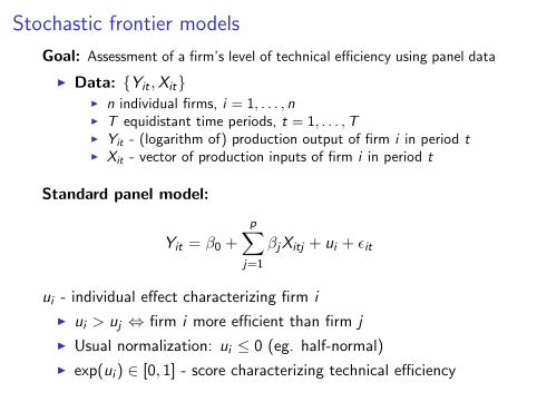
Stochastic frontier models

Goal: Assessment of a firm’s level of technical efficiency using panel data

I Data: {Yit ,Xit}I n individual firms, i = 1, . . . , nI T equidistant time periods, t = 1, . . . ,TI Yit - (logarithm of) production output of firm i in period tI Xit - vector of production inputs of firm i in period t

Standard panel model:

Yit = β0 +

p∑j=1

βjXitj + ui + ϵit

ui - individual effect characterizing firm i

I ui > uj ⇔ firm i more efficient than firm j

I Usual normalization: ui ≤ 0 (eg. half-normal)

I exp(ui ) ∈ [0, 1] - score characterizing technical efficiency

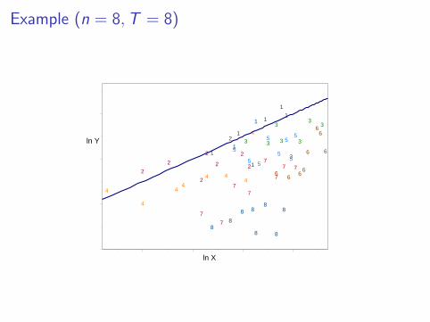
Example (n = 8,T = 8)

11

1

1

1 1

1

1

2

2

2

2

2

2

2

2

3 3

3

3

3

3

33

4

4

44

4 44

4

5

5 5

5

5

5

5

5

66

66

6

66

6

7

7

77

7

7

7 7

88

8 8

8

8

8

8

ln X

ln Y

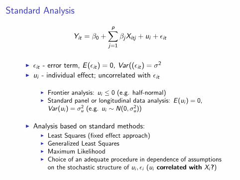
Standard Analysis

Yit = β0 +

p∑j=1

βjXitj + ui + ϵit

I ϵit - error term, E (ϵit) = 0, Var((ϵit) = σ2

I ui - individual effect; uncorrelated with ϵit

I Frontier analysis: ui ≤ 0 (e.g. half-normal)I Standard panel or longitudinal data analysis: E (ui ) = 0,

Var(ui ) = σ2u (e.g. ui ∼ N(0, σ2

u))

I Analysis based on standard methods:I Least Squares (fixed effect approach)I Generalized Least SquaresI Maximum LikelihoodI Choice of an adequate procedure in dependence of assumptions

on the stochastic structure of ui , ϵi (ui correlated with Xi?)

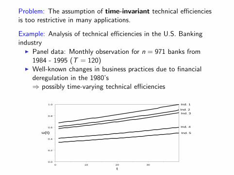
Problem: The assumption of time-invariant technical efficienciesis too restrictive in many applications.

Example: Analysis of technical efficiencies in the U.S. Bankingindustry

I Panel data: Monthly observation for n = 971 banks from1984 - 1995 (T = 120)

I Well-known changes in business practices due to financialderegulation in the 1980’s⇒ possibly time-varying technical efficiencies

0 10 20 30

t

0.0

0.2

0.4

0.6

0.8

1.0

u(t)

Ind. 1

Ind. 2Ind. 3

Ind. 4

Ind. 5

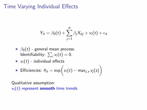
Time Varying Individual Effects

Yit = β0(t) +

p∑j=1

βjXitj + vi (t) + ϵit

I β0(t) - general mean process.Identifiability:

∑i vi (t) = 0.

I vi (t) - individual effects

I Efficiencies: θit = exp

(vi (t)−maxj ,s vj(s)

)Qualitative assumption:vi (t) represent smooth time trends

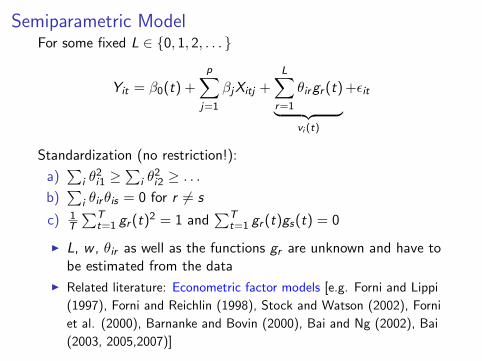
Semiparametric ModelFor some fixed L ∈ {0, 1, 2, . . . }

Yit = β0(t) +

p∑j=1

βjXitj +L∑

r=1

θirgr (t)︸ ︷︷ ︸vi (t)

+ϵit

Standardization (no restriction!):

a)∑

i θ2i1 ≥

∑i θ

2i2 ≥ . . .

b)∑

i θirθis = 0 for r = s

c) 1T

∑Tt=1 gr (t)

2 = 1 and∑T

t=1 gr (t)gs(t) = 0

I L, w , θir as well as the functions gr are unknown and have tobe estimated from the data

I Related literature: Econometric factor models [e.g. Forni and Lippi

(1997), Forni and Reichlin (1998), Stock and Watson (2002), Forni

et al. (2000), Barnanke and Bovin (2000), Bai and Ng (2002), Bai

(2003, 2005,2007)]

ExamplesExample with L = 3 (Cornwell, Schmidt and Sickles (1990)):

Yit = β0 +

p∑j=1

βjXitj + θi0 + θi1t + θi2t2︸ ︷︷ ︸

vi (t)

+ϵit

Example with L = 1 (Battese and Coelli (1992)):

Yit = β0 +

p∑j=1

βjXitj + θi exp(η(t − T ))︸ ︷︷ ︸vi (t)

+ϵit

Example with L = 1: Random walk

Yit = β0 +

p∑j=1

βjXitj + θig(t)︸ ︷︷ ︸vi (t)

+ϵit , g(t + 1) = g(t) + δt ,

for i.i.d. innovations δ1, δ2, . . .with E(δt) = 0, var(δt) = σ2δ .

Identifiability

Model: Yit = β0(t) +∑p

j=1 βjXitj +∑L

r=1 θirgr (t) + ϵit

Identifiability of the model requires that all variables Xitj possess aconsiderable variation over t = 1, . . . ,T . Effects of time-invariantsocioeconomic or demographic variables are captured by thecoefficients θir

Example: Standard panel model with p time-changing and qtime-invariant variables, Xitj ≡ Xij , j = p + 1, . . . , p + q.⇒ The models holds with L = 1 and g1(t) ≡ 1,

Yit = β0 +

p∑j=1

βjXitj +

p+q∑j=p+1

βjXij + ui︸ ︷︷ ︸θi1

+ϵit

I Regression of θi1 on Xi ,p+1, . . . ,Xi ,p+q ⇒ βp+1, . . . , βp+q

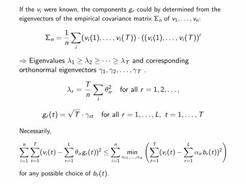
If the vi were known, the components gr could by determined from the

eigenvectors of the empirical covariance matrix Σn of v1, . . . , vn:

Σn =1

n

∑i

(vi (1), . . . , vi (T )) · ((vi (1), . . . , vi (T ))′

⇒ Eigenvalues λ1 ≥ λ2 ≥ · · · ≥ λT and correspondingorthonormal eigenvectors γ1, γ2, . . . , γT .

λr =T

n

∑i

θ2ir for all r = 1, 2, . . . ,

gr (t) =√T · γrt for all r = 1, . . . , L, t = 1, . . . ,T

Necessarily,

n∑i=1

T∑t=1

(vi (t)−L∑

r=1

θirgr (t))2 ≤

n∑i=1

minαi1,...,αiL

(T∑t=1

(vi (t)−L∑

r=1

αirbr (t))2

)

for any possible choice of br (t).

EstimationRecall: Yit = β0(t) +

∑pj=1 βjXitj + vi (t)︸︷︷︸∑L

r=1 θirgr (t)

+ϵit

Step 1. Semi-parametric estimation of β and vi (partial leastsquares):

Determine β1, . . . , βp and functional approximations νi (t) byminimizing

∑i

1

T

∑t

(Yit − Yt −p∑

j=1

βj(Xitj − Xtj)− νi (t))2

+ κ∑i

1

T

∫ T

1

(ν(m)i (s))2ds

Then estimate vi (t) by vi (t) := νi (t), t = 1, . . . ,T , i = 1, . . . , n.

I κ - smoothing parameter

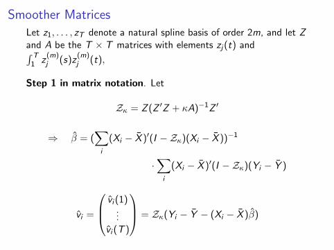
Smoother Matrices

Let z1, . . . , zT denote a natural spline basis of order 2m, and let Zand A be the T × T matrices with elements zj(t) and∫ T1 z

(m)j (s)z

(m)j (t),

Step 1 in matrix notation. Let

Zκ = Z (Z ′Z + κA)−1Z ′

⇒ β = (∑i

(Xi − X )′(I −Zκ)(Xi − X ))−1

·∑i

(Xi − X )′(I −Zκ)(Yi − Y )

vi =

vi (1)...

vi (T )

= Zκ(Yi − Y − (Xi − X )β)

Step 2: Estimate the empirical covariance matrix by

Σn =1

n

∑i

vi v′i

and calculate its

I eigenvalues λ1 ≥ λ2 ≥ . . . λT

I eigenvectors γ1, γ2, . . . , γT

Step 2: Setgr (t) =

√T · γrt

For i = 1, . . . , n determine θ1i , . . . , θLi by minimizing

∑t

(Yit − Yt −p∑

j=1

βj(Xitj − Xtj)−L∑

r=1

θri gr (t))2

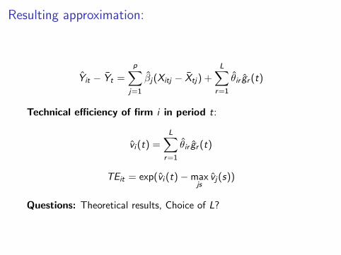
Resulting approximation:

Yit − Yt =

p∑j=1

βj(Xitj − Xtj) +L∑

r=1

θir gr (t)

Technical efficiency of firm i in period t:

vi (t) =L∑

r=1

θir gr (t)

TEit = exp(vi (t)−maxjs

vj(s))

Questions: Theoretical results, Choice of L?

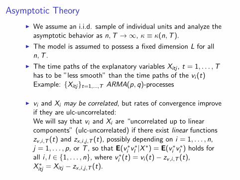
Asymptotic Theory

I We assume an i.i.d. sample of individual units and analyze theasymptotic behavior as n,T → ∞, κ ≡ κ(n,T ).

I The model is assumed to possess a fixed dimension L for alln,T .

I The time paths of the explanatory variables Xitj , t = 1, . . . ,Thas to be ”less smooth” than the time paths of the vi (t)Example: {Xitj}t=1,...,T ARMA(p, q)-processes

I vi and Xi may be correlated, but rates of convergence improveif they are ulc-uncorrelated:We will say that vi and Xi are “uncorrelated up to linearcomponents” (ulc-uncorrelated) if there exist linear functionszv ,i ,T (t) and zx ,i ,j ,T (t), possibly depending on i = 1, . . . , n,j = 1, . . . , p, or T , so that E(v∗i v

∗l |X ∗) = E(v∗i v

∗l ) holds for

all i , l ∈ {1, . . . , n}, where v∗i (t) = vi (t)− zv ,i ,T (t),X ∗itj = Xitj − zx ,i ,j ,T (t).

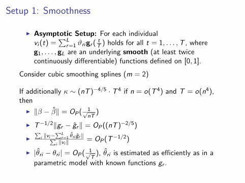
Setup 1: Smoothness

I Asymptotic Setup: For each individualvi (t) =

∑Lr=1 ϑrigr (

tT ) holds for all t = 1, . . . ,T , where

g1, . . . , gL are an underlying smooth (at least twicecontinuously differentiable) functions defined on [0, 1].

Consider cubic smoothing splines (m = 2)

If additionally κ ∼ (nT )−4/5 · T 4 if n = o(T 4) and T = o(n4),then

I ∥β − β∥ = OP(1√nT

)

I T−1/2∥gr − gr∥ = OP((nT )−2/5)

I∑

i ∥vi−∑L

r=1 θri gr∥∑i ∥vi∥

= OP(T−1/2)

I |θri − θri | = OP(1√T), θri is estimated as efficiently as in a

parametric model with known functions gr .

Setup 2: Stochastic Trends

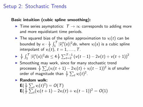
Basic intuition (cubic spline smoothing):

I Time series asymptotics: T → ∞ corresponds to adding moreand more equidistant time periods.

I The squared bias of the spline approximation to vi (t) can be

bounded by κ · 1T

∫ T1 |v ′′i (s)|2ds, where vi (s) is a cubic spline

interpolant of vi (t), t = 1, . . . ,T .

I 1T

∫ T1 |v ′′i (s)|2ds ≤ 4 1

T

∑T−1t=2 (v(t − 1)− 2v(t) + v(t + 1))2

I Smoothing may work, since for many stochastic trendprocesses 1

T

∑t(vi (t + 1)− 2vi (t) + vi (t − 1))2 is of smaller

order of magnitude than 1T

∑t vi (t)

2.

I Random walk:E( 1

T

∑t vi (t)

2) = O(T )E( 1

T

∑t(vi (t + 1)− 2vi (t) + vi (t − 1))2 = O(1)

Example: Independent random walksLet

vi (t) :=L∑

r=1

ϑrigr (t), with gr (t + 1) = gr (t) + δr ,t ,

δr ,1, δr ,2, . . . i.i.d, E (δr ,t) = 0, var(δr ,t) = σ2δ,t .

If κ ∼ (nT )−1/2, then

I

∥β − β∥ =

OP(

1√nT

) if Xi and vi are ulc-uncorrelated

OP(1√T) else

I T−1/2∥gr − gr∥ = OP(T−3/2 + (nT )−1/2)

I∑

i ∥vi−∑L

r=1 θri gr∥∑i ∥vi∥

= OP(T−3/2 + (nT )−1/2)

I |θri − θri | = OP(1√T)

General theoretical results

Note:

I Smoothness asymptotics: vi (t) = νi (tT )

⇒ 1T

∑t vi (t)

2 →∫ 10 νi (t)

2dt as T → ∞I Stochastic trends: usually 1

T

∑t vi (t)

2 → ∞ as T → ∞

Theoretical results depend on c(T ), b(T ), and d(T ) whichquantify the rate of increase of 1

T

∑t vi (t)

2, of the correspondingsecond order differences, and of

∑X 2itj :

I E( 1T

∑Tt=1 vi (t)

2) =: c(T )

I E(

1T

∑T−1t=2 (vi (t − 1)− 2vi (t) + vi (t + 1))2

)=: b(T )

I E( 1T

∑Tt=1 X

2it,j) =: d(T )

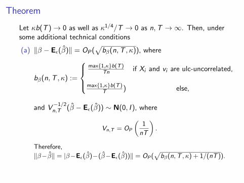
Theorem

Let κb(T ) → 0 as well as κ1/4/T → 0 as n,T → ∞. Then, undersome additional technical conditions

(a) ∥β − Eϵ(β)∥ = OP(√

bβ(n,T , κ)), where

bβ(n,T , κ) :=

max{1,κ}b(T )

Tn if Xi and vi are ulc-uncorrelated,

max{1,κ}b(T )T ) else,

and V−1/2n,T (β − Eϵ(β)) ∼ N(0, I ), where

Vn,T = OP

(1

nT

).

Therefore,

∥β−β∥ = |β−Eϵ(β)−(β−Eϵ(β))∥ = OP(√

bβ(n,T , κ) + 1/(nT )).

(b) For all r = 1, . . . , L

T−1/2∥gr−gr∥ = OP

(√κb(T ) + d(T )bβ(n,T , κ)

c(T )+

1

nc(T )max{1, κ1/4}

),

where κ = min{κ, κ2}.

(c) For all r = 1, . . . , L

|θri−θri | = OP

(√T−1 + κb(T ) + d(T )bβ(n,T , κ) + (nmax{1, κ1/4})−1

).

Furthermore, ifκb(T ) + d(T )bβ(n,T , κ) + (nmax{1, κ1/4})−1 = o(T−1),then √

T (θ1i − θ1i , . . . , θLi − θLi )′ →d N(0, σ2I ).

(d) For all i = 1, . . . , n∑i ∥vi −

∑Lr=1 θri gr∥∑

i ∥vi∥

= OP

(√T−1 + κb(T ) + d(T )bβ(n,T , κ) + (nmax{1, κ1/4})−1

c(T )

).

(e) If additionally Tnmax{1,κ1/4} → 0 as well as

Td(T )bβ(n,T , κ) + d(T )n + 1

Tc(T ) = o(

Tnmax{1,κ1/4}

), then

n∑T

r=L+1 λr − (n − 1)σ2 · tr(ZκPLZκ)

σ2

√2n · tr((ZκPLZκ)2)

→d N(0, 1),

n · tr(PLΣn,T )− (n − 1)σ2 · tr(ZκPLZκ)

σ2√2n · tr((ZκPLZκ)2)

→d N(0, 1),

where PL = I − 1T

∑Lr=1 gr g

′r , and PL is the projection matrix

projecting into the n − L dimensional linear space orthogonal to

span{Zκg1, . . . ,ZκgL}.

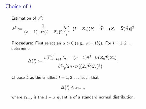
Choice of L

Estimation of σ2:

σ2 :=1

(n − 1) · tr(I −Zκ)2

∑i

∥(I −Zκ)(Yi − Y − (Xi − X )β)∥2

Procedure: First select an α > 0 (e.g., α = 1%). For l = 1, 2, . . .determine

∆(l) :=n∑T

r=l+1 λr − (n − 1)σ2 · tr(ZκPlZκ)

σ2

√2n · tr((ZκPlZκ)2)

.

Choose L as the smallest l = 1, 2, . . . such that

∆(l) ≤ z1−α,

where z1−α is the 1− α quantile of a standard normal distribution.

Choice of κ

A smoothing parameter κ may be chosen by cross-validation:

CV (κ) :=1

nT

∑i

∑t

(Yit − Yt − (Xit − Xt)β−i −L∑

r=1

θr ,−i gr ,−i (t))2

I β−i , gr ,−i - estimates of β and gr obtained from the data(Ykj ,Xkj), k = 1, . . . , i − 1, i + 1, . . . , n, j = 1, . . . ,T

I θr ,−i - corresponding estimates of θri to be obtained when

using β−i , gr ,−i instead of β, gr

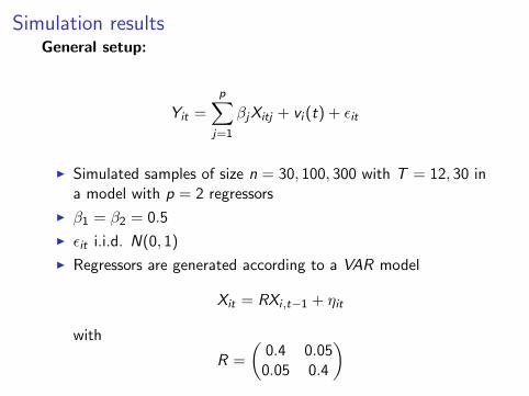
Simulation resultsGeneral setup:

Yit =

p∑j=1

βjXitj + vi (t) + ϵit

I Simulated samples of size n = 30, 100, 300 with T = 12, 30 ina model with p = 2 regressors

I β1 = β2 = 0.5

I ϵit i.i.d. N(0, 1)

I Regressors are generated according to a VAR model

Xit = RXi ,t−1 + ηit

with

R =

(0.4 0.050.05 0.4

)

Monte Carlo Simulation Results for DGP1:

vi (t) = θi0 + θi1t

T+ θi2

( t

T

)2MSE of Coefficients

N T Within GLS CSSW KSS

30 12 0.07258 0.06381 0.00867 0.0087430 0.02832 0.02355 0.00240 0.00258

100 12 0.01862 0.01643 0.00266 0.0027330 0.00678 0.00649 0.00073 0.00075

300 12 0.00610 0.00609 0.00086 0.0008730 0.00210 0.00208 0.00023 0.00023

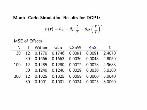
Monte Carlo Simulation Results for DGP1:

vi (t) = θi0 + θi1t

T+ θi2

( t

T

)2MSE of Effects

N T Within GLS CSSW KSS L

30 12 0.1770 0.1746 0.0091 0.0091 2.407030 0.1666 0.1663 0.0036 0.0043 2.8050

100 12 0.1285 0.1280 0.0072 0.0073 2.968830 0.1240 0.1240 0.0029 0.0030 3.0100

300 12 0.1025 0.1025 0.0059 0.0060 3.004030 0.1001 0.1001 0.0024 0.0025 3.0060

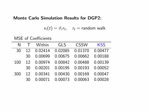
Monte Carlo Simulation Results for DGP2:

vi (t) = ϑi rt , rt = random walk

MSE of Coefficients

N T Within GLS CSSW KSS

30 12 0.02414 0.02085 0.01370 0.0047730 0.00699 0.00675 0.00662 0.00188

100 12 0.00974 0.00842 0.00488 0.0013930 0.00201 0.00195 0.00193 0.00052

300 12 0.00341 0.00430 0.00169 0.0004730 0.00071 0.00073 0.00063 0.00028

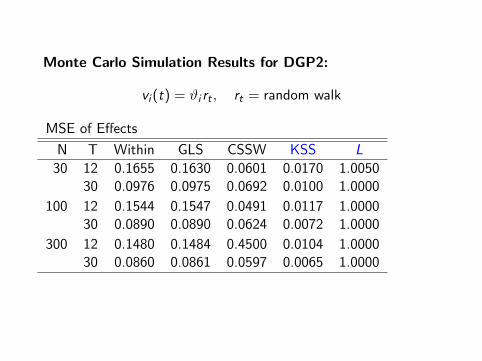
Monte Carlo Simulation Results for DGP2:

vi (t) = ϑi rt , rt = random walk

MSE of Effects

N T Within GLS CSSW KSS L

30 12 0.1655 0.1630 0.0601 0.0170 1.005030 0.0976 0.0975 0.0692 0.0100 1.0000

100 12 0.1544 0.1547 0.0491 0.0117 1.000030 0.0890 0.0890 0.0624 0.0072 1.0000

300 12 0.1480 0.1484 0.4500 0.0104 1.000030 0.0860 0.0861 0.0597 0.0065 1.0000

Monte Carlo Simulation Results for DGP4:

vi (t) ≡ ϑi standard panel model

MSE of Coefficients

N T Within GLS CSSW KSS

30 12 0.00544 0.00484 0.00841 0.0061530 0.00188 0.00181 0.00221 0.00200

100 12 0.00176 0.00122 0.00262 0.0018330 0.00061 0.00051 0.00073 0.00062

300 12 0.00056 0.00080 0.00086 0.0005830 0.00020 0.00026 0.00024 0.00020

Monte Carlo Simulation Results for DGP4:

vi (t) ≡ ϑi standard panel model

MSE of Effects

N T Within GLS CSSW KSS L

30 12 0.1213 0.1126 0.3387 0.1519 1.032030 0.0472 0.0462 0.1288 0.0638 1.0100

100 12 0.0929 0.0876 0.2706 0.1032 1.043030 0.0363 0.0354 0.1062 0.0414 1.0230

300 12 0.0795 0.0811 0.2366 0.0838 1.028030 0.0319 0.0323 0.0947 0.0339 1.0200

Monte Carlo Simulation Results for DGP5 (L = 6):

vi (t) = 3(ϑi0 + ϑi1t

T+ θi2

( t

T

)2) + ϑi3rt + ϑi4g1t + ϑi5g2t

with rt+1 = rt + δt , g1t = sin(πt/4), g2t = cos(πt/4).

MSE of Coefficients

N T Within GLS CSSW KSS

30 12 13.3517 12.4807 5.3708 0.249530 4.3252 4.2655 1.5867 0.0141

100 12 3.863 3.3662 1.6696 0.034230 1.3015 1.2465 0.5392 0.0021

300 12 1.3521 1.1517 0.6465 0.006530 0.4562 0.4314 0.185 0.0009

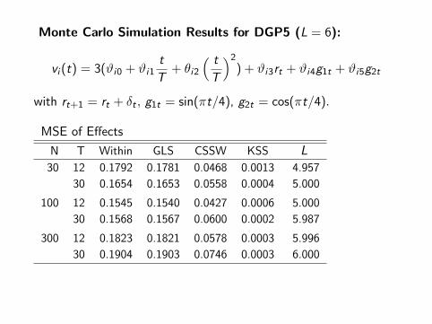
Monte Carlo Simulation Results for DGP5 (L = 6):

vi (t) = 3(ϑi0 + ϑi1t

T+ θi2

( t

T

)2) + ϑi3rt + ϑi4g1t + ϑi5g2t

with rt+1 = rt + δt , g1t = sin(πt/4), g2t = cos(πt/4).

MSE of Effects

N T Within GLS CSSW KSS L

30 12 0.1792 0.1781 0.0468 0.0013 4.957

30 0.1654 0.1653 0.0558 0.0004 5.000

100 12 0.1545 0.1540 0.0427 0.0006 5.000

30 0.1568 0.1567 0.0600 0.0002 5.987

300 12 0.1823 0.1821 0.0578 0.0003 5.996

30 0.1904 0.1903 0.0746 0.0003 6.000

ApplicationAnalysis of technical efficiencies in the U.S. Banking industry

I Panel data: Monthly observation for n = 971 banks from1984 - 1995 (T = 120)

I Well-known changes in business practices due to financialderegulation in the 1980’s⇒ possibly time-varying technical efficiencies

I Estimated dimension of the model L = 7

1 2 3 4 5 6 7 8 9 10 11 120.55

0.56

0.57

0.58

0.59

0.6

0.61

0.62

0.63

0.64

0.65

Time

Effic

iency

CSSWKSSBC