Modern Economy, 2011, 2, 203-212 doi:10.4236/me.2011.23026 Published Online July 2011 (http://www.SciRP.org/journal/me)

Copyright © 2011 SciRes. ME

A New Model for AS-AD Analysis Based on Input-Output Frame

Xinjian Liu School of Economics and Management, Yanshan University, Qinhuangdao, China

E-mail: lxj6309@126.com, lxj@ysu.edu.cn Received February 11, 2011; revised March 29, 2011; accepted April 18, 2011

Abstract This paper has established a new kind of AS-AD models with input-output techniques. The models take the standard input-output tables as its starting points. We analyze the change effects of government consumption, direct consumption coefficient, labor productivity, and surplus rate on the equilibrium output. In this paper, we propose that the aggregate demand function curve should be right upward, and this lead to a series of in-consistent conclusions with the traditional views. Finally, we also analyze the well-known issue of stagfla-tion. Keywords: AS-AD Model, Input-Output, Aggregate Supply, Aggregate Demand

1. Introduction

It was pointed out that the input-output (IO) analysis had no longer been included in the core of mainstream eco-nomics since the middle of 1980s. The authoritative magazines, such as Econometrica, the Review of Eco-nomics and Statistics, and the Quarterly Journal of Eco-nomics, didn’t continue to publish input-output papers, and the best economists seemed seldom to have interest in the development of input-output analysis field [1]. In fact, input-output (IO) economics has never had access to the core of mainstream economics. Leontief’s input- output economics[2] and Keynesian economics[3] were both generated in the mid-1930s, but the Keynesian the-ory is the inheritance and development of traditional mainstream economics and has the same basic category to it, whereas the Leontief theory born out of Marxist economics and is completely different from the tradi-tional classic economics in the core category. The key difference between them is that the foundation concept of Keynesian theory is national income such as GNP or GDP, and the foundation concept of Leontief theory is total output which contains intermediate inputs, such that the Keynesian theory’s research object mainly focused on the transaction processes and the Leontief theory’s object mainly focused on the production processes. Although IO analysis has obtained a huge developing space in the study of practical economies, it is yet impossible to enter the mainstream economic theory system. They two can

not be combined together seamlessly. However, Leontief’s theory is closer to reality than the mainstream one be-cause some intermediate inputs are necessary for most of real production processes and any unit of products must contain some products which were produced previously. The AS-AD analysis approach is a new development stage of the mainstream economics in the 1980s to 1990s when it was used to solve the stagflation problems which had troubled mainstream economics for more than 20 years.

This paper develops a new AS-AD model with a sin-gle-sector IO framework and analyses the slopes of new AD and AS functions at first, and then explores the im-pacts of government expenditure, direct consumption coefficient, labor productivity and operating surplus rate on the equilibrium states in the second part. It discusses the stagflation issue in a two-sector model in the third part. The last part gives the conclusion views of the paper

2. Single-Sector AS-AD Model

2.1. Basic Input-Output Relations

The model of a single-sector input-output table shown as following:

1 2

X C G I NX

W

T T

Z

X. J. LIU

Copyright © 2011 SciRes. ME

204

where X is intermediate input (or intermediate use), C is household consumption, G is public consumption(or government consumption), I is capital formation, NX is net export, W is total wage, 1T is net taxes on produc-tion, 2T is net taxes on income, Z is operating surplus.

For this economic system, its input-output balance re-lations are following:

X C G I NX Q (1)

1PX W T Z PQ (2)

where P is the price level, Q is the total output. If let dQ denote aggregate demand and sQ denote

aggregate supply, then Formulas (1) and (2) should be written as following:

dX C G I NX Q (3)

1sPX W T Z PQ (4)

When the supply and demand are balanced, there is d sQ Q

Formulas (3) and (4) show that the rows of an IO table represent the demand sides of an economy and the col-umns represent the production processes.

2.2. Aggregate Demand (AD) Relations

If we have the behavioral functions of the aggregate de-mand as following:

sX Q a , 1 ,C f W Z P , 1 2G T T H ,

2 ,I f r Z P , 3 ,dNX f Q e ,

where a is the direct consumption coefficient, H is a planned deficit, r is an interest rate, e is an exchange rate.

The above behavioral functions contain following ba-sic ideas:

1) In a short term, a is constant. This is not only the basic usage of input-output techniques, but also con-forms to the characteristics of short-term economy.

2) For a given economic system, consumption was mainly influenced by income. The resident income in-cludes two main parts: one is the total wage which con-sidered as remuneration for labor, and the other is from operating surplus which considered usually as capital income. For a national economy, income also includes the transfer payments (ignored here) from abroad. The influences on consumption from wage W or surplus Z are very different. Z’s main function is to provide the in-vestment fund for expanded reproduction; W’s main function is to provide consumption fund.

3) A large part of the government expenditure is a short-term or annual decision variable, so financial defi-

cit, for a functional finance, may be a short-term deci-sion-making. Generally, taxation as a long-term factor cannot change greatly and frequently. The deficit deci-sion-making which generally takes GDP as a benchmark is a percentage of GDP and can not be too large.

4) As derived demand, investment is not only affected by financial interest rate r , but also affected by surplus level. Obviously, the higher the surplus level is, the big-ger the power of enterprises investment is. In this paper we will not discuss the balanced problem of money market, but directly take r as a kind of exogenous con-stant. We do not consider its change in the following analysis, so it will be omitted in the investment function. Although the bank deposit and loan interest rates may be endogenous as market variables in microeconomic level, the modern economic system provides a space for mone-tary policy. The guidance or benchmark interest rate is drawn up by the central department of financial man-agement. The real interest rate fluctuates generally above or below the guidance interest rate. From the macro-scopic effect, the benchmark interest rate affects the level of investment through control rules.

5) What affects the economic import and export level is not only exchange rate, but also the economic level of activity as a major contributing factor for import and export in fact. This factor can be represented by demand level. The changes of imports and exports induced by aggregate supply can be embedded in X and I . This paper takes exchange rate as an exogenous constant and does not consider its change, so it will be omitted in the following analysis.

Substituting the above demand behavior functions into Formula (3), we will have

1 2 3,d s dQ Q a f W Z P f Z P f Q G (5)

where it is assumed that

1 1 1 1

2 2 33

0, 0,

0,1 0d

W Z

dZ Q

f f W f f Z

f f Z f f Q

When the price level is given constant and let s dQ Q , Formula (3) coupled with various behavior

functions can be equivalent to the IS formula in main-stream economics.

2.3. Aggregate Supply (AS) Relations

The main development of contemporary mainstream economics is about aggregate supply theory, and various schools’ arguments are mainly on the aggregate supply model. The traditional Keynes theory considers aggre-gate supply completely elastic in short term and thinks an economic equilibrium is mainly decided by aggregate demand. Neoclassic economics assumes that aggregate

X. J. LIU

Copyright © 2011 SciRes. ME

205

supply is decided by the people’s expectation of price level. If the expectation is rational, the expected price will be consistent with the actual price. Thus, the aggre-gate supply is equal to the natural rate of output and completely inelastic and is not disturbed by random fac-tors and macroeconomic policies. The new Keynesian economics believes that the market is not always cleared up because of the stickiness of wage and price, thus

eP P . Therefore, the aggregate supply is elastic, but is not completely elastic as Keynes defined. In the litera-tures of mainstream economics, there are many ways to define an aggregate supply function. In the following, we adopt the way used by Blanchard [4].

2.3.1. AS Function Derivation Steps of Blanchard Let’s first show how Blanchard derived AS function.

1) Wage decision function. Assuming

,ew P F u z (6)

where w is a wage rate, eP is an expected price level, u is an unemployment rate. This relation is decided by the supply and demand of labor together. For labors, if w rises and eP does not change, the supplied labor will increase and then u will decrease. For enterprises, the wages that they’re willing to pay when u rises will be reduced and the strength of wage bargaining of workers

will be weaken; thus 0u

FF

u

.

Formula (6) reflects the behavior characteristics when labor and capital bargain for employment contract. z represents the other factors which affect wage besides u and eP , such as the unemployment insurance level, the economic structure regulation and so on. Generally we assume z changes in the same direction with w . Formula (6) also means that what the labor and capital think highly of when they negotiate a labor contract is real wage( ew P )rather than nominal wage ( w ).

2) Production function. Assuming a simple produc-tion function:

Y AN

where N is the employed labor. If measuring the total output (National income) Y by a suitable unit which make 1A , thus

Y N (7)

then 1 1N Y

uL L

. Here L is the total labor force.

3) Price decision rule. Assuming

1P w (8)

where is called price markup. Formula (8) may re-gard as a cost-plus pricing model. The mainstream eco-nomics does not consider intermediate inputs, so the only

cost is wage at present. Blanchard pointed out that If the market is competitive completely, there are 0 , P w . Therefore, it considers a state of incomplete competition here.

4) Combination. Substitute Formula (6) into Formula (8), we get

1 ,eP P F u z (9)

5) Aggregate supply function. From the above formu-las, we may obtain the relation of P andY :

1 1 ,e YP P F z

L

(10)

2.3.2. AS Function in Input-Output System Similarly to Blanchard’s steps, we can establish the AS relation under an input-output framework. From Formula (4), we have 1

s s sPQ a wQ l T Z PQ where l is the labor input used to produce one unit product. Assuming that all labors are homogeneous and the work condition is the same, then l may be regarded as the labor num-ber taken by one unit product and w is the remuneration for one unit labor in certain time, so that sl N Q . Suppose that taxation is a proportion t of added value or GDP, then

1 1sT t wQ l T Z (11)

Similarly to Blanchard’s price deciding model, we as-sume that

sZ PQ (12)

From Formulas (11) and (12), we have

1 1 1

ss st tQ

T wQ l PQ wl Pt t

Let 11

tt

t

, then

1s s s s sPQ a wQ l t Q wl P PQ PQ

and then

1Pa wl t wl P P P

1

1

1

1 1

t wlP

a t

Let

10

1

1

1 1

tk

a t

, then it gets

0 0, 0P k wl k (13)

Formula (13) is just the price deciding formula in an input-output system. Then we apply Blanchard’s wage deciding relation i.e. Formula (6), there is

X. J. LIU

Copyright © 2011 SciRes. ME

206

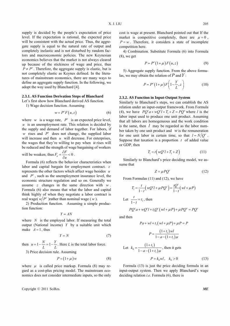
0 ,eP k lP F u z (14)

Introducing the production function sQ N l , then

1 1 sN lu Q

L L

Therefore we may have the AS function as following,

0 1 ,e slP k lP F Q z

L

(15)

We will not consider about the change effect of z, so that z will be omitted in the following context.

2.4. The Slope Signs of AD and AS Curves

For brief, we use the symbol 1 euwl u lP F ,

01 euP u k lP F .

2.4.1. AS Curve From Formulas (14) and (15), we have

0

0

d

d

d 1or

d

eus

s

eu

P lk lP F

LQ

Q L

P lk lP F

(16)

where uF express the partial derivative of function F to u1 the same below).

Because 0 0, 0uk F , so d

0d

sQ

P , thus the AS

curve inclines up toward right in the sP Q or sQ P space (see Figures 1-3 below).

2.4.2. AD Curve From Formula (5), we have

1 21

1 223

d d d d

d d d d

d

dd

d sZ ZW

d

Q

f ffQ Q W Za

P P P P P P

f fQf

P P

d d

d d

sW Q

P P

0

d d

d d (1 )

ss s

eu

Z Q ZP Q Q

P P u k lP F

From the above formulas, we may educe

1 21

3

1 2 1 22

d d1

d dd

d sZ ZW

Q

Z Z

f ffQ Qf a P

P P P P

f f Z f f

P

(17)

AS Q

AD′

E

P

E

AD

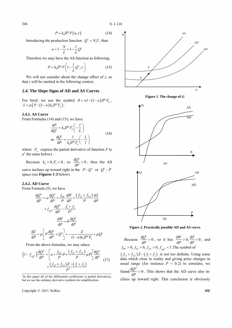
Figure 1. The change of G.

AS

AD

(a)

Q

P

AD

ASQ

P

(b)

Figure 2. Practically possible AD and AS curve.

Because d

0d

sQ

P , so it has

d d0, 0

d d

W Z

P P , and

1 1 2 30, 0, 0, 1dW Z Z Q

f f f f .The symbol of

1 2 1 2Z Zf f Z f f is not too definite. Using some data which close to reality and giving price changes in usual range (for instance P < 0.2) to simulate, we

foundd

0d

dQ

P . This shows that the AD curve also in-

clines up toward right. This conclusion is obviously 1In this paper all of the differential coefficients is partial derivatives, but we use the ordinary derivative symbols for simplification.

X. J. LIU

Copyright © 2011 SciRes. ME

207

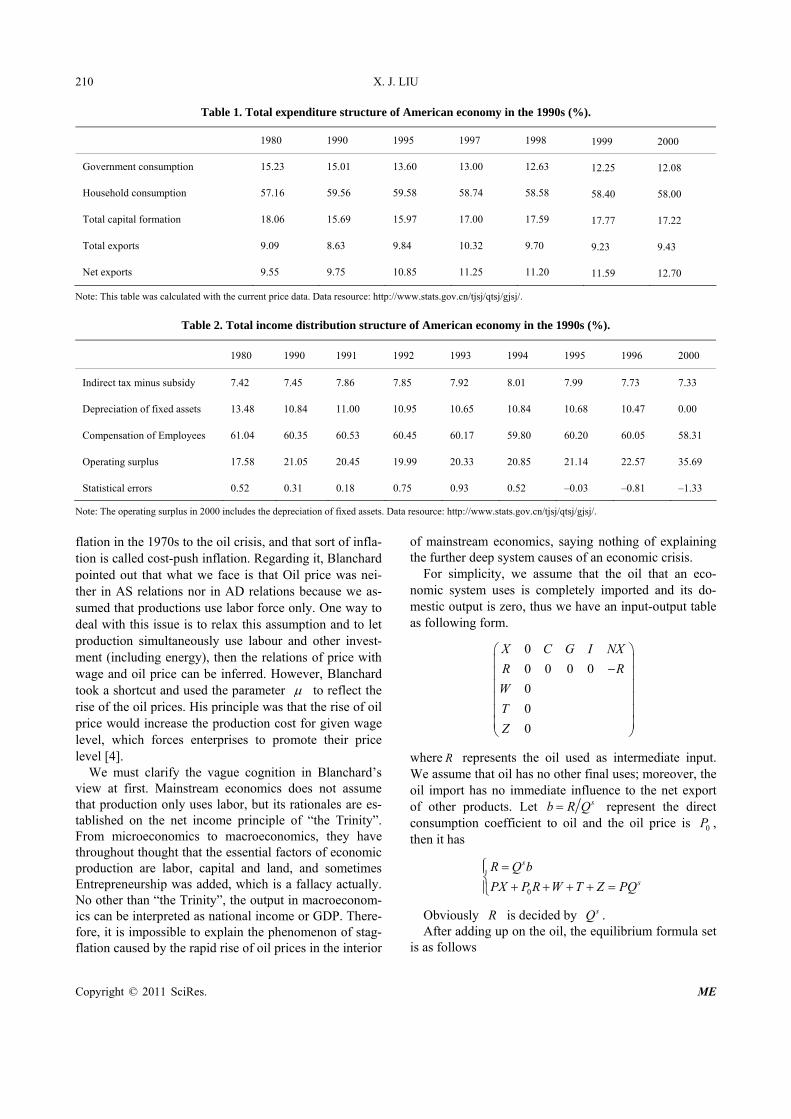
AS Q

AD′

AD

E

AS′

E′

P

Figure 3. The change of a. against the traditional theory. Let us see how this hap-pens.

In mainstream economics, the general derivation process of AD function starts with

ddY C Y G I r (for a closed economy)

where dY is disposable income, r is the interest rate

decided by money market. In money market, d

0d

r

P .

Because d d

d d

I rI r

P P , dd

d dd

d

YCC Y

P P ,and usually

ddY Y T (T is tax) and G is considered constant, so

d d 1

d d 1

d

d

Y I

P P C Y

. Because 0 1dC Y , 0I r ,

so that d

0d

dY

P . In fact, there is a subjective mistake of

self-righteousness in the above process of the deduction2.

That is we consider ddY Y T by mistake. Because

income roots in production process, while the production process is decided by supply, so actually it should

be d d

d d

s

d

C YC Y

P P . Because

d0

d

sY

P , so

d0

d

C

P . Thus

the symbol of d d d

d d d

dY C I

P P P will be not definite. If we

assume that r is constant, and I is the increasing func-

tion of Z , obviously we have d

0d

dY

P . Such a conclu-

sion also shows the differences between macroeconom-ics and microeconomics. Besides very few commodities

(such as Giffen commodity), the demand curves in mi-croeconomics should incline down toward right (this is a conclusion under given income). But AD curves in mac-roeconomics generally should incline up toward right and have the same orientation with AS curves. Looking from the real economy observation, this point is intui-tively correct. In macroeconomic level, the rise of price level shows that economic tends to be prosperous, the income will be higher and the demand will also increase. The investment would increase when price level move up. One reason for that mistake in traditional macroeco-nomics is that it was forgotten that the income determi-nation theory was derived out under aggregate supply equal to aggregate demand when simple Keynesian in-come determination theory was turned into AS-AD analysis, i.e. it assumes s sY C Y I G in advance. It must return to d sY C Y I G when deducing AD function. The total income used in LM model for money market should be the Y when aggregate supply is equal to aggregate demand. A proper macroeconomic analysis framework should be the combination of AD formula, AS formula and the money market formula, and an equilibrium state can be solved from these three for-mulas, but it is not to add the money market (or general financial market) formula to income determination model at first. The foreign exchange and the international money market should be added in for an open economy. In this paper, we assume the two markets are exogenous, i.e. r and e are given.

2.5. The Perturbations of AD and AS

With the AS and AD functions given above, we will make some comparative static analysis based on the per-turbations caused by several parameters in the following.

Being equilibrium, Qd = Qs, therefore the above sys-tem satisfies the following equilibrium formula group:

1 23

, ,,

f W Z f r ZQ Qa f Q e G

P P (5)′

0P k lw (13)′

,ew P F u z (6)′

1u Ql L

Z PQ (12)′

W Qlw

2.5.1. Changes of Government Consumption (G) Differentiating the above formulas with respect to G, we have

2Samuelson reminds people not to commit three mistakes in the intro-duction of his ‘Economics’ [5]. They are post hoc fallacy, fallacy of composition and subjectivity. He said let us alert the assuming condi-tion our subjective interest didn’t express definitely.

X. J. LIU

Copyright © 2011 SciRes. ME

208

20

0

0

d d d

d d d

1 d

d

e eu u

eu

P lF k l P FP Q Qk l

G L G L G

u k lP F Q

Q G

(18)

1 1 2

1

01 232

d1

d

1

W Z Z

eu

Q

f f fQa

G P P

u k lP Ff ff

QP

(19)

Let

1 1 2

01 232

1

1

W Z Z

eu

Q

f f fB a

P P

u k lP Ff ff

QP

,

then 1d

d

QB

G .

Because the change of G has no influence on AS and it makes AD increase, thus it should also make the equilib-rium gross output increase, namely there should be d

0d

Q

G . Because 0uF , according to Formula (18),

there should be d

0d

P

G . Therefore, the expansion of

government consumption can make the equilibrium price and equilibrium output increase simultaneously. Thus, according to Formula (19), there should be

1 1 2

01 232

1

1 0

W Z Z

eu

Q

f f fB a

P P

u k lP Ff ff

QP

(20)

From the above results, we may also have

d d

d d

s dQ Q

P P at the equilibrium point, otherwise

d0

d

Q

G

and d

0d

P

G which is unreasonable. However, when an

economy is close to potential production, there will be

d0

d

sQ

P certainly and may have

d d

d d

s dQ Q

P P (See

Figure 1), thus d d

0 and 0d d

Q P

G G may appear. We

need introduce the money market and the foreign ex-change market to explain or solve this problem. In fact a serious bubble economy appears then and the income no longer originates from production but from speculation or the unusual inflow of foreign exchange. On the other hand, because the economy is close to potential produc-

tion, there should also be d

0d

dQ

P . Therefore, the pos-

sible AS and AD curves may be as that in Figure 2.

2.5.2. Changes of Direct Consumption Coefficient (a) Direct consumption coefficient is the characteristic pa-rameter of input-output analysis. By intuition, the in-crease of a will enhance the marginal cost, thus the price will rise, and equilibrium output reduces possibly. This conclusion is generally correct in microeconomics. We will observe the microeconomic effects with AS-AD model in an input-output system in the following.

Differentiating the equilibrium formulas with respect to a, we have:

00

0

1

dd d

d d

1 d

1 1 du

kP wl w k

Ea a a

eu lk P FP Q

a t Q a

(21)

1d d d

d d du

u

eu P Fw l Q QeP Fa L a Q a

(22)

1 2 1 212

1 1

d

d

1 1 1 1Z Z

Q

a

Z f f P f fB Q

P a t P a t

(23)

Obviously it isd

0d

Q

a . Substituting Formula (23) into

Formula (21), we might judge immediately that d

0d

P

a .

These results are opposite to the microeconomic situation. This may be explained as following. Though the increase of direct consumption coefficient increases the cost, it also enhances the demand simultaneously. From the

Formula about d

d

w

a, we know that the wage rate will

also enhance, thus the consumer demand will also en-hance and the investment demand will also increase. Therefore, the final results are that equilibrium output may also enhance simultaneously when the price rises. According to Formulas (16) and (17), the increase of a will make the slope of AS curve decrease and simulta-neously the slope of AD curve may increase or decrease (See Figure 3). If the reduction of AD curve slope is within a certain range, the equilibrium output still en-hances. If the slope of AD curve increases, the equilib-rium gross output must increase.

2.5.3. Changes of Labor Productivity If labor productivity increases (i.e. l reduces), an enter-

X. J. LIU

Copyright © 2011 SciRes. ME

209

prise’s marginal cost will reduce, thus it will cause the reduction of market price of that product and the increase of equilibrium output. Now let us see the macroeconomic situation.

Differentiating the equilibrium formulas with respect to l, we have

d d

d d

1 1

u

u u

w l Q QeP Fl L l L

e eu P F u P FdQ

Q dl l

(24)

0

0 0

d d

d d

d1 1

de

u

P wk w l

l l

l Qk w u k P F

Q l

(25)

10 0

1 2 1 2102

d1

de

u

Z ZW

QB k w u k P F

l

f f Z f ffQ k

P P

(26)

According to Formula (26), we can judge that d

0d

P

l

from Formula (25) so long as d

0d

Q

l . This means that

the increase of productivity (i.e. decrease of l) will re-duce output and price level. Why does this happen? The reason is that although the enhancement of labor produc-tivity increases the aggregate supply (this can be proven from Formula (15)), simultaneously it also causes the augment of unemployment rate3 and the decrease of wage rate further. These two kinds of changes will obvi-ously reduce the income, thus it causes the consumption demand reduced and makes the equilibrium aggregate output decrease finally. This conclusion seems to contra-dict with real situation. This paradox’s solution relies on the changes of international market. The increase of la-bor productivity would enhance export competitiveness and increase export demand obviously, which would influence investment demand in turn, and then equilib-rium output was finally augmented. However, the do-mestic consumption demand would not increase neces-sarily at the same time4. In the 1990s of the productivity increase and economic expansion caused by new econ-omy, for the Expenditure structure of US GDP from

1990 to 2000, the net import proportion increased 2.95 percentage points, the total capital formation increased 1.53 percentage points, the government consumption dropped 2.93 percentage points, and the household con-sumption reduced 1.56 percentage points. Looking into the structure of income distribution, the Compensation of Employees reduced 2.04 percentage points but the oper-ating surplus (including depreciation of fixed assets) in-creased 3.8 percentage points (See Tables 1 and 2 for details). Therefore, how to transform the benefits of productivity increase into the income of ordinary resi-dents and the increase of consumption level needs the support of government incomes policies (including tax policy), otherwise an economy would go to serious im-balance someday.

2.5.4. Changes of Operating Surplus Rate (μ) The enterprises’ strength would enhance in the labor market when operating surplus increase, which means they can extort more surpluses therefore the aggregate supply would increase. The changes of aggregate de-mand rely on whether the increase of income caused by supply increase may compensate the income reduction caused by the reduction of labour reward share.

Differentiating the equilibrium formulas with respect to μ, we will deduce

1d d d

d d d

ee

uu P Fw l Q Q

P FL Q

00 0

0 20

dd d d

d d d d

1 d

d

eu

kP wk wl l k w

u k P F Ql wk

Q

0 1 211 2 0

d1

d Z Z

k f fQB f f Q k

P

From the above, it has d

0d

Q

,

d0

d

P

. Therefore,

the increase of surplus proportion causes the equilibrium output to expand.

3. The Explanation of Stagflation Issues

The mainstream economics generally attributes the stag-

3In Formula (15), it is 0 1 ,le sP k lP F Q zL

= 0 ,ek lP F u z . Let P

= constant, then doing differentiation, thus d, 0

du

uF u z lF

l . Be-

cause 0,uF so thatd

0d

u

l .

4Jorgenson once found, ‘comparing the contribution of intermediate input with other source of output growth demonstrates that this input is by far the most significant source of growth. The contribution of inter-mediate input (for output increase) exceeds productivity growth and the contribution of capital and labor inputs. If we focus attention on the contribution of capital and labor inputs alone, excluding intermediate input from consideration, these two inputs are a more important source of growth than changes in productivity’ [6].

X. J. LIU

Copyright © 2011 SciRes. ME

210

Table 1. Total expenditure structure of American economy in the 1990s (%).

1980 1990 1995 1997 1998 1999 2000

Government consumption 15.23 15.01 13.60 13.00 12.63 12.25 12.08

Household consumption 57.16 59.56 59.58 58.74 58.58 58.40 58.00

Total capital formation 18.06 15.69 15.97 17.00 17.59 17.77 17.22

Total exports 9.09 8.63 9.84 10.32 9.70 9.23 9.43

Net exports 9.55 9.75 10.85 11.25 11.20 11.59 12.70

Note: This table was calculated with the current price data. Data resource: http://www.stats.gov.cn/tjsj/qtsj/gjsj/.

Table 2. Total income distribution structure of American economy in the 1990s (%).

1980 1990 1991 1992 1993 1994 1995 1996 2000

Indirect tax minus subsidy 7.42 7.45 7.86 7.85 7.92 8.01 7.99 7.73 7.33

Depreciation of fixed assets 13.48 10.84 11.00 10.95 10.65 10.84 10.68 10.47 0.00

Compensation of Employees 61.04 60.35 60.53 60.45 60.17 59.80 60.20 60.05 58.31

Operating surplus 17.58 21.05 20.45 19.99 20.33 20.85 21.14 22.57 35.69

Statistical errors 0.52 0.31 0.18 0.75 0.93 0.52 –0.03 –0.81 –1.33

Note: The operating surplus in 2000 includes the depreciation of fixed assets. Data resource: http://www.stats.gov.cn/tjsj/qtsj/gjsj/.

flation in the 1970s to the oil crisis, and that sort of infla-tion is called cost-push inflation. Regarding it, Blanchard pointed out that what we face is that Oil price was nei-ther in AS relations nor in AD relations because we as-sumed that productions use labor force only. One way to deal with this issue is to relax this assumption and to let production simultaneously use labour and other invest-ment (including energy), then the relations of price with wage and oil price can be inferred. However, Blanchard took a shortcut and used the parameter to reflect the rise of the oil prices. His principle was that the rise of oil price would increase the production cost for given wage level, which forces enterprises to promote their price level [4].

We must clarify the vague cognition in Blanchard’s view at first. Mainstream economics does not assume that production only uses labor, but its rationales are es-tablished on the net income principle of “the Trinity”. From microeconomics to macroeconomics, they have throughout thought that the essential factors of economic production are labor, capital and land, and sometimes Entrepreneurship was added, which is a fallacy actually. No other than “the Trinity”, the output in macroeconom-ics can be interpreted as national income or GDP. There-fore, it is impossible to explain the phenomenon of stag-flation caused by the rapid rise of oil prices in the interior

of mainstream economics, saying nothing of explaining the further deep system causes of an economic crisis.

For simplicity, we assume that the oil that an eco-nomic system uses is completely imported and its do-mestic output is zero, thus we have an input-output table as following form.

0

0 0 0 0

0

0

0

X C G I NX

R R

W

T

Z

where R represents the oil used as intermediate input. We assume that oil has no other final uses; moreover, the oil import has no immediate influence to the net export of other products. Let sb R Q represent the direct consumption coefficient to oil and the oil price is 0P , then it has

0

s

s

R Q b

PX P R W T Z PQ

Obviously R is decided by sQ . After adding up on the oil, the equilibrium formula set

is as follows

X. J. LIU

Copyright © 2011 SciRes. ME

211

1 23

00

1

, ,,

1 1

,

1

e

f W Z f r ZQ Qa f Q e G

P PP b

P k lwa t

w P F u z

u Ql L

Z PQ

W Qlw

When being equilibrium, Qd = Qs = Q, then it can be worked out that

0 0 0

1d d d

d d d

eue

u

u P Fw l Q QP F

P L P Q P

(27)

0

0 0 1

1d d

d d 1 1

euu k lP FP Q b

P Q P a t

(28)

1 2 1 212

0 1

d

d 1 1Z Zf f Z f fQ b

BP a tP

(29)

According to Formula (29), if the rise of oil price ( 0P ) causes the decl ine of output ( Q ) , i t means 1 2 1 2Z Zf f Z f f < 0. But the total price level does not rise necessarily according to Formula (28). The influence factors are quite a lot according to the related parameter group. At the end of the 1960s in America, the unemployment rate (u) is relatively low, and the profit rate (represented by μ) is relatively high, and the labor productivity(1/l) and the price expectation (Pe) are also quite high, therefore, the negative factors may be even greater and the price level is probable to decline at the beginning. However, because the output and the profit rate declined rapidly, the unemployment rate rises rap-idly, and then the labor productivity may decline. When the negative factors rapidly reduce and the price move-ment transferred into inflation very quickly, thus the stagflation happened. The occurrence of stagflation should be the result of the enterprises transferring cost. If

big enterprises willed to reduce profit greatly, inflation might be evaded.

4. Conclusions

Under the single-sector input-output analysis frame, we established an AS-AD model with total output as the main variable, and revealed the right upward characteris-tics of AD curve5. The analysis to some parameters’ changes also indicated that the macro- and micro-effects of an economy are remarkable different. They are often opposite6 . For example, the rise of direct consumption coefficient does not reduce but increases the equilibrium output. It shows that macro economy is not the simple superposition of micro individuals. In the analysis of the labor productivity’s changes, we find that the positive role of enhancing labor productivity on equilibrium out-put lies on some conditions, such as good trade condi-tions or proper income policy, etc. From the analysis of stagflation, it is found that the oil crisis might not cause stagflation necessarily, but cause the usual decline.

5. References

[1] B. Los, “Endogenous Growth and Structured Change in a Dynamic Input-Output Model,” Economic Systems Re-search, Vol. 13, No. 1, 2001, pp. 3-34. doi:10.1080/09535310120026229

[2] W. W. Leontief, “Quantitative Input and Output Rela-tions in the Economic System of the United States,” Re-view of Economics and Statistics, Vol. 18, No. 3, 1936, pp. 105-125. doi:10.2307/1927837

[3] J. M. Keynes, “The General Theory of Employment, Interest and Money,” Macmillan Cambridge University Press, London, 1936.

[4] O. Blanchard, “Macroeconomics,” Tsinghua University Press, Beijing, 2001, pp. 126-128.

[5] P. A. Samuelson and W. D. Nordhaus, “Economics,” China Development Press, Beijing, 1992, pp. 11-15

[6] D. W. Jorgenson, “Productivity, Volume 1: Postwar U.S. Economic Growth,” MIT Press, Cambridge, 1995, pp. 2-7.

5In Oliver Blanchard’s book, he gave a footnote, “A better name would be ‘the goods and financial market equilibrium relation’. But because this is a long name, and because the relation looks graphically like a demand curve (that is, a negative relation between output and the price), it has become traditional to call it the ‘aggregate output demand relation’. Be aware, however, that the aggregate supply and aggregate demand relations are very different from regular supply and demand curves”. [4] For the reasons what Professor Blanchard said and we said above, I suggest that it is better to give up the name―AS-AD relation (or model) instead of four market (commodity, money or finance, labor and foreign exchange ) equilibrium rela-tions in usual textbooks. 6In fact, we have already known that the preconditions of macroeconomics and microeconomics are different. Income is fixed in microeconomics and variable in macroeconomics; the consumers are competitive in microeconomics and monopolistic as a collective in macroeconomics. Like the supply function of monopoly in microeconomics, AD and AS are not independent in macroeconomics.

X. J. LIU

Copyright © 2011 SciRes. ME

212

Appendix: A Case of New AS-AD Model

If we assume that: 1) The household consumption is proportional to the

total wage, i.e. 1C f W P ; 2) The investment is proportional to the gross

operational surplus which equals to depreciation plus net operational surplus, i.e. 2I f Z P ;

3) The net export is proportional to the gross output or aggregate demand, i.e. 3

dNX f Q ; 4) The wage rate is inversely proportional to

unemployment rate, i.e. kwu

;

then we can have the following AD and AS functions:

12

3

1 /

1

f lks s s sPd

Q a Q Q l L f Q GQ

f

0s k kLQ

l P

Based on the input-output table of China 2007 and the data from The Yearbook 2010, we get the values of the parameters as following:

Names of parameters

values Names of

parameters values

L (10,000 capita) 78,645 a 0.675104232

f1 0.877373806 l 9.40211E-06

f2 0.944173563 μ 0.143465228

f3 0.026281005 G(10,000 yuan) 370,513,349

k0 7.440972761

k 300.7959285

With these values of the parameters, we plot the AS

and AD figures as following:

The Input-Output Table of China 2007 (Unit: 10,000 yuan)

intermediate use household

consumption government consumption

capital formation

export import others gross output

intermediate input 5,528,151,509 965526184.3 351909186.2 1,109,194,214 955,409,910 740205546.8 18604162.77 81,88,589,620

payment for labor 1,100,473,000

net production tax 385,187,233

depreciation 372,555,322

net operational surplus

802,222,556

gross input 8,188,589,620