ABSTRACT

A method is presented for tomographic imaging using time delay of broad band microwave signals passing through objects of varying electrical properties. Time delay imaging is mathematically equivalent to that of conventional planar X-ray tomography. The experimental setup for transit time tomography consists of a circular table with vertically polarized bi-conic horns as transmitting and receiving antennas. A vector network analyzer serves as the excitation and measurement device. By obtaining multiple time delay tomographic projections at multiple angles, a reconstruction of a cross section of the image can be obtained. Experimental results are presented for several targets. Keywords: tomography, microwave, transit time, imaging 2000 Mathematics Subject Classification: 44A12, 92C55

1 Introduction

Tomography provides non-invasive imaging of object interiors and has application in medical diagnosis, construction, and manufacturing. Image modality varies. Magnetic resonance (MRI) tomographic images differ from images obtained from computed axial tomography (CAT) scans, electrical impedance tomography and positron emission tomography (PET) [Suetens, Prince and Links, Natterer]. Some methods for tomographic imaging are cost prohibitive for everyday use. We propose use of the measured transit time or propagation delay of wide bandwidth microwave signals in multiple directions through a medium as the tomographic projections from which a two dimensional cross section of an object is generated using standard image processing. Electromagnetic waves travel more slowly through media with high dielectric constant. Total delay for a given projection is indicative of the average dielectric constant along the path. Potential medical applications include low cost detection of breast cancer where tumors have significantly larger dielectric constants than healthy tissue [Fear et al.].

Other microwave tomographic imaging techniques, operating at a single frequency, require complex inversion methods for image reconstruction wherein objects are immersed in water, saline, or other high dielectric solution to slow the electromagnetic propagation and to minimize surface reflections

A New Modality for Microwave Tomographic Imaging: Transit Time Tomography

Buford Randall Jean, Matthew L. Trumbo, and Robert J. Marks II

Department of Electrical and Computer Engineering Baylor University

One Bear Place #97356 Waco, TX 76798-7356

Randall_Jean@baylor.edu

Matthew L. Trumbo, B. Randall Jean, Robert J. Marks II, "A New Modality for Microwave Tomographic Imaging: Transit Time Tomography," International Journal of Tomography & Statistics, Volume 11, No. W09, Winter 2009, pp. 4-12. 

x

y u(x,y)

a

b

Figure 1. (Top) Ray tracing of a pulse through an object with isotropic velocity profile, u(x,y). The effects of refraction and scatter are not yet considered. (Bottom) A sequence of parallel line projections gives results equivalent to a sampled planar projection

[Semenov et al.]. A wide band confocal microwave imaging method has been developed which avoids the use of a saline tank, but seeks to identify high reflectance scatterers in biological tissues, rather than than image the complete object profile [Miyakawa et al.].

We demonstrate a new modality that has the potential to provide full image reconstruction without requiring the difficult inversion computations or a saline tank, using simple, easy to construct system components. Image reconstruction is performed by standard inverse Radon transform processing software of which, for example, is available on MATLAB. The technique, dubbed transit time tomography (3T), is also inexpensive to implement [Trumbo].

3T is akin to traveltime tomography [Ammon and J. E. Vidale, Aldridge and Oldenburg, Berryman, Bishop et al., Bregman et al., Delprat-Jannaud and Lailly, Eppstein and Dougherty, Hole, Menke, Michelena and Harris, Nemeth et al., Nolet, Phillips and Fehler, Scales et al., Schuster, Spakman and

Nolet, Vasco et al., Vasco and Majer, Washbourne et al., Zhang and Toksoz] where propagation of seismic waves is used, and mappings made using acoustic waves in ocean acoustic tomography [Munk et al., Shang]. For broad band microwave we prefer the term transit time tomography. Traveltime tomography and ocean acoustic tomography both typically involve much longer distances with attention given to multiple propagation paths, whereas we are concerned with short propagation distances and direct paths.

2 Transit Time Tomography Derivation

Measurement of transit times of electromagnetic waves through an object in all directions allows reconstruction of the object’s interior. Consider an object with a two dimensional complex permittivity distribution. For relatively low loss materials the real part of the permittivity determines the velocity of propagation. For lossy materials both the real and imaginary parts of the permittivity affect travel velocity. For the one dimensional equivalent, let the speed of an electromagnetic wave in 1-D at a positional dependent velocity u(x). Then

( )dx u xdt

=

or

( )dxdt

u x= . (2.1)

In a nonmagnetic medium having a complex electrical permittivity that accounts for both energy storage and energy dissipation effects, the speed of propagation is

2 2

0 0

1

2r r r

uε ε ε

μ ε

=⎛ ⎞′ ′ ′′+ +⎜ ⎟⎜ ⎟⎝ ⎠

,

where ε’r is the real part of the complex relative permittivity and ε”r is the imaginary part.

For our purposes we can describe the velocity in terms of a two-dimensional effective dielectric constant, ε(x,y), wherein we have combined effects of the energy storage and energy effects into a single parameter.

0

1( , )

ux yμ ε

= .

Substituting into (2.1),

0 ( , )dt x y dxμ ε=

Thus, as shown at the top of Figure 1, the time for a ray to propagate from a to b is the line integral

∫=→

b

aba dyxt l),(0 εμ .

Equivalently,

∫=→

b

aba dyxn

ct l),(1

where n(x,y) is the effective index of refraction of the object and

00

1εμ

=c

is the speed of light in a vacuum. This line integral can serve as a point tomographic projection for the refractive index. The 3T inversion problem, then, is to calculate the refractive index profile given these projections at all angles through the object. Consider the case illustrated at the bottom of Figure 1 where a large number of such line projections were taken such that all lines are parallel and closely spaced. The sequence of point projections is then equivalent to samples of the delay of a planar wavefront passing through the object. Such planar projections passing through the object at all angles

constitutes the Radon transform. Transform inversion to the refractive index profile then can be reconstructed using filtered backprojection [Suetens, Prince and Links, Natterer].

Tomographic image construction requires several assumptions. Chief among them is the assumption that the waves will propagate through an object in a straight line. At microwave frequencies waves do not behave in this manner. Scattering, diffraction, and refraction within the object being imaged complicate the measurement situation. In addition, the measurement environment is not well controlled in that multipath opportunities in our non-anechoic set up abounded. For the initial test results here, we compensate for the issue of refraction is several ways.

First, linearly (vertical) polarized transmitters and receivers help to reject signal energy from reflected and scattered transmission paths. Direct path propagation through an object will retain the vertical polarization and offer the primary contribution to the received waveform. In addition, the imaged objects were elevated above the table by microwave transparent “boosters” to simplify suppression of additional multipath components.

3 Setup

An experimental table designed to implement the Radon transform parallel projection process for 3T is shown in Figure 2. Transmitter and receiver bi-conic antennas are mounted on a single bracket, which moves back and forth on a Velmex Bislide 3MN10, controlled by a stepper motor. A Vexta CFK II 5-phase stepper motor rotates the object platform. The table apparatus is constructed of aluminum.

To generate the line projections at the bottom of Figure 1, an object is placed on the circular table. The bi-conic antennas are linearly translated by small increments (0.04 cm per step) and a line projection is taken at each increment. When the cones reach the end of the translation, the circular table is rotated by a small angle (0.72 degrees) and the process repeated. For the images shown below, the total translation is approximately 20 cm and the table is rotated 180 degrees.

The imaging signals were generated and processed by an HP 8722 ET vector network analyzer. The frequency span was from 1 to 20 GHz and the time domain option was used to convert the frequency scans to a time domain representation using the systems internal Fourier transform processor. Our swept frequency measurement apparatus is equivalent to a pulse system having a pulse rise time on the order of 20 ps. A pulse system would be a preferred implementation for practical 3T system, primarily because of the time required to collect the data using the swept frequency approach. Total collection time for each image shown here was about 40 hours. Such long data collection times would be unacceptable for any purpose other than concept demonstration.

Figure 2: The tomography table.

0 50 100 150 200 250 300 350 4000

0.002

0.004

0.006

0.008

0.01

0.012

0.014

0.016

0.018

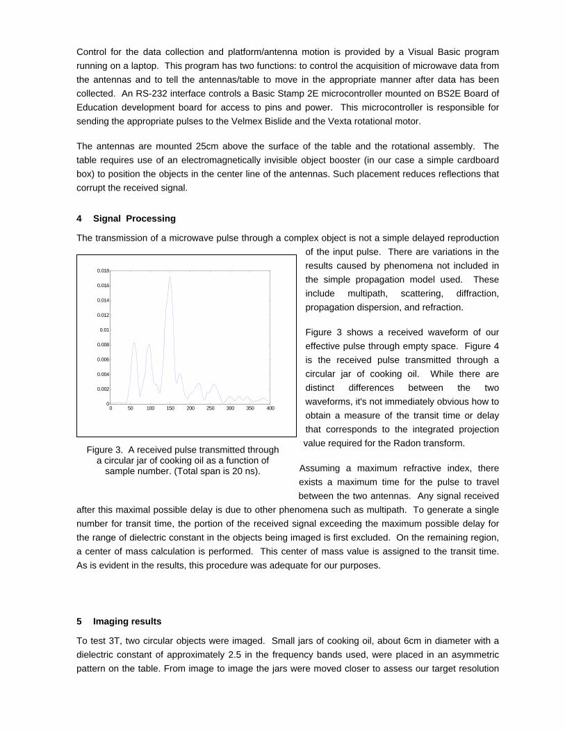
Figure 3. A received pulse transmitted through a circular jar of cooking oil as a function of

sample number. (Total span is 20 ns).

Control for the data collection and platform/antenna motion is provided by a Visual Basic program running on a laptop. This program has two functions: to control the acquisition of microwave data from the antennas and to tell the antennas/table to move in the appropriate manner after data has been collected. An RS-232 interface controls a Basic Stamp 2E microcontroller mounted on BS2E Board of Education development board for access to pins and power. This microcontroller is responsible for sending the appropriate pulses to the Velmex Bislide and the Vexta rotational motor.

The antennas are mounted 25cm above the surface of the table and the rotational assembly. The table requires use of an electromagnetically invisible object booster (in our case a simple cardboard box) to position the objects in the center line of the antennas. Such placement reduces reflections that corrupt the received signal.

4 Signal Processing

The transmission of a microwave pulse through a complex object is not a simple delayed reproduction of the input pulse. There are variations in the results caused by phenomena not included in the simple propagation model used. These include multipath, scattering, diffraction, propagation dispersion, and refraction.

Figure 3 shows a received waveform of our effective pulse through empty space. Figure 4 is the received pulse transmitted through a circular jar of cooking oil. While there are distinct differences between the two waveforms, it's not immediately obvious how to obtain a measure of the transit time or delay that corresponds to the integrated projection value required for the Radon transform.

Assuming a maximum refractive index, there exists a maximum time for the pulse to travel between the two antennas. Any signal received

after this maximal possible delay is due to other phenomena such as multipath. To generate a single number for transit time, the portion of the received signal exceeding the maximum possible delay for the range of dielectric constant in the objects being imaged is first excluded. On the remaining region, a center of mass calculation is performed. This center of mass value is assigned to the transit time. As is evident in the results, this procedure was adequate for our purposes.

5 Imaging results

To test 3T, two circular objects were imaged. Small jars of cooking oil, about 6cm in diameter with a dielectric constant of approximately 2.5 in the frequency bands used, were placed in an asymmetric pattern on the table. From image to image the jars were moved closer to assess our target resolution

limit. For a fixed object, the antennas linearly translate across the table in 500 increments. The object is rotated by the table and an additional 500 projections are taken. For the 180o range, 250 equally spaced angular increments are used. Therefore, 125,000 line projections are generated for each image.

In Figures 5 through 7, both the sinograms [Natterer] and reconstructed images are illustrated. The object’s actual position is indicated by the black outline. The vertical lines in the sinograms are discontinuities caused either by the table being accidentally bumped during the data collection process or other external interferences. In each case, the artifacts in the sinogram have not caused significant errors in the image reconstruction. Figure 8 shows the sinogram and image from a rectangular shaped piece of plastic.

These simple images are a first step in demonstrating the feasibility and utility of 3T. Our circular objects are well reconstructed at a resolution consistent with the microwave wavelengths being used and their placements in the image correspond very well to the actual positions of the jars of oil. The free space wavelength for the frequency range of the imaging energy ranged from 30 to 1.5 cm.

Figure 5. Sinogram (left) and reconstructed image (right) of two jars of oil, centers 15.24 cm apart.

0 50 100 150 200 250 300 350 4000

0.002

0.004

0.006

0.008

0.01

0.012

Figure 4. A received pulse transmitted through only air versus sample number. (Total span is 20 ns)

Figure 6. Sinogram (left) and reconstructed image (right) of two jars of oil, centers 10.16 cm apart.

Figure 7. Sinogram (left) and reconstructed image (right) of two jars of oil, centers 6.35 cm apart.

Figure 8. Sinogram (left) and reconstructed image (right) for a rectangular plastic block.

6 Conclusions and Comments

We have shown the feasibility of 3T via a fairly elementary measurement setup on simple targets. It is significant that the targets were imaged in air with no special considerations for signal corruption due to multipath and stray reflections. Objects more complex than simple dielectric cylinders will require more advanced signal processing to address errors introduced by these effects. A practical system will also require an array of antennas and much more rapid data acquisition.

References

Suetens, X. P., 2002, Fundamentals of Medical Imaging, Cambridge University Press. Prince, Y. J. L., Links, J., 2005, Medical Imaging Signals and Systems, Prentice Hall. Natterer, F., 2001, The Mathematics of Computerized Tomography, Cambridge University Press. Fear, E.C., Hagness, S.C., Meaney, P.M., Okonierski, M. and Stuchly, M.A., 2002 , “Enhancing Breast Tumor Detection with Near-Field Imaging,” IEEE Microwave Magazine, pp.48-56. Semenov S.Y., Bulyshev A.E., Abubakar A., Posukh V.G., Sizov, Y.E., Souvorov A.E., van den Berg P.M., Williams T.C., 2005, “Microwave-tomographic imaging of the high dielectric-contrast objects using different image-reconstruction approaches,” IEEE Transactions on Microwave Theory and Techniques, Volume 53, Issue 7, pp 2284 - 2294. Miyakawa M., Eiyama M., Ishii N, 2001,“An attempt of time domain microwave computed tomography for biomedical use” Engineering in Medicine and Biology Society, Proceedings of the 23rd Annual International Conference of the IEEE. Trumbo, M., 2006, A New Modality for Microwave Tomographic Imaging: Time Transit Tomography, M.S. Thesis, Baylor University. Ammon, C. J., and J. E. Vidale, 1993, Tomography without rays, Seismological Society of America Bulletin, 83, 509-528. Aldridge, D. F., and D. W., Oldenburg, D. W., 1993, Two-dimensional tomographic inversion with finite-difference traveltimes, Journal of Seismic Exploration, 2, 257-274. Berryman, J. G., 1989, Fermat's principle and nonlinear traveltime tomography, Physical Review Letters, 62, 2953-2956. Berryman, J. G., 1989, Weighted least-squares criteria for seismic traveltime tomography, IEEE Transactions on Geoscience and Remote Sensing, 27, 302-309. Bishop, T. N., Bube, K. P., Cutler, R. T., Langan, R. T., Love, P. L., Resnick, J. R., Shuey, R. T., Spindler, D. A., and Wyld, H. W., 1985, Tomographic determination of velocity and depth in laterally varying media, Geophysics, 50, 903-923. Bregman, N. D., Chapman, C. H., and Bailey, R. C., 1989, Travel time and amplitude analysis in seismic tomography, Journal of Geophysical Research, 94, 7577-7587. Delprat-Jannaud, F. and Lailly, P., 1992, Ill-posed and well-posed formulations of the reflection traveltime tomography problem, Journal of Geophysical Research, 97, 19827-19844. Eppstein, M. J. and Dougherty, D. E., 1998, Optimal 3-d traveltime tomography, Geophysics, 63, 1053-1061. Hole, J. A., 1992, Nonlinear high-resolution three-dimensional seismic travel time tomography, Journal of Geophysical Research, 97, 6553-6562.

Menke, W., 1984. Geophysical Data Analysis: Discrete Inverse Theory. Academic Press Michelena, R. J., and Harris, J. M., 1991, Tomographic traveltime inversion using natural pixels, Geophysics, 56, 635-644. Nemeth, T., Normark, E., and Qin, F., 1997, Dynamic smoothing in crosswell traveltime tomography, Geophysics, 62, 168-176. Nolet, G. (Ed.), 1987. Seismic Tomography with Applications in Global Seismology and Exploration Geophysics. Springer. Phillips, W. S., and Fehler, M. C., 1991, Traveltime tomography: A comparison of popular methods, Geophysics, 56, 1639-1649. Scales, J. A., Gersztenkorn, A., and Treitel, S., 1988, Fast lp solution of large, sparse, linear systems: Application to seismic travel time tomography Journal of Computational Physics, 75, 314-333. Schuster, G. T., Resolution limits for crosswell migration and traveltime tomography, Geophysical Journal International, 127, 427-440, 1996. Spakman, W., and Nolet, G., 1988, Imaging algorithms, accuracy and resolution in delay-time tomography, in Vlaar, N. J., G. Nolet, M. J. R. Wortel, et al. (eds.), Mathematical Geophysics, Hingham, MA: Reidel, 155-187. Vasco, D. W., Peterson, Jr., J. E., and Majer, E. L., 1996,Nonuniqueness in traveltime tomography: Ensemble inference and cluster analysis, Geophysics, 61, 1209-1227. Vasco, D. W., and Majer, E. L., 1993, Wavepath traveltime tomography, Geophysical Journal International, 115, 1055-1069. Washbourne, J. K., Rector, J. W., and Bube, K. P., 2002, Crosswell traveltime tomography in three dimensions, Geophysics, 67, 853-871. Zhang, J. and Toksoz, M. N., 1998, Nonlinear refraction traveltime tomography, Geophysics, 63, 1726-1737. Munk, W., Worcester, P., and Wunsch, C., 1995, Ocean Acoustic Tomography, Cambridge University Press, ISBN 0-521-47095-1. Shang, E. C., 1989, Ocean acoustic tomography based on adiabatic mode theory, The Journal of the Acoustical Society of America, Volume 85, Issue 4, pp. 1531-1537.