A New Look at Stratospheric Sudden Warmings. Part II

A New Look at Stratospheric Sudden Warmings. Part II: Evaluation of NumericalModel Simulations

ANDREW J. CHARLTON,*,@@ LORENZO M. POLVANI,� JUDITH PERLWITZ,# FABRIZIO SASSI,@ELISA MANZINI,& KIYOTAKA SHIBATA,** STEVEN PAWSON,�� J. ERIC NIELSEN,�� AND DAVID RIND##

*Department of Applied Physics and Applied Mathematics, Columbia University, New York, New York�Department of Applied Physics and Applied Mathematics, and Department of Earth and Environmental Sciences,

Columbia University, New York, New York#Cooperative Institute for Research in Environmental Sciences, Climate Diagnostics Center, University of Colorado, and Physical

Sciences Division, NOAA/Earth System Research Laboratory, Boulder, Colorado@National Center for Atmospheric Research, Boulder, Colorado&Istituto Nazionale di Geofisica e Vulcanologia, Bologna, Italy

**Meteorological Research Institute, Tsukuba, Ibaraki, Japan��Global Modeling and Assimilation Office, NASA GSFC, Greenbelt, Maryland

##NASA Goddard Institute for Space Studies, New York, New York

(Manuscript received 13 October 2005, in final form 28 March 2006)

ABSTRACT

The simulation of major midwinter stratospheric sudden warmings (SSWs) in six stratosphere-resolvinggeneral circulation models (GCMs) is examined. The GCMs are compared to a new climatology of SSWs,based on the dynamical characteristics of the events. First, the number, type, and temporal distribution ofSSW events are evaluated. Most of the models show a lower frequency of SSW events than the climatology,which has a mean frequency of 6.0 SSWs per decade. Statistical tests show that three of the six modelsproduce significantly fewer SSWs than the climatology, between 1.0 and 2.6 SSWs per decade. Second, fourprocess-based diagnostics are calculated for all of the SSW events in each model. It is found that SSWs inthe GCMs compare favorably with dynamical benchmarks for SSW established in the first part of the study.

These results indicate that GCMs are capable of quite accurately simulating the dynamics required toproduce SSWs, but with lower frequency than the climatology. Further dynamical diagnostics hint that, inat least one case, this is due to a lack of meridional heat flux in the lower stratosphere. Even though theSSWs simulated by most GCMs are dynamically realistic when compared to the NCEP–NCAR reanalysis,the reasons for the relative paucity of SSWs in GCMs remains an important and open question.

1. Introduction

In Part I of this study (Charlton and Polvani 2006,henceforth CP06), we constructed a new climatology ofmajor midwinter stratospheric sudden warmings(SSWs) and proposed benchmarks for their simulationin general circulation models (GCMs). In this study wewill analyze the simulation of SSWs by a series ofstratosphere-resolving GCMs. The GCMs will be

evaluated in two ways. First, the number, type, andclimatology of SSWs in the models will be compared tothe climatology established by CP06. Second, process-based benchmarks of SSWs, introduced by CP06, willbe used to assess the performance of each GCM.

Previous studies have examined the simulation ofSSWs by individual stratosphere-resolving GCMs (e.g.,Butchart et al. 2000; Manzini and Bengtsson 1996;Erlebach et al. 1995), but as far as we are aware therehas been no comprehensive intercomparison of the per-formance of a series of GCMs in this respect. Most ofthe recent intercomparisons of stratosphere-resolvingGCMs (e.g., Austin et al. 2003; Shine et al. 2003) havetouched only briefly on the simulation of SSWs.

The occurrence of SSWs is crucial to the chemistry ofozone, since the low temperatures that occur in undis-turbed winters are an important prerequisite for deni-

@@ Current affiliation: Department of Meteorology, Universityof Reading, Reading, United Kingdom.

Corresponding author address: Andrew J. Charlton, Depart-ment of Meteorology, University of Reading, Reading, Berkshire,RG6 6BB, United Kingdom.E-mail: [email protected]

470 J O U R N A L O F C L I M A T E VOLUME 20

© 2007 American Meteorological Society

JCLI3994

trification and subsequent catalytic ozone loss, if thevortex remains intact into the spring. The importanceof warmings was recognized early in the GCM RealityIntercomparison Project for SPARC (GRIPS) modelevaluation (Pawson et al. 2000), but the restrictedlength of model simulations available until quite re-cently has precluded detailed examination of the fre-quency of occurrence of simulated SSWs. With longerruns of coupled Chemistry–Climate Models (CCMs)now possible, the CCM Validation (CCMVal) project(Eyring et al. 2005) will examine SSWs in more detail.This study, along with CP06, should complement andinform CCMVal, both by assessing the performance ofsome GCMs and by suggesting process-based dynami-cal benchmarks to test other GCMs.

Part of the interest in validating stratosphere-resolving GCMs is also due to the potential interactionsbetween greenhouse gas–induced climate changes,stratospheric ozone depletion, and dynamical couplingbetween the stratosphere and troposphere (Hartmannet al. 2000). There is little consensus about futurechanges to variability of the Arctic stratospheric polarvortex (Rind et al. 1998; Schnadt and Dameris 2003).We surmise that a necessary though not sufficient con-dition for the suitability of GCMs to accurately simu-late future stratospheric variability is that they producea credible simulation of the current SSW climatology.Other factors, such as the simulation of future tropo-spheric variability, should also be considered when de-termining the suitability of a GCM for this task.

The paper is structured as follows. The GCMs to beanalyzed and the methods used are described in section2. In section 3 we compare the stratospheric climatol-ogy of the GCMs. In section 4 we examine the number,type, and climatology of SSWs. In section 5 we compareprocess-based benchmarks of SSWs between theGCMs. In section 6 we provide further discussion andcomparison of the stratospheric dynamics of eachGCM. In section 7 we present conclusions.

2. Methodology and GCM runs

This section briefly describes the methodology usedto identify and classify SSWs and gives brief details ofthe GCMs used in the study. Neither discussion is in-tended to be exhaustive and readers should consult rel-evant references for further details.

The methodology for identifying and classifyingSSWs is described in full by CP06. We confine our studyto SSWs that occur during the extended winter season,November to March. First, SSWs are defined to occurwhen the zonal mean zonal wind at 10 hPa and 60°Nbecomes easterly, in line with the WMO definition. Anadditional criterion, that the zonal mean zonal winds

return to westerlies for 10 or more consecutive daysfollowing the SSW, is used to remove events that arefinal warmings. Second, the algorithm classifies SSWsinto vortex splits (in which the stratospheric polar vor-tex breaks into two comparably sized pieces) and vor-tex displacements (in which the vortex remains largelyintact). The algorithm uses absolute vorticity to identifythe vortex edge and then compares the size andstrength of cyclonically rotating vortices in the flow todetermine if events are vortex splits or vortex displace-ments.

In CP06, data from both the National Centers forEnvironmental Prediction–National Center for Atmo-spheric Research (NCEP–NCAR) reanalysis (Kistler etal. 2001), and its Climate Data Assimilation System(CDAS) extension, and the 40-yr European Centre forMedium-Range Weather Forecasts (ECMWF) Re-Analysis (ERA-40) dataset (Kallberg et al. 2004) wereused to establish a climatology of SSWs events betweenthe winter seasons of 1957/58 and 2001/02. The resultsfrom the two reanalysis datasets were found to be verysimilar, as should be expected given their largely com-mon source of observations. Therefore in the presentstudy we use only the NCEP–NCAR data to evaluatethe GCMs. This also makes the construction of many ofthe statistical tests much simpler.

The CP06 algorithm was used to test the simulationof SSWs in a series of GCM simulations. We studyGCMs that are explicitly designed to resolve the strato-sphere, which we call stratosphere resolving. We definestratosphere-resolving GCMs as those with a model topclose to or above the stratopause (approximately 50 kmor 0.8 hPa) and with a meaningful number of modellevels (10 or more) in the stratosphere. One major con-straint in choosing and obtaining GCM integrations inorder to examine the intra-annual variability of SSWs isthat daily or finer time resolution of diagnostic fields isrequired. We found that the archiving of daily output isby no means a standard practice among the modelingcenters and groups that run stratosphere-resolvingGCMs.

The GCMs used in this study are summarized inTable 1, and the forcings used in each model are shownin Table 2. In the following subsections we briefly dis-cuss each GCM. We have attempted to restrict our at-tention in this study to GCM runs that are forced by seasurface temperatures (SSTs) from the same time periodas the NCEP–NCAR reanalysis. It was not possible toobtain runs with observed SSTs for the MeteorologicalResearch Institute/Japan Meteorological Agency 1998Model (MRIJMA; run with climatological SSTs), andthis may be a potential source of bias.

We have also attempted to examine the longest avail-

1 FEBRUARY 2007 C H A R L T O N E T A L . 471

able runs of each GCM, to try to avoid spurious dis-agreement between the GCMs and reanalysis resultingfrom potential decadal variability of SSWs (Butchart etal. 2000). Except for the Middle Atmosphere ECHAMModel (MAECHAM; which is run for 29 full winterseasons), all of the GCM runs used here are over com-parable or longer time periods than the reanalysis data,typically 50 yr.

a. NASA Goddard Space Flight Center,finite-volume GCM (FVGCM)

The National Aeronautics and Space Administration(NASA) Goddard Earth Observing System (GEOS-4)GCM is a middle-atmosphere GCM based on the finite-volume dynamical core of Lin (2004), with gravity wavedrag, cloud, and cumulus parameterizations originallybased on those in the Community Atmosphere Modelversion 3 (CAM3). The model has 55 levels in the ver-tical and the model top is at 0.01 hPa (approximately 80km); the average vertical spacing of levels in the strato-sphere is 1.2 km. The model has a flexible horizontalresolution and is run in this case at 2° � 2.5°. The modelis forced with observed SSTs and sea ice between 1949and 1997 using the Rayner et al. (2003) dataset. Themodel runs are described in more detail in Stolarski etal. (2005).

b. NASA Goddard Institute for Space Studies,Global Climate/Middle Atmosphere Model, newversion (GISSL53)

The new NASA Goddard Institute for Space Studies,Global Climate/Middle Atmosphere Model 3 is an up-

date from the previous version of the Global Climate–Middle Atmosphere Model (GCMAM; Rind et al.2002). The update includes new boundary layer andturbulent schemes, convective and cloud cover param-eterizations, and atmospheric radiation code. Thebroad nature of the changes to these schemes is sharedwith the new GISS model-E (Schmidt et al. 2006). Thegravity wave drag in this model utilizes the formula-tions discussed in Rind et al. (1999, 1988) except thatmuch smaller values are used. A major difference withthe other models is that the nonorographic gravity wavedrag components are a function of resolved processes inthe troposphere. The model has four different verticaland horizontal resolutions; the version used here is 4° �5°, with 53 layers in the vertical and model top at 0.002hPa (approximately 85 km). The vertical spacing is 500m in the middle to upper troposphere, 0.5 to 1 km in thelower stratosphere, and 2 to 2.5 km in the upper strato-sphere. The model is forced with observed SSTs andsea ice between 1951 and 1997 using the Rayner et al.(2003) dataset. A more complete description of all theversions of the model is given in Rind et al. (2006,manuscript submitted to J. Geophys. Res.).

c. NASA Goddard Institute for Space Studies,Global Climate/Middle Atmosphere Model,legacy version (GISSL23)

The NASA GISS Global Climate/Middle Atmo-sphere Model is a middle-atmosphere GCM based onthe climate model of Hansen et al. (1983) and themiddle-atmosphere version outlined by Rind et al.

TABLE 2. Forcings used in each GCM run.

GCM Sea ice extentCO2

conc./ppmv O3 climatologySolar forcingTOA/W m�2

FVGCM Obs 1949–97 (Rayner et al. 2003) Fixed 355 Monthly variance (Langematz 2000) Fixed 1367GISSL53 Climate 1975–84 (Rayner et al. 2003) Fixed 311 Monthly and yearly variance; multiple

sources (see text)Fixed 1365.5

GISSL23 Climate 1975–84 (Rayner et al. 2003) Fixed 311 Monthly variance (London et al. 1976) Fixed 1367.6WACCM Obs 1951–2000 (NCEP–NCAR, Reynolds) Fixed 355 Monthly variance (Liang et al. 1997) Fixed 1367MAECHAM Obs 1970–98 (Rayner et al. 2003) Fixed 348 Monthly variance (Fortuin and Kelder 1998) Fixed 1365MRIJMA Climate 1978–98 (Rayner et al. 2003) Fixed 348 Monthly variance (Liang et al. 1997)

(�0.4 hPa) CIRA (�0.4 hPa)Fixed 1365

TABLE 1. GCM experiments used in the study.

GCMRun

length/winters SST forcingHorizontalresolution

Verticallevels Model top Reference

FVGCM 49 Obs 1949–97 2° � 2.5° 55 0.01 hPa Stolarski et al. (2005)GISSL53 47 Obs 1951–97 4° � 5° 53 0.002 hPa Rind et al. (2002)GISSL23 46 Obs 1951–96 8° � l0° 23 0.002 hPa Shindell et al. (1998)WACCM 50 Obs 1951–2000 T63 66 150 km Sassi et al. (2004)MAECHAM 29 Obs 1970–98 T42 39 0.01 hPa Manzini et al. (2006)MRIJMA 60 Climate 60 years T42 45 0.01 hPa Shibata et al. (1999)


(1988). The model has 23 levels in the vertical and themodel top is at 0.002 hPa (approximately 85 km). Thevertical spacing of levels is 0.2 km near the surface, 3.8km in the upper troposphere, and 5 to 5.8 km in thestratosphere. The model has a horizontal resolution of8° � 10°. The model is forced with observed SSTs andsea ice between 1951 and 1997 using the Rayner et al.(2003) dataset. GISSL23 has a much coarser horizontaland vertical resolution than most of the other models inthe study. We include it because it has been used in anumber of high-profile studies that examined the re-sponse of the stratosphere to changing greenhouse gasconcentrations and the impact of these changes on thetropospheric flow (e.g., Shindell et al. 1999). Note thatthis version of the model differs from that used in Rindet al. (1988) and subsequent publications in that it hasgreatly reduced orographic drag (Shindell et al. 1998).

d. NCAR Whole Atmosphere Community ClimateModel (WACCM)

The NCAR Whole Atmosphere Community ClimateModel version 1b is an extended version of the NCARCommunity Climate Model version 3 (CCM3; Kiehl etal. 1998). The model has 66 levels in the vertical and themodel top is at 150 km (approximately 0.000002 hPa).The average vertical spacing of levels in the strato-sphere is 1.5 km. The model has a spectral formulation,with resolution of T63 (approximately 1.875° � 1.875°).The model is forced with observed SSTs from 1950 to2000 using the NCEP Reynolds observed dataset(http://podaac.jpl.nasa.gov/reynolds). The model runsare described in more detail in Sassi et al. (2004).

e. Max Planck Institute for Meteorology(MPI)/Middle Atmosphere ECHAM Model(MAECHAM)

The MPI MAECHAM model is an extended versionof the MPI ECHAM5 model (Roeckner et al. 2003).The model has 39 levels in the vertical and the modeltop is at 0.01 hPa (approximately 80 km). The verticalspacing of levels in the stratosphere varies from 1.5 to 3km. The model has a spectral formulation, with resolu-tion of T42 (approximately 2.8° � 2.8°). The model isforced with observed SST and sea ice forcings, from theAtmospheric Model Intercomparison Project II (AMIPII; Gates et al. 1999). The model is described in moredetail by Manzini et al. (2006).

f. The Meteorological Research Institute/JapaneseMeteorological Agency 1998 Model (MRIJMA)

The MRIJMA 1998 Model is a hybrid version of theMeteorological Research Institute model (Chiba et al.

1996) and the operational global model (GSM9603) ofthe Japan Meteorological Agency (JMA 1997). Themodel has 45 levels in the vertical and the model top isat 0.01 hPa (approximately 80 km). The average verti-cal spacing of levels in the stratosphere is 2 km. Themodel has a spectral formulation, with resolution ofT42 (approximately 2.8° � 2.8°). The model is forcedwith climatological SSTs and run for 60 yr. The modelsetup is described in more detail in Shibata et al. (1999).The climatological SSTs are 21-yr averages between1978 and 1998, based on the Hadley Centre SST dataset(HadSST).

3. Climatology of GCMs

In this section, the stratospheric climatology of theGCMs is briefly examined. An indication of thestrength and size of the stratospheric polar vortex ineach GCM can be gained by examining the strato-spheric climatology, with the caveat that it is often dif-ficult to separate the time and zonal mean state of thestratosphere and its time-varying component. We re-strict our analysis to the zonal mean zonal wind at 10hPa and the meridional heat flux at 100 hPa both forsake of brevity and because of the limited amount ofdata available to us.

a. Zonal mean zonal wind at 10 hPa

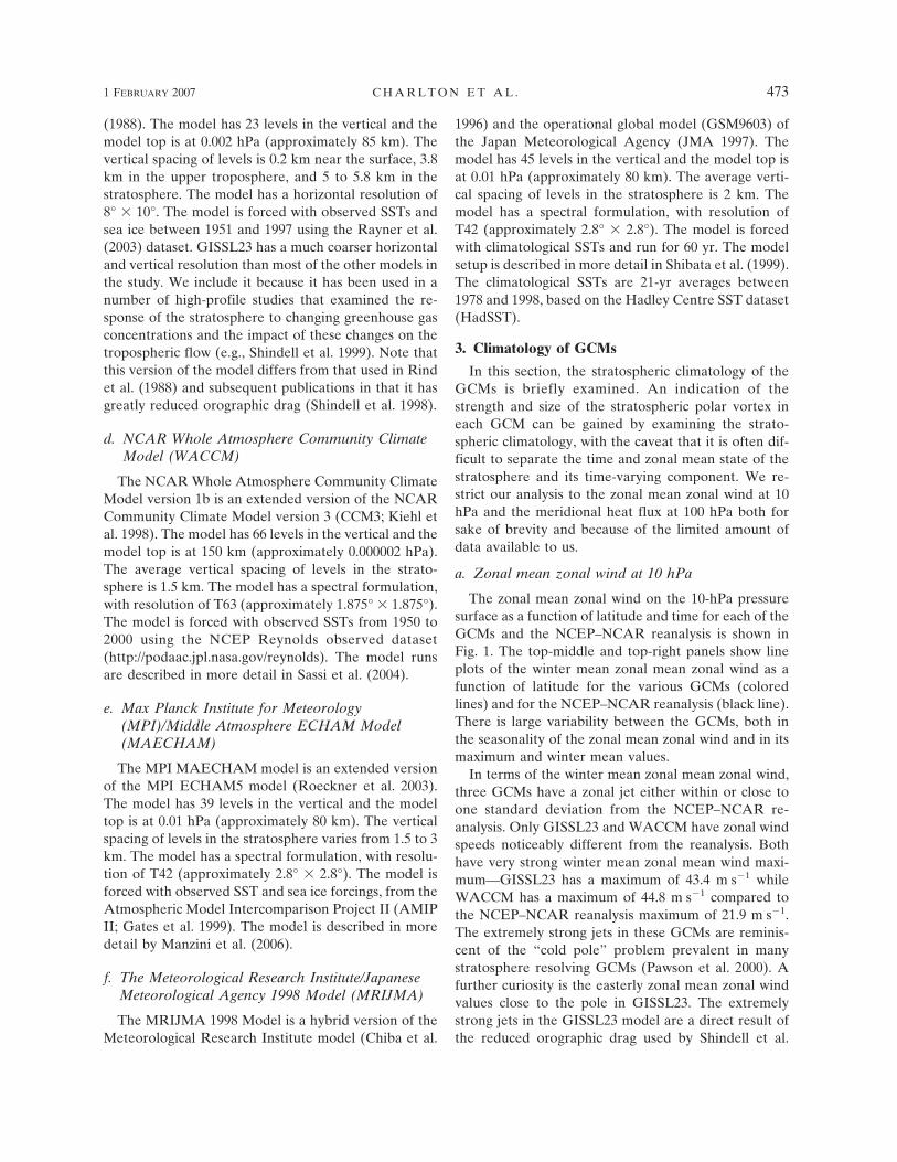
The zonal mean zonal wind on the 10-hPa pressuresurface as a function of latitude and time for each of theGCMs and the NCEP–NCAR reanalysis is shown inFig. 1. The top-middle and top-right panels show lineplots of the winter mean zonal mean zonal wind as afunction of latitude for the various GCMs (coloredlines) and for the NCEP–NCAR reanalysis (black line).There is large variability between the GCMs, both inthe seasonality of the zonal mean zonal wind and in itsmaximum and winter mean values.

In terms of the winter mean zonal mean zonal wind,three GCMs have a zonal jet either within or close toone standard deviation from the NCEP–NCAR re-analysis. Only GISSL23 and WACCM have zonal windspeeds noticeably different from the reanalysis. Bothhave very strong winter mean zonal mean wind maxi-mum—GISSL23 has a maximum of 43.4 m s�1 whileWACCM has a maximum of 44.8 m s�1 compared tothe NCEP–NCAR reanalysis maximum of 21.9 m s�1.The extremely strong jets in these GCMs are reminis-cent of the “cold pole” problem prevalent in manystratosphere resolving GCMs (Pawson et al. 2000). Afurther curiosity is the easterly zonal mean zonal windvalues close to the pole in GISSL23. The extremelystrong jets in the GISSL23 model are a direct result ofthe reduced orographic drag used by Shindell et al.


(1998) and are not a characteristic of the model as nor-mally used (e.g., Rind et al. 1988, their Figs. 2 and 3).Only GISSL53 has a weaker winter mean zonal meanwind maximum (17.6 m s�1) than the reanalysis.

The seasonal cycle [Fig. 1 and further analysis (notshown)] varies markedly between the different GCMs.The reanalysis shows peak zonal mean zonal winds inthe extratropics between days 50 and 80 of the winterseason (late December to early February). Three of the

models (FVGCM, WACCM, and MRIJMA) simulatethis seasonality correctly, although the absolute valuesof the zonal mean zonal wind in WACCM are on av-erage 15 m s�1 larger than the NCEP–NCAR reanaly-sis. GISSL53 has a seasonality shifted toward early win-ter, with peak zonal mean zonal winds between days 10and 30 (November). MAECHAM has a seasonalityshifted toward late winter, with peak zonal mean zonalwinds between days 80 and 110 (late January to Feb-

FIG. 1. Zonal mean zonal wind climatology at 10 hPa for GCMs that resolve the stratosphere in this study. (top left) Climatology fromNCEP–NCAR reanalysis for the years 1958–2002. Contour interval is 5 m s�1. (top middle), (top right) Line plots show winter meanfor each GCM: NCEP–NCAR climatology in thick black line, FVGCM in red line, GISSL53 in green line, GISSL23 in blue line,WACCM in magenta line, MAECHAM in the cyan line, and MRIJMA in yellow line. Gray shading shows �one interannual standarddeviation from the mean.


Fig 1 live 4/C

ruary). GISSL23 has a much broader zonal mean zonalwind peak than the reanalysis or the other models, withlarge relative zonal wind speeds throughout February.Most of the models simulate the climatology of Marchand April well, although GISSL53 has absolute valuesof zonal mean wind speed at 60°N and 10 hPa slightlysmaller than the reanalysis in early March. It is alsonoticeable that in both GISS23 and WACCM the finalwarming is much later than in other GCMs or theNCEP–NCAR reanalysis. Also note that none of themodels produces a recognizable quasi-biennial oscilla-tion (QBO).

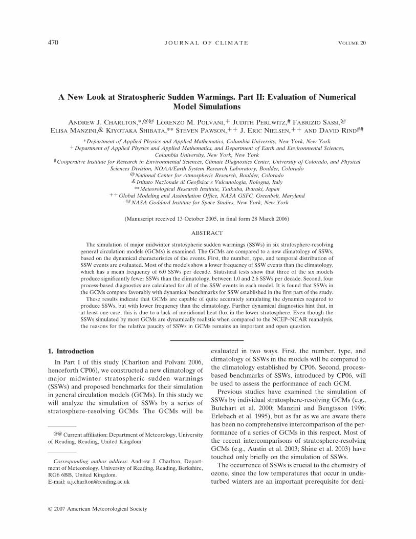
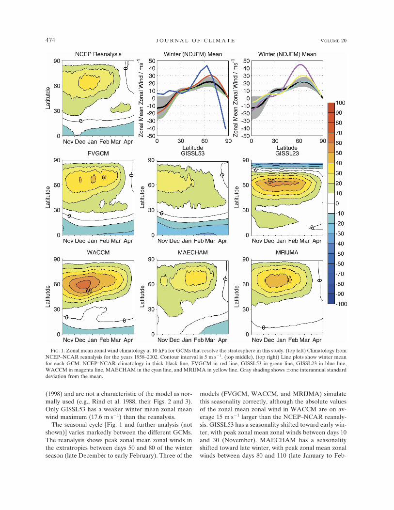
b. Meridional heat flux at 100 hPa

Throughout the rest of this study, the meridionalheat flux (��T�) will be used as a proxy for the verticalcomponent of the Eliassen–Palm flux, following Pol-vani and Waugh (2004). We use the meridional heatflux, rather than the full Eliassen–Palm flux (Andrewset al. 1985), as we were only able to obtain limitedamounts of data on daily time scales. In particular, onlyinformation on 100- and 10-hPa pressure surfaces wasobtained, making it impossible to calculate verticalderivatives, which are required to calculate the fullEliassen–Palm flux.

The meridional heat flux climatology (Fig. 2) at 100hPa is noisy, even in the NCEP–NCAR reanalysis plot,highlighting its large interannual variability. TheNCEP–NCAR meridional heat flux has a very broadseasonality, with large values occurring between mid-November and early March. Peak values of heat fluxare centered at 60°N throughout winter. The meridi-onal heat flux at 100 hPa is well simulated by most ofthe GCMs. Apart from GISSL23, the seasonality is wellsimulated. WACCM and MRIJMA have a heat fluxclimatology peaked too strongly in midwinter withlarge values in December and January, but their win-tertime means are very close to the NCEP–NCAR cli-matology.

Only the two GISS GCMs show major differenceswith the NCEP–NCAR climatology. GISSL53 has avery broad band of positive heat flux and a peak lo-cated approximately 10 degrees of latitude south of thepeak in the NCEP–NCAR reanalysis. GISSL23 hasvery weak heat flux throughout the year, and a winter-time mean peak heat flux less than 50% that of theNCEP–NCAR reanalysis. Part of this discrepancy maybe due to the relatively coarser horizontal resolution inthe GISS models.

4. Stratospheric warmings in the GCMs

In this section GCMs are evaluated by comparing thestatistics of SSWs with the statistics obtained from the

NCEP–NCAR reanalysis, which can be found in Table2 of CP06.

a. Frequency of major midwinter warmings

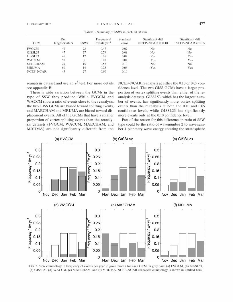
The number of SSWs in the GCM simulations isshown in Table 3. We compare the mean frequency ofSSWs per winter to take into account the differentlength of each GCM run and the reanalysis dataset.Column 2 shows the length of the model run, column 3shows the number of SSWs recorded, and column 4shows the expected frequency of SSWs per winter. Thestandard error of the frequency estimate is shown incolumn 5. A t test is used to determine which modelshave a significantly different frequency of SSWs com-pared to the NCEP–NCAR reanalysis dataset. Formore details of the statistical procedure see appendixA. Columns 5 and 6 show if the frequency of SSWs ineach model is significantly different from the frequencyof SSWs in the NCEP–NCAR reanalysis at significancelevels of 0.10 and 0.05.

Most of the GCMs in the present study have a lowerfrequency of SSWs than the reanalysis datasets. Of thesix GCM simulations, only one, GISSL53, has a higherfrequency of SSWs than the reanalysis datasets. Threeof the five GCMs that underestimate the frequencyof SSWs are significantly deficient at both the 0.10and 0.05 confidence levels (GISSL23, WACCM, andMRIJMA). In broad terms, models with a stronger po-lar vortex than the reanalysis (see Fig. 1) have a lack ofSSWs (GISSL23 and WACCM) and those with aweaker polar vortex than the reanalysis have an excessof SSWs (GISSL53, although not significantly so). Theexception to this is MRIJMA, but the lack of SSWshere may be related to the climatological SST forcing.

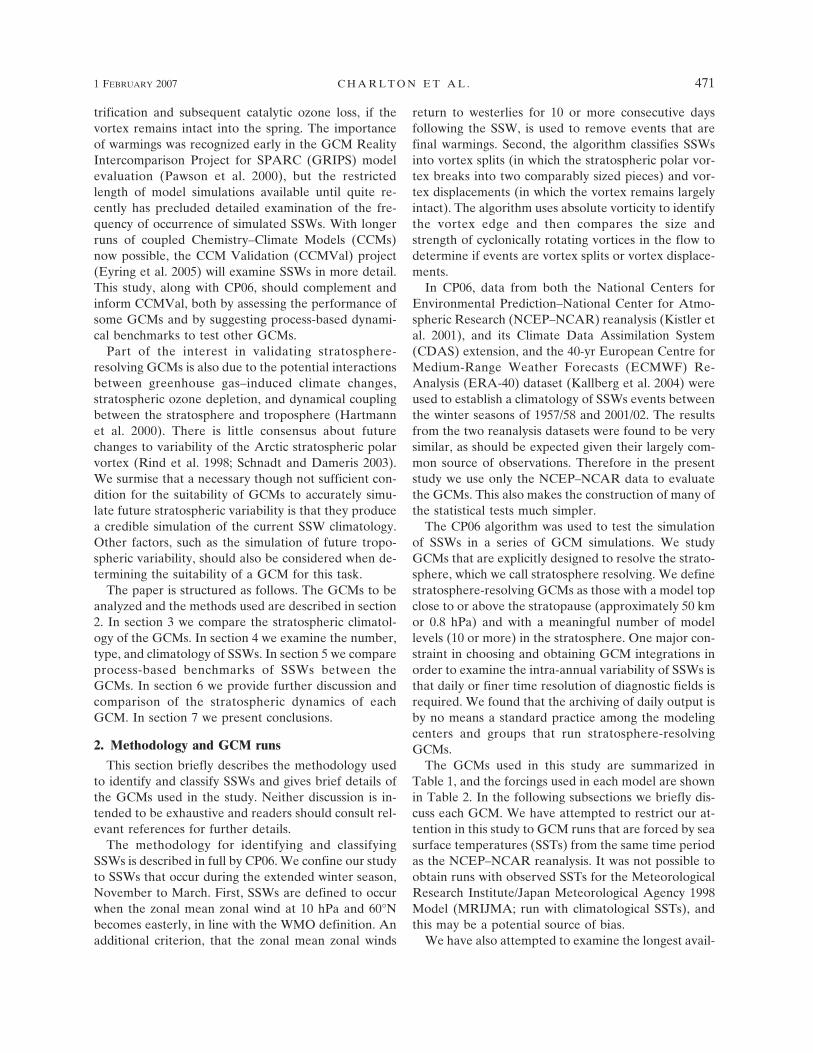
b. Climatology of warmings

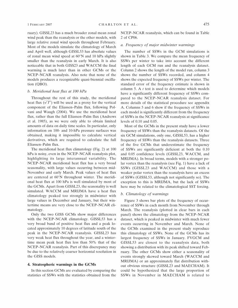
Figure 3 shows bar plots of the frequency of occur-rence of SSWs in each month from November throughMarch. The reanalysis (plotted in clear bars in eachpanel) shows the climatology from the NCEP–NCARdataset, which is peaked in midwinter with much fewerevents occurring in November and March. None ofthe GCMs examined in the present study reproducethis climatology of SSWs. None of the GCMs has itslargest frequency of SSWs in January. FVGCM andGISSL53 are closest to the reanalysis data, bothshowing a distribution with its peak shifted toward Feb-ruary. The other GCMs show either a seasonality ofevents strongly skewed toward March (WACCM andMRIJMA) or an approximately flat distribution with-out obvious structure (GISSL23 and MAECHAM). Itcould be hypothesized that the large proportion ofSSWs in November in MAECHAM is related to


MAECHAM’s relatively weak zonal mean zonal windsduring November (Fig. 1). Weak, climatological zonalmean zonal winds during February might also explainthe large number of SSWs in GISSL53 during Febru-ary. Two of the models with a lack of SSWs and arelatively strong zonal mean zonal wind jet at 10 hPaalso have SSWs mostly toward the end of winter(WACCM and GISSL23).

c. Type of warmings

The type of SSWs in the GCM runs is shown in Table4. In comparing the type of SSWs between the datasets

we disregard the number of events and focus on theratio between the number of vortex splits and vortexdisplacements. Column 2 shows the number of SSWs ineach model, column 3 shows the number of vortex dis-placements, and column 4 shows the vortex splits. Col-umn 5 shows the ratio between the number of vortexdisplacements and vortex splits. Columns 6 and 7 showif the distribution of vortex displacements and splits ineach model is significantly different from the distribu-tion in the NCEP–NCAR reanalysis. To statisticallycompare the type of events in each GCM, we constructbivariate tables of each GCM and the NCEP–NCAR

FIG. 2. Same as in Fig. 1, but for meridional heat flux climatology at 100 hPa. Contour interval is 5 K m s�1.


Fig 2 live 4/C

reanalysis dataset and use an 2 test. For more detailssee appendix B.

There is wide variation between the GCMs in thetype of SSW they produce. While FVGCM andWACCM show a ratio of events close to the reanalysis,the two GISS GCMs are biased toward splitting events,and MAECHAM and MRIJMA are biased toward dis-placement events. All of the GCMs that have a smallerproportion of vortex splitting events than the reanaly-sis datasets (FVGCM, WACCM, MAECHAM, andMRIJMA) are not significantly different from the

NCEP–NCAR reanalysis at either the 0.10 or 0.05 con-fidence level. The two GISS GCMs have a larger pro-portion of vortex splitting events than either of the re-analysis datasets. GISSL53, which has the largest num-ber of events, has significantly more vortex splittingevents than the reanalysis at both the 0.10 and 0.05confidence levels, while GISSL23 has significantlymore events only at the 0.10 confidence level.

Part of the reason for this difference in ratio of SSWtype could be the ratio of wavenumber 2 to wavenum-ber 1 planetary wave energy entering the stratosphere

FIG. 3. SSW climatology in frequency of events per year in given month for each GCM, in gray bars: (a) FVGCM, (b) GISSL53,(c) GISSL23, (d) WACCM, (e) MAECHAM, and (f) MRIJMA. NCEP–NCAR reanalysis climatology is shown in unfilled bars.

TABLE 3. Summary of SSWs in each GCM run.

GCMRun

length/winters SSWsFrequency/events yr�1

Standarderror

Significant diffNCEP–NCAR at 0.10


FVGCM 49 23 0.47 0.09 No NoGISSL53 47 37 0.79 0.08 No NoGISSL23 46 12 0.26 0.07 Yes YesWACCM 50 5 0.10 0.04 Yes YesMAECHAM 29 15 0.52 0.10 No NoMRIJMA 60 14 0.23 0.06 Yes YesNCEP–NCAR 45 27 0.60 0.10


in each GCM. Column 8 in Table 4 shows the climato-logical ratio of area-weighted, winter-mean meridionalheat flux between 45° and 75°N at 100 hPa due towavenumber 2 and due to wavenumber 1 in each ofthe GCMs and the NCEP–NCAR reanalysis dataset.MRIJMA, which has a large bias toward vortex dis-placement events, also has a large bias toward wave-number 1 heat flux compared to the reanalysis, whileGISSL23, which has a large bias toward vortex splittingevents also has a large bias toward wavenumber 2 heatflux compared to the reanalysis. However, for the otherGCMs this pattern does not hold and the reasons forthe SSW-type biases in the GCMs seem more compli-cated than the initial hypothesis expressed here.

5. Process-based performance of GCMs

In this section the dynamical benchmarks for SSWsestablished in CP06 are calculated for the SSWs foundin each of the GCM runs in the present study. In allfigures in this section, the distribution of benchmarks isshown with a box plot. The box of each plot shows theinterquartile range. The central line of the box showsthe median. The whiskers of the box show the minimumand maximum points in the distribution that are notoutliers. Outliers are marked with an “x” and are de-fined as any points that are greater than 3/2 times theinterquartile range from the ends of the box. The meanvalue of the diagnostic is shown by a cross. If the meanof the diagnostic in the GCM is significantly different at95% confidence from the mean of the diagnostic in thereanalysis dataset, the mean is plotted with a filledcircle. The mean of the diagnostic in each GCM and thereanalysis is compared with a standard two-sample ttest with unequal variances [see appendix A, Eqs.(A3)–(A4)].

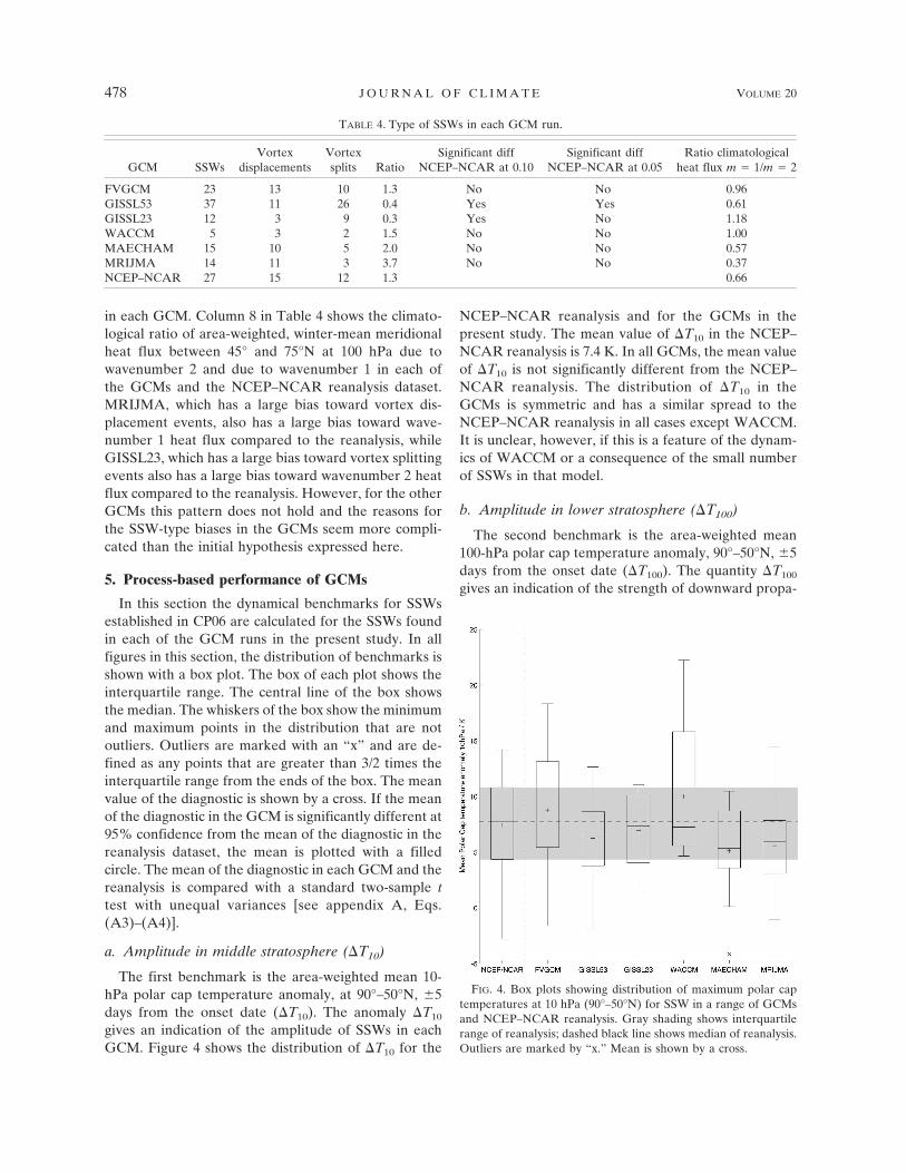
a. Amplitude in middle stratosphere (T10)

The first benchmark is the area-weighted mean 10-hPa polar cap temperature anomaly, at 90°–50°N, �5days from the onset date (T10). The anomaly T10

gives an indication of the amplitude of SSWs in eachGCM. Figure 4 shows the distribution of T10 for the

NCEP–NCAR reanalysis and for the GCMs in thepresent study. The mean value of T10 in the NCEP–NCAR reanalysis is 7.4 K. In all GCMs, the mean valueof T10 is not significantly different from the NCEP–NCAR reanalysis. The distribution of T10 in theGCMs is symmetric and has a similar spread to theNCEP–NCAR reanalysis in all cases except WACCM.It is unclear, however, if this is a feature of the dynam-ics of WACCM or a consequence of the small numberof SSWs in that model.

b. Amplitude in lower stratosphere (T100)

The second benchmark is the area-weighted mean100-hPa polar cap temperature anomaly, 90°–50°N, �5days from the onset date (T100). The quantity T100

gives an indication of the strength of downward propa-

FIG. 4. Box plots showing distribution of maximum polar captemperatures at 10 hPa (90°–50°N) for SSW in a range of GCMsand NCEP–NCAR reanalysis. Gray shading shows interquartilerange of reanalysis; dashed black line shows median of reanalysis.Outliers are marked by “x.” Mean is shown by a cross.

TABLE 4. Type of SSWs in each GCM run.

GCM SSWsVortex

displacementsVortexsplits Ratio



Ratio climatologicalheat flux m � 1/m � 2

FVGCM 23 13 10 1.3 No No 0.96GISSL53 37 11 26 0.4 Yes Yes 0.61GISSL23 12 3 9 0.3 Yes No 1.18WACCM 5 3 2 1.5 No No 1.00MAECHAM 15 10 5 2.0 No No 0.57MRIJMA 14 11 3 3.7 No No 0.37NCEP–NCAR 27 15 12 1.3 0.66


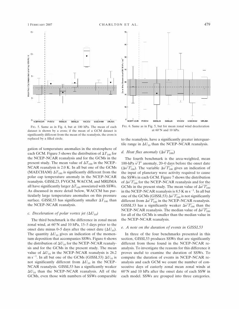
gation of temperature anomalies in the stratosphere ofeach GCM. Figure 5 shows the distribution of T100 forthe NCEP–NCAR reanalysis and for the GCMs in thepresent study. The mean value of T100 in the NCEP–NCAR reanalysis is 2.0 K. In all but one of the GCMs(MAECHAM) T100 is significantly different from thepolar cap temperature anomaly in the NCEP–NCARreanalysis. GISSL23, FVGCM, WACCM, and MRIJMAall have significantly larger T100 associated with SSWs.As discussed in more detail below, WACCM has par-ticularly large temperature anomalies on this pressuresurface. GISSL53 has significantly smaller T100 thanthe NCEP–NCAR reanalysis.

c. Deceleration of polar vortex jet (U10)

The third benchmark is the difference in zonal meanzonal wind, at 60°N and 10 hPa, 15–5 days prior to theonset date minus 0–5 days after the onset date (U10).The quantity U10 gives an indication of the momen-tum deposition that accompanies SSWs. Figure 6 showsthe distribution of U10 for the NCEP–NCAR reanaly-sis and for the GCMs in the present study. The meanvalue of U10 in the NCEP–NCAR reanalysis is 26.2m s�1. In all but one of the GCMs (GISSL53) U10 isnot significantly different from U10 in the NCEP–NCAR reanalysis. GISSL53 has a significantly weakerU10 than the NCEP–NCAR reanalysis. All of theGCMs, even those with numbers of SSWs comparable

to the reanalysis, have a significantly greater interquar-tile range in U10 than the NCEP–NCAR reanalysis.

d. Heat flux anomaly (��T�100)

The fourth benchmark is the area-weighted, mean100-hPa ��T� anomaly, 20–0 days before the onset date(��T�100). The variable ��T�100 gives an indication ofthe input of planetary wave activity required to causethe SSWs in each GCM. Figure 7 shows the distributionof ��T�100 for the NCEP–NCAR reanalysis and for theGCMs in the present study. The mean value of ��T�100

in the NCEP–NCAR reanalysis is 8.5 K m s�1. In all butone of the GCMs (GISSL53) ��T�100 is not significantlydifferent from ��T�100 in the NCEP–NCAR reanalysis.GISSL53 has a significantly weaker ��T�100 than theNCEP–NCAR reanalysis. The median value of ��T�100

for all of the GCMs is smaller than the median value inthe NCEP–NCAR reanalysis.

e. A note on the duration of events in GISSL53

In three of the four benchmarks presented in thissection, GISSL53 produces SSWs that are significantlydifferent from those found in the NCEP–NCAR re-analysis. To investigate the reasons for this difference itproves useful to examine the duration of SSWs. Tocompute the duration of events in NCEP–NCAR re-analysis and each GCM we count the number of con-secutive days of easterly zonal mean zonal winds at60°N and 10 hPa after the onset date of each SSW ineach model. SSWs are grouped into three categories.

FIG. 5. Same as in Fig. 4, but at 100 hPa. The mean of eachdataset is shown by a cross; if the mean of a GCM dataset issignificantly different from the mean of the reanalysis, the cross isreplaced by a filled circle.

FIG. 6. Same as in Fig. 5, but for mean zonal wind decelerationat 60°N and 10 hPa.


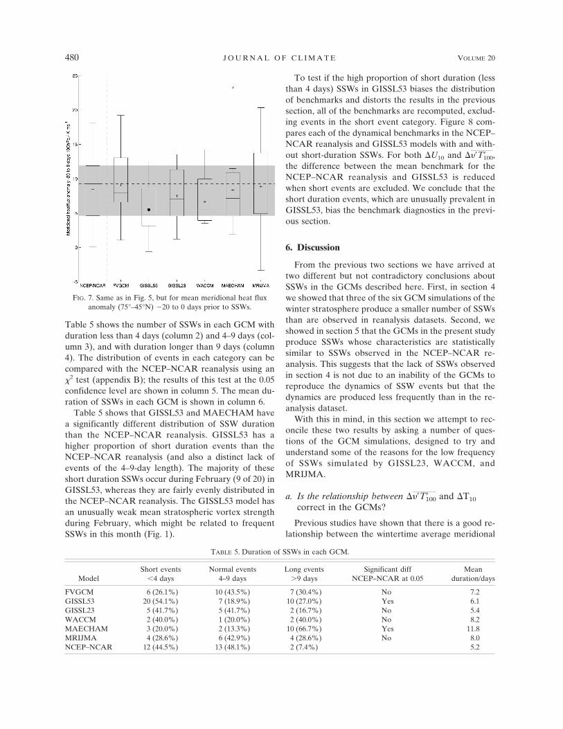
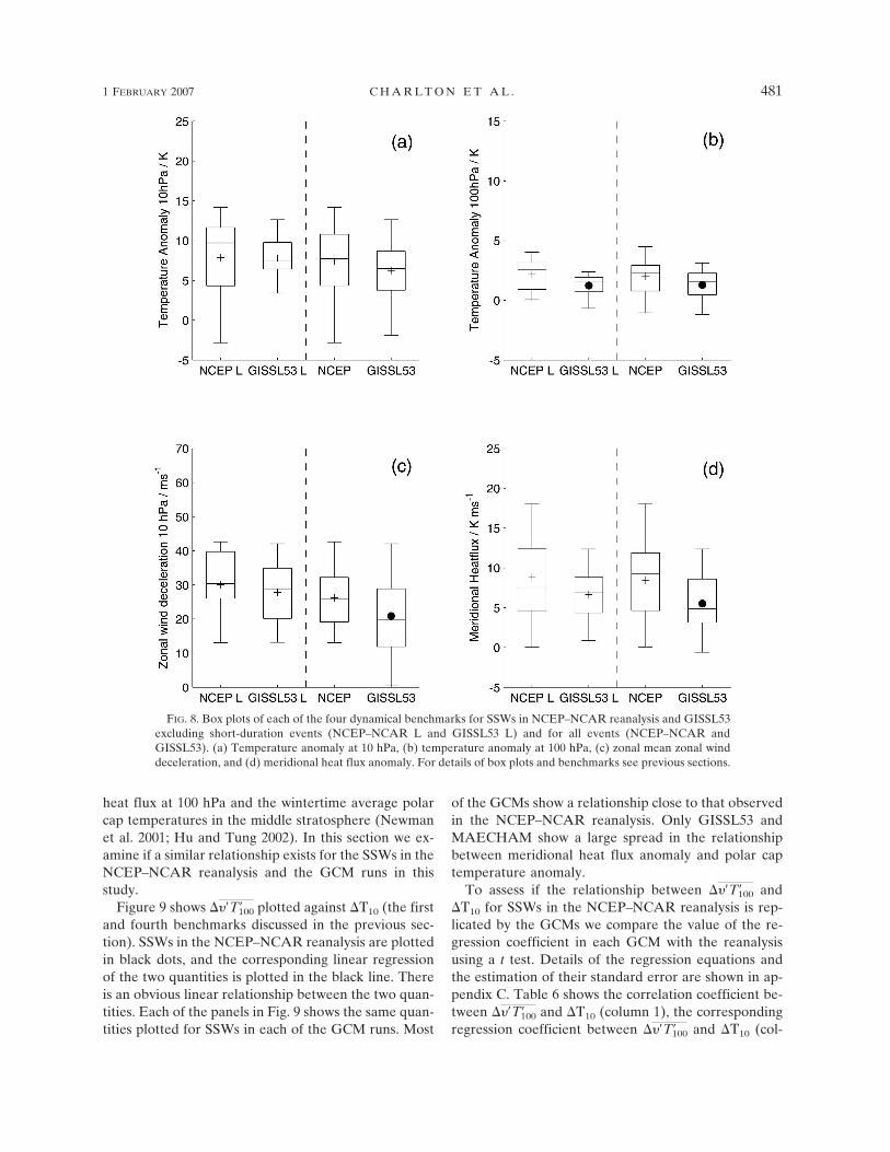
Table 5 shows the number of SSWs in each GCM withduration less than 4 days (column 2) and 4–9 days (col-umn 3), and with duration longer than 9 days (column4). The distribution of events in each category can becompared with the NCEP–NCAR reanalysis using an2 test (appendix B); the results of this test at the 0.05confidence level are shown in column 5. The mean du-ration of SSWs in each GCM is shown in column 6.

Table 5 shows that GISSL53 and MAECHAM havea significantly different distribution of SSW durationthan the NCEP–NCAR reanalysis. GISSL53 has ahigher proportion of short duration events than theNCEP–NCAR reanalysis (and also a distinct lack ofevents of the 4–9-day length). The majority of theseshort duration SSWs occur during February (9 of 20) inGISSL53, whereas they are fairly evenly distributed inthe NCEP–NCAR reanalysis. The GISSL53 model hasan unusually weak mean stratospheric vortex strengthduring February, which might be related to frequentSSWs in this month (Fig. 1).

To test if the high proportion of short duration (lessthan 4 days) SSWs in GISSL53 biases the distributionof benchmarks and distorts the results in the previoussection, all of the benchmarks are recomputed, exclud-ing events in the short event category. Figure 8 com-pares each of the dynamical benchmarks in the NCEP–NCAR reanalysis and GISSL53 models with and with-out short-duration SSWs. For both U10 and ��T�100,the difference between the mean benchmark for theNCEP–NCAR reanalysis and GISSL53 is reducedwhen short events are excluded. We conclude that theshort duration events, which are unusually prevalent inGISSL53, bias the benchmark diagnostics in the previ-ous section.

6. Discussion

From the previous two sections we have arrived attwo different but not contradictory conclusions aboutSSWs in the GCMs described here. First, in section 4we showed that three of the six GCM simulations of thewinter stratosphere produce a smaller number of SSWsthan are observed in reanalysis datasets. Second, weshowed in section 5 that the GCMs in the present studyproduce SSWs whose characteristics are statisticallysimilar to SSWs observed in the NCEP–NCAR re-analysis. This suggests that the lack of SSWs observedin section 4 is not due to an inability of the GCMs toreproduce the dynamics of SSW events but that thedynamics are produced less frequently than in the re-analysis dataset.

With this in mind, in this section we attempt to rec-oncile these two results by asking a number of ques-tions of the GCM simulations, designed to try andunderstand some of the reasons for the low frequencyof SSWs simulated by GISSL23, WACCM, andMRIJMA.

a. Is the relationship between ��T�100 and T10

correct in the GCMs?

Previous studies have shown that there is a good re-lationship between the wintertime average meridional

TABLE 5. Duration of SSWs in each GCM.

ModelShort events

�4 daysNormal events

4–9 daysLong events

�9 daysSignificant diff

NCEP–NCAR at 0.05Mean

duration/days

FVGCM 6 (26.1%) 10 (43.5%) 7 (30.4%) No 7.2GISSL53 20 (54.1%) 7 (18.9%) 10 (27.0%) Yes 6.1GISSL23 5 (41.7%) 5 (41.7%) 2 (16.7%) No 5.4WACCM 2 (40.0%) 1 (20.0%) 2 (40.0%) No 8.2MAECHAM 3 (20.0%) 2 (13.3%) 10 (66.7%) Yes 11.8MRIJMA 4 (28.6%) 6 (42.9%) 4 (28.6%) No 8.0NCEP–NCAR 12 (44.5%) 13 (48.1%) 2 (7.4%) 5.2

FIG. 7. Same as in Fig. 5, but for mean meridional heat fluxanomaly (75°–45°N) �20 to 0 days prior to SSWs.


heat flux at 100 hPa and the wintertime average polarcap temperatures in the middle stratosphere (Newmanet al. 2001; Hu and Tung 2002). In this section we ex-amine if a similar relationship exists for the SSWs in theNCEP–NCAR reanalysis and the GCM runs in thisstudy.

Figure 9 shows ��T�100 plotted against �10 (the firstand fourth benchmarks discussed in the previous sec-tion). SSWs in the NCEP–NCAR reanalysis are plottedin black dots, and the corresponding linear regressionof the two quantities is plotted in the black line. Thereis an obvious linear relationship between the two quan-tities. Each of the panels in Fig. 9 shows the same quan-tities plotted for SSWs in each of the GCM runs. Most

of the GCMs show a relationship close to that observedin the NCEP–NCAR reanalysis. Only GISSL53 andMAECHAM show a large spread in the relationshipbetween meridional heat flux anomaly and polar captemperature anomaly.

To assess if the relationship between ��T�100 and�10 for SSWs in the NCEP–NCAR reanalysis is rep-licated by the GCMs we compare the value of the re-gression coefficient in each GCM with the reanalysisusing a t test. Details of the regression equations andthe estimation of their standard error are shown in ap-pendix C. Table 6 shows the correlation coefficient be-tween ��T�100 and �10 (column 1), the correspondingregression coefficient between ��T�100 and �10 (col-

FIG. 8. Box plots of each of the four dynamical benchmarks for SSWs in NCEP–NCAR reanalysis and GISSL53excluding short-duration events (NCEP–NCAR L and GISSL53 L) and for all events (NCEP–NCAR andGISSL53). (a) Temperature anomaly at 10 hPa, (b) temperature anomaly at 100 hPa, (c) zonal mean zonal winddeceleration, and (d) meridional heat flux anomaly. For details of box plots and benchmarks see previous sections.


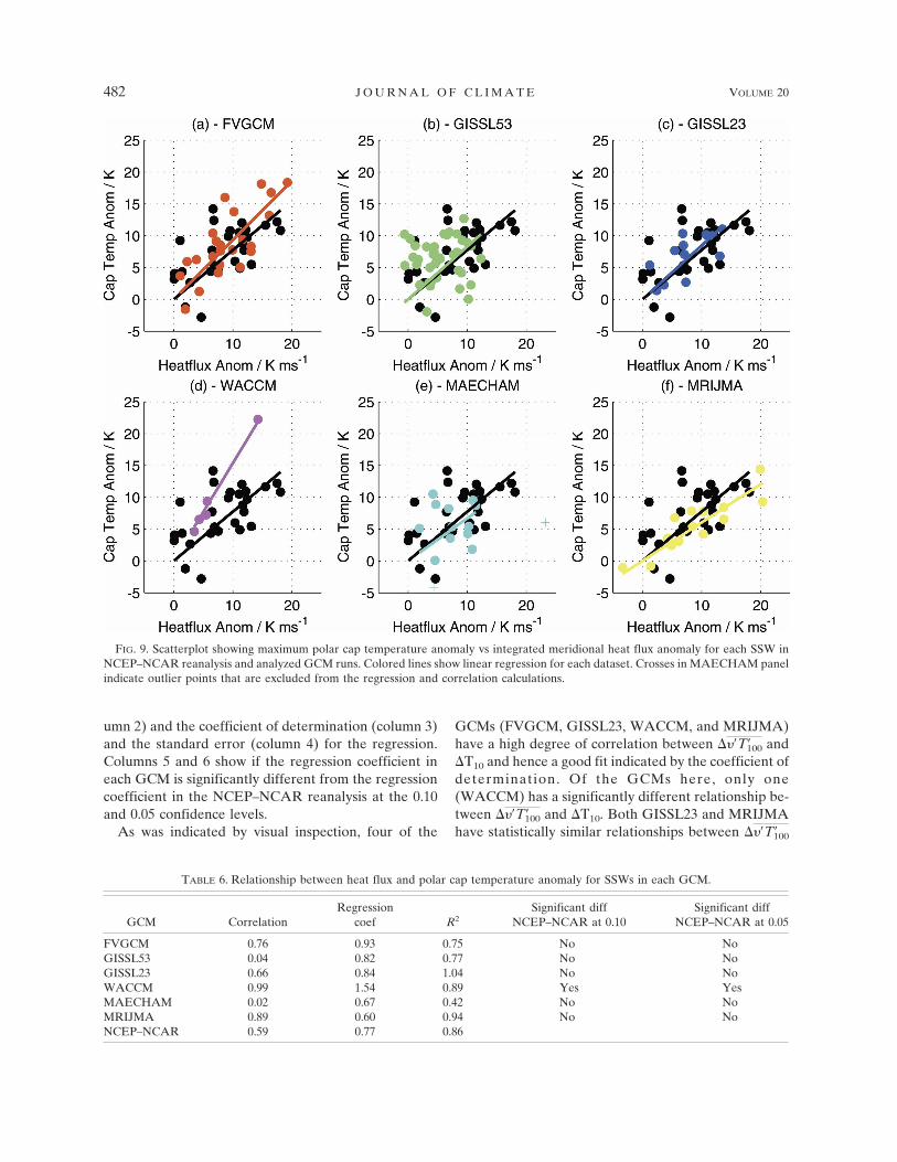
umn 2) and the coefficient of determination (column 3)and the standard error (column 4) for the regression.Columns 5 and 6 show if the regression coefficient ineach GCM is significantly different from the regressioncoefficient in the NCEP–NCAR reanalysis at the 0.10and 0.05 confidence levels.

As was indicated by visual inspection, four of the

GCMs (FVGCM, GISSL23, WACCM, and MRIJMA)have a high degree of correlation between ��T�100 and�10 and hence a good fit indicated by the coefficient ofdetermination. Of the GCMs here, only one(WACCM) has a significantly different relationship be-tween ��T�100 and �10. Both GISSL23 and MRIJMAhave statistically similar relationships between ��T�100

TABLE 6. Relationship between heat flux and polar cap temperature anomaly for SSWs in each GCM.

GCM CorrelationRegression

coef R2Significant diff

NCEP–NCAR at 0.10Significant diff

NCEP–NCAR at 0.05

FVGCM 0.76 0.93 0.75 No NoGISSL53 0.04 0.82 0.77 No NoGISSL23 0.66 0.84 1.04 No NoWACCM 0.99 1.54 0.89 Yes YesMAECHAM 0.02 0.67 0.42 No NoMRIJMA 0.89 0.60 0.94 No NoNCEP–NCAR 0.59 0.77 0.86

FIG. 9. Scatterplot showing maximum polar cap temperature anomaly vs integrated meridional heat flux anomaly for each SSW inNCEP–NCAR reanalysis and analyzed GCM runs. Colored lines show linear regression for each dataset. Crosses in MAECHAM panelindicate outlier points that are excluded from the regression and correlation calculations.


Fig 9 live 4/C

and T10 as the NCEP–NCAR reanalysis, suggestingthat a weak response of the stratosphere to meridionalheat flux anomalies is not the cause of the significantlack of warmings in either model.

There are however some caveats to these results; asnoted before, the sample size of the WACCM diagnos-tic is relatively small. It is also difficult to have muchconfidence in the MAECHAM and GISSL53 results,given that the correlation between ��T�100 and T10 inthese GCMs is very small. The correlation between��T�100 and T10 increases to 0.29 for GISSL53 whenevents of short duration (less than 4 days) are excludedand to 0.20 for MAECHAM when events of long du-ration (more than 9 days) are excluded. These correla-tions are still much less than the equivalent for theNCEP–NCAR reanalysis.

b. Do the GCMs simulate the correct number ofdays of extreme ��T�100?

Another reason for the lack of SSW activity in someof the GCMs, might be that the frequency of extreme

meridional heat flux anomalies, which tend to precedeSSWs as seen in the previous section, is lower than thatof the reanalysis data. To assess this we count the num-ber of days with extreme meridional heat flux anoma-lies in each GCM. For each winter season [November–March (NDJFM)] the number of days with a meanarea-weighted meridional heat flux anomaly greaterthan 8.5 K m s�1 [the mean value of ��T�100 for SSWsin the NCEP–NCAR reanalysis (cf. Fig. 7)] is calculated.

Figure 10 shows histograms for each of the GCMs ingray bars and for the NCEP–NCAR reanalysis in theclear bars. Only the two GISS GCMs have distributionswith a noticeable lack of extreme heat flux anomaliescompared to the reanalysis. This is particularly true ofGISSL23; GISSL23 also has a mean heat flux muchsmaller than the reanalysis data, indicating that it has adistinct lack of large absolute heat flux as expected.Two of the GCMs that have a significant lack of SSWactivity (WACCM and MRIJMA) have distributionsindicating a higher frequency of extreme heat flux daysthan the reanalysis.

FIG. 10. Histogram showing number of days of heat flux anomaly greater than 8.5 K m s�1 in NDJFM each winter. Gray bars showeach GCM; white bars show NCEP–NCAR reanalysis.


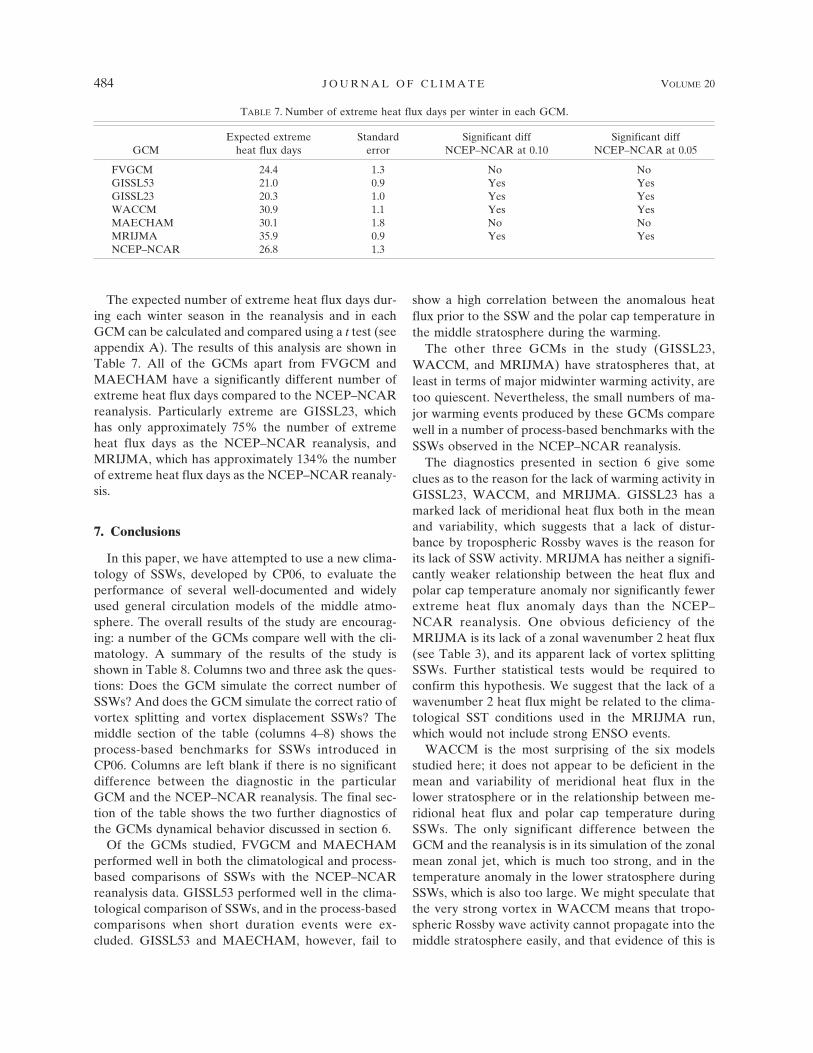
The expected number of extreme heat flux days dur-ing each winter season in the reanalysis and in eachGCM can be calculated and compared using a t test (seeappendix A). The results of this analysis are shown inTable 7. All of the GCMs apart from FVGCM andMAECHAM have a significantly different number ofextreme heat flux days compared to the NCEP–NCARreanalysis. Particularly extreme are GISSL23, whichhas only approximately 75% the number of extremeheat flux days as the NCEP–NCAR reanalysis, andMRIJMA, which has approximately 134% the numberof extreme heat flux days as the NCEP–NCAR reanaly-sis.

7. Conclusions

In this paper, we have attempted to use a new clima-tology of SSWs, developed by CP06, to evaluate theperformance of several well-documented and widelyused general circulation models of the middle atmo-sphere. The overall results of the study are encourag-ing: a number of the GCMs compare well with the cli-matology. A summary of the results of the study isshown in Table 8. Columns two and three ask the ques-tions: Does the GCM simulate the correct number ofSSWs? And does the GCM simulate the correct ratio ofvortex splitting and vortex displacement SSWs? Themiddle section of the table (columns 4–8) shows theprocess-based benchmarks for SSWs introduced inCP06. Columns are left blank if there is no significantdifference between the diagnostic in the particularGCM and the NCEP–NCAR reanalysis. The final sec-tion of the table shows the two further diagnostics ofthe GCMs dynamical behavior discussed in section 6.

Of the GCMs studied, FVGCM and MAECHAMperformed well in both the climatological and process-based comparisons of SSWs with the NCEP–NCARreanalysis data. GISSL53 performed well in the clima-tological comparison of SSWs, and in the process-basedcomparisons when short duration events were ex-cluded. GISSL53 and MAECHAM, however, fail to

show a high correlation between the anomalous heatflux prior to the SSW and the polar cap temperature inthe middle stratosphere during the warming.

The other three GCMs in the study (GISSL23,WACCM, and MRIJMA) have stratospheres that, atleast in terms of major midwinter warming activity, aretoo quiescent. Nevertheless, the small numbers of ma-jor warming events produced by these GCMs comparewell in a number of process-based benchmarks with theSSWs observed in the NCEP–NCAR reanalysis.

The diagnostics presented in section 6 give someclues as to the reason for the lack of warming activity inGISSL23, WACCM, and MRIJMA. GISSL23 has amarked lack of meridional heat flux both in the meanand variability, which suggests that a lack of distur-bance by tropospheric Rossby waves is the reason forits lack of SSW activity. MRIJMA has neither a signifi-cantly weaker relationship between the heat flux andpolar cap temperature anomaly nor significantly fewerextreme heat flux anomaly days than the NCEP–NCAR reanalysis. One obvious deficiency of theMRIJMA is its lack of a zonal wavenumber 2 heat flux(see Table 3), and its apparent lack of vortex splittingSSWs. Further statistical tests would be required toconfirm this hypothesis. We suggest that the lack of awavenumber 2 heat flux might be related to the clima-tological SST conditions used in the MRIJMA run,which would not include strong ENSO events.

WACCM is the most surprising of the six modelsstudied here; it does not appear to be deficient in themean and variability of meridional heat flux in thelower stratosphere or in the relationship between me-ridional heat flux and polar cap temperature duringSSWs. The only significant difference between theGCM and the reanalysis is in its simulation of the zonalmean zonal jet, which is much too strong, and in thetemperature anomaly in the lower stratosphere duringSSWs, which is also too large. We might speculate thatthe very strong vortex in WACCM means that tropo-spheric Rossby wave activity cannot propagate into themiddle stratosphere easily, and that evidence of this is

TABLE 7. Number of extreme heat flux days per winter in each GCM.

GCMExpected extreme

heat flux daysStandard

errorSignificant diff

NCEP–NCAR at 0.10Significant diff

NCEP–NCAR at 0.05

FVGCM 24.4 1.3 No NoGISSL53 21.0 0.9 Yes YesGISSL23 20.3 1.0 Yes YesWACCM 30.9 1.1 Yes YesMAECHAM 30.1 1.8 No NoMRIJMA 35.9 0.9 Yes YesNCEP–NCAR 26.8 1.3


provided by the high lower-stratospheric temperatureduring the major warming. In other words, much of themomentum deposition from planetary wave activity inWACCM may occur below the 10-hPa pressure surfacewhere we have defined SSWs. It should be kept in mindhowever that the interpretation of the WACCM resultsrequires some caution because of the small number ofSSWs found in the simulation studied.

Finally, there appears to be some relationship be-tween the strength of the climatological vortex in themiddle stratosphere and the number of SSWs. In CP06we showed that SSWs make little impact on wintertimemean polar cap temperatures (CP06, their Fig. 5). It istherefore appropriate to conclude that the climatologyis largely unaffected by the frequency of SSWs. On theother hand, in the present study we have found thatthose GCMs with a strong climatological vortex alsotend to have a lower frequency of SSWs than the re-analysis, and those GCMs with a weak climatologicalvortex also tend to have higher-frequency SSWs thanthe reanalysis. Thus, the strength of the climatologicalvortex might be a useful guide to the ability of GCMs toproduce the observed frequency of SSWs.

One of the key difficulties in reproducing the ob-served climatological vortex is the tuning of the gravitywave parameterization (GWP) in stratosphere-resolv-ing GCMs, and in particular the gravity wave momen-tum deposition in the mesosphere (Manzini and Mc-Farlane 1998). The effect of tuning the GWP on SSWfrequency has been little studied, although there issome evidence that the variability of the stratospheremay be insensitive to changes to the GWP (Chris-tiansen 1999), and this would be an interesting exten-sion to this paper when and if appropriate runs with asingle GCM and a variety of GWP setups becomesavailable. We hope that the climatological and process-based benchmarks for the simulation of SSWs intro-duced in this study will provide an additional constraintthat will prove useful to modelers wishing to tunestratosphere-resolving GCMs. In this study we also re-stricted our analysis to major SSWs (as defined byCP06); it might be interesting and useful in the future to

investigate the more frequent minor warming activitypresent in GCMs and reanalysis.

The study shows that making comparisons betweenGCMs and their simulation of major warming activity isboth useful and illuminating. Analyzing the variabilityof the northern winter stratosphere is important to un-derstanding northern polar ozone chemistry, futurechanges to northern winter climate, and the impact ofthese changes on the troposphere. This study showsthat certain stratosphere-resolving GCMs might not besuitable for analyzing these three important issues,given that they fail to simulate observed stratosphericvariability successfully. While no common solution tothe deficiencies identified in the GCMs immediatelyarises, there is nonetheless a great deal of progress thatcan be made by considering very simple diagnostics.

Acknowledgments. AJC and LMP were funded by anaward to the Cooperative Institute for Climate Appli-cations and Research (CICAR) from the U.S. NationalOceanic and Atmospheric Administration and by agrant to Columbia University from the U.S. NationalScience Foundation. JP’s research is funded by theNASA Climate Program Office. NCEP–NCAR re-analysis data were obtained from the Ingrid data serverat Columbia University. We thank Jeff Jonas and Pat-rick Lonergan for carrying out the GISSL53 andGISSL23 runs, respectively. The paper greatly ben-efited from discussion with Darryn Waugh, Gavin Es-ler, and Matthew Wittman.

APPENDIX A

Statistical Test of SSW Frequency

To compare the frequency of SSWs in each GCM runwith the frequency of SSWs in the reanalysis data weconsider each winter in the reanalysis or model run tobe a separate, independent observation of the fre-quency of major warming events per winter. Thus, forexample, in the NCEP–NCAR dataset we have 45 ob-servations of the frequency of events per winter, 23

TABLE 8. Summary of characteristics of each GCM.

GCM Frequency Type T10 T100 U10 ��T�100

Heat flux vscap temperature

Extremeheat flux

FVGCM Yes Yes LargeGISSL53 Yes No Small SmallGISSL23 No No Large SmallWACCM No Yes Large Large LargeMAECHAM Yes YesMRIJMA No Yes Large Large


observations with no events, 17 with one event, and 5with two events. The sample mean frequency (x) ofSSWs per winter season is the expected value of the 45observations in the NCEP–NCAR reanalysis:

x � E X � � �x

xPr{X � x}. �A1�

In Eq. (A1) x represents an observed frequency ofSSWs per winter and Pr{X � x} is the probability withwhich that frequency is observed. The sample varianceof the frequency of warming events s2 is calculated in asimilar fashion using

s2 � �x

�x � x�2Pr{X � x}. �A2�

The sample variance and the number of SSWs in eachdataset N are used to estimate the sample standarderror e of the expected mean frequency of SSWs:

e ��s2

�N. �A3�

The values of x and e are used to construct a t test thatcompares the mean frequency of SSWs in the reanalysisand a given GCM. The null hypothesis of this test is asfollows: The mean frequency of SSWs in the GCM andNCEP–NCAR reanalysis is equal. The test is two-sidedbecause there is no a priori reason to expect that thedifference between the means should be positive ornegative. A t statistic comparing the expected fre-quency of each model run and the NCEP–NCAR re-analysis is calculated in the standard way (Wilks 1995,p. 122):

t �xr � xm

er2 � em

2 �1�2 . �A4�

The r subscript denotes reanalysis statistics and the msubscript denotes model statistics. The t statistic is thencompared to critical values of a t distribution with de-grees of freedom calculated using the expression,

df ��er

2 � em2 �2

�er2�2��Nr � 1� � �em

2 �2��Nm � 1�. �A5�

APPENDIX B

Statistical Test of SSW Type

To test if each GCM has a similar proportion of vor-tex displacements and splits we construct a nonpara-metric 2 test. The null hypothesis of this test is asfollows: The frequency distributions of vortex displace-ment and splitting events in the GCM and NCEP–NCAR reanalysis are the same. First, a table is con-

structed showing the number of vortex displacementsand splits in the GCM and the NCEP–NCAR reanaly-sis. For example, for the FVGCM model the tablereads,

Vortex displacements Vortex splits

FVGCM 13 10NCEP–NCAR 15 12

Second the expected number of observations, Eij foreach cell is calculated, where i is the row index and j isthe column index. Under the null hypothesis that thesamples are drawn from the same distribution,

Eij � � �j�1

J

Oij

�i�1

I

�j�1

J

Oij��i�1

I

Oij, �B1�

where Oij is the observed number of SSWs in each boxof the table, I is the total number of columns, and J isthe total number of rows. The expected frequencies forTable B1 are

Vortex displacements Vortex splits

FVGCM 12.88 10.12NCEP–NCAR 15.12 11.88

The 2 parameter is estimated using the equation,

�2 � �i�1

I

�j�1

J�Oij � Eij�

2

Eij. �B2�

For the FVGCM example 2 � 0.0047. The value of 2

can then be compared to critical values of the 2 distri-bution with one degree of freedom. Critical values atthe 0.10 and 0.05 confidence levels are 2.7060 and3.8410, respectively. In the FVGCM example, the 2

value is well below the critical values so we cannotreject the null hypothesis that the frequency distribu-tions of vortex displacement and splitting events inFVGCM and the NCEP–NCAR reanalysis are thesame.

APPENDIX C

Statistical Test of Regression Parameters

For SSWs in both the GCM runs and the NCEP–NCAR reanalysis the regression model is as follows:

yi � �xi � ei, �C1�

where y represents T10, x represents ��T�100, ei repre-sents normally distributed residuals, and � is the pa-rameter of the model to be determined. No constant


term is included in the regression equation, because it isassumed that when ��T�100 is equal to zero T10 is alsoequal to zero. The value of � is estimated using theequation

� �

�i�1

N

yixi

�i�1

N

xi2

. �C2�

The sum of the squared residuals is calculated from theequation

r � �i�1

N

�yi � �xi�2. �C3�

The sum of the squared residuals is used to give anunbiased estimate of the residual variance, s2 � r/(n � 1).The standard error of the slope parameter is defined by

e �s

�i�1

N

xi2�1�2

. �C4�

As in appendix A, a t test is constructed using Eqs. (A3)and (A4) to compare the slope parameter of eachmodel and the NCEP–NCAR reanalysis. The null hy-pothesis of this test is as follows: The regression param-eter � is the same for SSWs in the model and the NCEP–NCAR reanalysis.

REFERENCES

Andrews, D. G., J. R. Holton, and C. B. Leovy, 1985: Middle At-mosphere Dynamics. Academic Press, 489 pp.

Austin, J., and Coauthors, 2003: Uncertainties and assesments ofchemistry-climate models of the stratosphere. Atmos. Chem.Phys., 3, 1–27.

Bloom, S., and Coauthors, 2005: Documentation and validation ofthe Goddard Earth Observing Ststem (GEOS) Data Assimi-lation System—Version 4. Technical Report Series on GlobalModelling and Data Assimilation, Tech. Rep. 26, 187 pp.

Butchart, N., J. Austin, J. R. Knight, A. A. Scaife, and M. L. Gal-lani, 2000: The response of the stratospheric climate to pro-jected changes in the concentrations of well-mixed green-house gases from 1992 to 2051. J. Climate, 13, 2142–2159.

Charlton, A. J., and L. M. Polvani, 2007: A new look at strato-spheric sudden warmings. Part I: Climatology and modelingbenchmarks. J. Climate, 20, 449–469.

Chiba, M., K. Yamazaki, K. Shibata, and Y. Kuroda, 1996: Thedescription of the MRI atmospheric spectral GCM (MRI-GSPM) and its mean statistics based on a 10-year integration.Papers Meteor. Geophys., 47, 1–45.

Christiansen, B., 1999: Stratospheric vacillations in a general cir-culation model. J. Atmos. Sci., 56, 1858–1872.

Erlebach, P., U. Langematz, and S. Pawson, 1995: Simulations ofstratospheric sudden warmings in the Berlin troposphere-stratosphere-mesosphere GCM. Ann. Geophys., 14, 443–463.

Eyring, V., and Coauthors, 2005: A strategy for process-orientedvalidation of coupled chemistry–climate models. Bull. Amer.Meteor. Soc., 86, 1117–1133.

Fortuin, J. P. F., and H. Kelder, 1998: An ozone climatology basedon ozonesonde and satellite measurements. J. Geophys. Res.,103, 31 709–31 734.

Gates, W. L., and Coauthors, 1999: An overview of the results ofthe Atmospheric Model Intercomparison Project (AMIP I).Bull. Amer. Meteor. Soc., 80, 29–55.

Hansen, J., G. Russell, D. Rind, P. Stone, A. Lacis, S. Lebedeff, R.Ruedy, and L. Travis, 1983: Efficient three-dimensional glob-al models for climate studies: Models I and II. Mon. Wea.Rev., 111, 609–662.

Hartmann, D. L., J. M. Wallace, V. Limpasuvan, D. W. J. Thomp-son, and J. R. Holton, 2000: Can ozone depletion and globalwarming interact to produce rapid climate change? Proc.Natl. Acad. Sci. USA, 97, 1412–1417.

Hu, Y., and K. K. Tung, 2002: Interannual and decadal variationsof planetary wave activity, stratospheric cooling, and North-ern Hemisphere Annular Mode. J. Climate, 15, 1659–1673.

JMA, 1997: Outline of the operational numerical weather predic-tion at the Japan Meteorological Agency. Japan Meteoro-logical Agency, 120 pp.

Kallberg, P., A. Simmons, S. Uppala, and M. Fuentes, 2004:The ERA-40 archive. ERA-40 Project Report Series, No. 17,ECMWF, 31 pp.

Kiehl, J. T., J. J. Hack, G. B. Bonan, B. A. Boville, D. L. William-son, and P. J. Rasch, 1998: The National Center for Atmo-spheric Research Community Climate Model: CCM3. J. Cli-mate, 11, 1151–1178.

Kistler, R., and Coauthors, 2001: The NCEP–NCAR 50-Year Re-analysis: Monthly means CD-ROM and documentation. Bull.Amer. Meteor. Soc., 82, 247–267.

Langematz, U., 2000: An estimate of the impact of observedozone losses on stratospheric temperature. Geophys. Res.Lett., 27, 2077–2080.

Liang, X. Z., W. C. Wang, and J. S. Boyle, 1997: Atmosphericozone climatology for use in general circulation models.Tech. Rep. 43, PCMDI, 25 pp.

Lin, S.-J., 2004: A “vertically Langrangian” finite-volume dynami-cal core for global models. Mon. Wea. Rev., 132, 2293–2307.

London, J., R. D. Bojkov, S. Oltmans, and J. I. Kelley, 1976: Atlasof the global distribution of total ozone. NCAR Tech. Note113, 276 pp.

Manzini, E., and L. Bengtsson, 1996: Stratospheric climate andvariability from a general circulation model and observations.Climate Dyn., 12, 615–639.

——, and N. A. McFarlane, 1998: The effect of varying the sourcespectrum of a gravity wave parameterization in a middle at-mosphere general circulation model. J. Geophys. Res., 103,31 523–31 539.

——, M. A. Giorgetta, M. Esch, L. Kornblueh, and E. Roeckner,2006: The influence of sea surface temperature on the north-ern winter stratosphere: Ensemble simulations with theMAECHAM5. J. Climate, 19, 3863–3881.

Newman, P. A., E. R. Nash, and J. E. Rosenfield, 2001: What con-trols the temperature of the Arctic stratosphere during thespring? J. Geophys. Res., 106, 19 999–20 010.

Pawson, S., and Coauthors, 2000: The GCM-Reality Intercom-parison Project for SPARC: Scientific issues and initial re-sults. Bull. Amer. Meteor. Soc., 81, 781–796.

Polvani, L. M., and D. W. Waugh, 2004: Upward wave activityflux as precursor to extreme stratospheric events and subse-


quent anomalous surface weather regimes. J. Climate, 17,3548–3554.

Rayner, N. A., D. E. Parker, E. B. Horton, C. K. Folland, L. V.Alexander, D. P. Rowell, E. Kent, and A. Kaplan, 2003:Global analyses of sea surface temperature, sea ice, andnighttime marine temperature since the late nineteenth cen-tury. J. Geophys. Res., 108, 4407, doi:10.1029/2002JD002670.

Rind, D., R. Suozzo, N. K. Balachandran, A. Lacis, and G. Rus-sell, 1988: The GISS Global Climate–Middle AtmosphereModel. Part I: Model structure and climatology. J. Atmos.Sci., 45, 329–370.

——, D. Shindell, P. Lonergan, and N. K. Balachandran, 1998:Climate change and the middle atmosphere. Part III: Thedoubled CO2 climate revisited. J. Climate, 11, 876–894.

——, J. Lerner, K. Shah, and R. Suozzo, 1999: Use of on-linetracers as a diagnostic tool in general circulation model de-velopment: 2. Transport between the troposphere and strato-sphere. J. Geophys. Res., 104, 9151–9167.

——, ——, J. Perlwitz, C. McLinden, and M. Prather, 2002: Sen-sitivity of tracer transports and stratospheric ozone to seasurface temperature patterns in the doubled CO2 climate. J.Geophys. Res., 107, 4800, doi:10.1029/2002JD002483.

Roeckner, E., and Coauthors, 2003: The atmospheric general cir-culation model ECHAM5, Part I: Model description. Tech.Rep. 349, MPI, Hamburg, Germany, 140 pp.

Sassi, F., R. R. Garcia, B. A. Boville, and R. Roble, 2004: Effect ofEl Niño–Southern Oscillation on the dynamical, thermal, andchemical structure of the middle atmosphere. J. Geophys.Res., 109, D17108, doi:10.1029/2003JD004434.

Schmidt, G. A., and Coauthors, 2006: Present-day atmosphericsimulations using GISS ModelE: Comparisons to in situ, sat-ellite, and reanalysis data. J. Climate, 19, 153–192.

Schnadt, C., and M. Dameris, 2003: Relationship between NorthAtlantic Oscillation changes and stratospheric ozone recov-ery in the Northern Hemisphere in a chemistry-climatemodel. Geophys. Res. Lett., 30, 1487, doi:10.1029/2003GL017006.

Shibata, K., H. Yoshimura, M. Ohizumi, M. Hosaka, and M. Sugi,1999: A simulation of troposphere, stratosphere and meso-sphere with an MRI/JMA98 GCM. Papers Meteor. Geophys.,50, 15–53

Shindell, D. T., D. Rind, and P. Lonergan, 1998: Increased polarstratospheric ozone losses and delayed eventual recovery ow-ing to increased greenhouse gas concentrations. Nature, 392,589–592.

——, R. L. Miller, G. A. Schmidt, and L. Pandolfo, 1999: Simu-lation of recent northern winter climate trends by greenhousegas forcing. Nature, 399, 452–455.

Shine, K. P., and Coauthors, 2003: A comparison of model-simulated trends in stratospheric temperatures. Quart. J. Roy.Meteor. Soc., 129, 1565–1588.

Stolarski, R. S., A. R. Douglass, S. Steenrod, and S. Pawson, 2005:Trends in stratospheric ozone: Lessons learned from a 3Dchemical transport model. J. Atmos. Sci., 63, 1028–1041.

Wilks, D. S., 1995: Statistical Methods in the Atmospheric Sciences.Academic Press, 648 pp.


Documents

A New Look at Stratospheric Sudden Warmings. Part II