A New Group Contribution Method For The … New Group Contribution Method for the Estimation of Thermal Conductivity of Non-Electrolyte Organic Compounds By Onellan Govender [B.Sc

A New Group Contribution Method for the

Estimation of Thermal Conductivity of

Non-Electrolyte Organic Compounds

By

Onellan Govender [B.Sc. (Eng.)]

University of KwaZulu-Natal Durban

In fulfilment of the degree Master of Science (Chemical Engineering)

2011

Examiner’s Copy

Abstract

The optimum design of heat and mass transfer equipment forms an integral part of cost-effective plant

design. For this purpose, reasonably accurate thermal conductivity data are required for all phases.

Modern reliable equipment is now available for the routine measurement of liquid thermal

conductivity but due to the large amount of data needed and costs of experiments, alternative sources

such as predictive methods are often employed. Substantial effort has been invested into the

development of models for prediction and correlation of liquid thermal conductivity. Prediction of

liquid thermal conductivity based solely on a theoretical basis does not provide reliable results as the

theories used to describe the liquid state are seldom satisfactory (Rodenbush et al., 1999). Therefore,

prediction of thermo-physical properties is most often based upon empirical approaches like group

contribution methods.

Methods for the estimation of the normal boiling point (Cordes and Rarey, 2002, Nannoolal et al.,

2004), critical property data (Nannoolal et al., 2007), vapour pressures (Moller et al., 2008, Nannoolal

et al., 2008) and liquid viscosity (Nannoolal et al., 2009) have previously been developed in our group

using the group contribution approach. Based on these methods a more accurate and precise method

with a better temperature dependency is presented for liquid thermal conductivity prediction. The data

used to develop the method was obtained from the extensive Dortmund Data Bank (DDB) (Gmehling

et al., 2009), which contains approximately 110000 pure component thermal conductivity data points

for almost 900 different compounds for the various phases. Only a third of the components and even

fewer data points were usable after critical evaluation; however, the model still has a wider range of

applicability than previous correlations and models, which were based on smaller experimental data

sets.

The relative mean deviation (RMD) for the training set was found to be 3.87 % (331 compounds and

6264 data points). Applicability to data outside the training and performance of the model was tested

using an external set of liquid thermal conductivity data. The RMD for the test set was 7.68 % for 38

compounds (328 data points). This error was found to be high as the test set contained data

extrapolated from experimental data at elevated pressures, and other less reliable data which was

excluded from the training set. The results from the test set show that the method may be applied to

components outside the training set with reasonable confidence.

Preface

The work presented in this dissertation was undertaken at the University of KwaZulu-Natal Durban

from February 2009 until November 2011 and was supervised by Professor Dr. D. Ramjugernath and

Professor Dr. J. Rarey.

I Onellan Govender declare that:

(i) The research reported in this dissertation/thesis, except where otherwise indicated, is my

original work.

(ii) This dissertation has not been submitted for any degree or examination at any other

university.

(iii) This dissertation does not contain other persons’ data, pictures, graphs or other

information, unless specifically acknowledged as being sourced from other persons.

(iv) This dissertation does not contain other persons’ writing, unless specifically

acknowledged as being sourced from other researchers. Where other written sources have

been quoted, then:

a) their words have been re-written but the general information attributed to them has

been referenced;

b) where their exact words have been used, their writing has been placed inside quotation

marks, and referenced.

(v) Where I have reproduced a publication of which I am an author, co-author or editor, I

have indicated in detail which part of the publication was actually written by myself alone

and have fully referenced such publications.

(vi) This dissertation does not contain text, graphics or tables copied and pasted from the

Internet, unless specifically acknowledged, and the source being detailed in the

dissertation and in the References sections.

Signed:

____________________________

Onellan Govender (205502080)

As the candidate’s Supervisor I agree/do not agree to the submission of this thesis.

___________________________

Prof. Dr. D. Ramjugernath

Acknowledgements

This dissertation would not have been a real fulfilment without the backing and cooperation from the

following people and organizations for their contributions:

I am indebted to my supervisors, Prof. Dr. J. Rarey and Prof. Dr. D. Ramjugernath for their

tireless support, ideas and motivation without which, it would not have been possible to

produce this dissertation.

Bruce Moller, for helping me to get started with my work and guiding me throughout the

process of undertaking my master’s degree.

Eugene Olivier, for all his help and co-operation throughout the duration of the work.

DST/NRF South African Research Chair’s Programme, NRF International Science Liaison,

NRF-Thuthuka Programme and BMBF (WTZ-Project) for financial support.

DDBST GmbH for providing data and software support for this project.

My parents, Nelendri and Gonnie, for their support, guidance, and motivation throughout my

studies at University. Without the sacrifices they have made, I would not be who I am and

where I am today.

My colleagues and friends, Crysanther, Shivaan, Alan, Brian, Kishan, Tyrin and Warren for

their invaluable knowledge and support.

i

Table of Contents

1. Introduction..................................... ................................................................................................... 1

2. Theory and Literature Review ............................................................................................................ 3

2.1. Introduction ............................................................................................................................. 3

2.2. State Variable Dependency ..................................................................................................... 3

2.3. Experimental Methods ............................................................................................................ 8

2.4. Data Correlation Models ......................................................................................................... 9

2.5. Predictive Models .................................................................................................................. 11

2.6. Group Contribution Methods ................................................................................................ 13

2.6.1. Robbins and Kingrea (1962) ......................................................................................... 13

2.6.2. Nagvekar and Daubert (1987) ....................................................................................... 14

2.6.3. Assael, Charitidou & Wakeham (1989) ........................................................................ 16

2.6.4. Sastri and Rao (1993) .................................................................................................... 18

2.6.5. Rodenbush, Viswanath & Hsieh (1999) ........................................................................ 20

2.6.6. Sastri and Rao (1999) .................................................................................................... 21

2.7. Corresponding State Methods ............................................................................................... 23

2.7.1. Ely and Hanley (1983) .................................................................................................. 23

2.8. Empirical Correlations .......................................................................................................... 25

2.8.1. Sato and Reidel (1977) .................................................................................................. 25

2.8.2. Lakshmi and Prasad (1992) ........................................................................................... 26

2.8.3. Mathias, Parekh and Miller (2002) ................................................................................ 27

2.9. Summary ............................................................................................................................... 29

3. Computation and Database Tools ................................................................................................. 31

3.1. Database ................................................................................................................................ 31

3.2. Data validation ...................................................................................................................... 31

3.3. Regression ............................................................................................................................. 36

3.3.1. Linear regression ........................................................................................................... 36

3.3.2. Weighted linear regression ............................................................................................ 37

ii

3.3.3. Fragmentation................................................................................................................ 39

3.4. Summary ............................................................................................................................... 40

4. Development of the model............. ................................................................................................. 41

4.1. Model Development .............................................................................................................. 41

4.2. The Group Contribution Concept .......................................................................................... 47

5. Results and Discussion ................................................................................................................... 53

5.1. Hydrocarbon Compounds ..................................................................................................... 54

5.1.1. Forcing Rules ................................................................................................................ 57

5.2. Oxygen compounds ............................................................................................................... 58

5.3. Halogen compounds .............................................................................................................. 61

5.3.1. Group 17 Trends ............................................................................................................ 63

5.4. Nitrogen compounds ............................................................................................................. 66

5.5. Other compounds .................................................................................................................. 68

5.6. Testing the method ................................................................................................................ 69

5.7. Final results ........................................................................................................................... 70

6. Conclusions .................................................................................................................................... 74

7. Recommendations .......................................................................................................................... 75

8. References ...................................................................................................................................... 76

Appendix A: Group Contribution Tables ................................................................................................. I

Appendix B: Sample Calculations .......................................................................................................... V

Appendix C: Example Calculation Using the Mathias et al. Model .................................................... XII

Appendix D: Data Validation and Regression Interfaces .................................................................. XIX

iii

List of Tables

Table 2.1: Relative mean deviations (RMD) of liquid thermal conductivity for selected compounds

using the Nagvekar and Daubert (1987) method (NP = Number of data points) .................................. 16

Table 2.2: Coefficients for use in Eqns. (2.15) to (2.18) (m3.mol

-1) (Assael et al., 1989) .................... 17


using the Sastri and Rao (1993) method (NP = Number of data points) ............................................... 19


using the Sastri and Rao (1999) method (NP = Number of data points) ............................................... 22


using the Sato and Reidel (1977) method (NP = Number of data points) ............................................. 26


using the Lakshmi and Prasad (1992) method (NP = Number of data points) ...................................... 27

Table 5.1: Relative mean deviation [%] of thermal conductivity estimation for the different families of

hydrocarbons for the different models used. ......................................................................................... 56

Table 5.2: Relative mean deviation [%] of liquid thermal conductivity prediction for hydrocarbon

compounds. The number in superscript is the number of data points used; the main number is the

RMD for the respective reduced temperature range. ............................................................................ 57

Table 5.3: Liquid thermal conductivity of hexane and 4 different oxygenated hexane compounds at

their normal boiling points (Gmehling et al., 2009) .............................................................................. 58


oxygenated compounds for the different models used. ......................................................................... 59

Table 5.5: Relative mean deviation (RMD) [%] of liquid thermal conductivity prediction for

oxygenated compounds. The number in superscript is the number of data points used; the main

number is the RMD for the respective reduced temperature range. ...................................................... 61


halogenated compounds and the different models used. ....................................................................... 62

Table 5.7: Relative mean deviation (RMD) [%] of liquid thermal conductivity prediction for

halogenated compounds. The number in superscript is the number of data points used; the main

number is the RMD for the respective reduced temperature range. ...................................................... 62

Table 5.8: Electronic configuration for the first four halogen atoms from the periodic group 17

(Chemistry, 2012) ................................................................................................................................ 64

iv


nitrogen compounds and the different models used. ............................................................................. 67

Table 5.10: Relative mean deviation (RMD) [%] of liquid thermal conductivity prediction for nitrogen

compounds. The number in superscript is the number of data points used; the main number is the

RMD for the respective reduced temperature range. ............................................................................ 67

Table 5.11: Relative mean deviation [%] of thermal conductivity estimation for all other organic

families and the different models used. ................................................................................................. 68

Table 5.12: Relative mean deviation [%] of thermal conductivity estimation for the test set data and

the different models used. ..................................................................................................................... 69

Table 5.13: Relative mean deviation [%] of thermal conductivity estimation for the test set data for

halogenated compounds and the different models used. ....................................................................... 70

Table 5.14: Relative mean deviation [%] of thermal conductivity estimation for the new method and

literature methods. ................................................................................................................................. 71

Table 5.15: Regression and prediction results for respective group contribution methods as reported in

literature and calculated for the training set for the new model ............................................................ 71

Table C-1: Relative mean deviation (RMD) of thermal conductivity prediction results for Mathias et

al. (Mathias et al., 2002) (NC = number of compounds) ................................................................. XVIII

Table C-2: Relative mean deviation (RMD) of thermal conductivity prediction results for Mathias et

al. (Mathias et al., 2002) (ND = number of data points) .................................................................. XVIII

v

List of Figures

Figure 2.1: Thermal conductivity vs. density for methane around the critical region (Tc = 190.6 K)

(Mathias et al., 2002) .............................................................................................................................. 4

Figure 2.2: Thermal conductivity vs. temperature for cyclopentane at 1atm (data from the DDB

(Gmehling et al., 2009)) .......................................................................................................................... 5

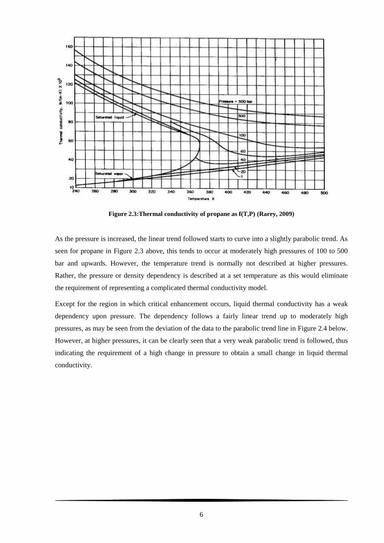
Figure 2.3:Thermal conductivity of propane as f(T,P) (Rarey, 2009) ..................................................... 6

Figure 2.4: Thermal conductivity vs. pressure for 1-octene at 320K (data from DDB (Gmehling et al.,

2009)) ...................................................................................................................................................... 7

Figure 2.5: Liquid thermal conductivity vs. density for 1-octene at 320K (♦ - exp. data from DDB

(Gmehling et al., 2009)) .......................................................................................................................... 7

Figure 2.6: Liquid thermal conductivity vs. temperature for tetra-ethylene-glycol (exp. data from DDB

(Gmehling et al., 2009)) .......................................................................................................................... 8

Figure 2.7: Liquid thermal conductivity vs. temperature for bromobenzene utilizing a linear trend for

correlation of data ( ■ – experimental data from DDB (Gmehling et al., 2009)) ................................. 10

Figure 2.8: Liquid thermal conductivity vs. temperature for bromobenzene utilizing a polynomial fit

for correlation of data ( ■ – experimental data from DDB (Gmehling et al., 2009)) ............................ 10

Figure 2.9: Liquid thermal conductivity vs. temperature for trichloroethylene (data from the DDB

(Gmehling et al., 2009)) ........................................................................................................................ 15


(Gmehling et al., 2009)) ........................................................................................................................ 19

Figure 2.11: Liquid thermal conductivity vs. temperature for cyclopentane (data from the DDB

(Gmehling et al., 2009)) ........................................................................................................................ 21


(Gmehling et al., 2009) ) ....................................................................................................................... 22

Figure 3.1: Liquid thermal conductivity vs. temperature for cyclohexane (1 atm (black) and elevated

pressures (green) – data from the DDB (Gmehling et al., 2009)) ......................................................... 32

Figure 3.2: Thermal conductivity of liquid toluene at 298.15 K (Rarey, 2009) .................................... 32

Figure 3.3: Vapour pressure curve for 1-octene (data from DDB (Gmehling et al., 2009)) ................. 34

Figure 3.4: Liquid thermal conductivity vs. pressure for 1-octene at 500K (data from DDB (Gmehling

et al., 2009)) .......................................................................................................................................... 34

Figure 3.5: Liquid thermal conductivity vs. temperature for cyclohexane (1atm - all data from DDB

(Gmehling et al., 2009)) ........................................................................................................................ 35

vi

Figure 3.6: Liquid thermal conductivity vs. temperature for cyclohexane showing the data used in the

training set (1atm – data from DDB (Gmehling et al., 2009)) .............................................................. 36

Figure 3.7: Liquid thermal conductivity vs. temperature for 1-pentanol (data from DDB (Gmehling et

al., 2009)) .............................................................................................................................................. 38

Figure 4.1: Liquid thermal conductivity vs. temperature for n-butane at 1atm [DDB (Gmehling et al.,

2009)] .................................................................................................................................................... 41

Figure 4.2: Slope of liquid thermal conductivity vs. temperature for ethylene glycols and its polymers

vs. number of carbon atoms for the high and low temperature sections ............................................... 42

Figure 4.3: Liquid thermal conductivity vs. temperature for diethylene glycol (data from DDB

(Gmehling et al., 2009)) ........................................................................................................................ 42

Figure 4.4: Liquid thermal conductivity vs. temperature for water (data from DDB (Gmehling et al.,

2009)) .................................................................................................................................................... 43

Figure 4.5: Liquid thermal conductivity vs. temperature for pentaethylene glycol (data from DDB

(Gmehling et al., 2009)) ........................................................................................................................ 43

Figure 4.6: Thermal conductivity (W.m-1

.K-1

) at the normal boiling point sorted into different bin

ranges (375 components) ...................................................................................................................... 46


.K-1

) at a standard temperature of 298 K sorted into different

bin ranges (149 components) ................................................................................................................ 46

Figure 4.8: Model slope (A) vs. number of carbon atoms for the n-alkane series ................................ 48

Figure 4.9: Model intercept (B) vs. number of carbon atoms for the n-alkane series displaying a non-

linear relationship .................................................................................................................................. 49

Figure 4.10: Linearized expression for model intercept (B) vs. number of carbon atoms for the n-

alkane series displaying the linearized relationship .............................................................................. 49

Figure 4.11: Model slope (A) and intercept (B) vs. number of carbon atoms for the n-alcohol series

without the size dependency term added ............................................................................................... 50

Figure 4.12: Error between model and group contribution predicted slope vs. number of carbon atoms

for the n-alcohol series .......................................................................................................................... 51


with the size dependency term added .................................................................................................... 52

Figure 5.1: Liquid thermal conductivity vs. temperature for heptane (Gmehling et al., 2009) ............ 53

Figure 5.2: Model slope (A) and intercept (B) vs. number of carbon atoms for the n-alkanes ............. 54

vii

Figure 5.3: Liquid thermal conductivity vs. temperature for tetradecane (data from the DDB

(Gmehling et al., 2009)) ........................................................................................................................ 55

Figure 5.4: Group contributions (∆A) for -CH3, >CH2, >CH- and >C< vs. their respective molecular

weight .................................................................................................................................................... 58

Figure 5.5: Liquid thermal conductivity vs. reduced temperature for 1,2-Ethanediol [Data obtained

from DDB (Gmehling et al., 2009)] ...................................................................................................... 60

Figure 5.6: Model intercept (B) contribution vs. respective atomic radii squared for a halogen attached

to a non-aromatic carbon (♦ - fitted group value) ................................................................................. 63

Figure 5.7: Pauling electronegativities vs. atomic radii for the halogen atoms..................................... 64

Figure 5.8: Model slope (A) contribution vs. respective atomic radii squared for a halogen attached to

a non-aromatic carbon (♦ - fitted group value, ◊ - new group value) .................................................... 65

Figure 5.9: Model intercept (B) contribution vs. respective atomic radii squared for a halogen attached

to an aromatic carbon (♦ - fitted group value) ....................................................................................... 65

Figure 5.10: Model slope (A) contribution vs. respective atomic radii squared for a halogen attached to

an aromatic carbon (♦ - fitted group value, ◊ - new group value) ......................................................... 66

Figure 5.11: Group contributions (∆A) for –NH2, >NH and >N- vs. their respective molecular weight

............................................................................................................................................................... 68

Figure 5.12: Histogram representing the relative mean deviation [%] distribution for the new method

compared to literature methods for training set data ............................................................................. 72


compared to literature methods for test set data .................................................................................... 72

Figure D-1: Initial data validation interface ....................................................................................... XIX

Figure D-2: Data validation interface including a correlation functions to validate trends ................. XX

Figure D-3: Structural parameter contribution regression interface ................................................... XXI

Figure D-4: Data validation interface utilizing correlation of high pressure data ............................. XXII

viii

Nomenclature

a, b, c, d, e - model parameters/constants

A, B, C, D, E - model parameters/constants

M - molar mass (g.mol-1

)

n - number of moles

P - pressure (kPa)

R - ideal gas constant (J.mol-1

.K-1

)

S - entropy (J.mol-1

.K-1

)

T - absolute temperature (K)

V - molar volume (cm3.mol

-1)

Z - compressibility factor

Greek symbols

λ - thermal conductivity (W.m-1

.K-1

)

μ - chemical potential

w - Pitzer acentric factor

Subscripts

b - normal boiling point

c - critical point

n - molar basis

r - reduced property

vap - vaporization

Superscripts

s - saturated / solid

l - liquid

v - vapour

__________________________________________

All other symbols used are explained in the text and unless otherwise stated SI units have been

used.

1

1. Introduction

The design of unit operations in industry is based upon the modelling of mass, momentum or heat

transfer for the different processes. This requires fairly accurate transport property data for the

evaluation of transfer coefficients and dimensionless numbers which are involved in the design of

equipment such as plug flow reactors, heat exchangers, flow meters, distillation columns, pumps, etc

(Nieto de Castro, 1990, Rodenbush et al., 1999). Optimum design of heat and mass transfer equipment

forms an integral part of cost-effective plant design.

In a study undertaken by Fujioka et al. for the design of a chemical heat pump to be used with a solid

catalyst bed reactor (Fujioka et al., 2006), a problem was encountered where a strongly exothermic

reaction formed products with low thermal conductivities. This prevented heat from being effectively

removed from the reaction. Research performed by the group indicated that an increase of the effective

heat transfer coefficient, up to a limit, could be used to decrease the reaction time down to a minimum.

Thus, design of the equipment could not be carried out without prior simulation of the equipment to

determine whether operation under the specific conditions was viable. In this design, the reaction rate

was controlled by process heat transfer; thus accurate transport data, thermal conductivity in particular

for heat transfer calculations, was required. The thermal conductivity for the reactants, products,

catalysts and reaction vessel can therefore play an important role in reactor design.

During the experimental determination of thermal conductivity of fluid phases, convective heat

transport has to be strictly avoided. Although modern reliable equipment is now available for the

routine measurement of liquid thermal conductivity, due to the large amount of data needed and the

costs of experiments, alternative sources such as predictive methods are often employed. Many

simulation packages such as ASPENTECH® or HYSYS

® use built in predictive methods to provide

physical, thermodynamic, and transport properties during process modelling and simulation.

There are many methods available for the prediction of thermal conductivity. However, many are

either complex or require the input of numerous other properties (Horvath, 1992). Routine prediction

of transport properties in an engineering context requires a method which is fast, simple to implement

and has minimum input requirements. Complex equations or the input requirement of a number of

properties may introduce errors into the calculation, which can then be difficult to trace when

introduced into a process simulation. To satisfy the aforementioned need, researchers have correlated

data using equations which require only inputs of either molecular mass, normal boiling point, or

correlated constants, together with the temperature for which to calculate or estimate the thermal

conductivity (Horvath, 1992, Lakshmi and Prasad, 1992, Poling et al., 2004).

It is for the above reasons that the group contribution concept has become increasingly popular for the

prediction of thermodynamic, thermophysical and transport properties. It is based on the principle that

the properties of a pure component can be predicted using only the structure of the molecule and the

state variables. In the group contribution method, the property of a pure compound is calculated from

2

the sum of the contributions of the structural groups (e.g. -CH2, -CHOOH, -C=C- etc.) of which it is

composed. The basic group contribution principle is based on the assumption that the effects of the

individual structural groups are additive (Moller, 2007). This additivity does not need to be with

respect to the property itself but may be for a general function of the property. This function usually

contains several empirical model parameters.

Seven group contribution methods and numerous empirical and semi-empirical correlations for liquid

thermal conductivity prediction have been found in literature. These methods provide a limited

temperature dependency and limited range of applicability. Prediction of liquid thermal conductivity

from molecular and kinetic theory often leads to unsatisfactory results as the theories used to describe

the liquid state are often insufficient (Rodenbush et al., 1999) to describe the energy transfer due to

collisions within the fluid.

Intermolecular forces govern the liquid behavior, and in some aspects, liquids more closely resemble a

solid than a gas. Therefore, utilising kinetic theory may work extremely well for the vapour phase, but

not for liquids.

Work done to date on group contribution method’s by the UKZN Thermodynamics Research Unit in

collaboration with the Carl von Ossietzky University includes the estimation of the normal boiling

point (Cordes and Rarey, 2002, Nannoolal et al., 2004), critical property data (Nannoolal et al., 2007),

vapour pressures (Moller et al., 2008, Nannoolal et al., 2008) and liquid viscosity (Nannoolal et al.,

2009).

This study aims to improve upon available thermal conductivity prediction methods with respect to the

range of applicability, temperature range within which the method is applicable, accuracy and

precision of prediction by implementation of the group contribution concept to a much larger

collection of thermal conductivity data than previously available. The tasks which were required for

the fulfilment of the aim are:

i. Undertaking a comprehensive review of all relevant literature;

ii. The compilation and critical evaluation of all the necessary experimental data to yield a

suitable data set (training set) which will be used for the regression of the structural

contributions;

iii. Development of a new empirical or semi-empirical model which would describe the

experimental data more accurately;

iv. Regression of the model parameters using the training set;

v. Regression of structural contributions based upon model parameters;

vi. Testing of the model using an independent set of experimental data (test set).

3

2. Theory and Literature Review

2.1. Introduction

It is well known that temperature gradients are the driving force for heat transfer either within or

between phases. Energy in the form of heat is always transferred from a region of high temperature to

one of low temperature. Conductive heat transfer occurs within a single phase (e.g. heat transfer

through a pipe wall) irrespective of the phase (gas, solid or liquid). Conductive heat transfer is given

mathematically by Fourier’s law as follows:

qJ (2.1)

In the above equation, λ is the thermal conductivity or transfer coefficient which relates Jq, the heat

flux and T , the temperature gradient (Assael et al., 1998). Thermal conductivity is therefore the

ability of a material to conduct heat or the degree to which the material can conduct heat. Assuming

that heat transfer occurs in one direction only and that the material is homogeneous (λ constant with

respect to x), Eqn. (2.1) may then be integrated producing the following analogous equation for one-

dimensional heat conduction:

q x T (2.2)

where ∆x is the shortest distance between two parallel layers inside the homogeneous phase and ∆T is

the temperature difference between these layers. If the temperature difference is constant with respect

to time then the heat flux is constant with respect to time and the following holds:

Q x

tA T

(2.3)

where ∆Q is the amount of heat transferred in the time interval ∆t through an area with cross section

A. In this equation, λ is a material constant that depends on temperature and pressure (density) and the

kind of material (pure component or mixture). Thermal conductivity may thus be described as the rate

at which heat transfer occurs within a system in a state of non-equilibrium (Assael et al., 1998).

2.2. State Variable Dependency

Any transport property, for example, thermal conductivity, may be written in terms of the state

variables temperature and density (density has a more linear relationship with thermal conductivity

than pressure as will be shown later on) as a function of three contributions as follows (Assael et al.,

1998):

4

( , ) ( ) ( , ) ( , )n o n c nT T T T (2.4)

The three contributions of Eqn. (2.4) represent the dilute-gas contribution (i.e. negligible pressure

effect), the excess contribution (pressure effect) and the critical enhancement contribution (Assael et

al., 1998). The sum of the first two contributions (dilute-gas and excess contribution) is called the

background contribution of the transport property. The background contribution represents the thermal

conductivity of the liquid sufficiently below the critical temperature and is the term most often

predicted for transport properties.

The background term, according to Ely and Hanley (Ely and Hanley, 1983), may be divided into two

different contributions as compared to those stated above. The first due to the transfer of energy from

solely collisional or translational effects, and the second resulting from the transfer of energy via the

internal degrees of freedom.

The divergence of transport properties at the critical point is known as “critical enhancement”. This

critical enhancement contribution may be described as the difference between the actual property at

the critical point and the extrapolated value of the property from lower temperatures or pressures.

When approaching the critical point, the mean free path of the molecules is in the order of the mean

distance between the particles and the differential

T

P

V approaches zero. In this way the stabilizing

effect of the pressure that usually provides homogeneity in density (or molar volume V) is lost and

strong fluctuations lead to strong increase of all transport phenomena. As shown in Figure 2.1, liquid

thermal conductivity shows strong enhancement around the critical region.

Figure 2.1: Thermal conductivity vs. density for methane around the critical region (Tc = 190.6 K)

(Mathias et al., 2002)

5

A review of available experimental data has indicated that there are large amounts of data measured at

high pressures (reduced pressures in the order of 5.5 to 200). There are however very few methods

available in literature which account for the pressure dependency.

Figure 2.2: Thermal conductivity vs. temperature for cyclopentane at 1atm (data from the DDB

(Gmehling et al., 2009))

For most organic liquids thermal conductivity has an inversely linear relationship with the state

property temperature at low pressures as shown in Figure 2.2. This relationship has been used many

times for the correlation of organic liquid thermal conductivity data (Horvath, 1992, Lakshmi and

Prasad, 1992, Nagvekar and Daubert, 1987, Reidel, 1951, Sastri and Rao, 1993, Sastri and Rao, 1999).

6

Figure 2.3:Thermal conductivity of propane as f(T,P) (Rarey, 2009)

As the pressure is increased, the linear trend followed starts to curve into a slightly parabolic trend. As

seen for propane in Figure 2.3 above, this tends to occur at moderately high pressures of 100 to 500

bar and upwards. However, the temperature trend is normally not described at higher pressures.

Rather, the pressure or density dependency is described at a set temperature as this would eliminate

the requirement of representing a complicated thermal conductivity model.

Except for the region in which critical enhancement occurs, liquid thermal conductivity has a weak

dependency upon pressure. The dependency follows a fairly linear trend up to moderately high

pressures, as may be seen from the deviation of the data to the parabolic trend line in Figure 2.4 below.

However, at higher pressures, it can be clearly seen that a very weak parabolic trend is followed, thus

indicating the requirement of a high change in pressure to obtain a small change in liquid thermal

conductivity.

7

Figure 2.4: Thermal conductivity vs. pressure for 1-octene at 320K (data from DDB (Gmehling et al.,

2009))

When compared to the trend followed by pressure, the dependence upon density is much simpler. It is

due to this simple linear trend that density is widely used for modelling of the pressure dependence.

The problem with using density as a dependent variable is that pressure is the much more common and

easier variable to measure. And since density is dependent upon temperature and pressure, accurate

methods are required to convert from the experimental pressure and temperature to a usable density.

Figure 2.5: Liquid thermal conductivity vs. density for 1-octene at 320K (♦ - exp. data from DDB


Liquid thermal conductivity does not follow a linear trend for all organic compounds such as that of 1-

octene as in Figure 2.5 above. Compounds containing multiple hydrogen bonds deviate from the

y = -2E-09x2 + 3E-05x + 0.124

0.1

0.12

0.14

0.16

0.18

0.2

0.22

0.24

0 1000 2000 3000 4000 5000

The

rmal

Co

nd

uct

ivit

y

(W.m

-1.K

-1)

Pressure (Bar)

Experimental Data Poly. (Experimental Data)

0.1

0.12

0.14

0.16

0.18

0.2

0.22

0.24

0.006 0.0065 0.007 0.0075 0.008

Ther

mal

Co

nd

uct

ivit

y

(W.m

-1.K

-1)

Density (mol.m-3)

Experimental Data Linear (Experimental Data)

8

standard behaviour as shown in Figure 2.6 below. This deviation from the linear trend of straight

chained hydrocarbons may be ascribed to the interaction between multiple hydrogen bonds and is

explained later on.

Figure 2.6: Liquid thermal conductivity vs. temperature for tetra-ethylene-glycol (exp. data from DDB


2.3. Experimental Methods

There are two primary types of equipment used for the experimental determination of thermal

conductivity:

(A) Those employing cylindrical surfaces; and

(B) Those employing plane parallel surfaces.

From the above two types of equipment, there are three methods which have given the most reliable

results. These three are the flat plate method (employs equipment of type B), the filament method

(employs equipment of type A), and the concentric cylinder method (employs equipment of type A).

In the filament or hot wire method, the inner surface is a fine wire supplied with heat by passing a

current through it and measuring its temperature by measuring its resistance. A single, non-

compensating tube is normally used which contains the coiled hot-wire filament. This equipment has

to be calibrated against known standards to account for end effects. Data for a compound for which

accurate and precise data are available is used for calibration. A correction to the above method is the

use of two tubes of different lengths in order to calculate corrections due to the end losses.

0.15

0.155

0.16

0.165

0.17

0.175

0.18

0.185

0.19

0.195

250 300 350 400 450 500 550

Ther

mal

Co

nd

uct

ivit

y

(W.m

-1.K

-1)

Temperature (K)

9

A modification of the above method is the concentric cylinder method. The test liquid is contained in

the annulus between two concentric cylinders and heat is supplied along the axis of the inner cylinder.

The temperature difference across the liquid layer in the inner tube is then measured. The main

problems with this method are getting the two cylinders to sit concentric and the measurement of the

thickness of the annulus.

In the flat plate method, liquid is contained between two horizontal plates. The heat is supplied to the

top plate, and the temperature drop across the liquid film between the two plates is then measured.

Precautions have to be taken to reduce heat loss as the heat is supplied external to the liquid layer.

Evaporation of the test liquid along the edges of the plates may result in higher temperature gradients

making this method unreliable for volatile liquids and creating a greater discrepancy in results.

These are the basic types of experimental equipment which are used in a laboratory. Experimental

equipment used by industry may be much more sophisticated, eliminating convection almost

completely such as the Transient Plane Source (TPS) (ThermTest-Inc, 2010) or more generalised

equipment such as the DRX-I-YTX Fluid Liquid Material Thermal Conductivity Testing Equipment

(2010). However, most of these results are usually not published.

2.4. Data Correlation Models

When developing a method for prediction of a thermophysical property the first step is to select an

equation, which can fit the experimental data sufficiently well without employing an excessive number

of variables or input parameters. Millat et al. (Millat et al., 2005) suggested that for a direct fit to

thermal conductivity data the following relationship is sufficient:

2A BT CT (2.5)

where A, B and C are model parameters. Since thermal conductivity is a function of both temperature

and pressure this equation is only applicable to isobaric data or data along the vapour-liquid saturation

line.

10

Figure 2.7: Liquid thermal conductivity vs. temperature for bromobenzene utilizing a linear trend for

correlation of data ( ■ – experimental data from DDB (Gmehling et al., 2009))

Figure 2.8: Liquid thermal conductivity vs. temperature for bromobenzene utilizing a polynomial fit for

correlation of data ( ■ – experimental data from DDB (Gmehling et al., 2009))

However, thermal conductivity depends almost linearly on temperature resulting in a small value of C

for Eqn. (2.5) above. As shown in Figure 2.7 and Figure 2.8 above, changing from a linear fitted

model to a second order polynomial allows the predictor variable (temperature) to explain an increase

of only 1.1% in the variance of the experimental liquid thermal conductivity data. For the accurate

representation of pure component thermal conductivity, equations, which contain both temperature

and pressure dependence are used (Nemzer et al., 1996).

Jamieson (Jamieson, 1979) found the simplest equation suitable to represent thermal conductivity data

for all organic liquids as:

1/3 2/3(1 )A B C D (2.6)

11

The above equation (similar to that of Wagner (Wagner, 1977) for vapour pressure) takes into account

the chemical structure through the parameter ‘A’, which is be called the pseudo-critical thermal

conductivity, ‘B, C and D’ are parameters which are correlated for different components and

1 CT T . The above equation was modified by Jamieson to consist of two parameters which are

correlated to the chemical structure of different compounds. However, the resulting equation, Eqn.

(2.7) below, may only be used with alkanes, alkenes, dienes, aromatic hydrocarbons, cycloalkanes,

aliphatic and aromatic esters and ethers, and halogenated aliphatic and aromatic hydrocarbons.

1/3 2/3(1 [1 3 ] 3 )A B B B (2.7)

However, Eqns. (2.5) to (2.7) are not applicable to glycols or liquids displaying behaviour similar to

that of Figure 2.6.

2.5. Predictive Models

The previous section introduced ways for representing the behaviour of thermal conductivity data.

However, experimental data may not always be available for this task. It is therefore desirable to have

predictive methods, which could be used for property prediction when experimental data are

unavailable. Some of the popular prediction methods are outlined below. Predictive methods may be

split into five main categories:

General correlation methods – these methods are typically based on one or more pure component

properties. Typical properties used in these methods are molar mass, liquid density, heat capacity

at constant pressure, heat of vaporization, or the normal boiling point. As these methods will not

be considered in the development of the new model, they shall not be given a full critical review.

An excellent review of a large number of correlation equations has been compiled by Horvath

(Horvath, 1992). The book covers all methods for thermal conductivity predictions from the

initial study by Weber in 1880, up to those by Herrick and Lielmezs, and Kerr in 1985.

Family methods – in these methods, equations are regressed to data according to the chemical

family into which they fall. The applicability of the methods depends on the definition of the

chemical family. An example of this is the method by Latini et al. (Poling et al., 2004). Usage of

these methods is limited to the chemical families for which the models were developed. This type

of method comes closest to the idea behind the group contribution scheme.

Group contribution methods – As mentioned, these methods are similar to the family methods,

but are much more widely applicable if the structural groups are well defined for the property.

The application of these methods includes the regression of the group values against available

data and then using these groups to predict thermophysical properties (in this case thermal

conductivity) of any compounds for which structural groups are available.

12

Corresponding states methods – The theory of corresponding states, states that “all fluids, when

compared at the same reduced temperature and reduced pressure, have approximately the same

compressibility factor and all deviate from ideal gas behaviour to about the same degree” (Smith

et al., 2005) (pg. 95). Thus, in the prediction of transport properties, one may use the above

theory to create a reference point from which the properties of liquids may be predicted.

Corresponding states methods are especially popular for hydrocarbons but are very often not

applicable to the more complex compounds with sufficient reliability (Assael et al., 1998). They

form a firm basis from which other empirical or semi-empirical predictive methods may be

developed.

Molecular dynamics (MD) or molecular simulation methods are computational methods which

attempt to simulate the real behaviour of compounds and calculate their physical properties via

approximations of known physics. They are based on statistical mechanics and normally involve

simultaneously solving the equations of motion for a system of atoms interacting with a given

potential. However, a lack of sufficient computational power limited these and other early

simulations to systems with a very small number of atoms and a bigger integration time step for

chemical potential evaluations. In the past few decades, however, the number of MD studies has

increased due to rapid advancements in computer speed and memory technology. It is now

possible, using parallel computation on fast computer clusters, to model systems in the order of a

million atoms (Hoover, 1991). Moreover, different types of chemicals require different simulation

models. Reliable molecular models are required for the different types of chemicals; otherwise

invalid results may be obtained. Due to the rapidly increasing available computing power,

molecular simulation in combination with molecular modelling is becoming an interesting option

for obtaining transport properties, however this has been limited to simple liquids such as CO2

and C2H6 and complex fluids such as SF6 and C2F6.

The empirical correlated model by Sato and Riedel (1977) (Horvath, 1992), which requires the

temperature, critical temperature, and molecular weight for prediction of thermal conductivity of any

organic compound was found by Horvath (Horvath, 1992) to be the best general correlation. A simpler

correlation by Lakshmi and Prasad (Lakshmi and Prasad, 1992), based on the reference substance

approach, whereby a compound for which accurate experimental data is available is used as a

reference for the trend followed by the property under investigation, only requires the temperature and

molecular weight as input.

Mathias et al. (Mathias et al., 2002) presented a model that may be used for the correlation of

experimental data or for the prediction of thermal conductivity for pure fluids and mixtures using

component specific parameters based upon an equation of state. The model utilizes the extended

corresponding states model by Ely and Hanley (Ely and Hanley, 1983) but is also able to describe the

critical enhancement contribution for pure fluids.

13

Corresponding states prediction, such as the model by Ely and Hanley (Ely and Hanley, 1983), take

into account the state dependencies of temperature and density. Models using the corresponding states

approach normally seem highly complex but are simple to apply, typically requiring state properties,

critical properties and acentric factor.

As stated above very few methods take into account the pressure dependence of thermal conductivity.

Lenoir (1957) and Missenard (1970) correlated the pressure effect on thermal conductivity and

represented it in graphical form (Poling et al., 2004). Latini and Baroncini (1983) extended their low

pressure equation to include pressures greater than a reduced pressure of 0.5 with three simple

equations (Poling et al., 2004).

2.6. Group Contribution Methods

2.6.1. Robbins and Kingrea (1962)

Robbins and Kingrea (Reid et al., 1977) based their correlation upon the equation of Weber (1880)

(Horvath, 1992) which gave the relationship between thermal conductivity and the liquid heat capacity

at a standard temperature of 298 K. The liquid heat capacity was used to represent the temperature

dependency and to provide a reference from which thermal conductivity could be predicted.

This method was based on previous work undertaken by Sakiadis and Coates (Sakiadis and Coates,

1955, Sakiadis and Coates, 1957) who developed a simple method to predict the results obtained from

their experimental work. In their work contributions of functional groups were calculated at a reduced

temperature of 0.6. However, Robbins and Kingrea utilise structural groups which are not dependent

upon any state property and thus follow a proper group contribution scheme.

The equation developed took the following form:

34/3

*

(88.0 4.94 )(10 ) 0.55N

L p

r

HC

S T

(2.8)

* ln(273 / )vb

bb

HS R T

T

(2.9)

where

*S is the entropy of vaporization;

pC is the molar heat capacity;

is the molar density;

rT is the reduced temperature for the liquid of interest;

14

vbH is the heat of vaporisation at the normal boiling point;

bT is the normal boiling point .

N is set as one if the density of the liquid at 293 K is less than 1.0 g/cm3 or as zero otherwise;

H is the group contribution parameter.

The group contribution parameter H depends upon the molecular structure of the compound and may

be calculated using functional group contributions based upon a set of 16 individual functional groups.

The H-factor contributions are additive for compounds containing multiple functional groups as per

the group contribution additivity concept.

The only problem with use of this method is that the required data for more complex compounds may

not be readily available or available but not very accurate. This method shall not be further considered

in this project.

2.6.2. Nagvekar and Daubert (1987)

This method is based upon the second order contribution scheme as set out by Benson and Buss

(1958) (Nagvekar and Daubert, 1987), which was based upon "nearest neighbour interactions". This

states that elements within a molecule are affected by neighbouring elements but that this effect

decreases with distance. Thus using this definition, functional groups may be defined for the group

contribution scheme.

The model expanded upon the linear temperature dependency of thermal conductivity which was

found to be followed by most organic liquids. A study of experimental data by the authors showed that

this trend was almost linear below the normal boiling point of the compound; however it curved

slightly as the temperature exceeded the normal boiling point. Water and polyols were stated to be an

exception to the rule (Nagvekar and Daubert, 1987). This is shown later on to be the case as water and

polyols follow a different trend as compared to most organic hydrocarbons.

The model of Reidel (Reidel, 1951) was found to be applicable over a wider temperature range than a

simple linear model; being applicable below and above the normal boiling point. Therefore, the

temperature dependent equation was used as a basis for the group contribution model to be developed.

2/320

1 13

rA T

(2.10)

where λ is the liquid thermal conductivity, Tr the reduced temperature, and A is a regressed constant

dependent upon the class of liquid. This equation was modified and used in the following form:

2/3(1 )rA B T (2.11)

15

where A and B, are the group contribution parameters. A total of 84 groups and 8 group corrections

were used. The method is applicable within a temperature range of 0.3<Tr<0.9. The method does not

account for unsaturated hydrocarbons very well. Although it was the first full group contribution

method for thermal conductivity prediction, it seems to be the best method available in literature when

compared to the other group contribution methods within this study. The only limitation to the method

is its small range of applicability. From the training set of over 330 compounds used in the

development of the new model, results could be predicted for only 206 compounds using this method.

This may be attributed to restrictive definitions being used for structural groups.



Compared to other group contribution model equations available in literature, Eqn. (2.11) correlates

with experimental data for most organic compounds with high accuracy. However, as can be seen

from Figure 2.9 and Table 2.1, this is not true for the more complex organic compounds. The exponent

of two thirds was carried over into the new model due to its usage within the Reidel model (Reidel,

1951) to account for a slight curvature noted within most experimental thermal conductivity vs.

temperature curves above the normal boiling point. Optimisation of the value of the exponent utilizing

a collection of experimental thermal conductivity data may yield a value which would reduce the

overall prediction error. However, this term would maybe increase the predicted error for compounds

which do not follow the expected curvature.

0.06

0.07

0.08

0.09

0.1

0.11

0.12

0.13

250 300 350 400 450 500

The

rmal

Co

nd

uct

ivit

y

(W.m

-1.K

-1)

Temperature (K)

16

Table 2.1: Relative mean deviations (RMD) of liquid thermal conductivity for selected compounds using

the Nagvekar and Daubert (1987) method (NP = Number of data points)

Compound Name RMD (%) NP

Benzene 0.56 65

Ethyl Acetate 10.16 52

2-Butanol 7.19 9

Cyclohexene 15.16 18

Methyl Isobutyl Ketone 10.92 9

m-Cresol 1.36 7

2.6.3. Assael, Charitidou & Wakeham (1989)

A semi-empirical model was developed using the group contribution scheme. Most prediction models

previously published were based upon correlative methods with little or no basis in theory due to the

lack of kinetic theory to explain this transport phenomenon. In this paper, the Enskog theory for hard-

sphere molecules was applied to the van der Waals model for dense-fluid to yield an equation based

upon the molar volume (V) and state temperature (T) for specific organic liquids:

* 7 1/2 2/31.9362 10 ( / )M RT V (2.12)

Eqn. (2.12) may be used to calculate the dimensionless thermal conductivity ( * ) using experimental

data. Based upon the aforementioned dense fluid model, Assael et al. (1989) derived a model relating

the dimensionless thermal conductivity to the molar volume:

*ln 4.8991 2.2595ln( / )OV V (2.13)

In Eqn. (2.13) V is the molar volume and OV , the group contribution parameter is the characteristic

molar volume of the liquid.

Regression for OV was undertaken using Eqns. (2.12) and (2.13), yielding a linear temperature

dependence and a non-linear but smooth dependence upon the number of carbons in the compound.

Based upon the results a simple contribution scheme was proposed for prediction of OV as follows:

1 1 2N B OH OH

O O O O OV V V V V (2.14)

The first term represents the contribution of a straight chain of carbon atoms; the second term is the

contribution for a benzene ring; the third term represents the contribution of a hydroxyl bond and the

fourth term represents the contribution of a second hydroxyl bond within the compound. The

regression was based upon 14 compounds with 715 data points. The problem of utilizing so few

17

compounds in the training set is that the method may work extremely well for the training set and

compounds similar to those in the training set, but badly for other compounds not included in the

training set.

The binary interaction parameters for the four contribution schemes for OV were calculated using the

group contribution method and are shown in Table 2.2. The contribution scheme for the four

contributions of Eqn. (2.14) are represented below as the non-linear dependence upon the number of

carbon atoms mentioned previously:

2 3

6

0 0

10 ( , )N j i

O c ij c

i j

V n a n

(2.15)

1 1

6 1

0 0

10 ( , )B j i

O c ij c

i j

V n b n

(2.16)

1 2

6 1

0 0

10 ( , )OH j i

O c ij c

i j

V n c n

(2.17)

1

6 2

0

10 ( )OH j

O c j c

j

V n d n

(2.18)

Table 2.2: Coefficients for use in Eqns. (2.15) to (2.18) (m3.mol

-1) (Assael et al., 1989)

i j ija ijb ijc id

0 0 6.3918 -14.700 -0.1630 4.40

0 1 9.7389 -2.8280 -4.5280 0.70

0 2 0.84785 - 0.7807 -

0 3 -0/013132 - - -

1 0 0 8.1945 1.7209 -

1 1 -4.57722 -0.52991 4.4797 -

1 2 0 - -0.69653 -

1 3 0 - - -

2 0 0 - - -

2 1 1.4055 - - -

2 2 0 - - -

2 3 0 - - -

18

The group contributions , ,ij ij ija b c and jd , were determined to represent the effect of a structural

group upon its neighbours and are given in Table 2.2. The dimensionless temperature is defined as

/273.15T and cn is the total number of carbon atoms in the compound of interest.

The model may only be used for straight chain carbon compounds. However, the compound may

contain a maximum of two hydroxyl groups, one benzene ring and no double bonds. Moreover, the

model may only be used for straight chain alkanes, aromatic hydrocarbons, alcohols, cyclic alcohols,

diols and water. The method is applicable within a temperature range of 110 to 370 K and for

pressures up to 600 MPa.

Due to the limited range of applicability to organic compounds, the method was not considered in the

development of the new model. Consequently, the method was not tested against the six compounds as

undertaken for other methods.

2.6.4. Sastri and Rao (1993)

Sastri and Rao proposed a method, which was applicable to a wider range of organic liquids than other

group contribution methods available at the time. It covers the saturated liquid region from the triple

point to a reduced temperature of 0.95. In contrast to other methods, where the temperature

dependency was based on the critical temperature, the normal boiling point was used for correlating

the temperature dependency as it was found by the authors to lie approximately midway between the

triple point and the critical point in many instances.

Moreover, critical property data is not widely available for all the compounds of interest, especially in

case of new compounds. Although prediction methods are widely available, their accuracies are

subjective to the training sets used for model development.

Analysis of data again revealed the linear dependence of thermal conductivity on temperature, which

was followed by most organic liquids with the exceptions being organic liquids containing multiple

hydroxy groups. This agreed with the dependency found by Nagvekar and Daubert (Nagvekar and

Daubert, 1987).

Parameter regression was based upon experimental data for 37 organic liquids by Miller (1976) (Sastri

and Rao, 1993). Analysis of the experimental data yielded two separate relationships for the thermal

conductivity of organic liquids above and below the liquid boiling point. The model is as follows:

0.5

,B B BT T T T (2.19)

1.15

,B B BT T T T (2.20)

19

Here, B is the thermal conductivity at the normal boiling point and it is calculated using group

contributions. It was noted that this value was the same for all liquids of the same series at their

respective boiling points. The exponent values 0.5 and 1.15 are regressed values which are constant

for all liquids below and above the boiling points respectively. During evaluation of experimental data

for the current model, different trends for data above and below the boiling point were not found.

Although providing 29 groups and 6 group corrections, the results, as shown in Figure 2.10 and Table

2.3 below, indicate that the method does not work very well for more complex hydrocarbons, nitrogen,

oxygenated and halogenated compounds. This may be attributed to more complex chemical

interactions occurring due to a larger number of bonds within the compounds. The general good

results provided with the use of only a small number of groups is a good example for the predictive

ability of a group contribution method for physical property data.




the Sastri and Rao (1993) method (NP = Number of data points)


Benzene 10.87 65


2-Butanol 2.65 9

Cyclohexene 1.49 18


m-Cresol 6.80 7

0.06

0.07

0.08

0.09

0.1

0.11

0.12

0.13

250 300 350 400 450 500

The

rmal

Co

nd

uct

ivit

y (W

.m-1

.K-1

)

Temperature (K)

Experimental Data Sastri & Rao

20

2.6.5. Rodenbush, Viswanath & Hsieh (1999)

The primary goal of this work was to predict the thermal conductivity of vegetable oils and its

resulting affect on the Prandtl number. The group contribution model was based upon the semi-

theoretical method derived by Viswanath and Klaas (Klaas and Viswanath, 1998),

2/3

o o

T

T

(2.21)

The problem with Eqn (2.21) is that it was designed to work only between the melting point and

normal boiling point, as temperatures higher than the normal boiling point lead to decomposition for

vegetable oils and is not of interest.

The above model was derived from the original relationship given by Horrocks and McLaughlin

(Horrocks and McLaughlin, 1963) which was based on the vibrational theory of thermal conductivity,

which assumed that a liquid is composed of “spherically symmetric molecules”. The relationship

proposed was:

2 vpvmlC (2.22)

In this relationship, p is the probability of energy transfer on collision, v is the vibrational frequency, m

is the number of molecules per unit area, l is the distance between adjacent planes and Cv is the

specific heat per molecule (Horrocks and McLaughlin, 1963). According to Eqn. (2.22), the

relationship describes the possibility of transfer of the total amount of heat of all the molecules within

the compound in a given area with other molecules on collision.

Using Eqn. (2.21) as a starting point, Rodenbush and co-workers combined the constants in the

equation:

2/3 2/3

o oT T (2.23)

Thus a simplistic equation with a theoretical basis for the prediction of thermal conductivity via the

bond contribution method was developed:

2/3DT (2.24)

In Eqn. (2.24) D is the lumped constant 2/3

o oT and it was proposed that this value could be predicted

for the different components using bond contributions and corrections. Model regression was

performed using 228 liquids with 1487 experimental data points, for 84 bond contributions and 10

corrections. The average absolute error reported by the authors for the model was 2.5%. Due to the

simplicity of the model, it correlates data of simple trends to a high accuracy as shown in Figure 2.11

below.

21



2.6.6. Sastri and Rao (1999)

Sastri and Rao proposed a new equation similar to the Rackett equation for densities (Sastri and Rao,

1999). Their proposed group contribution method for density predictions provided a large

improvement in predicted results compared to previous forms, thus a similar form of their density

equation was proposed for use in modelling the thermal conductivity vs. temperature relationship. It

was noted in a previous work (Sastri and Rao, 1993) that at temperatures above the normal boiling

point the trend followed by thermal conductivity deviated from the basic linear model. Therefore,

based upon the previously derived density equation utilised for saturated organic liquid volume

prediction (Sastri et al., 1997) and the trend followed by previous thermal conductivity models from

literature (Nagvekar and Daubert, 1987, Sakiadis and Coates, 1955, Sakiadis and Coates, 1957, Sastri

and Rao, 1993), the following temperature to thermal conductivity relationship was assumed:

1

nrT

MN

(2.25)

The constants M and N were defined as being dependent upon the compounds and n an index that

should be constant for all liquids. The equation was then expanded upon to define the pseudo critical

(

*

c ) and normal boiling point ( B ) thermal conductivities:

(1 )(1 )

*

*

n

r

Br

TT

BC

C

(2.26)

In Eqn. (2.26), BrT is defined as /B CT T . Then, using the Eqn. (2.26) and defining the ratio of * /C B

as the constant ‘a’, the final model equation was derived:

0.11

0.12

0.13

0.14

0.15

0.16

220 240 260 280 300 320

The

rmal

Co

nd

uct

ivit

y

(W.m

-1.K

-1)

Temperature (K) Rodenbush, Viswanath & Hsieh Experimental Data

22

b

Ba (2.27)

1 1 / 1n

r Brb T T

(2.28)

In this equation, B is calculated using the group contribution method:

B B corr (2.29)

In Eqn. (2.29) B is the group contribution value of the different constituent groups and corr is a

correction factor, which may be required for some compounds. The correlated constants ‘a’ and ‘n’

were found to be constant for almost all compounds (a = 0.160 and n = 0.20) with the exception of

alcohols and phenols where they were found to be higher (a = 0.856 and n = 1.23). The two correlated

constants help account for the hydrogen bonding in the alcohols and phenols, as seen in Table 2.4,

which normally result in predicted thermal conductivities being much higher than the experimental

findings. This method uses 32 groups and 7 group corrections.


the Sastri and Rao (1999) method (NP = Number of data points)


Benzene 4.21 65


2-Butanol 7.28 9

Cyclohexene 2.44 18


m-Cresol 2.38 7


(Gmehling et al., 2009) )

0.11

0.12

0.13

0.14

0.15

0.16

220 240 260 280 300 320

The

rmal

Co

nd

uct

ivit

y

(W.m

-1.K

-1)

Temperature (K) Sastri & Rao (1999) Experimental Data

23

The main problem with the new model, as seen in Figure 2.12 above, is that, although it works very

well for correlating organic molar liquid volumes, it does not correlate thermal conductivity data very

well. However, the new method combined with the previously published method for predicting

thermal conductivity below the boiling point, is able to predict thermal conductivity for the entire

saturated liquid region from the triple point to close to the critical point.

Implementation of the method within this work was not undertaken as construction of a group

definition (“.ink”) file could not be done properly, as the published paper (Sastri and Rao, 1999) did

not contain enough data to determine group priorities and family corrections.

2.7. Corresponding State Methods

2.7.1. Ely and Hanley (1983)

A model for the prediction of thermal conductivity over the entire range of PVT states was developed

by Ely and Hanley (1983). This model is based on the extended corresponding states theory, resulting

in a set of equations requiring the critical constants, molecular weight, the ideal heat capacity at

constant pressure for each component (for representation of internal degrees of freedom), and the

acentric factor. The method is applicable only to non-polar pure fluids and their mixtures.

The method assumes that the properties of a single-phase mixture may be related to that of a

hypothetical pure fluid, which may then be estimated using the corresponding states theory. The

background contribution for thermal conductivity ( ) is assumed to be divided into two contributions,

the first being that for the effect of internal degrees of freedom ( " ) and the second being that due to

translational or collision effects within the molecule ( ' ).

' " (2.30)

The corresponding states method used by Ely and Hanley assumes the transfer of energy due to

internal degrees of freedom may be calculated via the modified Eucken correlation for polyatomic

gases (in which the energy is assumed independent of density):

"

0,*

51.32( )

2p

M RC

(2.31)

In the above equation "

is the contribution due to internal degrees of freedom for pure component α,

M is the molecular weight, *

is the dilute gas viscosity, 0

pC is the ideal gas heat capacity at

constant pressure and R is the gas constant. For a mixture, the empirical mixing rule by Li (1976) may

be used:

24

" "( )mix T x x

(2.32)

where

1

1 1" " "0.5

(2.33)

The translational effect is calculated using the corresponding states theory, assuming a hypothetical

pure fluid if calculations for a mixture are being undertaken:

' ' '

0 0 0( , ) ( , ) ( , )mix xT T T F (2.34)

The subscript “0” is used for the corresponding states reference fluid and the equivalent density and

temperature are represented using the relations:

0 ,0 0 ,0/x xh and T T f (2.35)

In addition, the function F is a function of corresponding states theory reducing ratios:

1/2

1/2 2/30,0 ,0x x

x

MF f h

M

(2.36)

where xM is given by the following mixing rule:

1/2 1/2 4/3 1/2 1/2 4/3

,0 ,0x x xM f h x x M f h

(2.37)

with

1

1 12M M M

(2.38)

The reducing ratios are defined by the following mixing rules:

,0 ,0x xf h x x f h

(2.39)

,0xh x x h

(2.40)

1/2

(1 )f f f k (2.41)

3

1/3 1/31(1 )

8h h h l (2.42)

25

Moreover, the pure property reducing ratios are given by the following equations:

0( , , ) ( / )r r c cf T V T T

(2.43)

0( , , ) ( / )r r c ch T V V V

(2.44)

In the above two equations, and are shape factors, which were defined previously by Ely and

Hanley. The equations use binary interaction parameters k and l , which may be adjusted for

better correlation and ensuing prediction. The state reference fluid of Eqn. (2.34) may be calculated

using extensive equations as laid out by Ely and Hanley, which includes a correction factor based on

the modified Enskog theory to account for non-correspondence.

Despite the complicated relationships for representation of mixtures, the model is simplistic in its

representation of pure fluids. The model cannot be used for prediction of data but only for the

correlation of experimental data. The model may be used for interpolation and extrapolation of data

for compounds for which regressed parameters are available.

2.8. Empirical Correlations

2.8.1. Sato and Reidel (1977)

In 1973, Sato (Reid et al., 1977) proposed an empirical relationship based upon a compound’s molar

weight for the prediction of thermal conductivity at the normal boiling:

3

1/2

2.64 10Lb

M

(2.45)

Combining the method by Sato with that by Reidel (Reidel, 1951), a new correlation which used

thermal conductivity at the normal boiling point as a reference point, was proposed:

2/33

1/2 2/3

3 20(1 )2.64 10

3 20(1 )

r

rb

T

M T

(2.46)

In Eqn. (2.46) M is the molecular weight, rT is the reduced temperature and /rb b cT T T , where Tb is

the normal boiling point and Tc is the critical temperature. The method was said to be applicable from

the triple point up to a reduced temperature of 0.95.

The model produced fairly accurate results for most compounds as shown in Table 2.5 below.

26


the Sato and Reidel (1977) method (NP = Number of data points)


Benzene 0.62 65


2-Butanol 14.56 9

Cyclohexene 8.86 18


m-Cresol 5.14 7

2.8.2. Lakshmi and Prasad (1992)

The reference substance approach, which uses a compound with accurate and precise experimental

data as a reference point for further property prediction, was the basis for the development of a simple

empirical correlation for the prediction of thermal conductivity. Review of previous prediction

methods showed that many are based upon transport properties that may not be readily available, thus

a method was to be created based upon the molecular mass of the compound, which is easily

calculated for all compounds.

The authors chose benzene as the reference compound based upon the availability of a large amount of

accurate data allowing accurate modelling of the close to linear trend followed by thermal

conductivity. Thermal conductivity data for various compounds were then plotted against those for

benzene and fitted using the following linear model:

Bm c (2.47)

The resulting slopes (m) and intercepts (c) were then fitted to the compound’s molecular mass. The

temperature dependency for the model was represented using the benzene thermal conductivity

temperature dependency:

0.00035 0.25115B T (2.48)

Combining Eqns. (2.48) and (2.47) with the fitted molecular mass relationships for (m) and (c), the

resulting empirical equation was derived for easy thermal conductivity prediction:

0.5

1.3855 0.001970.0655 0.0005

TT

M

(2.49)

It was found that the simpler method of Lakshmi and Prasad produced lower errors than most other

empirical models. The advantage of the method, represented in Eqn. (2.49), is that it only requires a

compounds molecular weight to provide structural representation.

27


the Lakshmi and Prasad (1992) method (NP = Number of data points)


Benzene 0.94 65


2-Butanol 5.99 9

Cyclohexene 8.80 18


m-Cresol 16.94 7

However, as it is based on the reference substance approach with no grounding in critical data theory,

when applied to other compounds which follow slightly different trends due to more different

molecular structures, the method would produce much larger errors. Examples of this would be

halogen compounds with many branches, different substituents or different intermolecular bonding

and is shown in Table 2.6 above for m-Cresol, whilst other compounds produce more accurate

correlations.

2.8.3. Mathias, Parekh and Miller (2002)

Mathias et al. aimed at developing a model that would include the critical enhancement which occurs

in the critical region and thus provide a model with improved usability for industry. The model was

developed for prediction of thermal conductivity over all thermodynamic states from the dilute gas to

the dense liquid regions. Based upon the work of Sengers (Millat et al., 2005) and that of Ely and

Hanley (Ely and Hanley, 1983), thermal conductivity was broken down into the background

contribution and the contribution due to critical enhancements:

c (2.50)

The background contribution was then broken down into two further contributions due to transfer of

energy from purely collisional or translational effects and the transfer of energy due to the internal

degrees of freedom as per Ely and Hanley (Eqn. (2.30)).

The background contribution was calculated as done by Ely and Hanley (Eqns. (2.30) to (2.44)). The

shape factors ( and ) are represented as:

2 31

11 ln( ) 1rr

TT

(2.51)

2 31

11 ln( ) 1rr

TT

(2.52)

28

The coefficients in the shape factor equations, according to Ely and Henley, may be adjusted for

producing an accurate description of thermal conductivity. Details and numerical values of all

correlated parameters can be found in Appendix C. The shape factors are functions of temperature and

density but were found by Mathias and co-workers to be sufficiently represented as a function of

temperature only. Using the Peng-Robinson equation of state, and methane as the reference fluid, the

coefficients were regressed to the following equations for representation of polar and non-polar fluids

using the acentric factor to represent the properties of the compounds of interest:

1 00.591 ( )

(2.53)

2 00.420 ( )

(2.54)

3

0

(2.55)

1 00.945 ( )

(2.56)

2 00.184 ( )

(2.57)

3

0

(2.58)

The critical enhancement factor was represented by a simple correlation:

b

c a (2.59)

In Eqn. (2.59), a and b are parameters which may be used to achieve an optimum correlation of data in

the vicinity of the critical point. The function is a dimensionless value referred to as the bulk

modulus. It is a measure of a compounds resistance to compression and thus especially small in the

region around the critical point.

The bulk modulus is used in Eqn. (2.59) to represent the divergence of thermal conductivity at the

critical point. The bulk modulus is related to the inverse of the isothermal compressibility and with the

use of an equation of state, such as the Peng-Robinson equation of state as used by the authors, may be

determined for a pure fluid as follows:

2

, ,T n T n

V P V P

nRT V P V

(2.60)

For a multi-component mixture, the following mixing rules, using mole fraction averages, were used:

,

2

, ,

mix

T n

V Px

nRT V

(2.61)

29

n n

(2.62)

a x a

(2.63)

b x b

(2.64)

Provided with fairly accurate experimental data, regression for the fitting coefficients for the set of

equations laid out above may be undertaken to increase the accuracy for data correlation. The model

may be used for prediction of pure component or mixture thermal conductivity when the fitting

parameters of Eqns. (2.41) and (2.42) are set to zero. Critical enhancement may be accurately

described by adjustment of the parameters ‘a’ and ‘b’.

The model by Mathias et al. may be the most accurate and flexible available for correlation of thermal

conductivity. Prediction of both non-polar and polar compounds for a range of thermodynamic states

from that of a dilute gas to that of a dense liquid may be performed using the model.

However, experimental data is required for the regression of the shape factors before the method may

be used for prediction. If experimental data is not available, equations for calculating the coefficients

for the shape factors are provided (Eqns. (2.53) to (2.58)). Refer to Appendix C for sample

calculations and results for the application of the method as a predictive method to the training set

used for development of the new method.

2.9. Summary

The first step in the development of a prediction method for a thermophysical property is the selection

of an equation that must fit the experimental data sufficiently well without employing an excessive

number of variables or input parameters. Temperature follows an almost linear trend for thermal

conductivity thus indicating a simple model should suffice for development of the method.

There are numerous different general correlation methods available which are based on one or more

pure component properties; an excellent review being provided by Horvath (Horvath, 1992).

Corresponding state methods are the most widely used reference point prediction methods. Although

especially popular for hydrocarbons, they are very often not applicable to the more complex

compounds with sufficient reliability (Assael et al., 1998). However, as group contribution methods

tend work from a point of reference, a good starting point would be a corresponding states method

such as was undertaken by Mathias et al. (2002).

From the available group contribution methods, only those of Nagvekar and Daubert (1987), and

Sastri and Rao (1993) were considered in this work. This led to the idea of using a simple linear

30

equation, for a reference point predictive method. As may be seen in the works of Nagvekar and

Daubert (1987), and Sastri and Rao (1993), the normal boiling point is the most preferable reference

point due to the divergence of thermal conductivity at the critical point.

31

3. Computation and Database Tools

3.1. Database

The experimental data used in the development of the new model and for regression of model

parameters was obtained from the Dortmund Data Base (DDB) (Gmehling et al., 2009). The DDB

contains over 100 000 thermal conductivity data points for almost 900 components for various

physical states viz. solid, liquid, and gas. The advantage of using such a large database is that it allows

a model to have a greatly increased range of applicability.

The data used from the DDB was stored in a Microsoft Access database. This increased the ease in

which data was accessed and manipulated. Filters available within Access were used for data selection

and outliers or unreliable data were flagged in the databank tables.

The manipulation of data was performed using Visual Basic for Applications (VBA) in Microsoft

Excel. This was achieved via the creation of VBA interfaces within Excel using Microsoft ActiveX

Data Objects (ADO) from VBA to communicate with the database for retrieval and storage of

experimental data. The access of data from the database was performed using Structured Query

Language (SQL) to define and filter what data was retrieved from the database.

3.2. Data validation

The experimental thermal conductivity data obtained from the DDB (Gmehling et al., 2009) consisted

of a data set of 100515 data points for 867 components. This data set consisted of a collection of pure

component experimental data for the various phases, viz. solid, liquid and vapour. The temperature of

the data points ranged from sub-critical to super-critical conditions. The thermal conductivity database

within the DDB (Gmehling et al., 2009) is currently one of the largest collections of experimental

thermal conductivity data available containing data collected from papers dating from as early as the

1880’s. Utilizing this data would allow one to identify trends and relationships with greater accuracy

and certainty than with the smaller datasets which were used in previous methods.

Before work on a model could be undertaken, the experimental data were filtered to establish which

data points would be used in the training set. Built-in filters within the database were utilised in

conjunction with new filters created using SQL code to retain liquid phase data for organic liquids

within the temperature range from the melting or triple point up to the critical point. The resultant data

set contained almost 46000 data points for 474 components of which ~73 % was for higher pressure

systems (pressure greater than 1.5 atm) and the rest for pressures below 1.5 atm.

Figure 3.1 below shows all experimental data for cyclohexane. It can be seen that there are very few

black data points on the graph (representing data at 1 atmosphere) as compared to green data points

which indicate data at an elevated pressure.

32

Figure 3.1: Liquid thermal conductivity vs. temperature for cyclohexane (1 atm (black) and elevated

pressures (green) – data from the DDB (Gmehling et al., 2009))

It should be noted that the data was collected from eighteen different journals in literature dating from

1957 to 2004 (Gmehling et al., 2009). In Figure 3.1, a number of data points at 1 atm give

significantly higher (up to 20%) thermal conductivity than the majority of low pressure data. These

values are from older publications (before 1963), while all lower values were measured after 1978.

Therefore, when looking at the entire DDB (Gmehling et al., 2009) database, the age of the

experimental data seems to be relevant.

To further illustrate this, Figure 3.2 shows the thermal conductivity of liquid toluene at 25 oC as

measured by different authors from the 1920’s to the early 1990’s.

Figure 3.2: Thermal conductivity of liquid toluene at 298.15 K (Rarey, 2009)

33

A clear trend is evident in the thermal conductivity as a function of the year of measurement. Heat

transfer consists of both conduction and convection, whereby both occur naturally. To measure the

thermal conductivity which is a measurement of the heat transfer due to conduction only, convection

and radiation will have to be eliminated. The trend displayed in Figure 3.2 above, could thus be used

as an indication of the improvement of the equipment and methods used in liquid thermal conductivity

experiments showing this gradual elimination. Therefore, when validating data for the training set,

most data from before 1960 were flagged and removed.

Due to the numerous factors mentioned above, it was decided that selection of the experimental data

would have to consist of multiple steps as follows:

1. Identify, flag and remove data significantly above one atmosphere but not at the saturation

curve.

2. Filter data for components for which three data points or less are available and flag them as

they will not be used in the regression.

3. Visually verify remaining data to identify outliers and erroneous data sets, and

4. Undertake regression to determine where erroneous data or trends might have been missed

during visual verification.

As per the first point, selection of the data was undertaken with data at saturation conditions or at a

pressure of one atmosphere being retained only. Where data above the normal boiling point was not

available, thermal conductivity at one atmosphere was extrapolated from the high pressure data (when

accurate high pressure data was available for this task) and employed in the regression. This was

undertaken on the assumption that the error between the associated saturated pressure thermal

conductivity and the thermal conductivity at one atmosphere would be small enough to warrant an

omission.

To show the validity of this assumption, calculations are undertaken using data for 1-octene from the

DDB (Gmehling et al., 2009). The critical temperature for 1-octene is 566.6 K. The temperature

selected is 500 K.

As shown in Figure 3.3, at 500 K the saturation pressure is 989 kPa. The temperature of 500 K is at a

reduced temperature of 0.88 which is much higher than the boiling point of 394.8 K at a reduced

temperature of 0.7.

34

Figure 3.3: Vapour pressure curve for 1-octene (data from DDB (Gmehling et al., 2009))

Pressure data for thermal conductivity was used to extrapolate for the thermal conductivity of 1-octene

at one atmosphere and 500 K. This produced a thermal conductivity of 0.0741 W.m-1

.K-1

. At 989 kPa

and 500 K, a thermal conductivity of 0.0749 W.m-1

.K-1

was obtained. From Figure 3.4 below, it may

be seen that these two thermal conductivities lie extremely close together (within the red circle) not-

withstanding the large difference in pressure. The deviation between the two thermal conductivities is

only 1.1 %, which is smaller than most errors obtained from prediction models currently available.

Steps two and three were undertaken on completion of the above.

Figure 3.4: Liquid thermal conductivity vs. pressure for 1-octene at 500K (data from DDB (Gmehling et

al., 2009))

0

500

1000

1500

2000

2500

3000

200 300 400 500 600

Pre

ssu

re (

kPa)

Temperature (K)

0.06

0.065

0.07

0.075

0.08

0.085

0.09

0.095

0.1

0.105

0.11

0 10000 20000 30000 40000 50000

The

rmal

Co

nd

uct

ivit

y (W

.m-1

.K-1

)

Pressure (kPa)

35

However, to manually plot the data sets for over 400 compounds and then go through each plot

verifying data would require a large amount of time and would thus become inefficient. To perform

this task efficiently, multiple user interfaces which were created using Visual Basic were used (refer to

Appendix D for screenshots of the user interfaces). Data points which did not follow trends and

outliers, such as those seen in Figure 3.5 below, were flagged for removal once model regression

occurred. By way of this method large amounts of data points were flagged and removed from the

training set.

Figure 3.5: Liquid thermal conductivity vs. temperature for cyclohexane (1atm - all data from DDB


The validation of data was performed using an iterative procedure. This method was used as the data

for many of the components where highly scattered and/or contained multiple trends. An example of

this is shown in Figure 3.5 for cyclohexane. To determine which of the trends were “correct”, all the

data were initially correlated to the model equation. Next, the compound specific constants A and B

were correlated to their respective group contribution schemes. The data from the trend which had the

highest relative deviation compared to the rest of the data set were eliminated.

The correlation sequence was then undertaken again with the remaining data. The data points which

provided the lowest relative mean deviation after model regression were kept for use in the training

set. In cases where this method did not work, if data at higher pressures were available, the ‘pressure

data’ were extrapolated to obtain the liquid thermal conductivity at one atmosphere. Final data

employed within the training set followed trends as depicted in Figure 3.6 with almost 40% of the

original training set data points flagged as either bad data or not following respective family trends.

36

Figure 3.6: Liquid thermal conductivity vs. temperature for cyclohexane showing the data used in the

training set (1atm – data from DDB (Gmehling et al., 2009))

The next step in the process was to undertake the final correlation of the data to the model equation

and subsequently, the correlation of the compound specific model equation constants to their

respective group contribution schemes to determine the structural contributions for the group

contribution predictive scheme. The method used for regression in determining the structural

contributions and the correlation of the data to the model equation, all followed a simple linear

regression algorithm.

3.3. Regression

The solution of N equations with N unknowns or coefficients is easily obtained. However when the

system is over-determined, there may exist multiple solutions which could satisfy the equation set.

Therefore, to obtain the “optimum” solution set, a regression, linear or non-linear, may be undertaken.

To obtain the optimum coefficients for the model equation, simple linear regression and weighted

linear regression routines were used. The regression routines were coded using Visual FORTRAN and

stored as DLL files during previous work done within the Thermodynamics Research Unit (Moller,

2007, Olivier, 2010). These methods are not the only ways in which the regression may be undertaken

statistically but were the simplest and most efficient methods to be used as proven in previous work.

3.3.1. Linear regression

The modelling of any relationship between one or more variables denoted y and one or more variables

denoted X, such that y depends linearly on X with one or more unknown coefficients may be referred

to as linear regression. It has many practical uses e.g. interpolation or extrapolation of data within a

data set of y and X values, e.g. where y is dependent upon one variable only viz. ( )y y X ; or to

37

quantify the strength of the relationship between y and multiple X variables viz. 1 2( , ,..., )iy y X X X ,

whereby the relationships may be assessed and the variables which contain redundant information

about y identified (Wikipedia, 2010).

Linear models are often regressed using the approach known as the method of least squares. Although

there are other ways by which coefficients may be regressed, this is the most commonly used method.

The method is used to determine the solution/s of an over-determined system of equations whereby the

sum of the square of the residual between the model and experimental points are used as the objective

or error function.

2

1

( )n

i i

i

F Y Y

(3.1)

The objective function is used to determine when the optimum solution or best linear unbiased

estimator of the coefficients is obtained. The solution occurs at minF , which is the minimum sum of the

squared residuals. The minimum is obtained by setting the gradient of the solution Eqn. (3.1) to zero

and solving for the model parameters.

The final solution may be obtained from the least squares regression in the following matrix form:

1( )T TA X X X y (3.2)

3.3.2. Weighted linear regression

When undertaking a correlation of experimental data, it is assumed that each data point provides

equally precise information concerning the variation of the process. It is therefore assumed that the

standard deviation of the error term is constant over all data points, viz. explanatory variables.

This assumption is not always valid in modelling of data. The best example would be the work

undertaken in this thesis, as shown in Figure 3.7 below where the data is quite scattered. It may thus

not be reasonable to assume that every observation should be treated equally. In a situation such as

this, a weighting may be applied to the data in an attempt to give each data point its proper amount of

influence over the parameter estimates.

38

Figure 3.7: Liquid thermal conductivity vs. temperature for 1-pentanol (data from DDB (Gmehling et al.,

2009))

A simple linear regression would not provide the best solution as bad data would negatively influence

the ‘correct trend’ followed by the data. Therefore, weighting schemes may be used based on the

source of data, simple linear regression statistics, or simple accordance of weighting based on visual

verification. Thus in this way more precise coefficients may be obtained.

2

1

( )n

i i i

i

F w Y Y

(3.3)

Thus when applied to the least squares regression routine, the weighting is incorporated into the

objective function such that the final matrix form accounts each point its own weighting. In Eqn. (3.3)

above, the least squares error for each data point is multiplied by its pre-allocated weighting. Thus a

data point with a lower weighting would not carry a significant “weight” in the least squares

regression.

1( )T TA X WX X Wy (3.4)

The main disadvantage to using this method is that the weightings are not exactly known and must be

estimated. This may be done by visually assessing the data and specifying higher or lower weightings

than a reference value of one for individual data points. An alternative is by undertaking a simple un-

weighted regression and then using the standard error for each data point to calculate a weighting.

However, this method may introduce random errors into the work due to the weighting being based

upon a local fitting of the equation rather than a global fitting, and was not looked at in this work.

39

3.3.3. Fragmentation

Fragmentation is the breaking down of a chemical into its structural constituents, e.g. ethane with the

formula C2H6 may be fragmented into two -CH3 structural groups. It forms the basis for the group

contribution concept in that an inadequate structural definition may cause a method to produce

erroneous predictions.

Prior to the development of computers, group contribution methods were developed with all

calculations being done by hand. Models were kept simple and were regressed to small datasets. Only

a handful of simple structural groups were mostly employed to ensure that prediction methods were

easy to use. However, with the advent of the computer, automated fragmentation routines and

regression functions became the norm allowing for more functional groups to be regressed from larger

training sets of data. Development of the current model utilised the automatic fragmentation software

package developed by DDBST and implemented within their Artist program (Gmehling et al., 2009).

Fragmentation is undertaken based upon the definitions of the different functional and structural

groups as stored within an “ink-file”. The groups are stored according to a specific priority. The

priorities of the different structural and functional groups are determined by their definition. For

example, an aldehyde (-CHO) could be fragmented by the –CH and =O groups, where the –CH and

=O are fragments/groups on their own. Therefore, for the aldehyde to be recognised, it would require a

higher fragmentation priority number than its two composite groups (the software will search for the

higher priority –CHO group first before trying to find the lower priority –CH and =O groups). It is

therefore important that a group which consists of smaller groups always has higher priority.

The definition of the structural groups is also important as they determine the type of bonds and atoms

to which the bonds are made within a compound when fragmentation is undertaken. The group

definition of an aldehyde group is stored within the ink-file with the following format:

(1) Aldehyde in Chain§Aldeh§

(2) 3 2 59 59

(3) C 2 2 K 0 Ja

(4) O 1 1 K 0 Ja

(5) C 4 1 * 0 Nein

(6) 1 2 2 K

(7) 1 3 1 K

Line (1) - The group is Aldehyde connected in a chain. The mnemonic abbreviation of the group name

is given between the “§”-characters.

Line (2) - This line states that there are 3 atoms and 2 bonds. Next are the subgroup and main group

number (in this case 59; the two separate numbers are needed for certain other methods e.g. UNIFAC)

40

Line (3)

C – First atom of the group is C

2 – C has a maximum of 2 neighbours

2 – C has a minimum of 2 neighbours

K – C is joined to the other atoms in the structural group via a chain (not ring) bond. K, N, R or A are

used to represent chain, non-aromatic, ring or aromatic bonds respectively (a * is used when the type

of atom and bond is irrelevant)

0 – C has no charge

Ja (German for ‘yes’) - after the group is found, mark this atom as found (a structure may be defined

plus a required neighbourhood with the neighbourhood atoms being set to ‘Nein’ (German for ‘no’).

The program will then find the main group and surrounding atoms (Ja and Nein atoms) but will only

mark the Ja-atoms as part of the fragment)

Line (4) and (5) - see Line (3)

Line (6)

This line indicates the type of bonds between the different atoms states that atom 1 (in this case C) is

connected to atom 2 (in this case O) by a double (2) bond which is part of a chain

Line (7) - see Line (6)

3.4. Summary

Experimental data used in the formulation of the model and regression of model parameters was

obtained from the Dortmund Database (Gmehling et al., 2009). As the database consisted of a large

amount of data collected from numerous journals in literature, rigorous filtration of the data was

required. Filtration and correlation of data was undertaken using interfaces created through Microsoft

Visual Basic with data management being performed with a Microsoft Access database. This

increased the ease in which data may be accessed and manipulated.

Regression for equation parameters was undertaken using weighted linear regression to allow certain

components with less reliable data to be provided with a lower weighting. Functional groups were

defined as per fragmentation rules followed within the Dortmund Database Artist program. This

allowed for easier regression of group contribution values for functional groups.

41

4. Development of the model

4.1. Model Development

From a statistical point of view, a good correlating equation fits the experimental data accurately

obtaining statistically significant point value estimates of the coefficients. Represented graphically for

liquid thermal conductivity for a simple organic compound, one would obtain a model such as that

shown in Figure 4.1 below. A good equation may help compensate for random errors in experimental

data and can produce a range of consistent values. However, if the experimental data is correlated to a

more complex model than the trend followed by the data or the available theory describing the

behaviour of the data, then experimental errors may be amplified in the usage of the model

(interpolation and extrapolation of the data).

Figure 4.1: Liquid thermal conductivity vs. temperature for n-butane at 1atm [DDB (Gmehling et al.,

2009)]

A review of liquid thermal conductivity data for organic compounds indicated that the property

decreases linearly with an increase in temperature from temperatures greater than the triple point up to

the normal boiling point. After the normal boiling point the property follows, along the saturation

curve, a trend similar to that of the property at an elevated pressure. Alcohols tend to deviate slightly

from normal behaviour at lower temperatures close to the triple point.

However, glycols, which have multiple hydroxyl groups, follow a completely different trend as shown

in Figure 4.3 and Figure 4.5 below. For ethylene glycol and polymers of it, the data deviates from the

normal negative trend at a temperature of approximately 423 K. On the right side of this temperature,

the data follows the normal negative linear trend of liquid thermal conductivity. The gradient of the

y = -4.83E-04x + 0.249 R² = 0.998

0.1

0.11

0.12

0.13

0.14

0.15

0.16

0.17

0.18

0.19

140 160 180 200 220 240 260 280

λ (W

.m-1

.K-1

)

Temperature (K)

Experimental

42

left hand side section of the graph decreases with an increase in the number of carbon atoms in the

compound as shown in Figure 4.2.

Figure 4.2: Slope of liquid thermal conductivity vs. temperature for ethylene glycols and its polymers vs.

number of carbon atoms for the high and low temperature sections

Figure 4.3: Liquid thermal conductivity vs. temperature for diethylene glycol (data from DDB (Gmehling

et al., 2009))

The curvature in the thermal conductivity vs. temperature plot of the smaller glycols is similar to that

of water as shown in Figure 4.4. With the chemical formula of H2O, water was sometimes considered

to be the precedent to methanol in the alcohol family. However, in the absence of a carbon bond, the

-40

-20

0

20

40

60

80

100

120

140

160

0 2 4 6 8 10 12 14 16

Slo

pe

(W

.m-1

)

Number of Carbon Atoms

Low Temp High Temp Linear (Low Temp) Linear (High Temp)

43

oxygen atom in water forms two hydrogen bonds instead of the one normally present in an hydroxyl

group. This causes the thermal conductivity of water to behave in the same way as the glycols. This

leads one to assume that the hydrogen bond changes the way in which heat conduction occurs in

associating liquids.

Figure 4.4: Liquid thermal conductivity vs. temperature for water (data from DDB (Gmehling et al.,

2009))

Figure 4.5: Liquid thermal conductivity vs. temperature for pentaethylene glycol (data from DDB


A naive but useful picture of this can be formulated from a description given by Palmer (1948)

(Palmer, 1948). Hydrogen bonding within liquids were said to change the way in which heat was

44

conducted. Instead of conduction occurring only through the vibration and collisions of particles, heat

was assumed to be conducted via the breaking and reforming of intra-molecular hydrogen bonds. The

bonds were said to break at higher temperatures, taking up heat, and reforming at lower temperatures,

giving up heat. The chains can be said to be oriented in the direction of heat flow with the bonds

breaking at one end being replaced at the other. The temperature coefficient must be related in some

way to this hydrogen bonding. At low temperatures, hydrogen bonds are rather stable thus breaking

and reforming does not contribute significantly to thermal conductivity. With increasing temperature,

the activation energy required to break hydrogen bonds is available and thermal conductivity

increases. At higher temperatures, the number of hydrogen bonds is significantly reduced (equilibrium

in the non-bonded state) and the thermal conductivity approaches that of normal components. This is

due to the enthalpy and entropy of hydrogen bond formation being similar for all hydrogen bonding

components. This switching to normal behaviour occurs at approximately the same temperature

interval for the different components.

Therefore, the linear relationship between liquid thermal conductivity and temperature will be used to

create a simple model for correlation of the experimental data:

mT c (4.1)

where, m is the gradient and c the intercept. The model will not be applicable to components that form

two or more hydrogen bonds at lower temperatures.

Most correlation methods such as that of Lakshmi and Prasad (1987) (Lakshmi and Prasad, 1992) or

Reidel (1951) (Reidel, 1951) utilize models based upon similar trends found in experimental data.

However, the datasets utilised in obtaining these models were usually very small, being limited to

literature available from public databases or sourced from other publishers, and may not have provided

a large enough representation to identify specific behaviours of the different families. Another

problem encountered, was the utilisation of too many parameters in some models. As the number of

model parameters is increased, so does the accuracy of the regression and the fit of the correlating

equation to the data. However, this results in further anomalies in the regression, such as inter-

correlation between the model parameters. Inter-correlating parameters, in most cases, are deprived of

any physical significance. This is a problem which must be strictly avoided. From the above points,

the aim of this work is to create a simple model with a minimum number of parameters.

A comparison of the experimental data at pressures above and below 1.5 atm indicates that liquid

thermal conductivity has a relatively weak dependency on pressure and that there are copious amounts

of high pressure thermal conductivity data available in literature. This may indicate a need for high-

pressure data within industry.

Another reason for this is the relatively high volatilities of some compounds. To obtain liquid thermal

conductivity at saturation conditions, the property has to be measured under pressure to prevent a

45

phase change occurring during experimental work. After an isotherm, which clearly depicts the

pressure trend followed by liquid thermal conductivity, is obtained, extrapolation for a data point at

one atmosphere may be undertaken.

An evaluation of available experimental data indicated that up to moderately high pressures a linear

relationship between liquid thermal conductivity and pressure is often observed, similar to that of

liquid thermal conductivity and temperature. However, at higher pressures (in the region of 150 to 200

bar), a weak parabolic trend may be observed. As this is similar to the dependence of compressed

liquid volume on pressure, thermal conductivity may depend linearly on the volume in this range.

Hence, based on the previous analyses of the experimental data, a simple model for thermal

conductivity could take the form:

( , ) ( ) ( ) ( 101.3 )Ref RefT P T f T T g P kPa (4.2)

As shown in Eqn. (4.2) an estimation method needs to consist of three parts, i.e. estimation of low-

pressure thermal conductivity at an absolute or component dependent reduced reference temperature, a

low-pressure thermal conductivity dependence on temperature, and a dependence of thermal

conductivity on pressure as a function of temperature.

It was decided that developing a model representing both the temperature and pressure dependence

would be too large a task for a master’s dissertation, thus only the temperature dependence was

accounted for in this work. To represent the first two required parts for the model, the following linear

equation was proposed based on the simple model of Eqn. (4.1):

( )ref refA T T (4.3)

In Eqn. (4.3) ref , which is the equation intercept, is the thermal conductivity of the organic liquid at

the reference temperature, and A is the gradient of the graph of thermal conductivity versus

temperature. The next step was to select an appropriate reference temperature.

The reference temperature needs to have a physical relevance to the property being estimated.

Therefore, the normal boiling point or the critical point temperature, or a standard temperature such as

298 K may be used. However, as shown previously at the critical point, thermal conductivity for all

compounds diverges sharply from normal behaviour. Thus utilising the critical point as a reference

temperature would not be appropriate as thermal conductivity diverges asymptotically as critical point

conditions are approached.

46


.K-1

) at the normal boiling point sorted into different bin ranges

(375 components)


.K-1

) at a standard temperature of 298 K sorted into different bin

ranges (149 components)

From Figure 4.6 and Figure 4.7 above, it may be seen that thermal conductivity at the normal boiling

point covers a much wider range than the thermal conductivity at a fixed standard temperature of 298

K. This wider range would help improve the temperature dependence within the model by providing a

larger range of thermal conductivity values.

In addition the normal boiling point provides a corresponding state where the molecules have

approximate identical chemical potential relative to the ideal gas state. And thermal conductivity data

at the normal boiling temperature are available for a much larger number of components than at 298

K.

Based on the above arguments, the normal boiling point was selected for use as the reference

temperature, resulting in the final model equation given below:

47

(1 )B

B

A T BTT

(4.4)

In Eqn. (4.4) A is the slope of the model and B is the equation intercept or liquid thermal conductivity

at the normal boiling point, and both constants should be compound specific. The equation may be

used for correlating data for all organic compound families except glycols, for reasons as explained

previously. It is not applicable to the first compounds of the different hydrocarbon families, viz. n-

alkanes, n-alcohols, etc., such as methane or methanol as these compounds tend to deviate from the

trend followed by the rest of the respective families as mentioned in Moller (2007) (Moller, 2007).

However, Eqn. (4.4) is not meant for use for data regression only. To create a prediction method, A

and B were regressed to all the data in the training set and predictive equations for the two compound

specific constants were formed using the group contribution concept. These predictive equations may

then be used to calculate the constants for any organic compound within the range of applicability of

the method.

4.2. The Group Contribution Concept

The property of a pure compound, according to the group contribution principle, may be calculated as

the sum of the contributions of the different structural groups (e.g. -CH2, -C=, OH-, -CONH<, -

CHOOH, etc.) of which it is composed assuming that the effects of the individual structural groups

are additive (Moller, 2007).

Accordingly, the contribution scheme for the slope of the model is represented as:

0

n

i i

i

A A

(4.5)

In the above equation, the slope A is calculated using a linear combination of iA , the contribution of

the individual structural groups towards the gradient for the compound, and i , the frequency of the

individual structural groups within the compound of interest. Accordingly, when the slope (A) is

plotted against the number of carbons for the n-alkanes series, a linear trend is noted as shown in

Figure 4.8. This provides verification that the assumed contribution scheme for calculation of the slope

works properly.

48

Figure 4.8: Model slope (A) vs. number of carbon atoms for the n-alkane series

In comparison with Eqn. (4.5), a contribution scheme need not be simple or linear. The following is an

example of the non-linear contribution schemes proposed by Nannoolal et al. (2007) (Nannoolal et al.,

2007):

d

i i

a

M C eC c

n b

(4.6)

Eqn. (4.6) takes into account the physical aspect of the structural contribution by use of the molecular

weight, denoted by M and the number of heavy atoms, denoted by n. The problem with a nonlinear

model such as this is the large number of parameters that are sometimes used ( a to e ).

A non-linear dependency was found to exist between the model intercept which is the thermal

conductivity at the normal boiling point and the number of carbon atoms in the respective compounds.

The trend displayed by the data could be interpreted in two ways. The first way was to assume that the

data followed an exponential type trend, which may be linearized using an exponential function, as

shown in Figure 4.9. The second possible interpretation was that the data followed two negative linear

trends with a steeper slope for the first four compounds.

Application of the second interpretation would require two separate gradient constants being

calculated. This would have resulted in a larger error in the use of the prediction method. Therefore,

the first interpretation of an exponential function was used. It conveniently describes the steep change

in the intercept for the smaller compounds in a family and the less sensitive change between the larger

compounds.

0

20

40

60

80

100

0 5 10 15 20 25 30

A (

W.m

-1)

Number of carbon atoms

49

Figure 4.9: Model intercept (B) vs. number of carbon atoms for the n-alkane series displaying a non-linear

relationship

Hence, linearization of the trend was performed by initially utilizing a natural logarithm to smooth the

data, and subsequently the number of heavy atoms within the compound of interest to linearize the

expression. When the expression of ( ) ln( )

ln( )

a

a

n B

n

was plotted against the number of carbon atoms in

the molecule, a linear relationship was attained as show in Figure 4.10 below.

Figure 4.10: Linearized expression for model intercept (B) vs. number of carbon atoms for the n-alkane

series displaying the linearized relationship

The expression was then used to develop a linearized contribution scheme for the calculation of the

intercept B. The resultant group contribution equation for prediction of the model intercept was:

0

ln( )exp

a m

i iai

nBB

n

(4.7)

0

0.02

0.04

0.06

0.08

0.1

0.12

0.14

0.16

0.18

0 5 10 15 20 25 30

B (

W.m

-1.K

-1)


-25

-20

-15

-10

-5

0

0 5 10 15 20 25 30

(na)*

ln(B

) ln

(na )

Number of Carbon Atoms

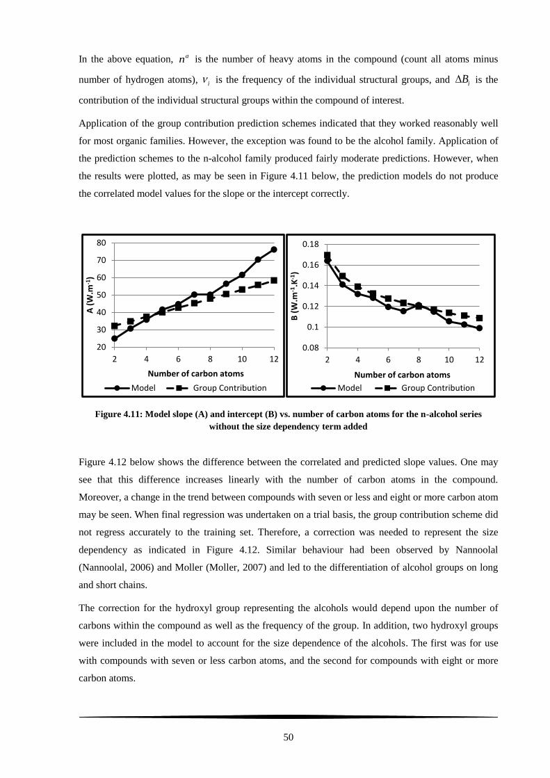
50

In the above equation, an is the number of heavy atoms in the compound (count all atoms minus

number of hydrogen atoms), i is the frequency of the individual structural groups, and iB is the

contribution of the individual structural groups within the compound of interest.

Application of the group contribution prediction schemes indicated that they worked reasonably well

for most organic families. However, the exception was found to be the alcohol family. Application of

the prediction schemes to the n-alcohol family produced fairly moderate predictions. However, when

the results were plotted, as may be seen in Figure 4.11 below, the prediction models do not produce

the correlated model values for the slope or the intercept correctly.


without the size dependency term added

Figure 4.12 below shows the difference between the correlated and predicted slope values. One may

see that this difference increases linearly with the number of carbon atoms in the compound.

Moreover, a change in the trend between compounds with seven or less and eight or more carbon atom

may be seen. When final regression was undertaken on a trial basis, the group contribution scheme did

not regress accurately to the training set. Therefore, a correction was needed to represent the size

dependency as indicated in Figure 4.12. Similar behaviour had been observed by Nannoolal

(Nannoolal, 2006) and Moller (Moller, 2007) and led to the differentiation of alcohol groups on long

and short chains.

The correction for the hydroxyl group representing the alcohols would depend upon the number of

carbons within the compound as well as the frequency of the group. In addition, two hydroxyl groups

were included in the model to account for the size dependence of the alcohols. The first was for use

with compounds with seven or less carbon atoms, and the second for compounds with eight or more

carbon atoms.

20

30

40

50

60

70

80

2 4 6 8 10 12

A (

W.m

-1)


Model Group Contribution

0.08

0.1

0.12

0.14

0.16

0.18

2 4 6 8 10 12

B (

W.m

-1.K

-1)



51

Figure 4.12: Error between model and group contribution predicted slope vs. number of carbon atoms for

the n-alcohol series

Previous work within the group found the size dependency to exist for associating compounds, such as

the alcohols, amines and ketones, and the larger hydrocarbon families of alkanes and alkenes (Moller,

2007). However, within this work, it was found that the size dependence was negligible for most

associating compounds with the only exception being the alcohols.

The modification of the group contribution schemes included the addition of two extra terms. The

initial term takes into account the new size dependent structural contributions. The second term

accounts for the size dependent constants. This was done in preference to a correction being included

for the alcohols, as further modification of the model may be done at a later date if and when more

data becomes available.

The final group contribution prediction schemes are as follows:

1 1 1

n mc

i i j j k

i j k

A A n A A

(4.8)

1 1 1

ln ( )exp

a n mc

i i j j kai j k

nB B n B B

n

(4.9)

In equations (4.8) and (4.9) above, the subscript

i represents all size independent groups

j represents the size dependent groups (viz. –OH) and

k represents the size dependent group constants

The term cn is included to account for the number of carbon atoms in the size dependency.

-10

-5

0

5

10

15

20

0 2 4 6 8 10 12 14

Erro

r b

etw

ee

n m

od

el a

nd

gro

up

co

ntr

ibu

tio

n s

lop

e (

W.m

-1)


52

The application of the size dependency within the alcohol family accounts for the interaction between

the hydroxyl group and its surroundings. Within smaller compounds the –OH group would have a

larger effect on the surrounding atoms. However, as the size (number of atoms) of the compound

increases, the –OH group would have a smaller and more negligible effect on the entire compound.

As may be seen in Figure 4.13 below, the size dependency terms improve the correlation between the

model parameters and those predicted via the respective group contribution schemes.

Figure 4.13: Model slope (A) and intercept (B) vs. number of carbon atoms for the n-alcohol series with

the size dependency term added

20

30

40

50

60

70

80

2 4 6 8 10 12

A (

W.m

-1)



0.08

0.1

0.12

0.14

0.16

0.18

2 4 6 8 10 12

B (

W.m

-1.K

-1)

Number of carbon atoms Model Group Contribution

53

5. Results and Discussion

The development of a simple correlating equation for a set of experimental data may be considered as

a “curve fitting” exercise (Moller, 2007). However, after the data correlation is complete, creation of a

prediction model is required for group contribution models. The regression of a group contribution

type model to experimental data is not as simple as the correlation of experimental data to a single

correlating equation. The regression process in this work required numerous steps in the validation of

the experimental data and the different trends followed by the various organic families. Moreover, the

validation of data was dependent upon the correlation of the data with the group contribution model

equations. This was to ensure that the best and most correct fit to the data was obtained.

It is due to the above aspects in the development of a group contribution model, viz. data correlation of

a single equation to various trends amongst various chemical families, that inaccuracies and

unforeseen problems may appear when the model is complete. Similarly, there are numerous reasons

for different results being obtained from the various models and equations for the prediction,

interpolation and extrapolation of liquid thermal conductivity. A simple equation may not regress well

to all the experimental data within a training set. However, it is the aim of a group contribution method

to be able to provide accurate predictions for all the families contained within the training set.

Figure 5.1: Liquid thermal conductivity vs. temperature for heptane (Gmehling et al., 2009)

Another aspect that was considered was the temperature range of the experimental data being used.

The properties of a compound close to the melting point and normal boiling point may differ from the

54

trends followed by the compound as a liquid, as may be seen in Figure 5.1 above. Below the normal

boiling point the liquid property of a compound is determined at a reference pressure of one

atmosphere. Above the normal boiling point, the compound must be considered along the saturation

curve which exists at higher pressures so that liquid values may be obtained for the property.

As was mentioned previously under Data validation, data at the saturation curve were used where

available in the development of the new model. The change in the slope, as seen in Figure 5.1 above,

was assumed to contribute an insignificant percentage towards the overall relative mean deviation.

However, there is a limited amount of reliable experimental data available above the boiling point

(Chemistry, 2012). With the experimental data from the DDB, the range of temperature for which

reliable predictions may be made was increased to between reduced temperatures of approximately 0.3

to 0.8. However, within the training set many compounds had much smaller temperature ranges, often

between reduced temperatures of approximately 0.4 and 0.7.

5.1. Hydrocarbon Compounds

Hydrocarbon compounds are the simplest of all the organic compounds, consisting of only two

elements, namely carbon and hydrogen. They are the easiest family to represent using the group

contribution approach and are thus used as the framework in the creation of most prediction methods.

The simplest of the hydrocarbons are the n-alkanes, where each consecutive compound in the series

has one extra CH2 group than the previous compound. Consequently, if a property follows the group

contribution scheme, the n-alkane family should follow a perfect trend that may be represented in a

linear or linearized form as seen in Figure 5.2 below.

Figure 5.2: Model slope (A) and intercept (B) vs. number of carbon atoms for the n-alkanes

Moreover, if a method is able to predict the property of the n-alkanes and subsequently the n-alkene

family accurately then the method displays potential of being applicable to the other hydrocarbon

families and potentially all organic liquids.

55

A review of the model constants for the n-alkane series revealed that the larger compounds did not

follow the expected trends very well. This may be attributed to much more data being available for

compounds containing ten or less carbon atoms within the n-alkane series. This would result in the

regression forcing the group contribution schemes to fit better to the compounds for which more data

is available. In this case, this would be the smaller hydrocarbon compounds. Moreover, from the

complete training set of 331 compounds, 267 have ten or fewer carbon atoms.

Therefore, higher errors arose mainly amongst the larger compounds in the series. Regression of the

group contribution schemes found that the model constants A and B for the n-alkanes correlated

accurately to the scheme equations (Eqns. (4.5) and (4.7)) and the results are shown in Table 5.1. The

accuracy of the regression may be seen in Figure 5.3 below for tetradecane.

Figure 5.3: Liquid thermal conductivity vs. temperature for tetradecane (data from the DDB (Gmehling et

al., 2009))

Subsequently, although there was limited data available for cyclic alkanes and numerous structural

isomers, the model fitted the available experimental data fairly accurately.

0.07

0.08

0.09

0.10

0.11

0.12

0.13

0.14

0.15

0.16

290 330 370 410 450

Th

erm

al C

on

du

cti

vit

y

(W.m

-1.K

-1)

Temperature

Proposed Method Experimental Data Sastri & Rao (1993)Nagvekar & Daubert (1987) Lakshmi & Prasad (1992) Sato & Reidel (1977)

56


hydrocarbons for the different models used.

ND = Nagvekar and Daubert (1987), SRa = Sastri and Rao (1993), SRe = Sato and Reidel (1977), LP = Lakshmi and Prasad (1992)

Group

Number of compounds Relative mean deviation (%)

Proposed

Method ND SRa SRe LP

Proposed


Hydrocarbons 88 75 83 88 88 2.77 6.33 5.45 9.38 11.38

Alkanes 47 44 47 47 47 2.50 5.63 5.97 14.15 19.47

Non-cyclic alkanes 36 36 36 36 36 2.16 5.24 5.49 14.07 19.90

Cyclic alkanes 6 6 6 6 6 5.23 10.29 10.20 15.93 14.94

Alkenes 16 14 16 16 16 5.07 22.36 9.73 9.16 10.79

Non-cyclic alkenes 12 10 12 12 12 5.55 24.20 10.95 10.26 12.43

Cyclic alkenes 5 4 5 5 5 4.22 16.08 5.16 5.37 6.55

Aromatic hydrocarbons 25 17 20 25 25 2.58 4.16 4.16 5.20 4.30

Application of the method to the alkene family was limited as there were fairly few alkene compounds

(16 compounds) as compared to alkane (47 compounds). However, compared to the prediction

capability of previous methods, the current group contribution scheme allows much better correlation

and prediction for the thermal conductivity of the alkene family.

No alkyne experimental data was found within literature. It was also evident from all other group

contribution models for thermal conductivity that there was no experimental thermal conductivity data

for alkyne components available for public or academic use. A search through other thermophysical

property databases such as Beilstein (Beilstein, 2008), and ChemSpider (ChemSpider) also indicated

no available alkyne data.

Application of the method to aromatic compounds consisted of the use of structural groups

representing a double bonded carbon atom within an aromatic ring. This was consistent with the work

from previous methods (Olivier, 2010, Moller, 2007). A review of experimental data for the aromatic

hydrocarbons indicated that majority of the data consisted of structural isomers and data following

arene substitution patterns. There was insufficient data available to allow development of a correction

to account for isomers. However, there was a noted improvement in the prediction for aromatic

compounds as compared to previous methods.

57

Table 5.2: Relative mean deviation [%] of liquid thermal conductivity prediction for hydrocarbon

compounds. The number in superscript is the number of data points used; the main number is the RMD

for the respective reduced temperature range.

Tr Proposed

Method

Nagvekar &

Daubert (1987)

Sastri & Rao

(1993)

Sato & Reidel

(1977) Lakshmi &

Prasad (1992)

0.3 – 0.4 2.35108

7.0698

6.74105

5.88108

6.27108

0.4 - 0.5 2.30695

5.32654

4.96674

8.09695

10.35695

0.5 - 0.6 2.541381

6.411340

4.791360

9.391378

10.551378

0.6 - 0.7 3.36521

7.07490

7.27506

12.34516

15.77516

0.7 - 0.9 5.22114

6.28104

7.98105

7.61107

14.60107

0.3 - 0.9 2.732819

6.282686

5.492750

9.412804

11.452804

As may be seen in Table 5.2, the majority of the data for the hydrocarbon compounds fell between the

reduced temperatures of 0.4 to 0.7. The highest errors were found between the reduced temperatures of

0.7 to 0.9 as this was the range wherein data from along the saturated liquid curve was used. As

mentioned earlier, the trend of the data along the saturation curve deviates slightly from that of the

other data. It was seen that although the method of Sastri and Rao (Sastri and Rao, 1993) was

developed to account for this deviation, the proposed method still achieved superior results.

5.1.1. Forcing Rules

It was found in previous work (Moller, 2007) that the contributions for the structural groups of -CH3,

>CH2, >CH- and >C< for bonds within a hydrocarbon compound followed a linear trend when plotted

against the molecular weight of the groups (as shown in Figure 5.4 below). This would be expected as

there is a difference in one hydrogen atom between successive groups from the CH3 down to the C

atom.

58

Figure 5.4: Group contributions (∆A) for -CH3, >CH2, >CH- and >C< vs. their respective molecular

weight

Regression was undertaken using the respective group contribution schemes for the structural

contributions. It was found that regression yielded trends for the hydrocarbon structural groups that

deviated somewhat from the linear scheme. Forcing functions where therefore implemented to ensure

a more linear fit and thus “physically realistic results”.

5.2. Oxygen compounds

Development of physical property prediction methods have always been more difficult for oxygenated

compounds. This is especially true in the case of hydrogen bonding compounds. Since hydrogen

bonding is stronger than other intermolecular forces in non-electrolytic liquids, more energy is

required to dissociate intermolecular contacts.

As illustrated in Table 5.3, thermal conductivity at the normal boiling point drastically increases with

an increase of the number of oxygen atoms within a compound. This increase also depends upon the

type of bond the oxygen atoms are involved in (3-hexanone and 1-hexanol).

Table 5.3: Liquid thermal conductivity of hexane and 4 different oxygenated hexane compounds at their

normal boiling points (Gmehling et al., 2009)

Compound Thermal Conductivity

(W.mol-1

.K-1

)

Number of

Oxygen Bonds

n-Hexane 0.0996 0

3-Hexanone 0.1233 1 (Ketone)

1-Hexanol 0.1177 1 (Alcohol)

1,6-Hexanediol 0.1775 2 (Alcohol)

1,2,6-Hexanetriol 0.2314 3 (Alcohol)

59

These different types of inter-molecular bonding may be represented using different structural groups.

However, temperature dependence of intra-molecular bonding is not representable using the model

developed here and thus contributes to the errors between predicted values and experimental values.

Results for the oxygenated compounds and a comparison with the selected literature methods are

presented in Table 5.4 below. As was expected, the deviations obtained for oxygenated compounds

were higher than in case of the hydrocarbon compounds.


oxygenated compounds for the different models used.


Group


Proposed


Proposed


All Oxygenated Compounds 142 76 138 141 141 4.76 8.79 16.43 15.53 24.21

Carboxylic Acids 3 2 3 3 3 0.60 4.01 8.89 10.72 10.18

Alcohols 27 24 27 27 27 5.04 5.96 4.93 14.52 21.23

Aromatic Alcohols 2 2 2 2 2 8.75 1.77 4.46 8.41 20.22

Aliphatic Alcohols 25 22 25 25 25 4.81 6.25 4.96 14.91 21.29

Diols 6 4 6 6 6 6.31 7.87 8.74 31.15 46.70

Ethers 16 12 16 16 16 7.26 11.05 13.90 10.57 14.43

Esters 74 25 73 74 74 4.33 10.60 18.01 16.58 26.13

Ketones 7 7 7 7 7 5.80 9.20 22.12 5.91 14.84

Aldehydes 3 1 2 2 2 2.80 1.34 6.25 2.23 2.06

Non-Cyclic Carbonates 1 0 0 1 1 0.05 - - 0.68 20.74

There was a vast improvement obtained for the prediction of ethers, esters and ketones as can be seen

from a comparison of the relative mean deviations with older methods in Table 5.4. The prediction for

carboxylic acids can be seen to be greatly improved as well; however, as only three compounds were

available for regression to the group contribution model this does not provide a very good

representation of the carboxylic acid family. A similar conclusion may be drawn for aldehydes and

aromatic alcohols. Application of the method to aliphatic alcohols was fairly similar in accuracy as

compared to the Sastri and Rao [1993] method (Sastri and Rao, 1993) (4.81 % compared to 4.96 %

respectively).

Only one compound was available for regression of the group contribution value for non-cyclic

carbonates. It was not possible to remove use of this structural group and allocate the compound to

other structural groups as the carbonate structural group (-OCOO-) is one of the main groups as

defined within previous work. Moreover, use of this group increases the applicability of the new

60

model, as the previous methods were unable to account for carbonates. The result was therefore

accepted, however the result should be used with caution, even though a similar low value of the

thermal conductivity was predicted using the Sato and Reidel method (Poling et al., 2004).

Figure 5.5: Liquid thermal conductivity vs. reduced temperature for 1,2-Ethanediol [Data obtained from

DDB (Gmehling et al., 2009)]

In case of diols, ethanediol and propanediol were left out of the regression. This was done as the

thermal conductivity for these two compounds exhibited an untypical temperature dependence (similar

to that of water), as shown in Figure 5.5. Similarly, thermal conductivity of glycols could not be

predicted as they follow a similar curvature as shown in Figure 4.3 under Model Development.

As seen in Table 5.5, the proposed method produced slightly higher deviations for the reduced

temperature range of 0.7 to 0.9 for hydrocarbons. Although there were few data points available for

the low temperature range of 0.4 to 0.5, the method produced greatly reduced prediction errors as

compared to previous methods.

It should be noted that the group contribution methods are more often applied to the prediction of

properties for larger and more complex compounds, for which no experimental data are available.

These components are often not stable at higher reduced temperatures.

61

Table 5.5: Relative mean deviation (RMD) [%] of liquid thermal conductivity prediction for oxygenated



Tr Proposed

Method

Nagvekar &

Daubert (1987)

Sastri & Rao

(1993)

Sato & Reidel

(1977)

Lakshmi &

Prasad (1992)

0.3 - 0.4 2.6697

4.417 31.65

90 20.17

97 31.65

97

0.4 - 0.5 4.41479

6.79166

18.26472

16.38479

26.69479

0.5 - 0.6 4.91762

8.67403

14.22745

13.73760

21.2760

0.6 - 0.7 5.09486

9.32253

15.19477

14.86484

23.59484

0.7 - 0.9 5.81146

13.0164

17.46140

21.72140

29.8140

0.3 - 0.9 4.791970

8.78893

16.511924

15.551960

24.261960

5.3. Halogen compounds

Experimental data for fluorinated and chlorinated compounds were available largely for compounds

containing less than five carbon atoms (50 % of the fluorine compounds and 79 % of the chlorine

compounds). The number of structural groups used for these families were therefore kept to a

minimum to allow more data per group and hence increase the reliability of the results. A large

amount of this data consisted of multifunctional compounds. Instead of utilising group interaction

terms to account for the effect of the different halogen groups on each other, structural groupings were

used. These groupings differentiated between aromatic and non-aromatic carbon bonds, and between

carbons with one or two other halogen atoms bonded to it and in this way accounted for the

interactions between the different halogen groups (Moller et al., 2008).

The bromine data consisted primarily of mono-functional compounds with very few multi-functional

compounds. Therefore, only two structural groups (bromine attached to aromatic carbon and bromine

attached to non-aromatic carbon) as used by Moller et al. (Moller et al., 2008) were regressed for. Use

of groups to account for multi-functional bonds was seen as unnecessary due to the lack of

multifunctional compounds containing bromine.

62


halogenated compounds and the different models used.


Group


Proposed


Proposed


Halogenated Compounds 66 32 66 66 66 6.02 7.77 21.91 10.59 37.27

Fluorinated 20 10 20 20 20 7.00 12.63 24.29 11.24 42.08

Chlorinated 14 9 14 14 14 4.92 10.07 6.04 5.55 8.31

Brominated 11 6 11 11 11 1.97 2.91 10.09 6.04 10.14

Iodinated 2 2 2 2 2 3.39 5.32 1.41 7.04 17.86

Results for the different families of halogenated compounds are provided in Table 5.6. Only one

functional group was used for iodinated compounds as there were only two compounds containing

iodine within the training set. The data for the iodine compounds were obtained from four different

sources dating as far back as 1965 and 1951 (Gmehling et al., 2009). As stated previously, data from

as far back as this may not be accurate as the experimental equipment used was not of as high a

standard as that available today. However, due to the lack of data, the compounds were kept for use.

Results for the proposed method were better across the temperature range as opposed to other

methods, as seen in Table 5.7 below, with a better overall RMD.

Table 5.7: Relative mean deviation (RMD) [%] of liquid thermal conductivity prediction for halogenated



Tr Proposed

Method

Nagvekar &

Daubert (1987)

Sastri & Rao

(1993)

Sato & Reidel

(1977)

Lakshmi &

Prasad (1992)

0.3 - 0.4 8.9170

2.768 15.4

70 10.7

70 28.39

70

0.4 - 0.5 5.1235

4.2660

21.63235

9.69235

23.88235

0.5 - 0.6 4.71347

6.72134

20.93347

9.97347

27.23347

0.6 - 0.7 5.28283

9.03105

24.93283

11.84283

39.48283

0.7 - 0.9 8.62249

12.2898

24.8249

10.85249

64.54249

0.3 - 0.9 5.991184

8.22405

22.511184

10.591184

37.411184

The regression results for halogenated compounds were superior to previous methods, with large

improvements (greater than 30%) being obtained for fluorine, chlorine and bromine compounds. The

main problem encountered was higher deviations for data at the low and high end of the temperature

range. The higher deviation for the halogenated compounds as compared to the other families was

attributed to the large amount of scatter within the data. Moreover, the available data, being mainly

63

from multifunctional compounds, resulted in higher errors being obtained for the model slopes as

compared to the model intercept. A better account for the errors was shown when the halogen

structural groups were plotted against their atomic radii and the trends checked.

5.3.1. Group 17 Trends

The halogen group atoms of fluorine, chlorine, bromine and iodine followed a similar trend to that of

the hydrocarbon groups as shown in Figure 5.4. This trend is structurally related to the groups and

therefore may be represented using the molecular weight, as was done for the hydrocarbon structural

groups. However, as the halogen structural groups contain only one atom each it was noted that it

would be more appropriate using the atomic radii of the compounds to represent the trend. The

structural contributions were found to be inversely proportional to the atomic radii squared and are

shown for the slope and intercept of the model equation in Figure 5.6 and Figure 5.8.

Figure 5.6 below shows that the group contribution values for the halogen atoms follow a linear trend

when plotted against the respective structural group atomic radii squared. The atomic radius was used

as a representation of the size of the respective atoms. However, it was found that fluorine did not

follow the trend perfectly. This was explained by looking at the electronegativities of the halogens in

Table 5.8.

Figure 5.6: Model intercept (B) contribution vs. respective atomic radii squared for a halogen attached to

a non-aromatic carbon (♦ - fitted group value)

The Pauling electronegativities of chlorine, bromine and iodine increased linearly; however, the value

for fluorine was slightly higher than the expected value if the trend followed by the lower three atoms

of the family was extrapolated backwards. This phenomenon may be explained by looking at the

electronic configuration of the halogen atoms.

64

Figure 5.7: Pauling electronegativities vs. atomic radii for the halogen atoms

Table 5.8: Electronic configuration for the first four halogen atoms from the periodic group 17

(Chemistry, 2012)

Element No. of electrons/shell

Fluorine 2, 7

Chlorine 2, 8, 7

Bromine 2, 8, 18, 7

Iodine 2, 8, 18, 18, 7

Fluorine was shown to have the least amount of electrons in its orbitals and would thus form the

smallest atom from the four halogens. It therefore has the highest electronegativity from the halogen

groups. Although all the halogen compounds form hydrogen halides; fluorine is the only one that acts

both as a hydrogen bond donor and acceptor. Possible hydrogen bond acceptors must exhibit small

size and high electron density, such as fluorine, nitrogen and oxygen.

The above trends of Figure 5.6 and Figure 5.7 were therefore used for defining a set of forcing rules

which the halogen structural groups within halogenated compounds must follow. Figure 5.8 shows

that chlorine, which has data from 4 compounds behind the regression for its contribution, does not

match the expected trend. Although fluorine with 6 compounds, bromine with 10 compounds and

iodine with 2 compounds form a much better fit. Therefore, extrapolating from the straight line trend

followed by the other halogen atoms, a new, more physically realistic value was calculated for

chlorine. The results obtained from using this new value produced slightly higher errors, but a more

physically realistic representation for chlorine would provide a much better prediction than a value

regressed from one or two datasets which may or may not have been erronous.

65

Figure 5.8: Model slope (A) contribution vs. respective atomic radii squared for a halogen attached to a

non-aromatic carbon (♦ - fitted group value, ◊ - new group value)

As mentioned previously, due to the small amount of experimental data being available to back up

regression results, if the few data sets available contain “bad data”, this may render a method useless.

Therefore, correlation techniques such as that used here for the halogen groups and previously for the

hydrocarbon groups, may be applied to other families when there is little data available for regression

of certain structural groups, for example, primary, secondary and tertiary amines or alcohols.

Figure 5.9: Model intercept (B) contribution vs. respective atomic radii squared for a halogen attached to

an aromatic carbon (♦ - fitted group value)

66

Figure 5.10: Model slope (A) contribution vs. respective atomic radii squared for a halogen attached to an

aromatic carbon (♦ - fitted group value, ◊ - new group value)

The only problem when utilising such a correlation technique when there is little or no data available,

is the ability to test the results obtained. For example, regression for group 37 from Figure 5.10 above

was done with only one available data set for the training set. With no test data, the accuracy of the

result cannot be tested. After applying the linear fit as shown in Figure 5.10, the training set error for

the data used for structural group regression increased, but so did the confidence in the contribution

for group 37 as it has a physical relevance added to it. Deviations shown in Table 5.6 and Table 5.7

were calculated using the more physically realistic contributions.

5.4. Nitrogen compounds

Data for nitrogen containing compounds did not show any untypical trends and no modifications of

the group contribution model were required. Ammonia has much weaker hydrogen bonding than water

and the behaviour found for diols should be much less pronounced in the case of diamines (for which

no data were available). There were data for fewer compounds available for regression of the

structural contributions as compared to the other families. However, the method produced a much

lower deviation as compared to previous methods as shown in Table 5.9. The method produces

notably lower errors for all the reduced temperature ranges, as shown in Table 5.10, except the highest

one of 0.7 to 0.9.

The method has greater applicability for nitrogen compounds (31 compounds) compared to other

group contribution methods (23 compounds for Nagvekar and Daubert (Nagvekar and Daubert, 1987)

being the highest). The only problem encountered was data available for only one compound for the

regression of the 6-membered aromatic nitrogen ring structural group (group 88). Although the data

utilized was obtained from a reliable reference, usage of the group should be done with caution as

there is no way to validate the accuracy of the structural contribution. The structural group was

67

therefore included in the method so that it is available if required, and so that it may be recalculated at

a later stage when more data becomes available.


nitrogen compounds and the different models used.


Group


Proposed


Proposed

Method ND Sra SRe LP

All nitrogen compounds 31 23 21 31 31 3.25 14.43 16.42 8.67 13.68

Amides 3 1 0 3 3 3.47 2.11 - 19.22 32.12

Nitrates 4 4 4 4 4 2.41 11.50 18.41 6.11 7.92

Amines 18 13 17 18 18 3.27 5.69 14.20 9.36 13.46

Primary amines 9 5 8 9 9 2.89 6.86 18.29 14.17 20.88

Secondary amines 5 5 5 5 5 2.70 7.78 17.44 5.64 7.48

Tertiary amines 4 3 4 4 4 3.98 2.38 6.71 5.96 8.38

6-membered aromatic

nitrogen rings 1 0 0 1 1 0.84 - - 2.12 20.96

Nitriles 5 4 0 5 5 6.60 4.32 - 1.82 10.94

Nitrites 4 4 4 4 4 2.41 11.50 18.41 6.11 7.92

Table 5.10: Relative mean deviation (RMD) [%] of liquid thermal conductivity prediction for nitrogen



Tr Proposed

Method

Nagvekar &

Daubert (1987)

Sastri & Rao

(1993)

Sato & Reidel

(1977)

Lakshmi &

Prasad (1992)

0.3 - 0.4 3.248 1.3

5 16.05

3 8.9

8 20.1

8

0.4 - 0.5 3.0374

8.8757

15.6942

10.6974

19.2374

0.5 - 0.6 3.3488

21.4565

16.0552

8.2888

12.2288

0.6 - 0.7 2.434

11.8429

17.2330

8.3634

7.4734

0.7 - 0.9 4.3219

14.4619

17.8319

3.0919

7.2419

0.3 - 0.9 3.17223

14.43175

16.42146

8.67223

13.68223

68

Figure 5.11: Group contributions (∆A) for –NH2, >NH and >N- vs. their respective molecular weight

Results for the tertiary amines indicated that the method of Nagvekar and Daubert (Nagvekar and

Daubert, 1987) provided a better prediction with a lower error. However, the higher deviations in case

of the new method are accepted and recommendation is made for its use as the primary and

secondary amines provided greatly improved results as compared to past methods. Moreover, as may

be seen in Figure 5.11, when the three different amine structural groups were graphed against their

respective radii squared, it was seen that the results follow a similar trend as displayed in Figure 5.4

for the hydrocarbon structural groups.

5.5. Other compounds

Table 5.11: Relative mean deviation [%] of thermal conductivity estimation for all other organic families

and the different models used.


Group


Proposed


Proposed


Sulphur Compounds 2 0 2 2 2 10.09 - 10.87 3.52 5.64

Phosphates 1 0 0 1 1 0.78 - - 1.43 33.26

Metal Groups 1 0 0 1 1 0.26 - - 1.64 20.84

As can be seen from the results in Table 5.11, there was extremely little experimental data available

for regression of structural contributions for any other families. However, as the data is available, the

structural groups are included in the method as they may not be covered by other group contribution

methods. The results for these families should be used with extreme caution as there are minimal data

backing them up.

69

The families of phosphates and the metal groups (stannane being the only one) produce similar results

to that of the Sato and Reidel method (Poling et al., 2004), and this may thus provide a little

confidence for the usage of these groups. The two sulphur compounds used were structural isomers,

and thus produced a high error as the method cannot account for structural isomerism.

5.6. Testing the method

An indication of the versatility of the method cannot be derived from the results obtained utilizing the

training set as this would just be an indication of the fit of the data by the model. To test how well the

method actually works outside of the training set, a set of data external to the training set is required.

The problem encountered when creating such a test set for thermal conductivity is the lack of

experimental data external to that which was used to create the training set. Therefore, test data were

obtained via two different methods.

The first way was by extrapolation of data at one atmosphere from compounds which had

experimental data at pressures higher than one atmosphere only. This provided a test set of 65

compounds. However, a closer analysis of the data produced useable data for only a third of the

compounds. To expand upon the test set, all the data which were excluded from the training set was

reviewed. Compounds with three or more data points, which did not deviate too drastically when

compared to results obtained from literature methods, were kept to be incorporated into a test set. The

advantage of using these data is that it provides a larger test set with a wider range of data; the

disadvantage is that these data were left out of the training set due to large scatter in the data or trends

which did not match the respective family trends.

Table 5.12: Relative mean deviation [%] of thermal conductivity estimation for the test set data and the

different models used.


Group


Proposed


Proposed


Hydrocarbons 10 9 10 10 10 7.23 11.94 7.10 13.84 24.08

Halogen Compounds 4 2 4 4 4 12.97 16.44 4.33 15.62 60.33

Oxygen Compounds 20 12 19 20 20 6.68 26.40 12.76 11.70 17.22

Nitrogen Compounds 4 3 1 4 4 7.24 7.23 15.35 6.56 8.73

Overall 38 26 34 38 38

7.68 9.32 10.44 13.90 23.63

As shown in Table 5.12, utilisation of the test set indicates that the new method provides an

improvement on previous methods, having a lower relative mean deviation of 7.68 % for a test set of

70

38 compounds which consisted of 328 data points. There is an indicated large improvement for

prediction of oxygen-containing compounds with a relative mean deviation of 6.68 % compared to the

lowest comparable value of 11.70 % for the method of Sato and Reidel (Poling et al., 2004). The

halogen compounds exhibit the largest error for the test set. This could be attributed to the fact that the

data were extrapolated from the pressure only data set. However, the halogens yield a much smaller

error for the method of Sastri and Rao (Sastri and Rao, 1993).

Table 5.13: Relative mean deviation [%] of thermal conductivity estimation for the test set data for

halogenated compounds and the different models used.


Compound

Relative mean deviation (%)

Proposed

Method SRa ND SRe LP

1,1-Dichloro-2,2,3,3,3-pentafluoropropane R225ca 10.08 2.81 20.09 17.62 49.70

1,3-Dichloro-1,1,2,2,3-pentafluoropropane R225cb 14.53 2.26 - 16.59 50.50

1,1,1,2,3,3,3-Heptafluoropropane [R227ea] 15.40 3.51 - 15.34 107.99

1,1,2-Trichloroethane 11.90 9.13 12.79 13.06 9.28

This result could be interpreted in two other ways. Looking at the prediction results in Table 5.13, one

may assume that data for similar compounds was utilised by Sastri and Rao (Sastri and Rao, 1993) in

their training set. Or that their training set contained a small amount of halogen compounds which

followed the same trends as the test set compounds. According to the results of the training set, the

current method produces a much better fit for halogenated compounds than that of Sastri and Rao

(Sastri and Rao, 1993). Therefore, a larger test set would be required to provide a fuller picture of the

shortcomings of the current method as compared to previous methods.

Similarly, a larger test set is required for the nitrogen compounds as the training set indicates a vast

improvement as compared to previous methods.

5.7. Final results

The new method was regressed to a training set of 331 compounds consisting of 6282 data points. This

was almost half of the initial 11000 data points available for modelling. Many of the data points were

of low quality and had to be removed from the training set as mentioned earlier. As shown in Table

5.14 below, the training set produced an overall relative mean deviation of 3.87 % for the 331

compounds as compared to the lowest literature method of Nagvekar and Daubert (Nagvekar and

Daubert, 1987) which produced a relative mean deviation of 7.03 % for 206 compounds.

71

Table 5.14: Relative mean deviation [%] of thermal conductivity estimation for the new method and

literature methods.

D = Nagvekar and Daubert (1987), SRa = Sastri and Rao (1993), SRe = Sato and Reidel (1977), LP = Lakshmi and Prasad (1992)

Group


Proposed


Proposed


Hydrocarbons 88 75 83 88 88

2.77 6.33 5.45 9.38 11.38

Oxygenated Compounds 142 76 138 141 141

4.76 8.79 16.43 15.53 24.21

Nitrogen Compounds 31 23 21 31 31

3.25 14.43 16.42 8.67 13.68

Halogenated Compounds 66 32 66 66 66

6.02 7.77 21.91 10.59 37.27

Sulphur Compounds 2 0 2 2 2

10.09 - 10.87 3.52 5.64

Phosphates 1 0 0 1 1

0.78 - - 1.43 33.26

Metal Groups 1 0 0 1 1

0.26 - - 1.64 20.84

All Compounds 331 206 310 330 330

3.87 7.03 11.25 11.91 18.96

The new method provides improved estimation of thermal conductivity behaviour for non-electrolyte

organic liquids. It has a wider range of applicability than previous methods in that it covers a wider

range of different components. The method uses 68 different first order structural groups which were

regressed against the training set. However, some structural contributions were obtained from only one

or two compounds. These structural groups should be used with caution as they were kept for use in

the method to provide a greater applicability and a guide against which future models may be

compared.

Table 5.15: Regression and prediction results for respective group contribution methods as reported in

literature and calculated for the training set for the new model

Method Groups Corrections

Reported in

respective papers

Calculated from

training set

NC NP RMD (%) NC NP RMD (%)

Sastri & Rao (1999) 32 7 208 748 5.6 Not implemented

Rodenbush et al. (1999) 84 10 228 1487 2.5 Not implemented

Sastri & Rao (1993) 29 6 No results provided 310 11.25

Nagvekar & Daubert (1987) 84 8 226 2089 5.9 206 7.03

Current Method 67 1 331 6282 3.87

Compared to previous methods, only the methods of Sastri and Rao (1993 and 1999) (Sastri and Rao,

1993, Sastri and Rao, 1999) utilized a small amount of structural groups for their method. This

simplified approach can provide a good and simple prediction method for thermal conductivity

72

predictions; however, when being applied to compounds with complicated and/or highly polar

structures, the method may not be able to account for the different effects especially in case of atoms

with higher electronegativities and may fail to provide an accurate prediction.


compared to literature methods for training set data


compared to literature methods for test set data

0

10

20

30

40

50

60

70

80

90

100

10 20 30 40 50 60 70 80 90 100

Co

mp

on

en

ts in

eac

h r

ange

(%

)

Error Range (%)

Lakshmi & Prasad Sato & Reidel Nagvekar & Daubert

Sastri & Rao Current Method

0

10

20

30

40

50

60

70

80

10 20 30 40 50 60 70

Co

mp

on

en

ts in

eac

h r

ange

(%

)

Error Range (%)

Proposed Method Nagvekar & Daubert Sastri & Rao

Sato & Reidel Lakshmi & Prasad

73

The new method which has been developed provides a large improvement over previous group

contribution methods. As may be seen in Figure 5.12, the predicted deviations for over 90 % of the

training set fall below an error of 10 %. And similarly in Figure 5.13, the predictive deviations for

almost 70 % of the test set fall below an error of 10 %. The compounds for which higher errors were

found are those which either consist of three or less carbons, or are structural isomers. The results for

the test set were found to be lower than the training set, due to the type of data used as mentioned

above. However the overall relative mean deviation for the test set was lower than the literature

method.

74

6. Conclusions

Based on previous group contribution methods developed within our group, a more accurate and

precise method with a better temperature dependency is presented for liquid thermal conductivity

prediction. The model has a wider range of applicability than previous correlations and models, which

were based on smaller experimental data sets.

The group contribution scheme accounts for size dependence for alcohols. This was not extended to

other types of organic compounds such as ketones, carboxylic acids, etc., as there was insufficient data

to model the respective behaviours. Linear forcing functions were incorporated into regression for the

structural contributions to ensure the contributions correlated with structural behaviour.

The input requirements of the new method are the molecular structure, the normal boiling point, the

number of heavy atoms (non-hydrogen) and the number of carbon atoms in the compound of interest.

The method produces a low overall relative mean deviation, with a much improved method for almost

all of the families. Application of the method to a training set of 331 compounds (6264 data points)

produced a relative mean deviation (RMD) of 3.87 %.

Applicability to data outside the training and performance of the model was tested using an external

set of liquid thermal conductivity data. The RMD produced was 7.68 % for 38 compounds (328 data

points). This error was found to be high as the test set contained data extrapolated from experimental

data at elevated pressures, and other less reliable data which was excluded from the training set. From

the results it may be concluded that the method may be applied to components outside the training set

with reasonable confidence.

75

7. Recommendations

Evaluation of this project in conjunction to the continuation of the overall work of the group indicates

the following requirements for future work to be undertaken:

Development of a pressure dependence term for the proposed method may be undertaken;

Experimental work should be undertaken to increase the amount of thermal conductivity data

available for the chemical families which have data for less than five compounds;

Use of the new experimental data should be made to improve upon the existing model and

recalculate the values for structural contributions were too few compounds were used to

calculate the group parameters in this work.

76

8. References

Drx-i-ytx fluid liquid material themal conductivity testing equipment products, buy drx-i-ytx. 2010

[cited Available from: http://www.alibaba.com/product-

gs/249577259/DRX_I_YTX_Fluid_Liquid_Material_Thermal_Conductivity_Testing_Equipm

ent.html]

Assael, M. J., Charitidou, E. & Wakeham, W. A. (1989), Thermal conductivity of liquids: Prediction

based on a group-contribution scheme. International Journal of Thermophysics, 10, 779-791.

Assael, M. J., Trusler, J. P. M. & Tsolakis, T. F. (1998), Thermophysical properties of fluids - an

introduction to their prediction, London, Imperial College Press.

Beilstein, F. K. (2008), Crossfire beilstein. Frankfurt.

Chemistry, R. S. o. (2012), Rsc visual elements periodic table.

ChemSpider. Chemzoo. [cited 2009; Available from: http://www.chemspider.com]

Cordes, W. & Rarey, J. (2002), A new method for the estimation of the normal boiling point of non-

electrolyte organic compounds. Fluid Phase Equilibria, 201, 409-433.

Ely, J. F. & Hanley, H. J. M. (1981), Prediction of transport properties. 1 viscosity of fluids and

mixtures. Industrial and Engineering Chemistry Fundamentals, 20, 323-332.

Ely, J. F. & Hanley, H. J. M. (1983), Prediction of transport properties. 2. Thermal conductivity of

pure fluids and mixtures. Industrial and Engineering Chemistry Fundamentals, 22, 90-97.

Fujioka, K., Sekiguchi, T. & Kato, Y. (2006), Experimental and simulation analysis of reactor design

for chemical heat pump aiming to enhance thermal transportation Ecostock Meeting.

Gmehling, J., Rarey, J. & Menke, J. (2009), Dortmund data bank. Oldenburg.

Hoover, W. G. (1991), Computational statistical mechanics.

Horrocks, J. K. & McLaughlin, E. (1963), Temperature dependence of the thermal conductivity of

liquids. Transactions of the Faraday Society, 59, 1709.

Horvath, A. L. (1992), Molecular design - chemical structure generation from the properties of pure

organic compounds, New York, Elsevier.

Jamieson, D. T. (1979), Thermal conductivity of liquids. Journal of Chemical and Engineering Data,

24, 244-246.

Klaas, D. M. & Viswanath, D. S. (1998), A correlation for the prediction of thermal conductivity of

liquids. Industrial & Engineering Chemistry Research, 37, 2064.

Lakshmi, D. S. & Prasad, D. H. L. (1992), A rapid method for thermal conductivity of pure fluids.

Chemical Engineering Journal, 48, 211-214.

Mathias, P. M., Parekh, V. S. & Miller, E. J. (2002), Prediction and correlation of the thermal

conductivity of pure fluids and mixtures, including the critical region. Industrial &

Engineering Chemistry Research, 41, 989-999.

Millat, J., Dymod, J. H. & Nieto de Castro, C. A. (2005), Transport properties of fluids – their

correlation, prediction and estimation, New York, Cambridge University Press.

http://www.alibaba.com/product-gs/249577259/DRX_I_YTX_Fluid_Liquid_Material_Thermal_Conductivity_Testing_Equipment.html



http://www.chemspider.com/

77

Moller, B. (2007), "Development of an improved group contribution method for the prediction of

vapour pressures of organic compounds", Masters Thesis, University of KwaZulu Natal.

Moller, B., Rarey, J. & Ramjugernath, D. (2008), Estimation of the vapour pressure of non-electrolyte

organic compounds via group contributions and group interactions. Journal of Molecular

Liquids, 143, 52-63.

Nagvekar, M. & Daubert, T. E. (1987), A group contribution method for liquid thermal conductivity.

Industrial & Engineering Chemistry Research, 26, 1362.

Nannoolal, Y. (2006), "Development and critical evaluation of group contribution methods for the

estimation of critical properties, liquid vapour pressure and liquid viscosity of organic

compounds", PHD Thesis, Kwa-Zulu Natal.

Nannoolal, Y., Rarey, J. & Ramjugernath, D. (2007), Estimation of pure component properties part 2:

Estimation of critical data by group contribution. Fluid Phase Equilibria, 252, 1-27.

Nannoolal, Y., Rarey, J. & Ramjugernath, D. (2008), Estimation of pure component properties part 3:

Estimation of the vapor pressure of non-electrolyte organic compounds via group

contributions and group interactions. Fluid Phase Equilibria, 269, 117-133.

Nannoolal, Y., Rarey, J. & Ramjugernath, D. (2009), Estimation of pure component properties. Part 4:

Estimation of the saturated liquid viscosity of non-electrolyte organic compounds via group

contributions and group interactions. Fluid Phase Equilibria, 281, 97-119.

Nannoolal, Y., Rarey, J., Ramjugernath, D. & Cordes, W. (2004), Estimation of pure component

properties, part 1: Estimation of the normal boiling point of non-electrolyte organic

compounds via group contributions and group interactions. Fluid Phase Equilibria, 226, 45-

63.

Nemzer, V. G., Nemzer, L. V. & Pugach, V. V. (1996), Thermal conductivity of poly(ethylsiloxane)

liquids at high pressures. Journal of Chemical and Engineering Data, 41, 848-851.

Nieto de Castro, C. A. (1990), Thermal conductivity and diffusivity of fluids. IN Cremers, C. J. &

Fine, H. A. (Eds.) Thermal Conductivity 21. New York, Plenum Press.

Olivier, E. (2010), "A new group contribution method for the estimation of surface tension for non-

electrolyte organic compounds", Masters Thesis, University of KwaZulu Natal.

Palmer, G. (1948), Thermal conductivity of liquids. Industrial & Engineering Chemistry Research, 40,

89-92.

Poling, B. E., Prauznitz, J. M. & O'Connell, J. P. (2004), The properties of gases and liquids, New

York, McGraw-Hill.

Rarey, J. (2009), Gvt09e 02 pure component properties. Fundamentals of Selection, Synthesis and

Design of Thermal Separation Processes. DDB.

Reid, R. C., Prauznitz, J. M. & Sherwood, T. K. (1977), The properties of gases and liquids, New

York, McGraw-Hill.

78

Reidel, L. (1951), Neue warmeleitfahigkeitsmessungen an organischen flussigkeiten. Chemie

Ingenieur Technik, 23, 321-324.

Rodenbush, C. M., Viswanath, D. S. & Hsieh, F. (1999), A group contribution method for the

prediction of thermal conductivity of liquids and its application to the prandtl number for

vegetable oils. Industrial & Engineering Chemistry Research, 38, 4513-4519.

Sakiadis, B. C. & Coates, J. (1955), Studies of thermal conductivity of liquids part i. AIChE Journal,

1, 275-288.

Sakiadis, B. C. & Coates, J. (1957), Studies of thermal conductivity of liquids part iii. AIChE Journal,

1, 121-126.

Sastri, S. R. S., Mohanty, S. & Rao, K. K. (1997), Prediction of saturated liquid volumes of organic

compounds. Fluid Phase Equilibria, 132, 33-46.

Sastri, S. R. S. & Rao, K. K. (1993), Quick estimating for thermal conductivity. Chemical

Engineering, 100, 106-107.

Sastri, S. R. S. & Rao, K. K. (1999), A new temperature-thermal conductivity relationship for

predicting saturated liquid thermal conductivity. Chemical Engineering, 74, 161-169.

Smith, J. M., Van Ness, H. C. & Abbot, M. M. (2005), Introduction to chemical engineering

thermodynamics, McGraw-Hill.

ThermTest-Inc. Thermtest - transient plane source - how it works. 2010 [cited Available from:

http://www.thermtest.com/content/228455]

Wagner, W. (1977), A new correlation method for thermodynamic data applied to the vapor pressure

curve on argon, nitrogen and water. London: IUPAC Thermodynamic Tables Project Centre.

Wikipedia. Wikipedia. 2010 [cited 2009; Available from: http://en.wikipedia.org/wiki]

http://www.thermtest.com/content/228455

http://en.wikipedia.org/wiki

I

Appendix A: Group Contribution Tables

Ink

No. Name

Description

Examples

Priority

∆A

∆B

Aliphatic Carbon Groups

33 † =C-C= Conjugated double bonds (chain) trans-1,3-Pentadiene 71 -8.434 0.2742

32 † =C-C= Conjugated double bonds (ring) 1,3-Cyclopentadiene 91 17.880 -2.5138

29 -CH3 Methyl group attached to a ring carbon Methylcyclohexane 92 15.01 -2.813

26 CH2= Double bonded carbon at the end of a

chain/ring 1-Nonene 113 13.33 -2.164

27 -C= Double bonded carbon in a chain with 2

carbon neighbours 2-Methyl-2-pentene 114 -10.10 1.201

24 -CH2- CH2 in a ring attached to an

electronegative atom 1,4-Dioxane 118 7.65 -1.860

15 >C< C in a ring attached to an electronegative

atom Perfluorocyclopentane 119 -34.63 1.170

21 >C= Double bond between carbons in a ring 1,3-Cyclopentadiene 124 10.37 -1.217

12 >C< C in a ring 1,1-Dimethylcyclopentane 128 -39.11 2.764

14 >CH- CH in a ring attached to an electronegative

atom Cyclopentanol 131 -14.43 -0.288

4 -CH2- CH2 in a chain n-Butane 136 2.33 -0.636

5 >CH- CH in a chain 3-Ethylpentane 137 -16.18 1.095

6 >C< C in a chain 2,2,4-Trimethylpentane 138 -34.82 2.756

10 -CH2- CH2 in a ring Cyclohexane 139 4.67 -1.218

11 >CH- CH in a ring Methylcyclohexane 140 -9.75 0.547

1 -CH3 Methyl group attached to a non-

electronegative atom 2,2-Dimethylbutane 141 16.16 -2.589

20 =C- Double bonded carbon in a chain with only

1 carbon neighbour 2-Heptene 142 4.83 -1.096

7 -CH2- CH2 in a chain attached to an

electronegative atom Ethylenediamine 143 -3.94 -0.919

2 -CH3 Methyl group attached to an

electronegative atom N-Methylaniline 144 14.42 -2.754

8 -CH< CH in a chain attached to an

electronegative atom 5-Ethyl-2-nonanol 145 -20.36 0.818

9 >C< C in a chain attached to an electronegative

atom tert-Butanol 147 -37.15 1.966

II

Ink

No. Name

Description

Examples

Priority

∆A

∆B

Aromatic Carbon Groups

16

-CH(a)< CH in an aromatic ring Benzene 116 6.17 -1.220

17

>C(a)< C in an aromatic ring Propylbenzene 121 -11.00 0.726

18

>C(a)< C in an aromatic ring attached to an

electronegative atom Aniline 123 -12.04 0.322

19

=C(a)< Aromatic carbon attached to three aromatic

neighbours Naphthalene 125 -6.19 -0.086

3

-CH3 Methyl group attached to an aromatic atom 1-Methyl naphthalene 146 17.40 -2.637

Halogen Groups

38 F-C-1Halo Fluorine attached to a carbon with one other

halogen atom Perfluorocyclopentane 61 19.057 -2.1214

43 Cl-C-1Halo Chlorine attached to a carbon with one other

halogen atom

2-Bromo-2-chloro-

1,1,1-trifluoroethane 65 21.743 -2.4678

149 Cl-C=(1 Halo) Chlorine attached to a double bonded carbon

with one other halogen atom Tetrachloroethylene 66 14.202 -2.6812

44 Cl-C-2Halo Chlorine attached to a carbon with two other

halogen atoms

1,1,1-Trichloroethane

[R140a] 67 16.272 -2.4102

40 Cl- Chlorine attached to a non-aromatic carbon Chloroethane 70 16.852 -2.2692

41 Cl-C(a) Chlorine attached to an aromatic carbon Chlorobenzene 76 20.216 -2.5325

42 Cl-C= Chlorine attached to a double bonded carbon 2-Chloro-1,3-butadiene 77 23.059 -1.9803

35 F- Fluorine attached to a non-aromatic carbon 1-Fluoropentane 78 28.679 -1.4986

37 F-C(a) Fluorine attached to an aromatic carbon Fluorobenzene 79 31.255 -2.2799

39 F-C-2Halo Fluorine attached to a carbon with two other

halogen atoms

1,1,1,2-Tetrachloro-

2,2-difluoroethane

[R112a]

93 14.832 -2.3602

47 † I- Iodine attached to carbon Ethyl iodide 94 1.147 -3.3472

46 Br-C(a) Bromine attached to an aromatic carbon Bromobenzene 132 12.348 -2.9920

145 Br-C-2Halo Bromine attached to a carbon with two other

halogen atoms

Tribromomethane

[R20B3] 133 13.232 -2.7571

45 Br- Bromine attached to a non-aromatic carbon 1,2-Dibromoethane 135 6.135 -2.7263

III

Ink

No. Name

Description

Examples

Priority

∆A

∆B

Oxygen groups

61 † O=C(-O-)2 Carbonate diester Carbonic acid dimethyl ester 8 25.492 -1.1897

49* -OH (n=<7) OH Group attached to a small

molecule (n =< 7) 2-Methyl-hexanol 21 2.150 -0.1041

50 † C(a)-OH Aromatic OH 2-Naphthol 22 -4.051 -1.5286

72 -CONH< Amide with two substituents

attached to the nitrogen

N,N-Dimethylformamide

(DMF) 25 11.442 0.8726

58 >C=O Ketone Acetone 60 0.546 -0.2229

153* -OH (n>7) OH Group attached to a large

molecule (n > 7) 5-Ethyl-2-nonanol 62 3.074 -0.1443

175** -OH (n=<7) Short OH group constant (n=<7) 2-Methyl-hexanol 64 7.450 -1.0202

48 C(a)-COOH Aromatic COOH Benzoic acid 74 13.727 -3.1523

66 -OCOO- Carbonates O-C=O & -O Propylene carbonate 81 18.249 -2.0575

70 -CONH< Amide with no substituents Acetamide 96 26.620 -3.0101

52 -O- Aromatic oxygen Furan 97 12.776 -1.4955

51 -O- Ether oxygen Diethyl ether 98 7.507 0.3052

55 -COO - Formic acid ester Formic acid ethyl ester 99 23.158 -2.8564

59 -CHO Aldehyde in Chain Acetaldehyde 101 12.744 -2.4582

53 -COOH Carboxylic acid Group Pentanoic acid 102 4.982 -1.6203

54 -COO - Ester in a chain 1,3-Benzenedicarboxylic

acid dimethyl ester 104 6.527 -1.0405

IV

Ink

No. Name

Description

Examples

Priority

∆A

∆B

Nitrogen Groups

89 -CtN CN group attached to a carbon Acetonitrile 11 25.543 -2.6877

93 -NH- Secondary amines (ring) attached to

carbon Morpholine 12 9.092 0.5287

82 -NH- Secondary amines (chain) attached to a

carbon Dibutylamine 15 9.835 0.3294

75 NO2- Nitro group attached to a non-aromatic

carbon Nitromethane 26 28.361 -3.1016

76 NO2- Nitro group attached to an aromatic carbon Nitrobenzene 28 29.557 -3.4053

88 † =N- Aromatic nitrogen in a six-membered ring 2-Methylpyridine 29 22.279 -0.8005

84 -N< Tertiary amine attached to carbon N,N-dimethylaniline 36 -12.576 1.1656

81 NH2- Primary amine attached to an aromatic

carbon Aniline 57 75.000 -2.2536

80 NH2- Primary amine attached to a non-aromatic

carbon Ethylenediamine 59 5.175 -0.9976

Other Groups

95 † P(O)O3- Phosphate trimester Methyl diphenyl phosphate 8 3.692 -0.5891

110 † >Sn< Stannane with four carbon neighbours Tetramethylstannane 24 -26.549 3.2233

100 † -S- Thioether Ethyl methyl sulfide 81 11.579 0.0759

* indicates size dependency

** indicates a constant

† Group contribution value must be used with caution as there is minimal experimental data

behind this value

V

Appendix B: Sample Calculations

Compound: 2-Ethylhexanol-2-ene

Number of carbon atoms: 8

Number of heavy atoms: 9

Normal Boiling Point: 464.4 K

Temperature: 323.15 K

Group Atoms Frequency ∆A ∆B OH Correction ∆A Total ∆B Total

1 1,9 2 16.161 -2.589 N 32.323 -5.177

4 2,3,8 3 2.330 -0.636 N 6.990 -1.907

7 6 1 -3.938 -0.919 N -3.938 -0.919

20 4 1 4.832 -1.096 N 4.832 -1.096

27 5 1 -10.103 1.201 N -10.103 1.201

153 7 8 * 3.074 -0.144 Y 24.593 -1.155

54.697 -9.054

1 1

ln(9)exp 9.054

9

0.1097 . .

B

B W m K

1 1

(1 )

54.697 323.15(1 ) (0.1097)464.4464.4

0.145 . .

BB

A T BTT

W m K

Calculated thermal conductivity: 0.145 W.m-1

.K-1

Experimental thermal conductivity: 0.143 W.m-1

.K-1

Error = 0.145 0.143

100 1.74%0.143

* NB: Frequency of the alcohol group is multiplied by the number of carbon atoms in the compound

VI

Compound: 1,2-Dibromo-1-chloro-1,2,2-trifluoroethane (Freon 113B2)



Normal Boiling Point: 366.02K

Temperature: 323.15K


9 2,5 2 -37.15 1.97 N -74.30 3.93

39 3,7,8 3 14.83 -2.36 N 44.50 -7.08

44 4 1 16.27 -2.41 N 16.27 -2.41

145 1,6 2 13.23 -2.76 N 26.46 -5.51

12.93 -11.07

1 1

ln(8)exp 11.07

8

0.0562 . .

B

B W m K

1 1

(1 )

12.93 323.15(1 ) (0.0562)366366

0.0604 . .

BB

A T BTT

W m K


.K-1


.K-1

Error = 0.0676 0.0604

100 10.71%0.0604

VII

Compound: Ethylbenzene






1 1 1 16.16 -2.59 N 16.16 -2.59

4 2 1 2.33 -0.636 N 2.33 -0.64

16 4,5,6,7,8 5 6.17 -1.22 N 30.85 -6.10

17 3 1 -11.00 0.73 N -11.00 0.73

38.34 -8.60

1 1

ln(8)exp 8.06

8

0.107 . .

B

B W m K

1 1

(1 )

38.34 353.15(1 ) (0.107)409.3409.3

0.1198 . .

BB

A T BTT

W m K


.K-1


.K-1

Error = 0.1175 0.1198

100 1.98%0.1198

VIII

Compound: 1,3-Cyclopentadiene






10 1 1 4.67 -1.218 N 4.67 -1.22

21 2,5 2 10.37 -1.217 N 20.74 -2.43

32 3&4 1 17.88 -2.514 N 17.88 -2.51

43.29 -6.17

1 1

ln(5)exp 6.17

5

0.1374 . .

B

B W m K

1 1

(1 )

43.29 283.15(1 ) (0.1374)313.8313.8

0.1509 . .

BB

A T BTT

W m K


.K-1


.K-1

Error = 0.1465 0.1509

100 3.00%0.1509

IX

Compound: Naphthalene






16 2,3,4,5,7,8,9,10 8 6.17 -1.220 N 49.36 -9.76

19 1,6 2 -6.19 -0.086 N -12.38 -0.17

36.98 -9.93

1 1

ln(10)exp 9.93

10

0.1016 . .

B

B W m K

1 1

(1 )

36.98 438.83(1 ) (0.1016)491.3491.3

0.1096 . .

BB

A T BTT

W m K


.K-1


.K-1

Error = 0.1121 0.1096

100 2.21%0.1096

X

Compound: Biphenyl



Normal Boiling Point: 529K



16 3 to 12 10 6.17 -1.220 N 61.70 -12.20

17 1,2 2 -11.00 0.726 N -22.00 1.45

39.70 -10.75

1 1

ln(12)exp 10.75

12

0.1080 . .

B

B W m K

1 1

(1 )

39.70 472.65(1 ) (0.1080)529529

0.1166 . .

BB

A T BTT

W m K


.K-1


.K-1

Error = 0.1193 0.1166

100 2.26%0.1166

XI

Compound: 2-propanol






1 3,4 2 16.16 -2.589 N 32.32 -5.18

8 2 1 -20.36 0.818 N -20.36 0.82

49 1 3 * 2.15 -0.10 Y 6.45 -0.31

Correction

175 1 7.45 -1.02 Y 7.45 -1.02

25.86 -5.69

1 1

ln(4)exp 5.69

4

0.1391 . .

B

B W m K

1 1

(1 )

25.86 303.15(1 ) (0.1391)355.5355.5

0.1468 . .

BB

A T BTT

W m K


.K-1


.K-1

Error = 0.1396 0.1468

100 5.16%0.1468

* NB: Frequency of the alcohol group is multiplied by the number of carbon atoms in the compound

XII

Appendix C: Example Calculation Using the Mathias et al. Model

All equations used are obtained from the paper of Mathias et al. (Mathias et al., 2002) unless stated

otherwise.

General Definitions

System Conditions (T, P)

Physical Property Parameters

Example Component: n-Hexane

Reference Component: Methane

Critical density calculated from critical volume:

Calculation of viscosity and ideal gas heat capacity:

Parameters fitted to data obtained from the DDB (Gmehling et al., 2009).

Viscosity calculated from DIPPR 102 (Gmehling et al., 2009) equation for vapour viscosity.

kmol 1000mol

mPa 0.001Pa

kPa 1000Pa

dm 0.1m

R 8.314J

mol K

mW 0.001W

Pa 106Pa

T 298.15K

P 101.3kPa

M 86.177kg

kmol

Tc 507.40K

Vc 370.0cm

3

mol

0.29750

Pc 3014.419kPa

Mo 16.043kg

kmol

Tco 190.60K

Vco 99.0cm

3

mol

o 0.011

Pco 4600.155kPa

co

Mo

Vco

co 0.1621kg dm3

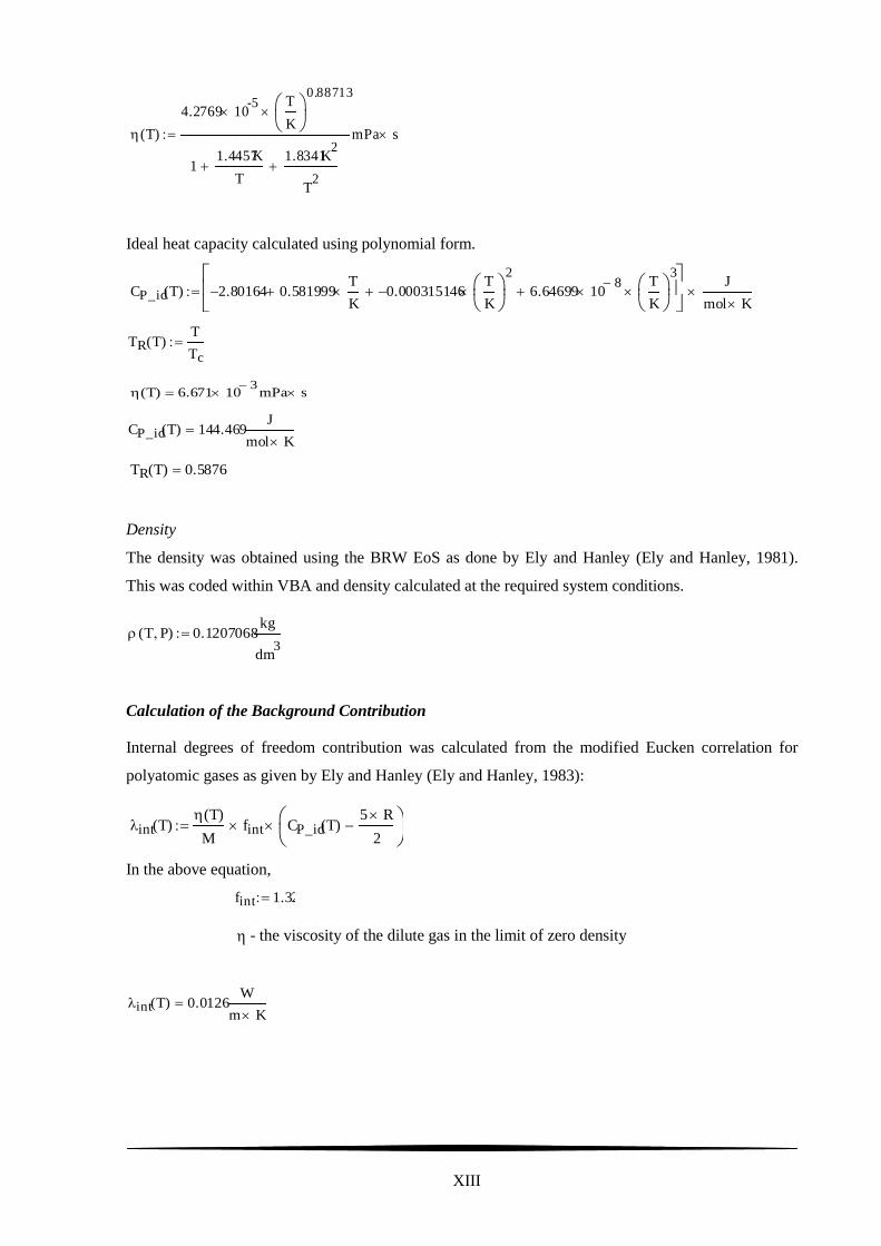
XIII

Ideal heat capacity calculated using polynomial form.

Density

The density was obtained using the BRW EoS as done by Ely and Hanley (Ely and Hanley, 1981).

This was coded within VBA and density calculated at the required system conditions.

Calculation of the Background Contribution

Internal degrees of freedom contribution was calculated from the modified Eucken correlation for

polyatomic gases as given by Ely and Hanley (Ely and Hanley, 1983):

In the above equation,

f

- the viscosity of the dilute gas in the limit of zero density

T( )

4.2769 10-5

T

K

0.88713

11.4457K

T

1.8341K2

T2

mPa s

CP_id T( ) 2.80164 0.581999T

K 0.000315146

T

K

2

6.64699 108

T

K

3

J

mol K

TR T( )T

Tc

T( ) 6.671 103

mPa s

CP_id T( ) 144.469J

mol K

TR T( ) 0.5876

T P( ) 0.1207068kg

dm3

int T( ) T( )

Mfint CP_idT( )

5 R

2

fint 1.32

int T( ) 0.0126W

m K

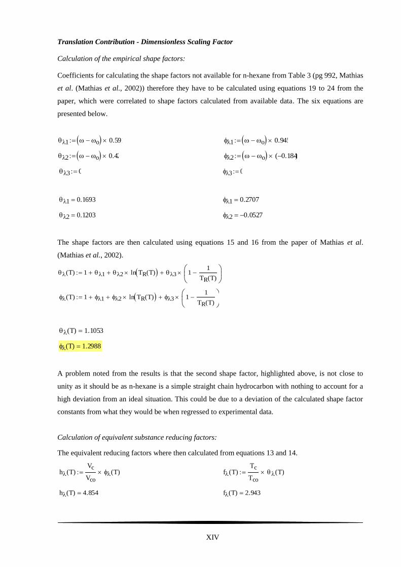
XIV

Translation Contribution - Dimensionless Scaling Factor

Calculation of the empirical shape factors:

Coefficients for calculating the shape factors not available for n-hexane from Table 3 (pg 992, Mathias

et al. (Mathias et al., 2002)) therefore they have to be calculated using equations 19 to 24 from the

paper, which were correlated to shape factors calculated from available data. The six equations are

presented below.

The shape factors are then calculated using equations 15 and 16 from the paper of Mathias et al.

(Mathias et al., 2002).

A problem noted from the results is that the second shape factor, highlighted above, is not close to

unity as it should be as n-hexane is a simple straight chain hydrocarbon with nothing to account for a

high deviation from an ideal situation. This could be due to a deviation of the calculated shape factor

constants from what they would be when regressed to experimental data.

Calculation of equivalent substance reducing factors:

The equivalent reducing factors where then calculated from equations 13 and 14.

1 o 0.591

2 o 0.42

3 0

1 o 0.945

2 o 0.184( )

3 0

1 0.1693

2 0.1203

1 0.2707

2 0.0527

T( ) 1 1 2 ln TR T( ) 3 11

TR T( )

T( ) 1 1 2 ln TR T( ) 3 11

TR T( )

T( ) 1.1053

T( ) 1.2988

h T( )Vc

Vco

T( )

h T( ) 4.854

f T( )Tc

Tco

T( )

f T( ) 2.943

XV

Calculation of dimensionless scaling factor:

This was calculated from equation 7. The scaling factor thus gives the deviation of the reference fluid

from the compound of interest.

Translation Contribution - Reference Contribution

The reference contribution was calculated using the method of Ely and Hanley (Ely and Hanley,

1983). All equations for the calculation of the reference contribution were taken from the paper of Ely

and Hanley (Ely and Hanley, 1983) unless stated otherwise.

The equivalent reducing factors are used to calculate the reference density and temperature for use in

calculating the reference contribution.

Coefficients for the three parts of the reference contribution:

Coefficient B is obtained from the FORTRAN example (Assael et al., 1998) as the B values from the

Ely and Hanley paper gave results which were wrong.

F T( )Mo

M

1

2

f T( )

1

2 h T( )

2

3

F T( ) 0.2582

o T P( ) T P( ) h T( )

o T P( ) 0.58591kg

dm3

To T( )T

f T( )

To T( ) 101.324K

A

7.197708227

85.67822264

12.471834689

984.62522975

0.35946850007

69.798412538

872.88332851

B

2.5276292 104

3.3432859 104

1.12

168.00

C

2907741.307

3312874.033

1608101.838

433190.4871

70624.8133

7116.62075

432.51744

14.4591121

0.2037119479

XVI

Calculating the high density contribution:

It was noted that when calculating the high density contribution using the equations provided by Ely

and Hanley, the result obtained was too low. After comparison with the example obtained from a

textbook by Assael et al. (Assael et al., 1998) it was noted that the equation provided a result that was

of by a factor of a thousand. To correct for this, the factor of 10-3

was introduced into the equation.

8.1.1. Calculating the first density correction:

8.1.2. Calculating the dilute gas contribution:

Firstly the dilute gas viscosity had to be calculated. A factor of 10-7

was used as per the example from

Assael et al. (Assael et al., 1998).

exp_part T P( ) A3

A4

To T( )

K

3

2

o T P( )

kg

dm3

0.1

o T P( )

co

1

o T P( )

kg

dm3

0.5

A5

A6

To T( )

K

A7

To T( )

K

2

o T P( ) exp A1

A2

To T( )

K

exp exp_part T P( )( )( ) 1[ ]W

m K 10

3

o T P( ) 0.6546W

m K

T( ) B1

B2

B3

ln

To T( )

K

B4

2

W

m K

T( ) 6.3077 104

W

m K

o T( )

1

9

n

Cn

To T( )

K

n 4( )

3

10.7

Pa s

XVII

Once the viscosity is obtained, the dilute gas contribution is calculated.

Calculating the reference contribution:

Calculating the translational contribution:

Background Term

o T( ) 4.0216 106

Pa s

T( )15 R

4 Moo T( )

T( ) 7.8154 103

W

m K

T( ) 7.8154 103

W

m K

T( )o T P( )

kg

dm3

3.6958 104

W

m K

o T P( ) 0.6546W

m K

o T P( ) T( ) T( )o T P( )

kg

dm3

o T P( )

o T P( ) 0.6628W

m K

trans T P( ) o T P( ) F T( )

F T( ) 0.2582

o T P( ) 0.6628W

m K

trans T P( ) 0.171W

m K

bg T P( ) trans T P( ) int T( )

bg T P( ) 0.1837W

m K

XVIII

Thermal Conductivity Prediction Results from Artist (DDB 2009 (Gmehling et al., 2009)) at

298.15K

Method Result Unit

Nagvekar/Daubert 0.1231 W. m-1

.K-1

Sastri/Rao 0.1168 W. m-1

.K-1

Lakshmi 0.1366 W. m-1

.K-1

Mathias et al. 0.1837 W. m-1

.K-1

Experimental Thermal Conductivity (DDBST (Gmehling et al., 2009)): 0.1168 W. m-1

.K-1

As may be seen from the sample calculation above, application of the predictive method of Mathias et

al. requires an extremely long calculation but thus not provide highly accurate results. The method

was applied to the training set of 331 compounds used for this work and yielded a relative mean

deviation (RMD) of 297 % for 202 compounds.

Table C-1: Relative mean deviation (RMD) of thermal conductivity prediction results for Mathias et al.

(Mathias et al., 2002) (NC = number of compounds)

Group Name NC RMD (%)

Hydrocarbons 80 275.84

Oxygenated Compounds 73 477.57

Halogenated Compounds 47 62.00

All Sulphur Compounds 2 76.73

202 297.01

When the deviations’ for all the compounds to which the method was applied was sorted into different

temperature groups, a noticeable trend was found. The RMD decreased as the reduced temperature

increased. This suggested that the method works better at higher temperatures closer to or at the

critical temperature. However, such a temperature range was not considered in this work.

Table C-2: Relative mean deviation (RMD) of thermal conductivity prediction results for Mathias et al.

(Mathias et al., 2002) (ND = number of data points)

Reduced Temperature ND RMD (%)

0.3 - 0.4 175 453.74

0.4 - 0.5 1078 633.53

0.5 - 0.6 2121 199.56

0.6 - 0.7 997 80.66

0.7 - 0.9 382 19.56

XIX

Appendix D: Data Validation and Regression Interfaces

Figure D-1: Initial data validation interface

XX

Figure D-2: Data validation interface including a correlation functions to validate trends

XXI

Figure D-3: Structural parameter contribution regression interface

XXII

Figure D-4: Data validation interface utilizing correlation of high pressure data

Documents

A New Group Contribution Method For The … New Group Contribution Method for the Estimation of Thermal Conductivity of Non-Electrolyte Organic Compounds By Onellan Govender [B.Sc