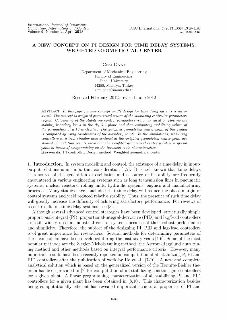
International Journal of InnovativeComputing, Information and Control ICIC International c©2013 ISSN 1349-4198Volume 9, Number 4, April 2013 pp. 1539–1556

A NEW CONCEPT ON PI DESIGN FOR TIME DELAY SYSTEMS:WEIGHTED GEOMETRICAL CENTER

Cem Onat

Department of Mechanical EngineeringFaculty of Engineering

Inonu University44280, Malatya, Turkeycem.onat@inonu.edu.tr

Received February 2012; revised June 2012

Abstract. In this paper, a new concept on PI design for time delay systems is intro-duced. The concept is weighted geometrical center of the stabilizing controller parametersregion. Calculating of the stabilizing control parameters region is based on plotting thestability boundary locus in the (kp, ki) plane and then computing stabilizing values ofthe parameters of a PI controller. The weighted geometrical center point of this regionis computed by using coordinates of the boundary points. In the simulations, stabilizingcontrollers in a trial circular area centered at the weighted geometrical center point arestudied. Simulation results show that the weighted geometrical center point is a specialpoint in terms of compromising on the transient state characteristics.Keywords: PI controller, Design method, Weighted geometrical center

1. Introduction. In system modeling and control, the existence of a time delay in input-output relations is an important consideration [1,2]. It is well known that time delaysas a source of the generation of oscillation and a source of instability are frequentlyencountered in various engineering systems such as long transmission lines in pneumaticsystems, nuclear reactors, rolling mills, hydraulic systems, engines and manufacturingprocesses. Many studies have concluded that time delay will reduce the phase margin ofcontrol systems and yield reduced relative stability. Thus, the presence of such time delaywill greatly increase the difficulty of achieving satisfactory performance. For reviews ofrecent results on time delay systems, see [3].

Although several advanced control strategies have been developed, structurally simpleproportional-integral (PI), proportional-integral-derivative (PID) and lag/lead controllersare still widely used in industrial control systems because of their robust performanceand simplicity. Therefore, the subject of the designing PI, PID and lag/lead controllersis of great importance for researchers. Several methods for determining parameters ofthese controllers have been developed during the past sixty years [4-6]. Some of the mostpopular methods are the Ziegler-Nichols tuning method, the Astrom-Hagglund auto tun-ing method and other methods based on integral performance criteria. However, manyimportant results have been recently reported on computation of all stabilizing P, PI andPID controllers after the publication of work by Ho et al. [7-10]. A new and completeanalytical solution which is based on the generalized version of the Hermite-Biehler the-orem has been provided in [7] for computation of all stabilizing constant gain controllersfor a given plant. A linear programming characterization of all stabilizing PI and PIDcontrollers for a given plant has been obtained in [8,10]. This characterization besidesbeing computationally efficient has revealed important structural properties of PI and

1539

1540 C. ONAT

PID controllers. For example, it was shown that for a fixed proportional gain, the setof stabilizing integral and derivative gains lies in a convex set. This method is very im-portant since it can cope with systems that are open loop stable or unstable, minimumor nonminimum phase. However, the computation time for this approach increases in anexponential manner with the order of the system being considered. It also needs sweep-ing over the proportional gain to find all stabilizing PI and PID controllers which is adisadvantage of the method. An alternative fast approach to this problem based on theuse of the Nyquist plot has been given in [11,12]. An extension of the method given in[11] to the lad-lead controller structure has been given in [13]. A parameter space ap-proach using the singular frequency concept has been given in [14] for design of robustPID controllers. More direct graphical approaches to this problem based on frequencyresponse plots have been given in [15,16]. The major problem for this approach is therequirement for frequency gridding. In [17], a method has been given for computationof stabilizing PI controllers in the parameter plane, (kp, ki)-plane. In this method, theresult of [12] has been used to avoid the problem of frequency gridding. Thus, a veryfast way of calculating the stabilizing values of PI controllers for a given control systemhas been obtained. Recently, a graphical method to compute all feasible gain and phasemargin specifications-oriented PID controllers based on this method has been reported in[18] where, it has considered both parametric uncertainty and varying time delay. As aresult of this study, Kharitonov region is proposed for robust PID controllers for uncertainsystems with time varying delay. None of above mentioned methods have dealt with nu-merically tuning of PI and PID controller parameters. A common trait of these methodsleads to calculating the stability region in the controller parameters space. However, thenumbers of controllers in these regions are endless and it is not clear that which point canbe selected.In this paper, a new concept on PI tuning method based on stabilizing controller param-

eters region for the time delay systems is presented. The concept is weighted geometricalcenter of stabilizing controller parameters region. The region in the controller parameterspace is computed by using the stability boundary locus method [17]. The weighted ge-ometrical center point which can be used as a design preference is computed by meansof the density of stability boundary points. The most important property of the methodis its simplicity and reliability for determining the PI controller parameters according tothe other PI tuning methods in the literature [5,19-21]. In practice, the method providesan algorithmic tool which has guaranteed stability and can be applied to other systems.The paper is organized as follows. The next section summarizes the fundamental prop-

erties of the stability boundary locus technique. In Section 3, the derivation of theweighted geometric center for PI controller tuning is presented. Simulations are con-sidered in Section 4 to illustrate the wisdom of the presented concept. Finally, concludingremarks are given in Section 5.

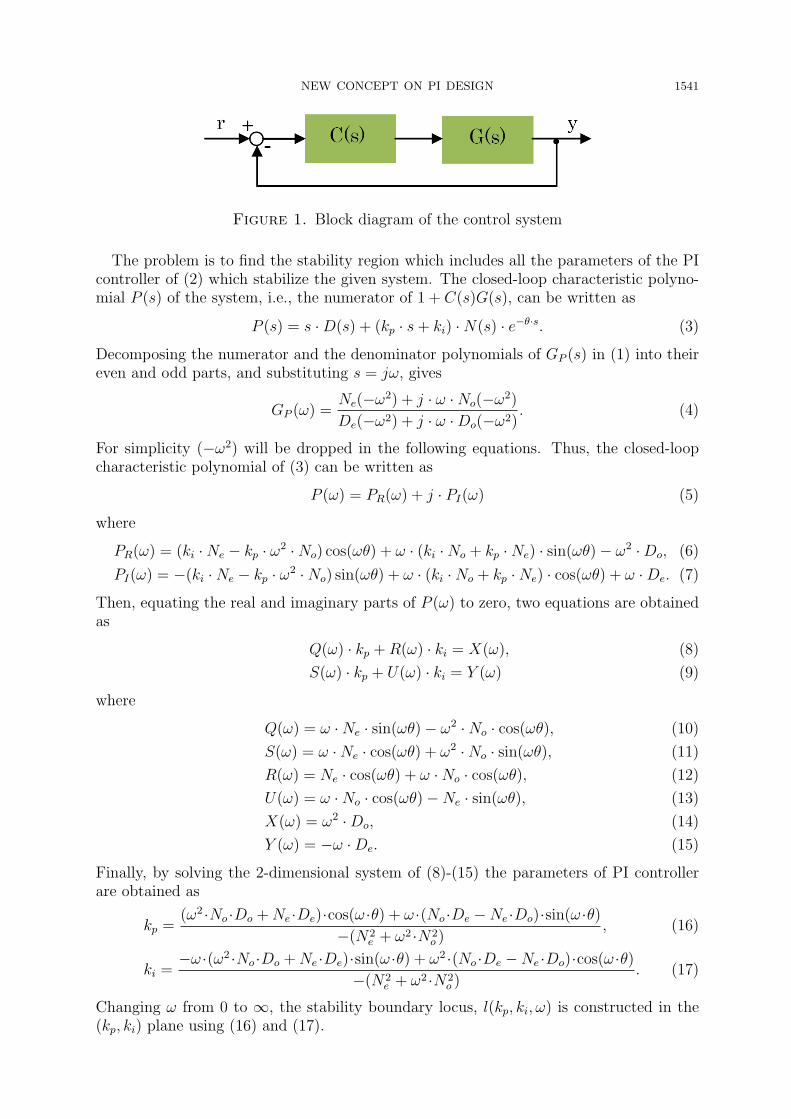
2. Stability Region for a PI Controller. In this section, a method is presented toobtain the stability region using the stability boundary locus approach [17]. Consider thesingle-input (r) single-output (y) (SISO) control system shown in Figure 1 where

G(s) = GP (s) · e−θs =N(s)

D(s)· e−θs (1)

is the plant to be controlled and C(s) is the PI controller of the form

C(s) = kp +kis. (2)

NEW CONCEPT ON PI DESIGN 1541

Figure 1. Block diagram of the control system

The problem is to find the stability region which includes all the parameters of the PIcontroller of (2) which stabilize the given system. The closed-loop characteristic polyno-mial P (s) of the system, i.e., the numerator of 1 + C(s)G(s), can be written as

P (s) = s ·D(s) + (kp · s+ ki) ·N(s) · e−θ·s. (3)

Decomposing the numerator and the denominator polynomials of GP (s) in (1) into theireven and odd parts, and substituting s = jω, gives

GP (ω) =Ne(−ω2) + j · ω ·No(−ω2)

De(−ω2) + j · ω ·Do(−ω2). (4)

For simplicity (−ω2) will be dropped in the following equations. Thus, the closed-loopcharacteristic polynomial of (3) can be written as

P (ω) = PR(ω) + j · PI(ω) (5)

where

PR(ω) = (ki ·Ne − kp · ω2 ·No) cos(ωθ) + ω · (ki ·No + kp ·Ne) · sin(ωθ)− ω2 ·Do, (6)

PI(ω) = −(ki ·Ne − kp · ω2 ·No) sin(ωθ) + ω · (ki ·No + kp ·Ne) · cos(ωθ) + ω ·De. (7)

Then, equating the real and imaginary parts of P (ω) to zero, two equations are obtainedas

Q(ω) · kp +R(ω) · ki = X(ω), (8)

S(ω) · kp + U(ω) · ki = Y (ω) (9)

where

Q(ω) = ω ·Ne · sin(ωθ)− ω2 ·No · cos(ωθ), (10)

S(ω) = ω ·Ne · cos(ωθ) + ω2 ·No · sin(ωθ), (11)

R(ω) = Ne · cos(ωθ) + ω ·No · cos(ωθ), (12)

U(ω) = ω ·No · cos(ωθ)−Ne · sin(ωθ), (13)

X(ω) = ω2 ·Do, (14)

Y (ω) = −ω ·De. (15)

Finally, by solving the 2-dimensional system of (8)-(15) the parameters of PI controllerare obtained as

kp =(ω2 ·No ·Do +Ne ·De)·cos(ω ·θ) + ω ·(No ·De −Ne ·Do)·sin(ω ·θ)

−(N2e + ω2 ·N2

o ), (16)

ki =−ω ·(ω2 ·No ·Do +Ne ·De)·sin(ω ·θ) + ω2 ·(No ·De −Ne ·Do)·cos(ω ·θ)

−(N2e + ω2 ·N2

o ). (17)

Changing ω from 0 to ∞, the stability boundary locus, l(kp, ki, ω) is constructed in the(kp, ki) plane using (16) and (17).

1542 C. ONAT

As a special case, a real root can cross over the imaginary axis at s = 0. Thus, a realroot boundary is obtained by substituting s = 0 in P (s) of (3). Therefore, this specialboundary is determined as

ki = 0. (18)

The stability boundary locus and the real root boundary divide the parameter plane(kp, ki) into stable and unstable regions. The stable region can be obtained by choosinga test point within each region.

Example 2.1. Consider the transfer function of the first order plus time delay (FOPTD)system has the form

G(s) =N(s)

D(s)· e−θs =

1

s+ 1e−0.5·s. (19)

Here, the aim is to obtain all stabilizing values of kp and ki that make the closed loopsystem in Figure 1 stable. The following equations are obtained after equating the realand imaginary part of characteristic to zero.

kp · ω · cos(0.5 · ω)− ki · sin(0.5 · ω) = ω, (20)

kp · ω · sin(0.5 · ω) + ki · cos(0.5 · ω) = −ω2 (21)

The plotting of the stability boundary locus is executed by cooperative analyzing of Equa-tions (20) and (21) for each value of ω. Hereunder, kp, ki pairs are obtained accordinglyto ω values. Then, computed kp, ki pairs are figured in (kp, ki)-plane.Figure 2 shows the stability boundary locus for a range of frequency (0, 10 rad/s) and

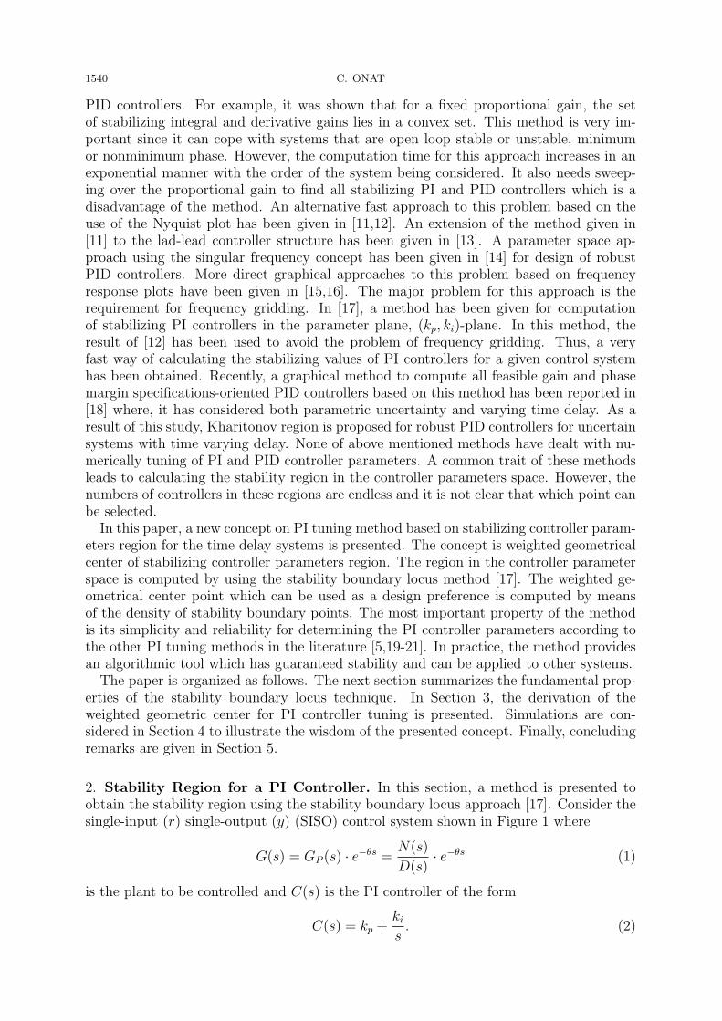
the real root boundary line. It can be observed from this figure that the parameter planeis divided into four regions, namely R1, R2, R3 and R4. By choosing one arbitrary testpoint in each region, the stability region which is the shaded region (R2) shown in Figure

Figure 2. Stability boundaries of the FOPDT system

NEW CONCEPT ON PI DESIGN 1543

Figure 3. Stability region of the system

2 can be determined. Figure 3 shows more clearly R2 for all stabilizing values of kp andki. In this figure, the stability boundary locus is computed for the range of ω [0, ωi]. Theintersection frequency ω is calculated as 3.67 rad/s.

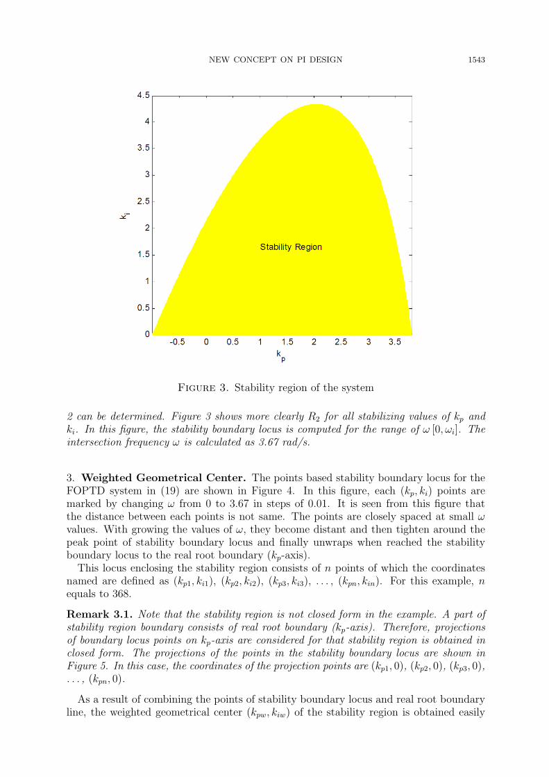
3. Weighted Geometrical Center. The points based stability boundary locus for theFOPTD system in (19) are shown in Figure 4. In this figure, each (kp, ki) points aremarked by changing ω from 0 to 3.67 in steps of 0.01. It is seen from this figure thatthe distance between each points is not same. The points are closely spaced at small ωvalues. With growing the values of ω, they become distant and then tighten around thepeak point of stability boundary locus and finally unwraps when reached the stabilityboundary locus to the real root boundary (kp-axis).

This locus enclosing the stability region consists of n points of which the coordinatesnamed are defined as (kp1, ki1), (kp2, ki2), (kp3, ki3), . . . , (kpn, kin). For this example, nequals to 368.

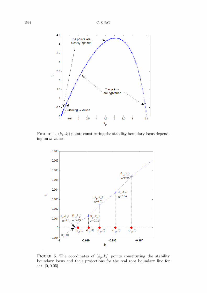
Remark 3.1. Note that the stability region is not closed form in the example. A part ofstability region boundary consists of real root boundary (kp-axis). Therefore, projectionsof boundary locus points on kp-axis are considered for that stability region is obtained inclosed form. The projections of the points in the stability boundary locus are shown inFigure 5. In this case, the coordinates of the projection points are (kp1, 0), (kp2, 0), (kp3, 0),. . . , (kpn, 0).

As a result of combining the points of stability boundary locus and real root boundaryline, the weighted geometrical center (kpw, kiw) of the stability region is obtained easily

1544 C. ONAT

Figure 4. (kp, ki) points constituting the stability boundary locus depend-ing on ω values

Figure 5. The coordinates of (kp, ki) points constituting the stabilityboundary locus and their projections for the real root boundary line forω ∈ [0, 0.05]

NEW CONCEPT ON PI DESIGN 1545

as follows

kpw =1

n

n∑j=1

kpj, (22)

kiw =1

2 · n

n∑j=1

kij. (23)

Thus, the weighted geometrical center using (22) and (23) can be found precisely. It isclear that smaller step size of ω provides greater accuracy.

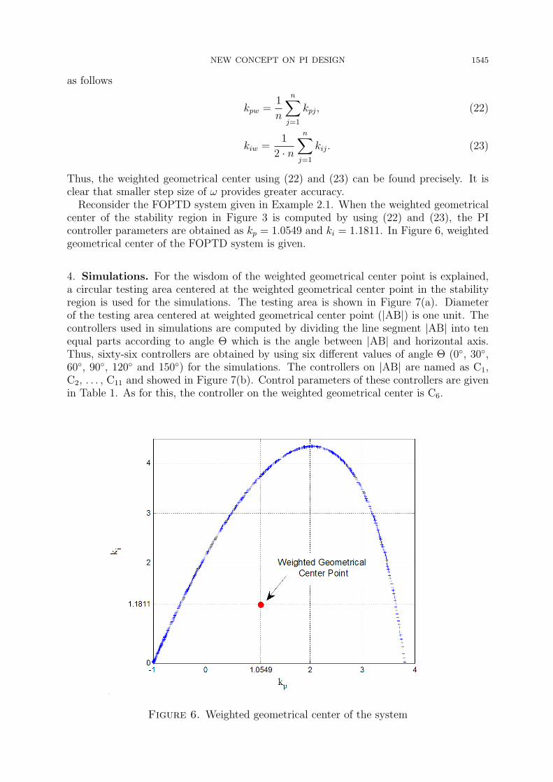
Reconsider the FOPTD system given in Example 2.1. When the weighted geometricalcenter of the stability region in Figure 3 is computed by using (22) and (23), the PIcontroller parameters are obtained as kp = 1.0549 and ki = 1.1811. In Figure 6, weightedgeometrical center of the FOPTD system is given.

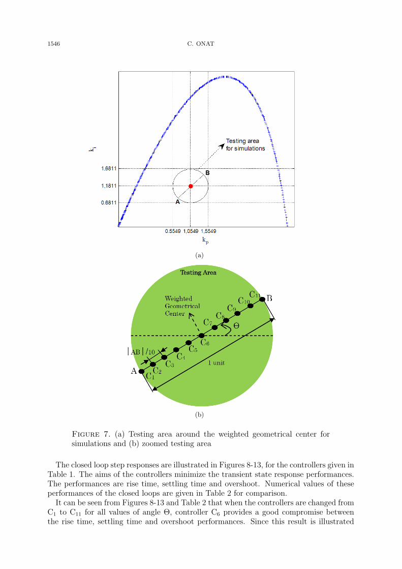
4. Simulations. For the wisdom of the weighted geometrical center point is explained,a circular testing area centered at the weighted geometrical center point in the stabilityregion is used for the simulations. The testing area is shown in Figure 7(a). Diameterof the testing area centered at weighted geometrical center point (|AB|) is one unit. Thecontrollers used in simulations are computed by dividing the line segment |AB| into tenequal parts according to angle Θ which is the angle between |AB| and horizontal axis.Thus, sixty-six controllers are obtained by using six different values of angle Θ (0◦, 30◦,60◦, 90◦, 120◦ and 150◦) for the simulations. The controllers on |AB| are named as C1,C2, . . . , C11 and showed in Figure 7(b). Control parameters of these controllers are givenin Table 1. As for this, the controller on the weighted geometrical center is C6.

Figure 6. Weighted geometrical center of the system

1546 C. ONAT

(a)

(b)

Figure 7. (a) Testing area around the weighted geometrical center forsimulations and (b) zoomed testing area

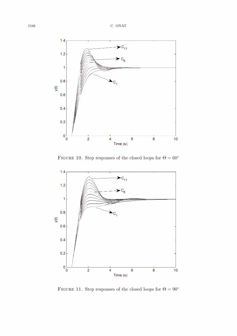
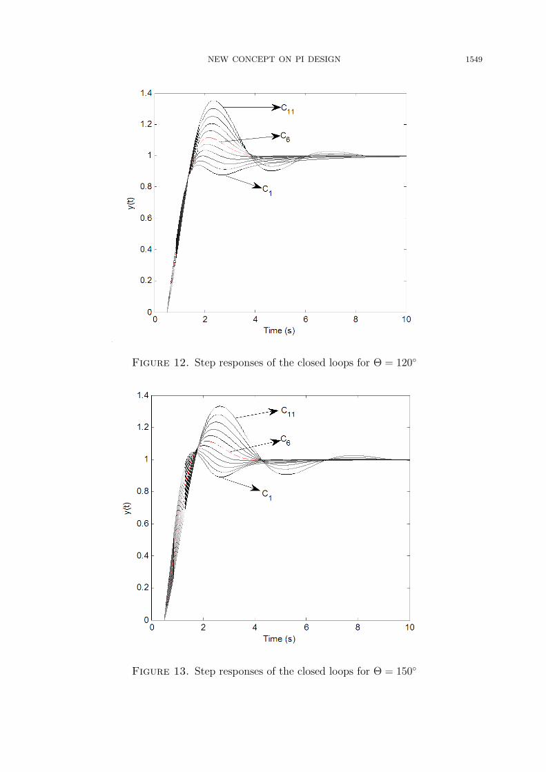
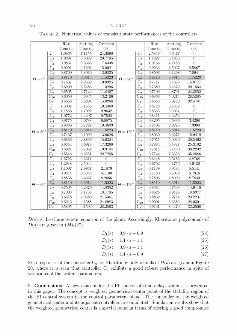
The closed loop step responses are illustrated in Figures 8-13, for the controllers given inTable 1. The aims of the controllers minimize the transient state response performances.The performances are rise time, settling time and overshoot. Numerical values of theseperformances of the closed loops are given in Table 2 for comparison.It can be seen from Figures 8-13 and Table 2 that when the controllers are changed from

C1 to C11 for all values of angle Θ, controller C6 provides a good compromise betweenthe rise time, settling time and overshoot performances. Since this result is illustrated

NEW CONCEPT ON PI DESIGN 1547

Figure 8. Step responses of the closed loops for Θ = 0◦

Figure 9. Step responses of the closed loops for Θ = 30◦

1548 C. ONAT

Figure 10. Step responses of the closed loops for Θ = 60◦

Figure 11. Step responses of the closed loops for Θ = 90◦

NEW CONCEPT ON PI DESIGN 1549

Figure 12. Step responses of the closed loops for Θ = 120◦

Figure 13. Step responses of the closed loops for Θ = 150◦

1550 C. ONAT

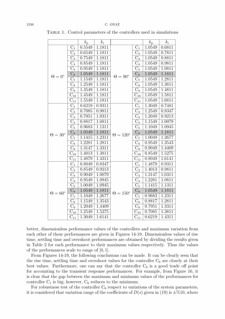
Table 1. Control parameters of the controllers used in simulations

kp ki kp ki

Θ = 0◦

C1 0.5549 1.1811

Θ = 90◦

C1 1.0549 0.6811C2 0.6549 1.1811 C2 1.0549 0.7811C3 0.7549 1.1811 C3 1.0549 0.8811C4 0.8549 1.1811 C4 1.0549 0.9811C5 0.9549 1.1811 C5 1.0549 1.0811C6 1.0549 1.1811 C6 1.0549 1.1811C7 1.1549 1.1811 C7 1.0549 1.2811C8 1.2549 1.1811 C8 1.0549 1.3811C9 1.3549 1.1811 C9 1.0549 1.4811C10 1.4549 1.1811 C10 1.0549 1.5811C11 1.5549 1.1811 C11 1.0549 1.6811

Θ = 30◦

C1 0.6219 0.9311

Θ = 120◦

C1 1.3049 0.7481C2 0.7085 0.9811 C2 1.2549 0.8347C3 0.7951 1.0311 C3 1.2049 0.9213C4 0.8817 1.0811 C4 1.1549 1.0079C5 0.9683 1.1311 C5 1.1049 1.0945C6 1.0549 1.1811 C6 1.0549 1.1811C7 1.1415 1.2311 C7 1.0049 1.2677C8 1.2281 1.2811 C8 0.9549 1.3543C9 1.3147 1.3311 C9 0.9049 1.4409C10 1.4013 1.3811 C10 0.8549 1.5275C11 1.4879 1.4311 C11 0.8049 1.6141

Θ = 60◦

C1 0.8049 0.8347

Θ = 150◦

C1 1.4879 0.9311C2 0.8549 0.9213 C2 1.4013 0.9811C3 0.9049 1.0079 C3 1.3147 1.0311C4 0.9549 1.0945 C4 1.2281 1.0811C5 1.0049 1.0945 C5 1.1415 1.1311C6 1.0549 1.1811 C6 1.0549 1.1811C7 1.1049 1.2677 C7 0.9683 1.2311C8 1.1549 1.3543 C8 0.8817 1.2811C9 1.2049 1.4409 C9 0.7951 1.3311C10 1.2549 1.5275 C10 0.7085 1.3811C11 1.3049 1.6141 C11 0.6219 1.4311

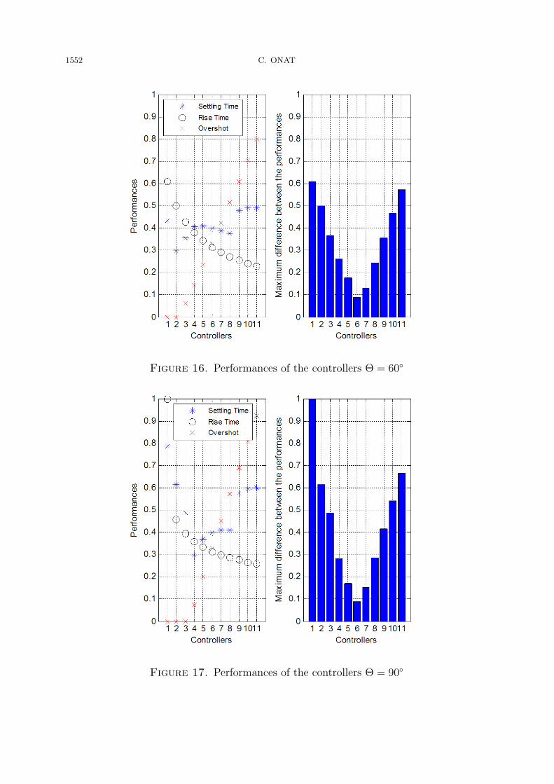
better, dimensionless performance values of the controllers and maximum variation fromeach other of these performances are given in Figures 14-19. Dimensionless values of risetime, settling time and overshoot performances are obtained by dividing the results givenin Table 2 for each performance to their maximum values respectively. Thus the valuesof the performances scale to range of [0, 1].From Figures 14-19, the following conclusions can be made. It can be clearly seen that

the rise time, settling time and overshoot values for the controller C6 are closely at theirbest values. Furthermore, one can say that the controller C6 is a good trade off pointfor accounting to the transient response performances. For example, from Figure 16, itis clear that the gap between the maximum and minimum values of the performances forcontroller C1 is big; however, C6 reduces to the minimum.For robustness test of the controller C6 respect to variations of the system parameters,

it is considered that variation range of the coefficients ofD(s) given in (19) is ±%10, where

NEW CONCEPT ON PI DESIGN 1551

Figure 14. Performances of the controllers Θ = 0◦

Figure 15. Performances of the controllers Θ = 30◦

1552 C. ONAT

Figure 16. Performances of the controllers Θ = 60◦

Figure 17. Performances of the controllers Θ = 90◦

NEW CONCEPT ON PI DESIGN 1553

Figure 18. Performances of the controllers Θ = 120◦

Figure 19. Performances of the controllers Θ = 150◦

1554 C. ONAT

Table 2. Numerical values of transient state performances of the controllers

RiseTime (s)

SettlingTime (s)

Overshot(%)

RiseTime (s)

SettlingTime (s)

Overshot(%)

Θ = 0◦

C1 1.0865 7.1155 24.3890

Θ = 90◦

C1 2.5846 6.6477 0C2 1.0391 6.6089 20.7785 C2 1.1827 5.1936 0C3 0.9861 5.6365 17.6438 C3 1.0156 4.1186 0C4 0.9291 4.1206 15.0021 C4 0.9233 2.5037 2.5867C5 0.8700 3.8030 12.9235 C5 0.8596 3.1298 7.0941C6 0.8110 3.3914 11.5223 C6 0.8110 3.3914 11.5223C7 0.7537 2.9662 10.8925 C7 0.7717 3.4663 15.8777C8 0.6999 3.5486 11.0296 C8 0.7389 3.4572 20.1654C9 0.6505 3.7124 11.8407 C9 0.7109 4.8701 24.3852C10 0.6059 3.6935 13.2106 C10 0.6866 5.0214 28.5285C11 0.5663 3.6304 15.0266 C11 0.6653 5.0726 32.5781

Θ = 30◦

C1 1.3031 5.1586 10.4360

Θ = 120◦

C1 0.8748 6.7852 0C2 1.1863 4.7992 9.9632 C2 0.8555 5.5057 0C3 1.0772 4.4397 9.7522 C3 0.8411 4.3253 0C4 0.9775 4.0788 9.8875 C4 0.8295 3.6896 3.4298C5 0.8886 3.7227 10.4603 C5 0.8196 2.9275 7.3300C6 0.8110 3.3914 11.5223 C6 0.8110 3.3914 11.5223C7 0.7437 3.1099 13.0626 C7 0.8030 3.6271 15.9419C8 0.6856 2.8869 15.0224 C8 0.7955 5.0060 20.5462C9 0.6354 3.6978 17.3266 C9 0.7884 5.5387 25.3102C10 0.5921 3.7062 19.9104 C10 0.7814 5.7480 30.2202C11 0.5546 3.6551 22.7205 C11 0.7744 7.5356 35.2686

Θ = 60◦

C1 1.5725 3.6611 0

Θ = 150◦

C1 0.6448 5.5182 4.8768C2 1.2918 2.5044 0 C2 0.6792 4.1756 4.9130C3 1.1097 2.9957 2.1879 C3 0.7139 3.9484 5.5141C4 0.9814 3.4348 5.1180 C4 0.7480 3.7008 6.7816C5 0.8856 3.4627 8.2666 C5 0.7806 2.8909 8.7840C6 0.8110 3.3914 11.5223 C6 0.8110 3.3914 11.5223C7 0.7505 3.2870 14.8352 C7 0.8384 3.7509 14.9110C8 0.7003 3.1756 18.1785 C8 0.8626 3.9486 18.8377C9 0.6578 4.0589 21.5361 C9 0.8832 5.9754 23.2231C10 0.6212 4.1588 24.8983 C10 0.9001 6.3389 28.0301C11 0.5895 4.1593 28.2593 C11 0.9131 8.4470 33.2506

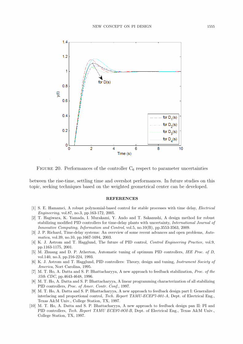
D(s) is the characteristic equation of the plant. Accordingly, Kharitonov polynomials ofD(s) are given in (24)-(27).

D1(s) = 0.9 · s+ 0.9 (24)

D2(s) = 1.1 · s+ 1.1 (25)

D3(s) = 0.9 · s+ 1.1 (26)

D4(s) = 1.1 · s+ 0.9 (27)

Step responses of the controller C6 for Kharitonov polynomials of D(s) are given in Figure20, where it is seen that controller C6 exhibits a good robust performance in spite ofvariations of the system parameters.

5. Conclusions. A new concept for the PI control of time delay systems is presentedin this paper. The concept is weighted geometrical center point of the stability region ofthe PI control system in the control parameters plane. The controller on the weightedgeometrical center and its adjacent controllers are simulated. Simulation results show thatthe weighted geometrical center is a special point in terms of offering a good compromise

NEW CONCEPT ON PI DESIGN 1555

Figure 20. Performances of the controller C6 respect to parameter uncertainties

between the rise-time, settling time and overshot performances. In future studies on thistopic, seeking techniques based on the weighted geometrical center can be developed.

REFERENCES

[1] S. E. Hamamci, A robust polynomial-based control for stable processes with time delay, ElectricalEngineering, vol.87, no.3, pp.163-172, 2005.

[2] T. Hagiwara, K. Yamada, I. Murakami, Y. Ando and T. Sakanushi, A design method for robuststabilizing modified PID controllers for time-delay plants with uncertainty, International Journal ofInnovative Computing, Information and Control, vol.5, no.10(B), pp.3553-3563, 2009.

[3] J. P. Richard, Time-delay systems: An overview of some recent advances and open problems, Auto-matica, vol.39, no.10, pp.1667-1694, 2003.

[4] K. J. Astrom and T. Hagglund, The future of PID control, Control Engineering Practice, vol.9,pp.1163-1175, 2001.

[5] M. Zhuang and D. P. Atherton, Automatic tuning of optimum PID controllers, IEE Proc. of D,vol.140, no.3, pp.216-224, 1993.

[6] K. J. Astrom and T. Hagglund, PID controllers: Theory, design and tuning, Instrument Society ofAmerica, Nort Carolina, 1995.

[7] M. T. Ho, A. Datta and S. P. Bhattacharyya, A new approach to feedback stabilization, Proc. of the35th CDC, pp.4643-4648, 1996.

[8] M. T. Ho, A. Datta and S. P. Bhattacharyya, A linear programming characterization of all stabilizingPID controllers, Proc. of Amer. Contr. Conf., 1997.

[9] M. T. Ho, A. Datta and S. P. Bhattacharyya, A new approach to feedback design part I: Generalizedinterlacing and proportional control, Tech. Report TAMU-ECEP7-001-A, Dept. of Electrical Eng.,Texas A&M Univ., College Station, TX, 1997.

[10] M. T. Ho, A. Datta and S. P. Bhattacharyya, A new approach to feedback design pan II: PI andPID controllers, Tech. Report TAMU ECE97-0OI-B, Dept. of Electrical Eng., Texas A&M Univ.,College Station, TX, 1997.

1556 C. ONAT

[11] N. Munro and M. T. Soylemez, Fast calculation of stabilizing PID controllers for uncertain parametersystems, Proc. of Symposium on Robust Control, Prague, 2000.

[12] M. T. Soylemez, N. Munro and H. Baki, Fast calculation of stabilizing PID controllers, Automatica,vol.39, pp.121-126, 2003.

[13] N. Tan and D. P. Atherton, Feedback stabilization using the Hermite-Biehler theorem, InternationalCon. on the Control of Industrial Processes, Newcastle, UK, 1999.

[14] J. Ackermann and D. Kaesbauer, Design of robust PID controllers, European Control Conference,pp.522-527, 2001.

[15] Z. Shatiei and A. T. Shenton, Frequency domain design of PID controllers for stable and unstablesystems with time delay, Auromotica, vol.33, pp.2223-2232, 1997.

[16] Y. J. Huang and Y. J. Wang, Robust PID tuning strategy for uncertain plants based on theKharitonov theorem, ISA Transactions, vol.39, pp.419-431, 2000.

[17] N. Tan, I. Kaya and D. P. Atherton, Computation of stabilizing PI and PID controllers, IEEEConference on Control Applications, Istanbul, Turkey, 2003.

[18] Y. J. Wang, Graphical computation of gain and phase margin specifications-oriented robust PIDcontrollers for uncertain systems with time-varying delay, Journal of Process Control, vol.21, pp.475-488, 2011.

[19] C. Onat, S. E. Hamamci and S. Obuz, A practical PI tuning approach for time delay systems, IFAC,Boston, USA, 2012.

[20] S. R. Padma, M. N. Srinivas and M. Chidambaram, A simple method of tuning PID controllers forstable and unstable FOPTD systems, Computers and Chemical Engineering, vol.28, pp.2201-2218,2004.

[21] S. Majhi, On-line PI control of stable processes, Journal of Process Control, vol.15, pp.859-867, 2005.