A new analysis of variability and predictability of

INTERNATIONAL JOURNAL OF CLIMATOLOGY

Int. J. Climatol. 24: 1509–1530 (2004)

Published online in Wiley InterScience (www.interscience.wiley.com). DOI: 10.1002/joc.1062

A NEW ANALYSIS OF VARIABILITY AND PREDICTABILITYOF SEASONAL RAINFALL OF CENTRAL

SOUTHERN AFRICA FOR 1950–94

DAVISON MWALE,a THIAN YEW GANa,* and SAMUEL S. P. SHENb

a Department of Civil Engineering, University of Alberta, Edmonton, Alberta, Canadab Department of Mathematics, University of Alberta, Edmonton, Alberta, Canada

Received 15 June 2003Revised 28 April 2004Accepted 28 April 2004

ABSTRACT

Using wavelet analysis and wavelet-based empirical orthogonal function analysis on scale-averaged-wavelet power andindividual scale power, we identified the non-stationary sea-surface temperature (SST) fields of the South Atlantic andIndian Oceans that are associated with coherent regions of rainfall variability in central southern Africa (CSA). Thedominant mode of CSA rainfall is out of phase between the coastal areas and the centre of CSA and has been decreasingconsistently since 1970. The frequencies associated with this mode are between 2–2.4 and 5.6–8 years. The Benguelaocean current SSTs form the dominant spatial pattern of the South Atlantic Ocean, and the Brazil and Guinea oceancurrent SSTs form the second leading mode. The Benguela spatial patterns were found to migrate seasonally betweenAfrica’s west coast and South America’s east coast. The northern Indian Ocean SST forms the leading mode of variability,followed by the south Indian Ocean SST. Using predictor fields identified from both oceans, we achieved encouragingresults of predicted CSA rainfall using a non-linear statistical teleconnection artificial neural network–genetic algorithmmodel. At 3 month lead time, correlations of between 0.8 and 0.9, root-mean-square errors of between 0.4 and 0.9and Hansen Kuipers skill scores of between 0.4 and 0.8 were obtained between observed and predicted CSA rainfall.Copyright 2004 Royal Meteorological Society.

KEY WORDS: wavelet empirical orthogonal function analysis; scale-averaged wavelet power; seasonal rainfall; central southern Africa;sea surface temperature; Indian Ocean; Atlantic Ocean; genetic algorithm–neural network

1. INTRODUCTION

Wavelet transformation, a process of decomposing a time series into frequency and energy components overtime, is now an established analysis tool for non-stationary processes. Wavelet transformations have beensuccessfully applied to climate characteristics analysis, such as streamflow characterization (Smith et al.,1998), temporal structure of the southern oscillation (Wang and Wang, 1996) and interannual temperatureevents and shifts in global temperature (Park and Mann, 2000). Results from these and other studies haveshown that wavelets are capable of locating irregularly distributed multi-scale features of climate elements inspace and time (Smith et al., 1998).

Among the physical elements of our climate system, rainfall is very complex and exhibits considerablespatial, temporal and frequency variability (Basalirwa, 1995; Shen et al., 2001). Problems of quantifyingrainfall variability with respect to climatic elements, such as sea-surface temperature (SST), have been asubject of numerous studies (e.g. Mason, 1995; Mutai et al., 1998; Reason and Mulenga, 1999). Many paststudies have applied a combination of time domain multivariate statistics, such as harmonic analysis, Fourieranalysis, linear regressions and cross-correlations, to climate data to determine relationships between and

* Correspondence to: Thian Yew Gan, Department of Civil and Environmental Engineering, University of Alberta, Edmonton, AlbertaT6G 2G7, Canada; e-mail: [email protected]

Copyright 2004 Royal Meteorological Society

1510 D. MWALE, T. YEW GAN AND SAMUEL S. P. SHEN

among the climate elements. A common and well-recognized shortcoming of these approaches has been theassumption that climate data are stationary and linear, criteria that few data sets from natural phenomenasatisfy (Huang et al., 1998).

With an unstable relationship between rainfall in southern Africa and SST in the surrounding oceans inrecent years (Landman and Mason, 1999) and a consistent pattern of declining runoff of most rivers in southernAfrica after 1970 (Fanta et al., 2001), one of the major challenges for climatologists and hydrologists hasbeen to predict the nature of the variability in space and time.

Recent research has made progress in providing evidence of relationships between rainfall variability anda number of atmospheric and oceanic variables for parts of southern Africa (e.g. Mason, 1995; Jury, 1996;Reason and Mulenga, 1999). From developments in long-range forecast models utilizing SST and otherpredictors, one would have hoped that these developments would offer countries within the southern Africanregion the prospect of managing climate variability rather than always being surprised victims of unexpectedextreme events, such as droughts (e.g. Barnston et al., 1996; Landman and Tennant, 2000; Landman et al.,2001). However, there are still difficulties associated with rainfall prediction at seasonal lead time (Mason,1997), and this seems more so in recent times. For example, the Indian Meteorological Department usedmodels based on empirical relationships between monsoon and worldwide climate predictors with moderatesuccess in the past (Webster et al., 2002), but forecast skill after the 1980s has been low (Mason, 1997).Similarly, it seems that the skill for forecasting the frequencies of North Atlantic storms also faced difficultiesafter 1989 (Mason, 1997).

Decreased predictability has been associated with a combination of non-stationarity (interannual andinterdecadal scales) of the ocean–atmosphere system, non-linearity of the ocean–atmosphere interactionand model inadequacies (Allan et al., 1995; Webster et al., 2002). In other words, empirical forecasts haveto contend with the spectre of statistical non-stationarity (Webster et al., 2002) in understanding climatevariability and identifying relationships between climate elements to avoid driving predictor models withambiguous input data that result in compromised prediction skill (Jury and Engert, 1999; Shen et al.,2001).

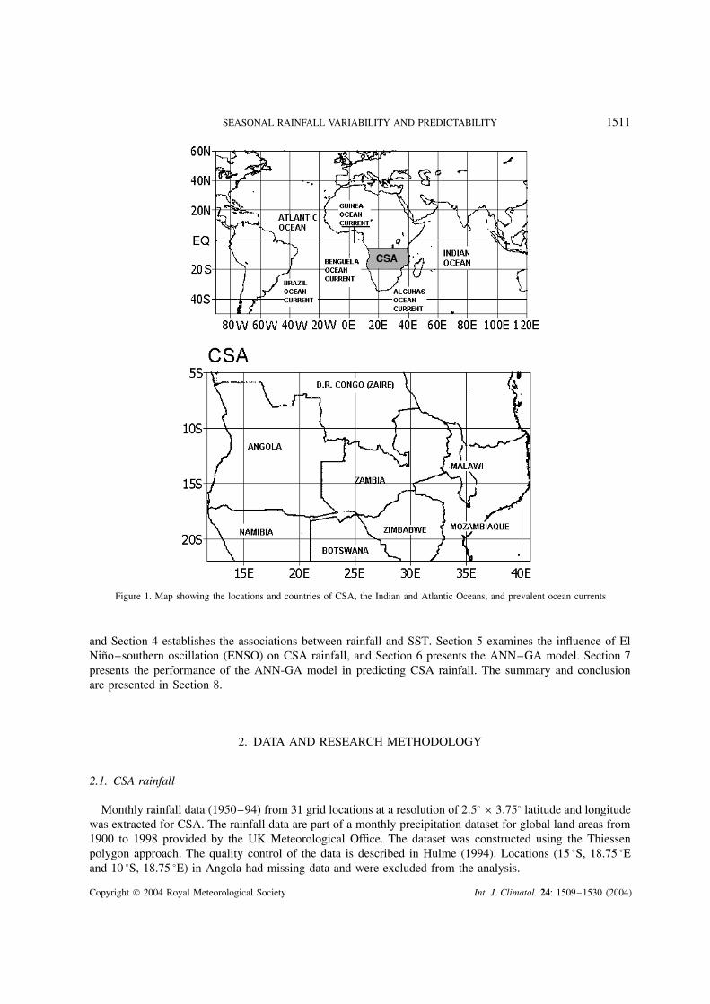
Like the rest of southern Africa, rainfall in central southern Africa (CSA; 10–20 °S, 12–42 °E), Figure 1,occurs during Southern Hemisphere summer, which commences in October and ends in March. CSA hasalso suffered from repeated droughts in recent years (e.g. BBC, 2002a,b). The sudden outburst of droughtsbetween 1991 and 2002 compared with periods prior to 1991 is a good example of the non-stationarity ofthe CSA climate.

A few possible ways to overcome the problem of non-stationarity include wavelet analysis and wavelet-based empirical orthogonal function (WEOF) analysis, empirical mode decomposition with Hilbert spectralanalysis (EMD-HSA), and EMD-HSA-based EOF analysis. Here, we use wavelet analysis and WEOF analysisto study the spatial, temporal and frequency regimes of CSA rainfall, Indian and South Atlantic Ocean SSTvariability, and their associations. WEOF analysis has previously been used in chemical process monitoring(e.g. Bakshi, 1989), but, as far as we know, this is the first time WEOF analysis has been used to analysethe variability of rainfall and SST in the surrounding oceans. The specific research objectives of this studyare as follows:

1. To identify and analyse the dominant, non-stationary, spatial, temporal and frequency regimes of the CSArainfall and SST fields of the South Atlantic and the Indian Ocean SST, and, by identifying SST fields ofboth oceans relevant to CSA rainfall, their possible association.

2. Use the relevant predictor fields obtained from the foregoing to drive a non-linear, artificial neural networkcalibrated by a genetic algorithm (ANN–GA) to predict CSA rainfall at seasonal time scales (i.e. 3 monthlead time).

By combining the analysis techniques of wavelet, WEOF, and the statistical forecasting method, ANN–GA,we expect to understand the non-stationarity of CSA rainfall and SST better, and also to improve the seasonalprediction of CSA rainfall using statistical methods. The paper is organized as follows: Section 2 discusses thedata and the methodology of analysis used in this paper. Section 3 discusses SST and CSA rainfall variability,

Copyright 2004 Royal Meteorological Society Int. J. Climatol. 24: 1509–1530 (2004)

SEASONAL RAINFALL VARIABILITY AND PREDICTABILITY 1511

Figure 1. Map showing the locations and countries of CSA, the Indian and Atlantic Oceans, and prevalent ocean currents

and Section 4 establishes the associations between rainfall and SST. Section 5 examines the influence of ElNino–southern oscillation (ENSO) on CSA rainfall, and Section 6 presents the ANN–GA model. Section 7presents the performance of the ANN-GA model in predicting CSA rainfall. The summary and conclusionare presented in Section 8.

2. DATA AND RESEARCH METHODOLOGY

2.1. CSA rainfall

Monthly rainfall data (1950–94) from 31 grid locations at a resolution of 2.5° × 3.75° latitude and longitudewas extracted for CSA. The rainfall data are part of a monthly precipitation dataset for global land areas from1900 to 1998 provided by the UK Meteorological Office. The dataset was constructed using the Thiessenpolygon approach. The quality control of the data is described in Hulme (1994). Locations (15 °S, 18.75 °Eand 10 °S, 18.75 °E) in Angola had missing data and were excluded from the analysis.



2.2. SST of Indian and Atlantic Oceans

Monthly SST anomaly grid data at 5° × 5° latitude and longitude resolution was extracted from 290 gridlocations in the Indian Ocean (20 °N–40 °S, 40–105 °E) and Atlantic Ocean (10 °N–40 °S, 55 °W–10 °E); seeFigure 1. The SST datasets were 48 years long (1950–97) and were transformed into seasonal and annualdata by computing 3 month (i.e. January–March (JFM), April–June (AMJ), July–September (JAS) andOctober–December (OND)) and 12 month averages respectively. The SST dataset is part of MOHSST6, ahistorical global dataset of mean monthly global SST anomalies with respect to the 1961–90 normals providedby the UK Meteorological Office.

2.3. Wavelet analysis

A brief outline of wavelet transformation is given herein (see Torrence and Compo (1998) for details).Wavelets are a set of limited duration waves, also called daughter wavelets, because they are formed bydilations and translations of a single prototype wavelet function �(t), where t is real valued, called the basicor mother wavelet (Castleman, 1996). The mother wavelet is designed to oscillate as a wave and requiredto span an area that sums to zero, and to die out rapidly to zero as t tends to infinity in order to satisfy the‘admissibility’ condition:∫

�(t) dt = 0 (1)

A set of wavelets can be generated by translating and scaling the basic wavelet as

�a,b(t) = 1√a�

(t − b

a

)(2)

where the scale (width) of the wavelet and translated position along the t-axis (usually the x-axis in the x –y

plane) are a and b respectively. When a is increased, the wavelet width increases and a convolution of atime series with the wavelet isolates the low-frequency part of the time series. Conversely, if a is decreased,the wavelet width decreases and the high-frequency components of the time series can be isolated. Thismeans that, if the scale is continuously varied along the translation b, a picture can be constructed depictinghow the isolated components of the time series at each frequency vary with the time. Associated with eachfrequency are numerical coefficients referred to as the energy of the wavelet spectrum, which represent howwell the wavelet matches with the time series. The parameters a and b in Equation (2) are real and a, alwayspositive, may range over a continuous or a discrete set. The quantity a−1/2 in Equation (2) is an energynormalization term, which ensures that the energies of the mother and daughter wavelets remain the sameover all scales, making it possible to compare wavelet transforms of one time series with another directly(Torrence and Compo, 1998). The wavelet transform of a real signal X(t) with respect to the mother waveletis a convolution integral given as

W(b, a) = 1√a

∫ T

0X(t)�∗

(t − b

a

)dt (3)

where �∗ is the complex conjugate of �. In Equation (3), W (b, a) is a wavelet spectrum, a matrix of energycoefficients of the decomposed time series X(t). The energy coefficients also represent the magnitude ofvariance (variability) of coefficients at each scale a and location in time t . A faster and much more efficientway to compute the wavelet transform is done in the Fourier space using the Fourier transform of a discretetime series X(t) as

Wt(a) =T∑

k=0

X�∗(sωk)eiωknδt (4)



where the caret symbolizes Fourier transform, k is the frequency index (0, . . . , T ) and �(sωk) is the Fouriertransform of the wavelet function. The wavelet spectrum was computed using discrete scales in fractionalpowers of two:

sj = s02jδj (5)

where s0 is twice the sampling rate, j = (0, 1, . . . , 20), and δj is the step size (e.g. 0.25). The wavelettransform of a time series contains a wealth of information at each time scale. This information can also becondensed over a range of scales or time in order to be conveniently used for multivariate analysis. Two wayssuggested by Torrence and Compo (1998) are (1) time-integrated variance of energy coefficients at everyscale to construct global wavelet power:

W2t (a) = 1

T

T −1∑t=0

|Wt(a)|2 (6)

and (2) scale- (band-limited) integrated variance of energy coefficients over time to construct the scale-averaged wavelet power (SAWP):

W 2t = δj δt

Cδ

j2∑j=j1

|Wt(aj )|2aj

(7)

where Cδ is the reconstruction factor that takes on values depending on the mother wavelet used, δj is afactor for scale averaging, j1 and j2 are scales over which the averaging takes place, and δt is the samplingperiod (Torrence and Compo, 1998). The global wavelet spectrum depicts dominant oscillations present in atime series, and the local wavelet power shows how the dominant oscillations vary with time. To computethe wavelet power for this study, the Morlet wavelet (k = 6) was used because its structure resembles thatof a rainfall time series. It is made up of a harmonic wave modulated by a Gaussian envelope:

�(t) = π1/4ei6te−t2/2 (8)

2.4. WEOF analysis

Empirical orthogonal function (EOF) analysis of raw data fields has been widely used for the analysis ofspatial and temporal variability of physical fields to identify objectively the spatially uncorrelated modes ofvariability of a given field (Kutzbach, 1967; Mason, 1995; Venegas et al., 1997). In this study, EOF analysisis applied to the SAWP. To distinguish the EOF of raw data from that of the SAWP, the latter is calleda WEOF and its corresponding principal components (PCs) are herein referred to as wavelet PCs (WPCs)to distinguish them from raw data PCs. The time-domain WPCs are obtained by projecting the SAWP ontothe SAWP eigenvectors. Since the WPCs are obtained from the SAWP, they are interpreted as ‘frequencycompacted’ energy variability (Park and Mann, 2000).

To identify and delineate temporal and spatially uncorrelated patterns in the time–frequency plane withcoherent variations at regional scale, we applied WEOF analysis to the SAWP and the individual scale power(ISP) of the SST of the South Atlantic and Indian Ocean and CSA rainfall. Other techniques can be usedin place of WEOF analysis to meet this objective, such as cluster analysis (Wilks, 1995), harmonic analysis(Ntale et al., 2003), etc. However, the skill of the above methods is often difficult to evaluate statistically(Basalirwa, 1995).

3. VARIABILITY OF CSA RAINFALL AND SST IN THE INDIAN AND ATLANTIC OCEANS

3.1. Dominant modes of SST and rainfall variability

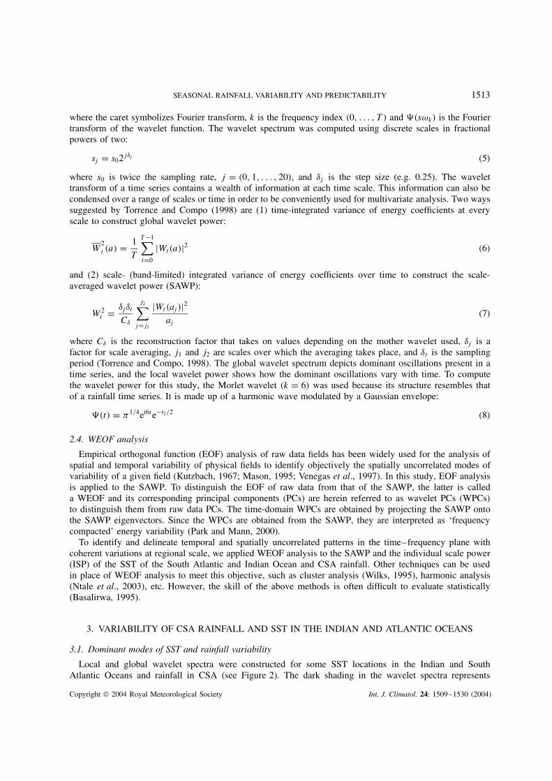
Local and global wavelet spectra were constructed for some SST locations in the Indian and SouthAtlantic Oceans and rainfall in CSA (see Figure 2). The dark shading in the wavelet spectra represents



1950 1955 1960 1965 1970 1975 1980 1985 1990 1995 0 5 10

Time (year) Power (mm2)

32

16

8

4P

erio

d (y

ears

)

1950 1955 1960 1965 1970 1975 1980 1985 1990 1995 0 0.05 0.1

Time (year) Power (DegC2)

32

16

8

4

Per

iod

(yea

rs)

1950 1955 1960 1965 1970 1975 1980 1985 1990 1995 0 0.2 0.4

Time (year) Power (DegC2)

32

16

8

4

Per

iod

(yea

rs)

(a) CSA rainfall

(b) Indian Ocean SST

(c) Atlantic Ocean SST

Figure 2. Examples of local and global wavelet spectra constructed for (a) the CSA rainfall, (b) the Indian Ocean, and (c) the AtlanticOcean SST. The variation of power is suppressed at the beginning and end of each wavelet spectrum, since zeros used to pad both endsof the time series decrease the power. These affected areas are located outside the line with dots, which represents the COI. The darkshading in the wavelet spectra represents areas that contain power significant at the 95% confidence level of a red-noise process. In theglobal wavelet spectrum, the dotted curve represents the 95% confidence level, and peaks above the curve are considered statistically

significant

areas that contain power (or energy) significant at the 95% confidence level of a red-noise process. Theline with dots through the wavelet spectra delineates the cone of influence (COI). Since the length ofthe data used is finite, the ends of the time series were padded with zeros to bring the total length ofthe time series to the next-higher power of two, e.g. 512, 1024, etc. This facilitated the computation ofwavelet power at larger scales and also speeded up the computation of wavelet transformation. However,padding the ends of time series with zeros introduces discontinuities at the endpoints of the time seriesand, as one goes towards larger scales, the amplitude near the edges decreases as more zeros enter theanalysis. Therefore, at the beginning and end of the SAWP time series, the variation of power is generallysuppressed.

There is appreciable power in the CSA rainfall and SST data at both high and low frequencies(Figure 2). However, the variation of rainfall and SST data is clearly dominated by peaks whoseperiods were between 2 and 8 years, i.e. the ENSO band. The concentration of energy within theseperiods is clearly visible as statistically significant peaks in the global wavelet spectra. Hence, forthis study, the periods of between 2 and 8 years were chosen for the analysis of rainfall and SSTvariability.



3.2. CSA rainfall variability

We applied WEOF analysis to the SAWP of the 31 rainfall grid stations and retained two leading WPCs,which individually explained 24% and 17% of the total SAWP variance. The WEOF analysis was basedon the correlation matrix, and the spatial distributions of the WPCs are shown in form of the correlationcoefficient between WPCs and the 31 SAWP time series (see Figure 3). The leading spatial patterns show theregional variation of the SAWP. The discarded WPCs mainly described the SAWP variations of local features(e.g. the Zambezi River basin and the Lake Malawi basin). Since this paper analyses the regional variationof the SAWP and its relationship to SST, the third and higher WPCs are not discussed further.

WPC1 displays an out-of-phase relationship between the central CSA and the coastal regions along theeast and west coasts. Statistically significant negative correlations between WPC1 and the SAWP occur alongthe coastal regions of Angola. Large positive correlations are evident over all of Zambia, Malawi, northernZimbabwe and parts of Mozambique. WPC2 displays an out-of-phase relationship that extends diagonallyfrom the northwest to the southeast of CSA. Statistically significant correlations occur in northeast Zimbabweand central Mozambique.

The temporal variability of the WPCs is shown in Figure 3(c). The variance of WPC1 was high between1950 and 1980, but decreased significantly between 1981 and 1994. Since WPC1 is positively correlatedto central CSA (Zambia, Malawi, Zimbabwe and northern Mozambique), rainfall in these regions has beenon the decline for over three decades (i.e. 1970–94). These results are consistent with findings of Fantaet al. (2001), who found that streamflow runoff consistently declined between the 1970s and 1997. Hence,the time-domain WPCs accurately represent the temporal variability of CSA rainfall. Unlike WPC1, WPC2exhibited higher variations throughout the 1950–94 period and shows the diagonal north–south variation ofCSA rainfall.

15E 20E 25E 30E 35E 40E

20S

15S

10S

5S

15E 20E 25E 30E 35E 40E

20S

15S

10S

5S

-6

-4

-2

0

2

4

6

8

Var

ianc

e

WPC1 (30%)WPC2 (22%)

Time (Year)

(c)

(a) 30% (b) 22%

Figure 3. Contour plots of the spatial correlation patterns between (a) WPC1 and (b) WPC2 of the CSA rainfall and the SAWP ofindividual grids at 0.1 contour intervals. The numbers shown above represent the percentage of the total variance explained by eachWPC. The dark areas correspond to correlations significant at the 95% confidence level. The temporal variations of the two WPCs of

CSA rainfall are shown in (c)



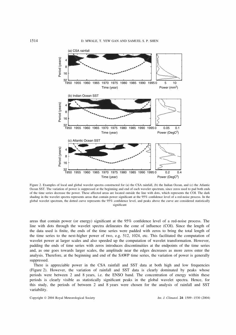
3.3. South Atlantic Ocean SST variability

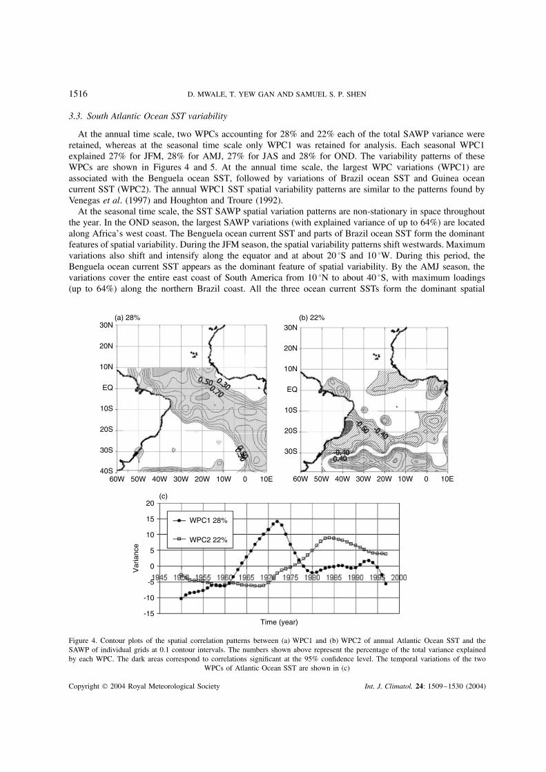
At the annual time scale, two WPCs accounting for 28% and 22% each of the total SAWP variance wereretained, whereas at the seasonal time scale only WPC1 was retained for analysis. Each seasonal WPC1explained 27% for JFM, 28% for AMJ, 27% for JAS and 28% for OND. The variability patterns of theseWPCs are shown in Figures 4 and 5. At the annual time scale, the largest WPC variations (WPC1) areassociated with the Benguela ocean SST, followed by variations of Brazil ocean SST and Guinea oceancurrent SST (WPC2). The annual WPC1 SST spatial variability patterns are similar to the patterns found byVenegas et al. (1997) and Houghton and Troure (1992).

At the seasonal time scale, the SST SAWP spatial variation patterns are non-stationary in space throughoutthe year. In the OND season, the largest SAWP variations (with explained variance of up to 64%) are locatedalong Africa’s west coast. The Benguela ocean current SST and parts of Brazil ocean SST form the dominantfeatures of spatial variability. During the JFM season, the spatial variability patterns shift westwards. Maximumvariations also shift and intensify along the equator and at about 20 °S and 10 °W. During this period, theBenguela ocean current SST appears as the dominant feature of spatial variability. By the AMJ season, thevariations cover the entire east coast of South America from 10 °N to about 40 °S, with maximum loadings(up to 64%) along the northern Brazil coast. All the three ocean current SSTs form the dominant spatial

60W 50W 40W 30W 20W 10W 0 10E40S

30S

20S

10S

EQ

10N

20N

30N

60W 50W 40W 30W 20W 10W 0 10E

30S

20S

10S

EQ

10N

20N

30N

-15

-10

-5

0

5

10

15

20

Var

ianc

e

WPC1 28%

WPC2 22%

Time (year)

(a) 28%

(c)

(b) 22%

Figure 4. Contour plots of the spatial correlation patterns between (a) WPC1 and (b) WPC2 of annual Atlantic Ocean SST and theSAWP of individual grids at 0.1 contour intervals. The numbers shown above represent the percentage of the total variance explainedby each WPC. The dark areas correspond to correlations significant at the 95% confidence level. The temporal variations of the two

WPCs of Atlantic Ocean SST are shown in (c)



50W 40W 30W 20W 10W 0 10E40S

30S

20S

10S

EQ

10N

20N

30N(a) OND 27%

50W 40W 30W 20W 10W 0 10E40S

30S

20S

10S

EQ

10N

20N

30N(b) JFM 28%

50W 40W 30W 20W 10W 0 10E40S

30S

20S

10S

EQ

10N

20N

30N(d) JAS 28%

50W 40W 30W 20W 10W 0 10E40S

30S

20S

10S

EQ

10N

20N

30N(c) AMJ 27%

Figure 5. Contour plots of the spatial correlation patterns between WPC1 of seasonal Atlantic Ocean SST and the SAWP of individualgrids at 0.1 contour intervals for (a) OND, (b) JFM, (c) AMJ, and (d) JAS seasons. The numbers shown above represent the percentageof the total variance explained by each WPC1. The seasonal migration of spatial variability patterns of SST can be seen from (a) to (d)

feature of variability. However, the variability of the Guinea ocean current SST is out of phase with the restof the Atlantic Ocean SST. In the JAS season, the spatial variability patterns begin to shift eastwards towardsthe African coastal areas, with the Benguela as the sole pattern of spatial variability.

The migration of the SAWP spatial variation patterns between South America and Africa is a new findingthat has important implications for understanding both the lagged and simultaneous relationships between SSTin the South Atlantic Ocean and rainfall in South America and CSA, and probably most of sub-Saharan Africa.

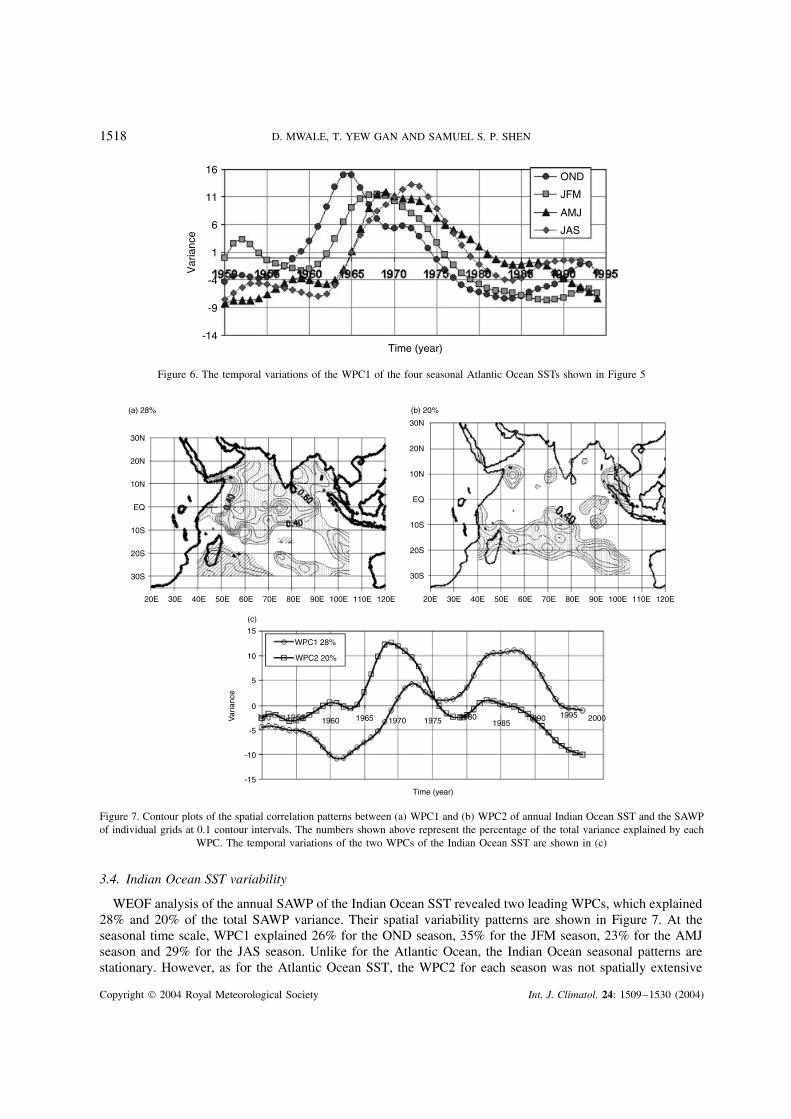
The time-domain WPC for the annual and seasonal SAWP shows large variation between 1950 and 1980,followed by a relatively quiet period between 1980 and 1994, similar to the CSA WPC1 (see Figures 4and 6). SST energy increased (temperature rise) between 1950 and 1972 and was followed by a decreasebetween 1972 and 1980. WPC2 (less variable than WPC1) shows increasing power from 1969 to 1984, witha decrease that started in 1985.



-14

-9

-4

1

6

11

16

Var

ianc

e

Time (year)

OND

JFM

AMJ

JAS

Figure 6. The temporal variations of the WPC1 of the four seasonal Atlantic Ocean SSTs shown in Figure 5

30N

30S

20S

10S

EQ

10N

20N

120E110E100E90E80E70E60E50E40E30E20E

15

5

10

0

-5

-10

-15

Time (year)

Var

ianc

e

30N

30S

20S

10S

EQ

10N

20N

120E110E100E90E80E70E60E50E40E30E20E

WPC1 28%

WPC2 20%

1960 1965 1970 1975 19801985

1990 1995 2000

(a) 28% (b) 20%

(c)

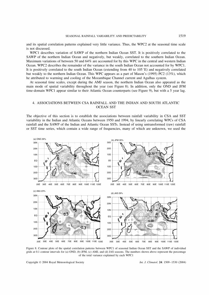
Figure 7. Contour plots of the spatial correlation patterns between (a) WPC1 and (b) WPC2 of annual Indian Ocean SST and the SAWPof individual grids at 0.1 contour intervals. The numbers shown above represent the percentage of the total variance explained by each

WPC. The temporal variations of the two WPCs of the Indian Ocean SST are shown in (c)

3.4. Indian Ocean SST variability

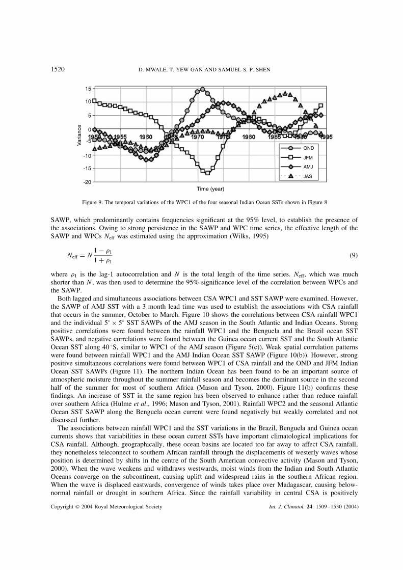
WEOF analysis of the annual SAWP of the Indian Ocean SST revealed two leading WPCs, which explained28% and 20% of the total SAWP variance. Their spatial variability patterns are shown in Figure 7. At theseasonal time scale, WPC1 explained 26% for the OND season, 35% for the JFM season, 23% for the AMJseason and 29% for the JAS season. Unlike for the Atlantic Ocean, the Indian Ocean seasonal patterns arestationary. However, as for the Atlantic Ocean SST, the WPC2 for each season was not spatially extensive



and its spatial correlation patterns explained very little variance. Thus, the WPC2 at the seasonal time scaleis not discussed.

WPC1 describes variation of SAWP of the northern Indian Ocean SST. It is positively correlated to theSAWP of the northern Indian Ocean and negatively, but weakly, correlated to the southern Indian Ocean.Maximum variations of between 50 and 64% are accounted for by this WPC in the central and western IndianOcean. WPC2 describes the remainder of the variance in the south Indian Ocean not accounted for by WPC1.It is positively correlated to the south Indian Ocean (extending from 40 to 105 °E) and negatively correlatedbut weakly to the northern Indian Ocean. This WPC appears as a part of Mason’s (1995) PC2 (13%), whichhe attributed to warming and cooling of the Mozambique Channel current and Agulhas system.

At seasonal time scales, except during the AMJ season, the northern Indian Ocean also appeared as themain mode of spatial variability throughout the year (see Figure 8). In addition, only the OND and JFMtime-domain WPC1 appear similar to their Atlantic Ocean counterparts (see Figure 9), but with a 5 year lag.

4. ASSOCIATIONS BETWEEN CSA RAINFALL AND THE INDIAN AND SOUTH ATLANTICOCEAN SST

The objective of this section is to establish the associations between rainfall variability in CSA and SSTvariability in the Indian and Atlantic Oceans between 1950 and 1994, by linearly correlating WPCs of CSArainfall and the SAWP of the Indian and Atlantic Ocean SSTs. Instead of using untransformed (raw) rainfallor SST time series, which contain a wide range of frequencies, many of which are unknown, we used the

30N

30S

20S

10S

EQ

10N

20N

120E110E100E90E80E70E60E50E40E30E20E 120E110E100E90E80E70E60E50E40E30E20E

30S

30S

20S

10S

0S

10S

20S

(a) OND 26% (b) JFM 35%

120E110E100E90E80E70E60E50E40E30E20E

30N

30S

20S

10S

EQ

10N

20N

(c) AMJ 23%

30N

30S

20S

10S

EQ

10N

20N

120E110E100E90E80E70E60E50E40E30E20E

(d) JAS 29%

Figure 8. Contour plots of the spatial correlation patterns between WPC1 of seasonal Indian Ocean SST and the SAWP of individualgrids at 0.1 contour intervals for (a) OND, (b) JFM, (c) AMJ, and (d) JAS seasons. The numbers shown above represent the percentage

of the total variance explained by each WPC1



15

10

-5

-10

-15

-20

0

5

Time (year)

Var

ianc

e

OND

JFM

AMJ

JAS

Figure 9. The temporal variations of the WPC1 of the four seasonal Indian Ocean SSTs shown in Figure 8

SAWP, which predominantly contains frequencies significant at the 95% level, to establish the presence ofthe associations. Owing to strong persistence in the SAWP and WPC time series, the effective length of theSAWP and WPCs Neff was estimated using the approximation (Wilks, 1995)

Neff = N1 − ρ1

1 + ρ1(9)

where ρ1 is the lag-1 autocorrelation and N is the total length of the time series. Neff, which was muchshorter than N , was then used to determine the 95% significance level of the correlation between WPCs andthe SAWP.

Both lagged and simultaneous associations between CSA WPC1 and SST SAWP were examined. However,the SAWP of AMJ SST with a 3 month lead time was used to establish the associations with CSA rainfallthat occurs in the summer, October to March. Figure 10 shows the correlations between CSA rainfall WPC1and the individual 5° × 5° SST SAWPs of the AMJ season in the South Atlantic and Indian Oceans. Strongpositive correlations were found between the rainfall WPC1 and the Benguela and the Brazil ocean SSTSAWPs, and negative correlations were found between the Guinea ocean current SST and the South AtlanticOcean SST along 40 °S, similar to WPC1 of the AMJ season (Figure 5(c)). Weak spatial correlation patternswere found between rainfall WPC1 and the AMJ Indian Ocean SST SAWP (Figure 10(b)). However, strongpositive simultaneous correlations were found between WPC1 of CSA rainfall and the OND and JFM IndianOcean SST SAWPs (Figure 11). The northern Indian Ocean has been found to be an important source ofatmospheric moisture throughout the summer rainfall season and becomes the dominant source in the secondhalf of the summer for most of southern Africa (Mason and Tyson, 2000). Figure 11(b) confirms thesefindings. An increase of SST in the same region has been observed to enhance rather than reduce rainfallover southern Africa (Hulme et al., 1996; Mason and Tyson, 2001). Rainfall WPC2 and the seasonal AtlanticOcean SST SAWP along the Benguela ocean current were found negatively but weakly correlated and notdiscussed further.

The associations between rainfall WPC1 and the SST variations in the Brazil, Benguela and Guinea oceancurrents shows that variabilities in these ocean current SSTs have important climatological implications forCSA rainfall. Although, geographically, these ocean basins are located too far away to affect CSA rainfall,they nonetheless teleconnect to southern African rainfall through the displacements of westerly waves whoseposition is determined by shifts in the centre of the South American convective activity (Mason and Tyson,2000). When the wave weakens and withdraws westwards, moist winds from the Indian and South AtlanticOceans converge on the subcontinent, causing uplift and widespread rains in the southern African region.When the wave is displaced eastwards, convergence of winds takes place over Madagascar, causing below-normal rainfall or drought in southern Africa. Since the rainfall variability in central CSA is positively



30N

30S

20S

10S

EQ

10N

20N

40S50W 10W 020W30W40W 10E

(a)

120E110E100E90E80E70E60E50E40E30E20E

30N

30S

20S

10S

10N

20N

EQ

(b)

Figure 10. Plots showing the spatial correlation patterns between WPC1 of CSA rainfall and individual 5° × 5° AMJ SST SAWP timeseries of the (a) Atlantic Ocean and (b) Indian Ocean. The areas inside the dotted line correspond to ocean zones with correlations

greater than 0.5. Data from these delineated zones were later used to predict the CSA rainfall

30N

30S

20S

10S

EQ

10N

20N

120E110E100E90E80E70E60E50E40E30E20E

(a)

30N

30S

20S

10S

EQ

10N

20N

120E110E100E90E80E70E60E50E40E30E20E

(b)

Figure 11. Contour plots at 0.1 contour intervals of the spatial correlation patterns between WPC1 of CSA rainfall and the SAWP ofthe Indian Ocean for (a) OND and (b) JFM seasons. During JFM, the latter half of the CSA rainy season, it seems that the dominant

source of moisture supply to CSA’s rainfall comes from the central Indian Ocean



associated with SST in the Brazil and Benguela ocean currents, warming in these ocean basins results inincreased rainfall in central CSA and vice versa for the coastal areas.

5. INFLUENCE OF ENSO ON CSA RAINFALL VARIABILITY

In this section we examine how the ENSO signal affects the spatial and temporal variability of CSA rainfall.The wavelet and global spectra showed that most of the power of the rainfall and SST lies within the ENSOband (i.e. 2–8 year cycles band). In addition, past studies of rainfall of some countries in CSA (e.g. northernNamibia, Zimbabwe and Botswana) found a number of cycles in the rainfall in the 2–8 year range (i.e. 2,2.3, 2.8, 3.5, 6.7 and 7 years) and others at 11 years and 18–20 years (e.g. Nicholson, 1986; Ropelewski andHalpert, 1987; Mason and Tyson, 2000). In this paper, the spatial and temporal variability of the power (orenergy) at each of these cycles is examined against the temporal evolution of ENSO episodes between 1950and 1994.

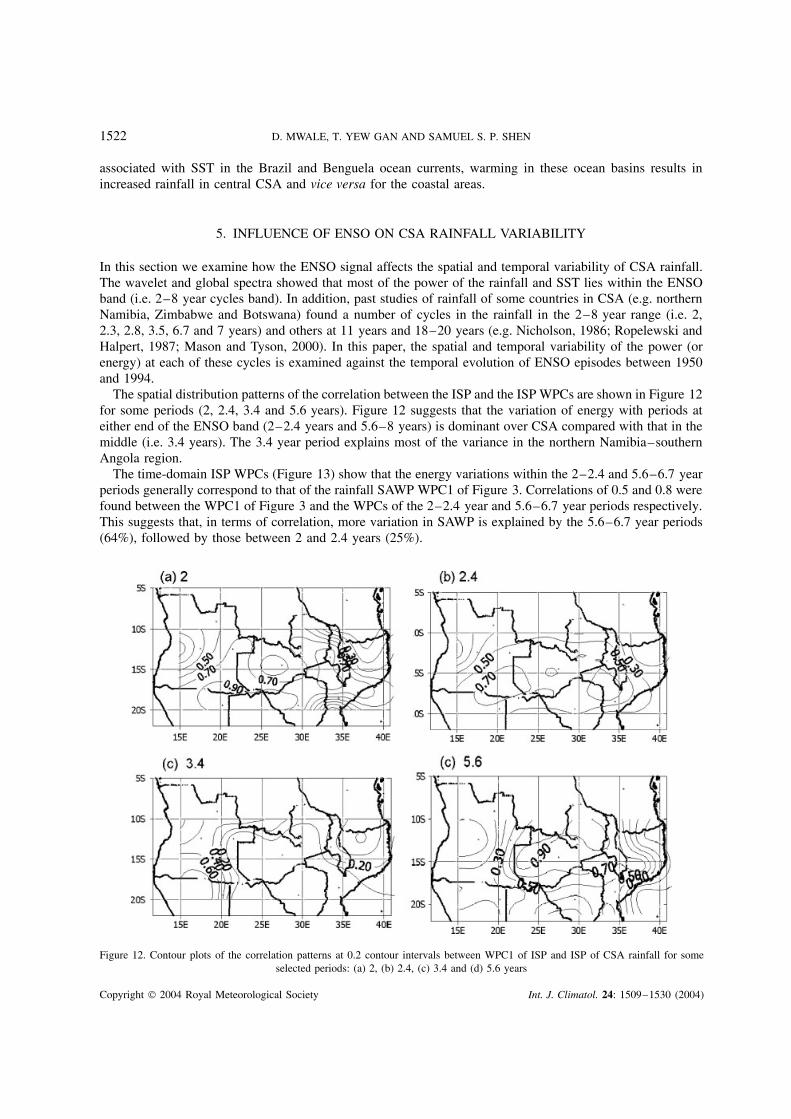
The spatial distribution patterns of the correlation between the ISP and the ISP WPCs are shown in Figure 12for some periods (2, 2.4, 3.4 and 5.6 years). Figure 12 suggests that the variation of energy with periods ateither end of the ENSO band (2–2.4 years and 5.6–8 years) is dominant over CSA compared with that in themiddle (i.e. 3.4 years). The 3.4 year period explains most of the variance in the northern Namibia–southernAngola region.

The time-domain ISP WPCs (Figure 13) show that the energy variations within the 2–2.4 and 5.6–6.7 yearperiods generally correspond to that of the rainfall SAWP WPC1 of Figure 3. Correlations of 0.5 and 0.8 werefound between the WPC1 of Figure 3 and the WPCs of the 2–2.4 year and 5.6–6.7 year periods respectively.This suggests that, in terms of correlation, more variation in SAWP is explained by the 5.6–6.7 year periods(64%), followed by those between 2 and 2.4 years (25%).

Figure 12. Contour plots of the correlation patterns at 0.2 contour intervals between WPC1 of ISP and ISP of CSA rainfall for someselected periods: (a) 2, (b) 2.4, (c) 3.4 and (d) 5.6 years



Figure 13. The temporal variations of ISP WPC1 of CSA rainfall at (a) periods of 2 and 2.4 years, (b) 3.4 years, and (c) 5.6 and6.7 years. The effects of the six ENSO episodes between 1950 and 1970 were not felt in CSA rainfall as the energy at the 2 and2.4 year periods increased, whereas between 1970 and 1985 and between 1991 and 1994 the ENSO episodes were accompanied by

droughts in CSA

Of all the ENSO episodes between 1950 and 1994, six events occurred after 1970 (1972, 1977, 1982, 1986,1992 and 1994) and six events occurred between 1950 and 1970 (1951, 1953, 1957, 1963, 1965 and 1969).A look at Figure 13(a) reveals that although the 2–2.4 year energy explains 25% of the SAWP, a consistentincrease in the energy between 1955 and the early 1970s offset the effects of ENSO episodes during thisperiod in CSA. Conversely, the dominance of the 2–2.4 year periods in the rainfall from the early 1970sto the mid 1980s exacerbated the effects of ENSO in 1972, 1977, 1982 and 1986. From the mid 1980s to1990, the energy of the 2–2.4 year cycles increased again, and no drought was recorded during this period.However, from 1991 until the end of the data period in 1994, energy in the 2–2.4 year cycle decreased,amplifying the effects of the 1992 and 1994 ENSO events.

Richard et al. (2000) found that pre-1970 ENSO events had little effect on the southern Africa climateconditions and atmospheric circulation, whereas the ENSO events after 1970 were characterized by reducedrainfall. The time-domain ISP WPCs appear to show that when the 2–2.4 year energy is increasing, while



the 5.6–8 year energy is decreasing, ENSO has little effect on the CSA rainfall. However, it seems whenthe energy is decreasing at the above scales considered, ENSO causes drought in CSA. This preliminaryinformation is important in predicting the effect of ENSO on CSA rainfall. However, longer datasets aredesirable to investigate further the temporal variability and the interaction of energy at different frequenciesto see how CSA rainfall responds to the effects of ENSO.

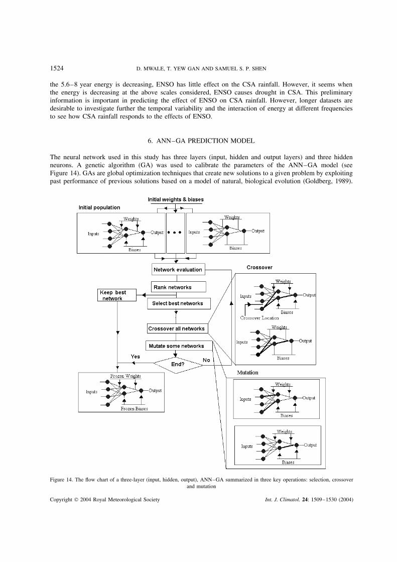
6. ANN–GA PREDICTION MODEL

The neural network used in this study has three layers (input, hidden and output layers) and three hiddenneurons. A genetic algorithm (GA) was used to calibrate the parameters of the ANN–GA model (seeFigure 14). GAs are global optimization techniques that create new solutions to a given problem by exploitingpast performance of previous solutions based on a model of natural, biological evolution (Goldberg, 1989).

Figure 14. The flow chart of a three-layer (input, hidden, output), ANN–GA summarized in three key operations: selection, crossoverand mutation



The solution space (or population) from which the individual solutions are drawn is represented in the form offinite lengths of strings called chromosomes. The adaptability of chromosomes is improved through a processof systematic modifications made up of crossover and mutation. For the ANN–GA model, the chromosomeswere made of weights and biases assigned to each node. The weights and biases have traditionally been foundusing the back-propagation algorithm (Rumelhart et al., 1986). In recent years, the back-propagation algorithmis less preferred compared with more efficient optimization algorithms, such as the conjugate gradient method,simulated annealing and GAs (Hsieh and Tang, 1998).

6.1. Population and initial evaluation

The ANN–GA creates an initial set of weights W1 and W2 and biases B1 and B2 (bold capital lettersindicate a population) for a large number of neural networks (e.g. 2300 ANNs). Since the starting point ofthe initial weights and biases of an ANN is not known, the weights are created in random fashion to ensurethat the initial population contains diverse information. In using an ANN–GA for prediction, each output ofthe neural network in the population is initially evaluated against a known predictand. The objective function(fitness) used was based on either the Pearson correlation or the root-mean-square error (RMSE). To evaluateeach neural network, the predictand y is obtained as a nonlinear translation of the weighted average of thepredictor data x, which has been normalized, i.e., x = (x − x)/σx :

hidunitpj =N∑

i=1

Wjixpi + Bjo (10)

where hidunitpj is the weighted input to the j th hidden unit, N is the total number of input nodes Wji (weightsfrom input unit i to j ), Bjo are the biases for hidden neuron j , and xpi is the ith input of pattern p (in ourcase SST PCs are used). The hidden layer undergoes a non-linear translation

f1(hidunitpj ) = 1

1 + e−hidunitpj

(11)

where f1(hidnunitpj ) is the j th neuron non-linear activation function, and

outpk =M∑

j=1

Wkjf1(hidunitpj ) + Bko (12)

ypk = f2(outpk) (13)

where M is the number of hidden units, Wkj represents the weight connecting the hidden node j to the outputk, Bko is the bias for output neuron k, ypk is the predicted output and f2 is a linear function.

6.2. Ranking the neural networks

All the neural networks are ranked according to the computed fitness: the best network at the top and theworst at the bottom. The best 85% of the ranked population is randomly selected to comprise offspring ofthe next generation. Selecting from the best 85% of the ranked population ensures that, on average, the newgeneration has comparatively better fitness than the original population. Selection thus shifts the search spacetowards improved solution spaces of the problem. In this study, the population is kept constant; hence, somemembers of the old population are selected more than once.

6.3. Crossover

Pairs of neural networks are selected, either randomly or in the same order in which they were selectedfrom the previous population, and their weights and biases are exchanged. This procedure is called crossover.



To effect exchange of weights and biases, a one-point crossover scheme was used. In one-point crossoverschemes, a single location is randomly chosen in the hidden layer and weights on either side of the locationare exchanged between the two neural networks (shown as dark lines in the inset to Figure 14). This procedureis repeated between all other pairs of neural networks in the population.

6.4. Mutation

Next, a small percentage (e.g. between 0.1 and 1% of the total population) is randomly selected and thena handful of weights and biases are randomly replaced (see dark lines in the inset to Figure 14). The processis called mutation, and is designed to restore good weights and biases eliminated during selection. Sincemutation is a purely random process, it is always kept to a minimum to prevent the search degenerating intoa random process. If mutation results in a better neural network, then that network will likely survive inthe next selection; but, if the mutation results in a more inferior individual, then that individual will likelyperish in the next selection. In this paper, 1% of the population of neural networks is randomly chosen anda proportion of their weights is randomly mutated. The neural networks are once again evaluated against thesame known predictand.

The above procedures are repeated through several epochs (or generations in GA terminology). At eachgeneration, the best network is kept until a better solution is found in successive generations. Convergenceis reached when at least 95% of the solutions have the same weights and biases. At the end of the run, theweights and biases of the best surviving network are kept to be used for making predictions with new inputdata.

7. PREDICTION OF CSA RAINFAL (1985–94)

7.1. Selection of SST predictor fields

The existence of 2–2.4 year periods found within the ENSO band (Section 5) and the strong seasonalassociations between the SST SAWP of the South Atlantic and Indian Oceans and the CSA rainfall WPCs(Section 3) suggests that: (1) CSA rainfall is predictable at interannual scales, and (2) prediction of CSArainfall based on the preceding AMJ SST of the two oceans is possible. From Figure 10(a) and (b), raw SSTpredictor data were extracted for the months of April, May and June from all regions of the oceans wherethe correlation between CSA WPC1 and the SAWP of the oceans exceeded 0.50. Since the autocorrelationof the SAWP and WPCs was high (average 0.9), from Equation (9), the effective lengths of the SAWP andthe WPCs decreased to about 3–4 years and the significant correlation between CSA WPCs and SST SAWPat the 95% level was above 0.997. The ocean areas covered by this level of correlation were small, andvery few data could be collected. Since the spatial correlation pattern between CSA WPC1 and CSA SAWP(Figure 3(a)) covering most of the region varied between 0.4 and 0.7, it was decided that actual SST databe collected from areas of the ocean where the correlation between CSA rainfall WPC1 and SST SAWPwas 0.5 or more. The actual data were standardized and averaged over the 3 months for each grid stationin the two oceans to give one AMJ data set. To speed up the computations, EOF analysis was applied tothe raw AMJ SST dataset and six PCs accounting for 87% of the SST data variance were used as inputdata to the ANN–GA prediction model. Standardized rainfall data from the 31 CSA grid stations wereused.

7.2. Evaluation of prediction skill

To assess the prediction skill of the ANN–GA for 11 years (i.e. between 1984 and 1994), the Pearsoncorrelation, the Hansen Kuipers (HK) skill score and RMSE were used. The Pearson correlation coefficient



ρ is computed as

ρ =

n∑k=1

(obsk − obs)(predk − pred)

[(n∑

k=1

(obsk − obs)2) (

n∑k=1

(predk − pred)2

)]1/2 (14)

where obsk and predk are the observed and predicted values, obs and pred their respective means, and n is thesample size. This ρ varies between +1 and −1, with the maximum and minimum values indicating perfectpositive and negative linear relationships respectively. To compute the HK skill score, the predicted andobserved rainfall data are grouped into categories, say ‘Dry’, ‘Near Normal’ and ‘Wet’. Tercile percentagesof below 33%, 33–66% and above 66% were used to define the categories in a square contingency table.

HK = H − Ec

T − Em(15)

where H is the total number of correct forecasts, T is the total number of forecasts obtainable with a perfectforecast model, Ec is the number of correct hits expected by chance and Em is the marginal number of correct(observation) hits expected by chance. For a K × K contingency table, the HK score may be expressed interms of probabilities as

HK =

K∑i=1

p(obsi , predi ) −K∑

i=1

p(obsi ) × p(predi )

1 −K∑

j=1

[p(obsj )]2

(16)

The HK score values range from −1 to +1. Perfect forecasts receive a score of one, random forecast receivea score of zero and forecasts inferior to random forecasts receive negative scores. The RMSE is computed as

RMSE =(

1

n

n∑k=1

(obsk − predk)2

) 12

(17)

An RMSE of zero indicates a perfect prediction.

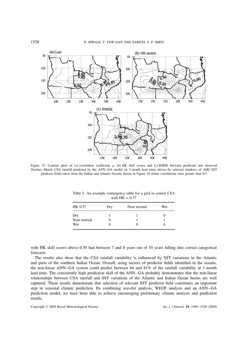
7.3. Skill of the predicted CSA rainfall

The spatial display of the correlation, HK skill scores and RMSEs between 10 years of predicted andobserved CSA rainfall is shown in Figure 15. Correlations of between 0.8 and 0.9, RMSEs of 0.4 and 0.9 andHK skill scores of between 0.4 and 0.8 were achieved for most of CSA. The skill decreased slightly towardsthe coastal areas, following the strength of CSA rainfall WPC1.

The high correlations show that the linear correlation between the predicted and observed rainfall wascaptured almost everywhere in CSA. The higher HK skill score also showed that most forecasts fell intheir correct categories. For example, Table I shows a categorical forecast for an area in central CSA.Out of 10 years, 8 years were correctly predicted by the ANN–GA. Table I also shows that most of theyears between 1985 and 1994 were wet (i.e. 6 years were wet, and 2 years had near-normal rainfall, and2 years were below-normal or dry) consistent with Figure 13(a), which shows that the period 1985–91 (i.e.7 years) was generally wet and 1992–94 experienced below-normal rainfall (or droughts). A look at Table Ishows that 2 years were wrongly predicted, one as wet and the other as near normal. Generally, areas



Figure 15. Contour plots of (a) correlation coefficient ρ, (b) HK skill scores and (c) RMSE between predicted and observedOctober–March CSA rainfall predicted by the ANN–GA model (at 3 month lead time) driven by selected windows of AMJ SST

predictor fields taken from the Indian and Atlantic Oceans shown in Figure 10 where correlations were greater than 0.5

Table I. An example contingency table for a grid in central CSAwith HK = 0.57

HK 0.57 Dry Near normal Wet

Dry 1 1 0Near normal 0 1 1Wet 0 0 6

with HK skill scores above 0.50 had between 7 and 8 years out of 10 years falling into correct categoricalforecasts.

The results also show that the CSA rainfall variability is influenced by SST variations in the Atlanticand parts of the southern Indian Ocean. Overall, using sectors of predictor fields identified in the oceans,the non-linear ANN–GA system could predict between 64 and 81% of the rainfall variability at 3 monthlead time. The consistently high prediction skill of the ANN–GA probably demonstrates that the non-linearrelationships between CSA rainfall and SST variations of the Atlantic and Indian Ocean basins are wellcaptured. These results demonstrate that selection of relevant SST predictor field constitutes an importantstep in seasonal climate prediction. By combining wavelet analysis, WEOF analysis and an ANN–GAprediction model, we have been able to achieve encouraging preliminary climate analysis and predictionresults.



8. SUMMARY AND CONCLUSIONS

Using wavelet analysis and WEOF analysis on SAWP and ISP, we identified the non-stationary SST fields ofthe South Atlantic and Indian Oceans that are associated with coherent regions of rainfall variability in CSA.The Benguela ocean current SSTs form the dominant spatial pattern of the South Atlantic Ocean. The spatialpatterns were found to migrate seasonally between Africa’s west coast and South America’s east coast. TheBrazil and Guinea ocean current SSTs form the second leading spatial patterns of variability of the AtlanticOcean. The northern Indian Ocean SST forms the leading spatial pattern, followed by the south Indian OceanSST. The Atlantic Ocean SST variability was found to have stronger associations with CSA rainfall variabilitythan the Indian Ocean SST.

The ISP WPCs show strong spatial and temporal variations at the 2–2.4 and 5.6–6.7 year cycles over CSA,whereas the time-domain WPCs accurately represent temporal variations of CSA rainfall. Further, it seemsthat CSA rainfall responded to ENSO only when simultaneous decreases of energy at 2–2.4 and 5.6–6.7 yearperiods occurred.

Using predictor fields identified from the Atlantic and Indian Oceans, the non-linear ANN–GA systemcould predict accurate CSA rainfall at 3 month lead times. At 3 month lead time, correlations between 0.8and 0.9, RMSEs between 0.4 and 0.9, and HK skill scores between 0.4 and 0.8 were obtained betweenobserved and predicted CSA rainfall.

ACKNOWLEDGEMENTS

This project was partly supported by NSERC of Canada. The first author was also supported by theCommonwealth scholarship of CIDA, Canada. The UK Meteorological Office provided both the SSTgrid data of the Indian and Atlantic Oceans (part of MOHSST6) and the rainfall data for CSA.The wavelet analysis was done using the software of Torrence and Compo (1998) downloaded fromhttp://www.paos/colorado.edu/research/wavelets.

REFERENCES

Allan RJ, Lindesay JA, Reason CJC. 1995. Multi-decadal variability in the climate system over the Indian Ocean region during theaustral summer. Journal of Climate 8: 1853–1873.

Bakshi B. 1998. Multiscale PCA with applications to multivariate statistical process monitoring. AIChE Journal 44: 1596–1610.Barnston AG, Thiao W, Kumar V. 1996. Long-lead forecasts of seasonal precipitation in Africa using CCA. Weather and Forecasting

11: 506–520.Basalirwa CPK. 1995. Delineation of Uganda into climatological rainfall zones using the method of principal component analysis.

International Journal of Climatology 15: 1161–1177.BBC 2002a. http://news.bbc.co.uk/2/hi/africa/2027079.stm [Accessed April 2004].BBC 2002b. http://news.bbc.co.uk/2/hi/africa/2504661.stm [Accessed April 2004].Castleman KR. 1996. Digital Image Processing. Prentice Hall: Englewood Cliffs, NJ.Fanta B, Zaake BT, Kachroo RK. 2001. A study of the variability of the river flow of the southern Africa region. Hydrological Sciences

4: 513–524.Goldberg DE. 1989. Genetic Algorithms in Search, Optimization and Machine Learning. Addison-Wesley: Reading, MA.Houghton RW, Tourre YM. 1992. Characteristics of low-frequency sea surface temperature fluctuations in the tropical Atlantic. Journal

of Climate 5: 765–771.Hsieh WW, Tang B. 1998. Applying neural network models to prediction and data analysis in meteorology and oceanography. Bulletin

of the American Meteorological Society 79: 1855–1868.Huang NE, Shen Z, Zheng Q, Yen N, Tung CC, Liu HH. 1998. The empirical mode decomposition and the Hilbert spectrum for

nonlinear and non-stationary time series analysis. Proceedings of the Royal Society of London 454: 903–995.Hulme M. 1994. Validation of large-scale precipitation fields in general circulation models. In Global Precipitations and Climate Change,

Desbois M, Desalmand F (eds). NATO ASI Series. Springer-Verlag: Berlin; 387–406.Hulme M, Conway DD, Joyce A. Mulenga H. 1996. A 1961–90 climatology of Africa south of the Equator and a comparison of

potential evapotranspiration estimates. South African Journal of Science 92: 334–343.Jury MR. 1996. Regional teleconnection pattern associated with summer rainfall over South Africa, Namibia and Zimbabwe.

International Journal of Climatology 16: 135–153.Jury MR, Engert S. 1999. Teleconnections modulating inter-annual climate variability over northern Namibia. International Journal of

Climatology 19: 1459–1475.Kutzbach JE. 1967. Empirical eigenvectors of sea-level pressure, surface temperature and precipitation complexes over North America.

Journal of Applied Meteorology 6: 791–802.



Landman WA, Mason SJ. 1999. Change in the association between Indian Ocean sea-surface temperatures and summer rainfall overSouth Africa and Namibia. International Journal of Climatology 19: 1477–1492.

Landman WE, Tennant WJ. 2000. Statistical downscaling of monthly forecasts. International Journal of Climatology 20: 1521–1532.Landman WE, Mason SJ, Tyson PD, Tennant WJ. 2001. Retroactive skill of multi-tiered forecasts of summer rainfall over southern

Africa. International Journal of Climatology 21: 1–19.Mason SJ. 1995. Sea-surface temperature–south African rainfall associations, 1910–1989. International Journal of Climatology 15:

119–135.Mason SJ. 1997. Review of recent developments in seasonal forecasting of rainfall. Water SA 23: 57–61.Mason SJ, Tyson PD. 2000. The occurrence and predictability of droughts over southern Africa. In Drought Volume 1: A Global

Assessment, Wilhite DA (ed.). Routledge: New York; 113–134.Mutai CC, Ward MN, Colman A. 1998. Towards the prediction of the East Africa short rains based on sea surface

temperature–atmosphere coupling. International Journal of Climatology 18: 975–997.Nicholson SE. 1986. The nature of rainfall variability in Africa south of the equator. Journal of Climatology 6: 515–530.Ntale HK, Gan TY, Mwale D. 2003. Prediction of East Africa seasonal rainfall using canonical correlation analysis. Journal of Climate

16(12): 2105–2112.Park J, Mann ME. 2000. Inter-annual temperature events and shifts in global temperature: a “multiwavelet” correlation approach. Earth

Interactions 4: 1–53.Reason CJC, Mulenga H. 1999. Relationships between South African rainfall and SST anomalies in the southwest Indian Ocean.

International Journal of Climatology 19: 1651–1673.Richard Y, Trzaska S, Roucou P, Rouault M. 2000. Modification of the southern African rainfall variability/ENSO relationship since

the late 1960s. Climate Dynamics 16: 883–895.Ropelewski CF, Halpert MS. 1987. Global and regional scale precipitation patterns associated with El Nino/southern oscillation. Monthly

Weather Review 115: 1601–1626.Rumelhart DE, Hinton GE, Williams RJ. 1986. Learning internal representations by error propagation. Parallel Distributed Processing,

Vol. 1, Rumelhart DE, McClelland JL, Group PR (eds). MIT Press: 318–362.Shen SPS, Lau WKM, Kim KY, Li G. 2001. A canonical ensemble correlation prediction model for seasonal precipitation anomaly ,

Technical memorandum NASA/TM-2001-209989, Greenbelt, MD.Smith LC, Turcotte DL, Isacks BL. 1998. Streamflow characterization and feature detection using a discrete wavelet transform.

Hydrological Processes 12: 233–249.Torrence C, Compo GP. 1998. A practical guide to wavelets analysis. Bulletin of the American Meteorological Society 1: 61–78.United Nations Development Program/Food and Agriculture Organization of the United Nations report. Multipurpose Survey of the

Kafue River Basin, Zambia Final Report (FAO/SF:35/ZAM), Volume III, Climatology and Hydrology.Wang B, Wang Y. 1996. Temporal structure of the southern oscillation as revealed by waveform and wavelet analysis. Journal of

Climate 9: 1586–1598.Venegas SA, Mysak LA, Straub DN. 1997. Atmosphere–ocean coupled variability in the South Atlantic. Journal of Climate 10:

2904–2920.Webster PJ, Clark C, Cherikova G, Fasullo J, Han W, Loschnigg J, Sahami K. 2002. The monsoon as a self-regulating coupled

ocean–atmosphere system. In Meteorology at the Millennium, Pearce RP (ed.). International Geophysics Series, vol. 83. AcademicPress: San Diego; 198–219.

Wilks DS. 1995. Statistical Methods in the Atmospheric Sciences. Academic Press: San Diego.


Documents

A new analysis of variability and predictability of