A N e w Ge n e r al M e th od to Ge n e r ate R an d om M ... · In Section 2 we recall a lis t o f desira ble fea tures for g ood test se ts. ... the advanced version of ou r metho

Journal of Artificial Intelligence Research 18 (2003) 351–389 Submitted 10/02; published 5/03

A New General Method to Generate Random Modal Formulae for

Testing Decision Procedures

Peter F. Patel-Schneider [email protected]

Bell Labs Research, 600 Mountain Ave., Murray Hill, NJ 07974, USA

Roberto Sebastiani [email protected]

Dip. di Informatica e Telecomunicazioni, Universita di Trento, via Sommarive 14, I-38050, Trento, Italy

Abstract

The recent emergence of heavily-optimized modal decision procedures has highlighted the key

role of empirical testing in this domain. Unfortunately, the introduction of extensive empirical tests

for modal logics is recent, and so far none of the proposed test generators is very satisfactory. To

cope with this fact, we present a new random generation method that provides benefits over pre-

vious methods for generating empirical tests. It fixes and much generalizes one of the best-known

methods, the random CNF¾Ñtest, allowing for generating a much wider variety of problems, cov-

ering in principle the whole input space. Our newmethod produces much more suitable test sets for

the current generation of modal decision procedures. We analyze the features of the new method

by means of an extensive collection of empirical tests.

1. Motivation and goals

Heavily-optimized systems for determining satisfiability of formulae in propositional modal logics

are now available. These systems, including DLP (Patel-Schneider, 1998), FaCT (Horrocks, 1998),

*SAT (Giunchiglia, Giunchiglia, & Tacchella, 2002), MSPASS (Hustadt, Schmidt, &Weidenbach,

1999), and RACER (Haarslev & Moller, 2001), have more optimizations and are much faster than

the previous generation of modal decision procedures, such as leanK (Beckert & Gore, 1997), Log-

ics Workbench (Heuerding, Jager, Schwendimann, & Seyfreid, 1995), ¾KE (Pitt & Cunningham,

1996) and KSAT (Giunchiglia & Sebastiani, 2000).1

As with most theorem proving problems, neither computational complexity nor asymptotic al-

gorithmic complexity is very useful in determining the effectiveness of optimizations, so that their

effectiveness has to be determined by empirical testing (Horrocks, Patel-Schneider, & Sebastiani,

2000). Empirical testing directly gives resource consumption in terms of compute time and memory

use; it factors in all the pieces of the system, not just the basic algorithm itself. Empirical testing

can be used not only to compare different systems, but also to tune a system with parameters that

can be used to modify its performance; moreover, it can be used to show what sort of inputs the

system handles well, and what sort of inputs the system handles poorly.

Unfortunately, the introduction of extensive empirical tests for modal logics is recent, and so

far none of the proposed test methodologies are very satisfactory. Some methods contain many

formulae that are too easy for current heavily-optimized procedures. Some contain high rates of

trivial or insignificant tests. Some generate problems that are too artificial and/or are not a significant

1. For a more complete list see Renate Schmidt’s Web page listing theorem provers for modal logics at

http://www.cs.man.ac.uk/˜schmidt/tools/.

c2003 AI Access Foundation and Morgan Kaufmann Publishers. All rights reserved.

PATEL-SCHNEIDER AND SEBASTIANI

sample of the input space. Finally, some methods generate formulae that are too big to be parsed

and/or handled.

For the reasons described above, we presented (Horrocks et al., 2000) an analytical survey of

the state-of-the art of empirical testing for modal decision procedures. Here instead we present a

new random generation method that provides benefits over previous methods for generating empir-

ical tests, built on some preliminary work (Horrocks et al., 2000). Our new method fixes and much

generalizes the 3CNF¾Ñ methodology for randomly generating clausal formulae in modal logics

(Giunchiglia & Sebastiani, 1996; Hustadt & Schmidt, 1999; Giunchiglia, Giunchiglia, Sebastiani,

& Tacchella, 2000) used in many previous empirical tests of modal decision procedures. It elimi-

nates or drastically reduces the influence of a major flaw of the previous method,2 and allows for

generating a much wider variety of problems.

In Section 2 we recall a list of desirable features for good test sets. In Section 3 we briefly

survey the state-of-the-art test methods. In Sections 4 and 5 we present and discuss the basic and

the advanced versions of our new test method respectively, and evaluate their features by presenting

a large amount of empirical results. In Section 6 we provide a theoretical result showing how

the advanced version of our method, in principle, can cover the whole input space. In Section 7

we discuss the features of our new method, and compare it wrt. the state-of-the-art methods. In

Section 8 we conclude and indicate possible future research directions.

A 5-page system description of our random generator has been presented at IJCAR’2001 (Patel-

Schneider & Sebastiani, 2001).

2. Desirable features for good test sets

The benefits of empirical testing depend on the characteristics of the inputs provided for the testing,

as empirical testing only provides data on these particular inputs. If the inputs are not typical or

suitable, then the results of the empirical testing will not be useful. This means that the inputs

for empirical testing must be carefully chosen. With Horrocks (Horrocks et al., 2000) we have

previously proposed and motivated the following key criteria for creating good test sets.

Representativeness: The ideal test set should represent a significant sample of the whole input

space. A good empirical test set should at least cover a large area of inputs.

Difficulty: A good empirical test set should provide a sufficient level of difficulty for the system(s)

being tested. (Some problems should be too hard even for state-of-the-art systems, so as to

be a good benchmark for forthcoming systems.)

Termination: To be of practical use, the tests should terminate and provide information within a

reasonable amount of time. If the inputs are too hard, then the system may not be able to

provide answers within the established time. This inability of the system is of interest, but

can make system comparison impossible or insignificant.

Scalability: The difficulty of problems should scale up, as comparing absolute performances may

be less significant than comparing how performances scale up with problems of increasing

difficulty.

2. That is, a significant amount of inadvertently trivial problems are generated unless the parameter p is set to 0 (Hor-

rocks et al., 2000). See Section 4.1 for a full discussion of this point.

352

A NEW GENERAL METHOD TO GENERATE RANDOM MODAL FORMULAE

Valid vs. not-valid balance: In a good test set, valid and not-valid problems should be more or

less equal both in number and in difficulty. Moreover, the maximum uncertainty regarding the

solution of the problems is desirable.

Reproducibility: A good test set should allow for easily reproducing the results.

The following criteria derive from or are significant sub-cases of the main criteria above.

Parameterization: Parameterized inputs with sufficient parameters and degrees of freedom allow

the inputs to range over a large portion of the input space.

Control: In particular, it is very useful to have parameters that control monotonically the key fea-

tures of the input test set, like the average difficulty and the “valid vs. non-valid” rate.

Modal vs. propositional balance: Reasoning in modal logics involves alternating between two or-

thogonal search efforts: pure modal reasoning and pure propositional reasoning. A good test

set should be challenging from both viewpoints.

Data organization: The data should be summarizable —so as to make a comparison possible with

a limited effort— and plottable —so as to enable the qualitative behavior of the system(s) to

be highlighted.

Finally, particular care must be taken to avoid the following problems.

Redundancy: Empirical test sets must be carefully chosen so as not to include inadvertent redun-

dancy. They should also be chosen so as not to include small sub-inputs that dictate the result

of the entire input.

Triviality: A good test set should be flawless, that is, it should not contain significant subsets of

inadvertent trivial problems.

Artificiality: A good empirical test set should correspond closely to inputs from applications.

Over-size: The single problems should not be too big w.r.t. their difficulty, so that the resources

required for parsing and data managing do not seriously influence total performance.

These criteria, which are described and motivated in detail by Horrocks et al. (2000), have been

proposed after a five-year debate on empirical testing in modal logics (Giunchiglia & Sebastiani,

1996; Heuerding & Schwendimann, 1996; Hustadt & Schmidt, 1999; Giunchiglia et al., 2000;

Horrocks & Patel-Schneider, 2002). (Notice that some of these criteria are identical or similar to

those suggested by Heuerding and Schwendimann (1996).)

The above criteria are general, and in some cases they require some interpretation. First, some

of them have to be implicitly interpreted as “unless the user deliberately wants the contrary for some

reason”. For instance, it might be the case that one wants to deliberately generate easy problems,

e.g., to be sure that the tested procedure does not take too much time to solve them, or redundant

problems, e.g., to test the effectiveness of some redundancy elimination technique, or satisfiable

problems only, e.g., to test incomplete procedures. To this extent, the key issue here is having a

reasonable form of control over these features, so that one can address not only general-purpose

criteria, but also specific desiderata.

353


Second, in some cases, there may be a tradeoff between two distinct criteria, so that it may

be necessary to choose only one of them, or to make a compromise. One example is given by

redundancy and artificiality: in some real-world problems large parts of the knowledge base are

irrelevant for the query, whose result is determined by a small subpart of the input; in this sense

eliminating such “redundancies” may make problems more “artificial”.

Particular attention must be paid to the problem of triviality, as it has claimed victims in many

areas of AI. In fact, flaws (i.e., inadvertent trivial problems) have been detected in random generators

for SAT (Mitchell, Selman, & Levesque, 1992), CSP (Achlioptas, Kirousis, Kranakis, Krizanc, Mol-

loy, & Stamatiou, 1997; Gent, MacIntyre, Prosser, Smith, & Walsh, 2001), modal reasoning (Hus-

tadt & Schmidt, 1999) and QBF (Gent & Walsh, 1999). Thus, the notion of “trivial” (and thus

“flawed”) deserves more comment.

In the work by Achlioptas et al. (1997) flawed problems are those solvable in linear time by

standard CSP procedures, due to the undesired presence of implicit unary constraints causing some

variable’s value to be inadmissible. A similar notion holds for SAT (Mitchell et al., 1992) and QBF

(Gent & Walsh, 1999). In the literature of modal reasoning, instead, the typical flawed problems

are those whose (un)satisfiability can be verified directly at propositional level, that is, without

investigating any modal successors; this kind of problems are typically solved in negligible time

w.r.t. other problems of similar size and depth (Hustadt & Schmidt, 1999; Giunchiglia et al., 2000;

Horrocks et al., 2000).3 Thus, with a little abuse of notation and when not otherwise specified, in

this paper we will call trivially (un)satisfiable the problems of this kind.4

3. An overview of the state-of-the-art

Previous empirical tests have mostly been generated by three methods: hand-generated formulae

(Heuerding & Schwendimann, 1996), randomly-generated clausal modal formulae (Giunchiglia &

Sebastiani, 1996; Hustadt & Schmidt, 1999; Giunchiglia et al., 2000), and randomly-generated

quantified boolean formulae that are then translated into modal formulae (Massacci, 1999).

We have already presented a detailed analysis of these three methods (Horrocks et al., 2000).

Here we present only a quick overview of the latter two methods, as we will refer to them in follow-

ing sections.5

3.1 The 3CNF¾Ñ Random Tests

In the 3CNF¾Ñ test methodology (Giunchiglia & Sebastiani, 1996; Hustadt & Schmidt, 1999;

Giunchiglia et al., 2000), the performance of a system is evaluated on sets of randomly gener-

ated 3CNF¾Ñ formulae. A CNF¾Ñ formula is a conjunction of CNF¾Ñ clauses, where each clause

is a disjunction of either propositional or modal literals. A literal is either an atom or its negation.

Modal atoms are formulae of the form ¾iC , where C is a CNF¾Ñ clause. A 3CNF¾Ñ formula is a

CNF¾Ñ formula where all clauses have exactly 3 literals.

3. Of course here by “modal” we implicitly assume the modal depth be strictly greater than zero, that is, we do not

consider purely propositional formulas.

4. Notice that we do not use the more suitable expression “propositionally (un)satisfiable” because the latter has been

used with a different meaning in the literature of modal reasoning (see, e.g., (Giunchiglia & Sebastiani, 1996, 2000)).

5. The first method (Heuerding & Schwendimann, 1996) is obsolete, as the formulae generated are too easy for current

state-of-the-art deciders (Horrocks et al., 2000).

354


3.1.1 THE RANDOM GENERATOR

A 3CNF¾Ñ formula is randomly generated according to five parameters: the (maximum) modal

depth d; the number of clauses in the top-level conjunction Ä; the number of propositional variablesÆ ; the number of distinct box symbols Ñ; and the probability Ô of an atom occurring in a clause at

depth < d being purely propositional.

The random 3CNF¾Ñ generator, in its final version (Giunchiglia et al., 2000), works as follows:

¯ a 3CNF¾Ñ formula of depth d is produced by randomly generating Ä 3CNF¾Ñ clauses of

depth d, and forming their conjunction;

¯ a 3CNF¾Ñ clause of depth d is produced by randomly generating three distinct, under com-mutativity of disjunction, 3CNF¾Ñ atoms of depth d, negating each of them with probability

0.5, and forming their disjunction;

¯ a propositional atom is produced by picking randomly an element of fA½; : : : ; AÆ g with

uniform probability;

¯ a 3CNF¾Ñ atom of depth d > ¼ is produced by generating with probability Ô a randompropositional atom, and with probability ½ Ô a 3CNF¾Ñ atom ¾ÖC , where ¾Ö is picked

randomly in f¾½; : : : ;¾Ñg and C is a randomly generated 3CNF¾Ñ clause of depth d ½.

Recently Horrocks and Patel-Schneider (2002) have proposed a variant of the 3CNF¾Ñ random

generator of Giunchiglia et al. (2000). They added four extra parameters: ÒÔ and ÒÑ, representing

respectively the probability that a propositional and modal atom is negated, and cÑiÒ and cÑaÜ,

representing respectively the minimum and maximum number of modal literals in a clause, with

equal probability for each number in the range. For their experiments, they always set ÒÔ = ¼:5and cÑiÒ = cÑaÜ = ¿. To this extent, 3CNF¾Ñ formulas can be generated as in the generator of

Giunchiglia et al. (2000) by setting ÒÔ = ÒÑ = ¼:5 and cÑiÒ = cÑaÜ = ¿.

3.1.2 TEST METHOD & DATA ANALYSIS

The 3CNF¾Ñ test method works as follows. A typical problem set is characterized by a fixed

Æ , Ñ, d and Ô: Ä is varied in such a way as to empirically cover the “100% satisfiable—100%

unsatisfiable” transition. Then, for each tuple of the parameters’ values (data point from now on)

in a problem set, a certain number of 3CNF¾Ñ formulae are randomly generated, and the resulting

formulae are given in input to the procedure under test, with a maximum time bound. Satisfiability

rates, median/percentile values of the CPU times, and median/percentile values of other parameters,

e.g., number of steps, memory, etc., are plotted against the number of clauses Ä or the ratio of

clauses to propositional variables Ä=Æ .

3.2 The Random QBF Tests

In QBF-based benchmarks (such as part of the TANCS’99 benchmarks (Massacci, 1999)), sys-

tem performances are evaluated on sets of random quantified boolean formulae, which are gener-

ated according to the method described by Cadoli, Giovanardi, and Schaerf (1998) and Gent and

Walsh (1999) and then converted into modal logic by using a variant of the conversion by Halpern

and Moses (1992).

355


3.2.1 THE RANDOM GENERATOR

Random QBF formulae are generated with alternation depth D and at most Î variables at each

alternation. The matrix is a random propositional CNF formula with C clauses of length Ã , with

some constraints on the number of universally and existentially quantified variables within each

clause. (This avoids the problem of generating flawed random QBF formulae highlighted by Gent

and Walsh (1999).) For instance, a random QBF formula with D = ¿, Î = ¾ looks like:

8Ú¿¾Ú¿½:9Ú¾¾Ú¾½:8Ú½¾Ú½½:9Ú¼¾Ú¼½: [Ú¿¾; :::; Ú¼½]: (1)

Here is a random CNF formula with parameters C , Î and D. We will denote with Í and Ethe total number of universally and existentially quantified variables respectively. Clearly, both Íand E are Ç´D ¡ Î µ. Moreover, ³ is the modal formula resulting from Halpern and Moses’ Ã

conversion, so both the depth d and the number of propositional variables Æ of ³ are also Ç´D ¡Î µ.

3.2.2 TEST METHOD & DATA ANALYSIS

The test method, as it was used in the TANCS competition(s) (Massacci, 1999), works as follows.

The tests are performed on single data points. For each data point, a certain number of QBF

formulae are randomly generated, converted into modal logics and the resulting formulae are given

as input to the procedure being tested, with a maximum time bound. The number of tests which

have been solved within the time-limit and the geometrical mean time for successful solutions are

then reported. Data are rescaled to abstract away machine and run-dependent characteristics. This

results typically in a collection of tables presenting a data pair for each system under test, one data

point per row.

4. A new CNF¾Ñ generation method: basic version

From our previous analysis (Horrocks et al., 2000) we have that none of the current methods are

completely satisfactory. To cope with this fact, we propose here what we believe is a much more sat-

isfactory method for randomly generating modal formulae. The new method can be seen as an im-

proved and much more general version of the random 3CNF¾Ñ generation method by Giunchiglia

et al. (2000).

We present our new method by introducing incrementally its new features in two main steps. In

this section we introduce a basic version of the method, wherein

¯ we provide a new interpretation for the parameter Ô (Section 4.1) that allows for varying Ôwithout causing the flaws described in Horrocks et al. (2000); and

¯ we extend the interpretation for the parameter C (Section 4.3), providing a more fine-grained

way for tuning the difficulty of the generated formulae.

In Section 5, we present the full, advanced version of the method, wherein

¯ we further extend the parameters Ô and C , allowing for shaping explicitly the probability

distribution of the propositional/modal rate and the clause length respectively (Section 5.1);

and

¯ we allow Ô and C vary with the nesting depth of the subformulae (Section 5.2), allowing for

different distributions at different depths.

356


To investigate the properties of our CNF¾Ñ generator we also present a series of experiments with

appropriate settings either to mimic previous generation methodologies or to produce improved or

new kinds of tests.

In all tests we have adopted the testing criteria of the 3CNF¾Ñ method. For each test set, we

fixed all parameters except Ä, which was varied to span at least the satisfiability transition area.(Because of the “Valid vs. non-valid balance” feature of Section 2, we consider the transition area

to be the interesting portion of the test set.) For almost all test sets we varied Ä from Æ to ½¾¼Æ ,

½5¼Æ , or ¾¼¼Æ , resulting in integral values for Ä=Æ ranging from ½ to ½¾¼, ½5¼, or ¾¼¼. For eachvalue of Ä we generated 100 formulae, a sufficient number to produce reasonably reliable data. A

time limit of 1000 seconds was imposed on each attempt to determine the satisfiability status of a

formula. As it is common practice, we set the number of boxes Ñ to ½ throughout our testing. Thissetting for Ñ produces the hardest formulae (Giunchiglia & Sebastiani, 1996; Hustadt & Schmidt,

1999; Giunchiglia et al., 2000). We performed several test sets with similar parameters, often, but

not always, varying only Æ .

We tested our formulae against two systems, DLP version 4.1 (Patel-Schneider, 1998) and *SAT

version 1.3 (Tacchella, 1999), two of the fastest modal decision procedures. They are available re-

spectively under http://www.bell-labs.com/usr/pfps/dlp and http://www.mrg.dist.unige.it/˜tac.

All the code used to generate the tests is available under http://www.bell-labs.com/usr/pfps/dlp.

We plotted the results of our test groups (test sets with similar parameters) on six or four plots.

Two plots were devoted to the performance of DLP, one showing the median and one showing the

90th percentile time taken to solve the formulae at each value of Ä, plotted against Ä=Æ . For those

test groups were we ran *SAT we also plotted the median and 90th percentile for *SAT.

We also plotted the fraction of the formulae that are determined to be satisfiable or unsatisfiable

by DLP within the time limit.6 To save space, satisfiability and unsatisfiability fractions are plotted

together on a single plot. Satisfiability fractions are higher on the left side of the plot while unsat-

isfiability fractions are higher on the right. This multiple plotting does obscure some of the details,

but the only information that we are interested in here is the general behavior of the fractions, which

is not obscured. In fact, the multiple plotting serves to highlight the crossover regions, where the

satisfiability and unsatisfiability fractions are roughly equal.

Finally, we plotted the fraction of the formulae where DLP finds a model or determines that

the formula is unsatisfiable without investigating any modal successors. We call these fractions

the trivial satisfiability and trivial unsatisfiability fractions. These last fractions are an estimate

of the number of formulae that are satisfiable in a Kripke structure with no successors —like, e.g.,

Á½ _ ¾½A¾µ— and that have no propositional valuations —like, e.g., ´¾½A½ ^ :¾½A½µ— respec-

tively. For various reasons, discussed below, they are better indicators of triviality than the more

formal measures used in previous papers. Again, trivial satisfiability and unsatisfiability fractions

are plotted together on a single plot.

To reduce clutter on the plots, we used a line to show the results for each value of Ä we tested.

To distinguish between the various lines on a plot, we plotted every five or 10 data points with a

symbol, identified in the legend of the plot.

Running the tests presented in this paper required some months of CPU time. Because of this,

we ran our tests on a variety of machines. These machines range in speed from a 296MHz SPARC

6. Notice that the two curves are symmetric with respect to 0.5 if and only if no test exceeds the time limit. E.g., if at

some point 40% of the tests are determined to be satisfiable by DLP, 10% are determined to be unsatisfiable and 50%

are not solved within the time limit, then the two curves are not symmetric at that point, as ¼:4¼ 6= ½ ¼:½¼.

357


Ultra 2 to a 400MHz SPARC Ultra 4 and had between 256MB and 512MB of main memory. No

machines were completely dedicated to our tests, but they were otherwise lightly loaded. Each test

set was run on machines with the same speed and memory. Direct comparison between different

groups of tests thus has to take into account the differences between the various test machines.

4.1 Reinterpreting the parameter Ô

One problem with the previous methods for generating CNF¾Ñ formulae is that the generated for-

mulae can contain pieces that make the entire formula easy to solve. This mostly results from the

presence of strictly-propositional top-level clauses. With the small number of propositional vari-

ables in most tests (required to produce reasonable difficulty levels for current systems), only a

few strictly-propositional top-level clauses are needed to cover all the combinations of the proposi-

tional literals and make the entire formula unsatisfiable. Previous attempts to eliminate this “trivial

unsatisfiability” have concentrated on eliminating top-level propositional literals by setting Ô = ¼(Hustadt & Schmidt, 1999; Giunchiglia et al., 2000). (Unfortunately this choice forces d ½,as for d > ½ such formulae are too hard for all state-of-the-art systems.) When each atom in a

clause is generated independently from the other atoms of the clause an approach that modifies the

probability of propositional atoms is necessary to eliminate these problematic clauses.

The first new idea of our approach, suggested previously (Horrocks et al., 2000), works as

follows. Instead of forbidding strictly-propositional clauses except at the maximum modal depth, d,by setting Ô = ¼, we instead require that the ratio between propositional atoms in a clause and theclause size be as close as possible to the propositional probability Ô for clauses not at the maximummodal depth d. 7

For clauses of size C , if Ô is k=C for some integral k, this results in all clauses not at modaldepth d having k propositional atoms and C k modal atoms. For other values of Ô, we alloweither bÔCc or dÔCe propositional atoms in each clause not at modal depth d, with probabilitydÔCe ÔC and ÔC bÔCc, respectively.8 For instance, if Ô = ¼:6 and C = ¿, then each clausecontains 1 propositional and 1 modal literal, and the third is propositional with probability 0.8, as

¿ ¡ ¼:6 b¿ ¡ ¼:6c = ½:8 ½ = ¼:8. If Ô Ć ½µ=C , this eliminates the possibility of strictlypropositional clauses, which are the main cause of trivial unsatisfiability, except at modal depth d.

4.1.1 MODAL DEPTH ½

Our first experiments were a direct comparison to previous tests. We generated CNF¾Ñ formulae

with C = ¿, Ñ = ½, d = ½, and Ô = ¼:5, a setting that has been used in the past, and one thatexhibits some problematic behavior. We used both our new method and the old 3CNF¾Ñ generation

method by Giunchiglia et al. (2000) briefly described in Section 3.1 (the “old method” from now

on). We also generated CNF¾Ñ formulae with C = ¿, Ñ = ½, d = ½, and Ô = ¼, the standardmethod for eliminating trivially unsatisfiable formulae. (At Ô = ¼ our new method is the same as

the old 3CNF¾Ñ generation method.) The results of the tests are given in Figures 1, 2, and 3.

7. Other approaches to eliminating propositional unsatisfiability are possible. For example, it would be possible to

simply remove any strictly-propositional clauses after generation. However, this technique would alter the meaning

of the parameter Ô, that is, the actual probability for a literal to be propositional would become strictly smaller thanÔ, and it will be out of the control of the user.

8. Remember that bÜc =def ÑaÜfÒ ¾ ÆjÒ Xg and dÜe =def ÑiÒfÒ ¾ ÆjÒ Xg.

358


Satisfiability and Unsatisfiability Fractions Trivial Satisfiability and Unsatisfiability Fractions

0

0.2

0.4

0.6

0.8

1

20 40 60 80 100 120

L/N

N=3N=4N=5N=6N=7N=8N=9

0

0.2

0.4

0.6

0.8

1

20 40 60 80 100 120

L/N

N=3N=4N=5N=6N=7N=8N=9

DLP median times DLP 90th percentile times

0.01

0.1

1

10

100

1000

20 40 60 80 100 120

L/N

N=3N=4N=5N=6N=7N=8N=9

0.01

0.1

1

10

100

1000

20 40 60 80 100 120

L/N

N=3N=4N=5N=6N=7N=8N=9

*SAT median times *SAT 90th percentile times

0.01

0.1

1

10

100

1000

20 40 60 80 100 120

L/N

N=3N=4N=5N=6N=7N=8N=9

0.01

0.1

1

10

100

1000

20 40 60 80 100 120

L/N

N=3N=4N=5N=6N=7N=8N=9

Figure 1: Results for C = ¿,Ñ = ½, d = ½, and Ô = ¼:5 (old method)

One aspect of this set of tests is that all three collections have many trivially unsatisfiable formu-

lae out of the satisfiability transition area, even the collection with no top-level propositional atoms.

The trivial unsatisfiability occurs in the collection with no top-level propositional atoms because

there are only a few top-level modal atoms (e.g., 8 for Æ = ¿) and both DLP and *SAT detect

clashes between complementary modal literals without investigating any modal successors.

The presence of this large number of trivially unsatisfiable formulae is not actually a serious

problem with these tests. The trivial unsatisfiability only shows up after the formulae are almost

all unsatisfiable already and easy to solve. The only exception is for Æ = ¿, which is trivial tosolve anyway. However, our new generation method considerably reduces the number of trivially

unsatisfiable formulae and almost entirely removes them from the satisfiable/unsatisfiable transition

359



0

0.2

0.4

0.6

0.8

1

20 40 60 80 100 120

L/N

N=3N=4N=5N=6N=7N=8N=9

0

0.2

0.4

0.6

0.8

1

20 40 60 80 100 120

L/N

N=3N=4N=5N=6N=7N=8N=9


0.01

0.1

1

10

100

1000

20 40 60 80 100 120

L/N

N=3N=4N=5N=6N=7N=8N=9

0.01

0.1

1

10

100

1000

20 40 60 80 100 120

L/N

N=3N=4N=5N=6N=7N=8N=9


0.01

0.1

1

10

100

1000

20 40 60 80 100 120

L/N

N=3N=4N=5N=6N=7N=8N=9

0.01

0.1

1

10

100

1000

20 40 60 80 100 120

L/N

N=3N=4N=5N=6N=7N=8N=9

Figure 2: Results for C = ¿,Ñ = ½, d = ½, and Ô = ¼:5 (our new method)

area. There are some trivially satisfiable formulae in this set of tests, but only a few, and only for

the smallest clause sizes. Their presence does not affect the difficulty of the generated formulae.

The two methods with Ô = ¼:5 are relatively close in maximum difficulty, with our new method

generating somewhat harder formulae. However, our method produces difficult formulae, for both

DLP and *SAT, over a much broader range of Ä=Æ than does the original method.

Changing to Ô = ¼ results in formulae that are orders of magnitude harder. This is not good,previous arguments to the contrary notwithstanding, as we would like to have a significant number

of reasonable test sets to work with, and Ô = ¼ allows only consideration of a very few values for

Æ before the formulae are totally impossible to solve with current systems, resulting in very few

reasonable test sets.

360



0

0.2

0.4

0.6

0.8

1

20 40 60 80 100 120

L/N

N=3N=4N=5N=6

0

0.2

0.4

0.6

0.8

1

20 40 60 80 100 120

L/N

N=3N=4N=5N=6


0.01

0.1

1

10

100

1000

20 40 60 80 100 120

L/N

N=3N=4N=5N=6

0.01

0.1

1

10

100

1000

20 40 60 80 100 120

L/N

N=3N=4N=5N=6


0.01

0.1

1

10

100

1000

20 40 60 80 100 120

L/N

N=3N=4N=5N=6

0.01

0.1

1

10

100

1000

20 40 60 80 100 120

L/N

N=3N=4N=5N=6

Figure 3: Results for C = ¿,Ñ = ½, d = ½, and Ô = ¼ (either method).

So, at a maximum modal depth of d = ½ our method results in formulae that are of similardifficulty to the previously-generated formulae and still have trivially unsatisfiable formulae, but

ones that do not seriously affect the difficulty of the test sets.

4.1.2 MODAL DEPTH ¾

Restricting attention to a maximum modal depth of d = ½ is not very useful. Formulae with max-imum modal depth of ½ are not representative of modal formulae in general, particularly as theyhave no nested modal operators. Sticking to a maximum modal depth of ½ seriously limits the

significance of the generated tests.

361


We would thus like to be able to perform interesting experiments with larger maximum modal

depths. So we performed a set of experiments with a maximum modal depth of d = ¾. We startedwith a set of tests that corresponds to previously-performed experiments.

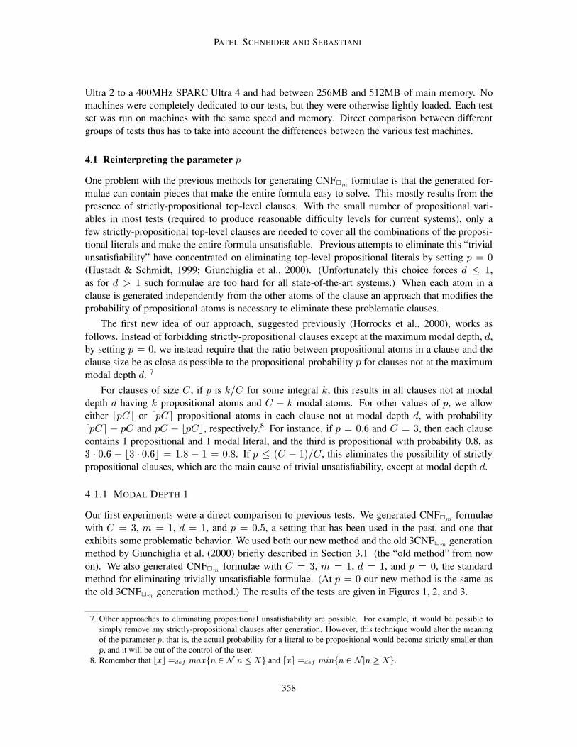
At depth d = ¾, in the old method for Ô = ¼:5 the time curves are dominated by a “half-dome”shape, whose steep side shows up where the number of trivially unsatisfiable formulae becomes

large before the formulae become otherwise easy to solve, as shown in Figure 4. In fact, nearly all

the unsatisfiable formulae here are trivially unsatisfiable.

This is an extremely serious flaw, as the difficulty of the test set is being drastically affected

by these trivially unsatisfiable formulae. Changing to Ô = ¼ is not a viable solution because at

depth d = ¾ such formulae are much too difficult to solve, as shown in Figure 5, where the medianpercentile exceeds the timeout before any formulae can be determined to be unsatisfiable, even for

3 propositional variables.

With our new method, as shown in Figure 6, the formulae are much more difficult to solve than

the old method, because there is no abrupt drop-off from propositional unsatisfiability, but they are

much easier to solve than those generated with Ô = ¼. Further, trivially unsatisfiable formulae donot appear at all in the interesting portion of the test sets.

Nevertheless this choice of parameters (d = ¾, Ô = ¼:5) is not entirely suitable. The formulaeare becoming too hard much too early. In particular, there are no unsatisfiable formulae that can

be solved for Æ > ¿, and thus the unsatisfiability plots cannot be distinguished from the x axis

(recall Footnote 6). However, our new method does provide some advantages already, providing an

interesting new set of tests, albeit one of limited size.

4.2 Increasing Ô

We would like to be able to produce better test sets for depth d = ¾ and greater. One way of

doing this is to increase the propositional probability Ô from ¼:5 to something like ¼:6, increasingthe number of propositional atoms and thus decreasing the difficulty of the generated formulae.

This would be very problematic with previous generation methods as it would result in the trivially

unsatisfiable formulae determining the results for even smaller numbers of clauses Ä, but with ourmethod here it is not much of a problem.

To investigate the increasing of the the propositional probability, we ran a collection of tests with

maximum modal depth d = ¾ and propositional probability Ô = ¼:6 with both the old method andour new method. The results of these tests are given in Figures 7 and 8. As before, the asymmetries

between the satisfiability and unsatisfiability curves in Figure 8 for Æ = 5; 6 are due to the fact thatmany tests are not solved by DLP within the time limit (c.f., Footnote 6).

As expected, the old method produces large numbers of trivially unsatisfiable formulae. These

trivially unsatisfiable formulae show up much earlier than with Ô = ¼:5, making the tests consider-ably easier, especially for *SAT.

Our new method produces hard formulae, but ones that are quite a bit easier than for Ô = ¼:5.In particular, DLP solved all instances within the time limit for Æ = 4. Trivially unsatisfiable

formulae do show up, but only well after the formulae are already unsatisfiable, and they do not

significantly affect the difficulty of the tests.

So our method allows the creation of more-interesting tests at modal depths greater than ½,simply by adjusting Ô to a value where the level of difficulty is appropriate. Trivial unsatisfiabilityis not a problem, whereas in the old method it was the most important feature of the test.

362



0

0.2

0.4

0.6

0.8

1

20 40 60 80 100 120 140 160 180 200

L/N

N=3N=4N=5N=6

0

0.2

0.4

0.6

0.8

1

20 40 60 80 100 120 140 160 180 200

L/N

N=3N=4N=5N=6


0.01

0.1

1

10

100

1000

20 40 60 80 100 120 140 160 180 200

L/N

N=3N=4N=5N=6

0.01

0.1

1

10

100

1000

20 40 60 80 100 120 140 160 180 200

L/N

N=3N=4N=5N=6


0.01

0.1

1

10

100

1000

20 40 60 80 100 120 140 160 180 200

L/N

N=3N=4N=5N=6

0.01

0.1

1

10

100

1000

20 40 60 80 100 120 140 160 180 200

L/N

N=3N=4N=5N=6

Figure 4: Results for C = ¿,Ñ = ½, d = ¾, and Ô = ¼:5 (old method)

4.3 Changing the Size of Clauses

A problem with increasing the propositional probability is that formulae become “too propositional”

—that is, the source of difficulty becomes more and more the propositional component of the prob-

lem, and not the modal component. As we are interested in modal decision procedures, we do not

want the main (or only) source of difficulty to be propositional reasoning.

We decided, therefore, to investigate a different method for modifying the difficulty of the gen-

erated formulae. We instead allow the number of literals in a clause C to vary in a manner similar to

the number of propositional atoms. If C is an integer then each clause has that many literals. Oth-

erwise, we allow either bCc or dCe literals in each clause, with probability dCe C and C bCc,

363



0

0.2

0.4

0.6

0.8

1

20 40 60 80 100 120 140 160 180 200

L/N

N=3N=4N=5

0

0.2

0.4

0.6

0.8

1

20 40 60 80 100 120 140 160 180 200

L/N

N=3N=4N=5


0.01

0.1

1

10

100

1000

20 40 60 80 100 120 140 160 180 200

L/N

N=3N=4N=5

0.01

0.1

1

10

100

1000

20 40 60 80 100 120 140 160 180 200

L/N

N=3N=4N=5


0.01

0.1

1

10

100

1000

20 40 60 80 100 120 140 160 180 200

L/N

N=3N=4N=5

0.01

0.1

1

10

100

1000

20 40 60 80 100 120 140 160 180 200

L/N

N=3N=4N=5

Figure 5: Results for C = ¿,Ñ = ½, d = ¾, and Ô = ¼ (either method)

respectively. We then determine the number of propositional atoms in each clause based on the

number of literals in that clause.

We generated CNF¾Ñ formulae with C = ¾:5, Ñ = ½, d = ½, and Ô = ¼:5. The change fromC = ¿ to C = ¾:5 produces fewer disjunctive choices and should result in easier formulae. Theresults of these tests are given in Figure 9.

These formulae are much easier than those generated with C = ¿, although they are still quitehard and form a reasonable source of testing data. Trivially unsatisfiable formulae appear in large

numbers only well after the formulae are all unsatisfiable and relatively easy.

To further illustrate the reduction in difficulty with smaller values of C we generated formulae

using C = ¾:¾5,Ñ = ½, d = ½, and Ô = ¼:5. As shown in Figure 10, these formulae are even easier

364



0

0.2

0.4

0.6

0.8

1

20 40 60 80 100 120 140 160 180 200

L/N

N=3N=4N=5N=6

0

0.2

0.4

0.6

0.8

1

20 40 60 80 100 120 140 160 180 200

L/N

N=3N=4N=5N=6


0.01

0.1

1

10

100

1000

20 40 60 80 100 120 140 160 180 200

L/N

N=3N=4N=5N=6

0.01

0.1

1

10

100

1000

20 40 60 80 100 120 140 160 180 200

L/N

N=3N=4N=5N=6


0.01

0.1

1

10

100

1000

20 40 60 80 100 120 140 160 180 200

L/N

N=3N=4N=5N=6

0.01

0.1

1

10

100

1000

20 40 60 80 100 120 140 160 180 200

L/N

N=3N=4N=5N=6

Figure 6: Results for C = ¿,Ñ = ½, d = ¾, and Ô = ¼:5 (our new method)

than for C = ¾:5. Trivially unsatisfiable formulae do appear, but again only after the formulaebecome all unsatisfiable, and not until the formulae become easy, particularly for *SAT.

At C = ¾:¾5 we now have a reasonable set of formulae for maximum modal depth d = ¾.With a maximum modal depth of ¾, the formulae are much more representative than formulae withmaximum modal depth of ½. The formulae are neither too easy nor too hard for current modal

decision procedures so the satisfiability transition can be investigated for significant numbers of

propositional variables.

Further, with this new method we can provide a collection of test sets that vary in difficulty

by varying C . Most previous comparative test sets varied Æ , which is problematic because most

interesting parameter sets become too hard for small values of Æ , in the range of 6 to ½¼.

365



0

0.2

0.4

0.6

0.8

1

20 40 60 80 100 120 140 160 180 200

L/N

N=3N=4N=5N=6

0

0.2

0.4

0.6

0.8

1

20 40 60 80 100 120 140 160 180 200

L/N

N=3N=4N=5N=6


0.01

0.1

1

10

100

1000

20 40 60 80 100 120 140 160 180 200

L/N

N=3N=4N=5N=6

0.01

0.1

1

10

100

1000

20 40 60 80 100 120 140 160 180 200

L/N

N=3N=4N=5N=6


0.01

0.1

1

10

100

1000

20 40 60 80 100 120 140 160 180 200

L/N

N=3N=4N=5N=6

0.01

0.1

1

10

100

1000

20 40 60 80 100 120 140 160 180 200

L/N

N=3N=4N=5N=6

Figure 7: Results for C = ¿,Ñ = ½, d = ¾, and Ô = ¼:6 (old method)

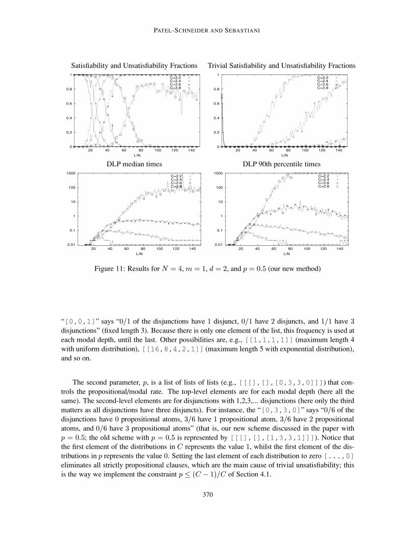
To illustrate the effects of varying C we generated formulae using Æ = 4, Ñ = ½, d = ½, andÔ = ¼:5, varying C from ¾:¾ to ¾:8. As shown in Figure 11, this produces an interesting set of tests.The difficulty levels can be set appropriately. Trivially unsatisfiable formulae do appear, but only

after the formulae become unsatisfiable anyway. Trivially unsatisfiable formulae do not influence

the difficulty of the test.

366



0

0.2

0.4

0.6

0.8

1

20 40 60 80 100 120 140 160 180 200

L/N

N=3N=4N=5N=6

0

0.2

0.4

0.6

0.8

1

20 40 60 80 100 120 140 160 180 200

L/N

N=3N=4N=5N=6


0.01

0.1

1

10

100

1000

20 40 60 80 100 120 140 160 180 200

L/N

N=3N=4N=5N=6

0.01

0.1

1

10

100

1000

20 40 60 80 100 120 140 160 180 200

L/N

N=3N=4N=5N=6


0.01

0.1

1

10

100

1000

20 40 60 80 100 120 140 160 180 200

L/N

N=3N=4N=5

0.01

0.1

1

10

100

1000

20 40 60 80 100 120 140 160 180 200

L/N

N=3N=4N=5

Figure 8: Results for C = ¿,Ñ = ½, d = ¾, and Ô = ¼:6 (our new method)

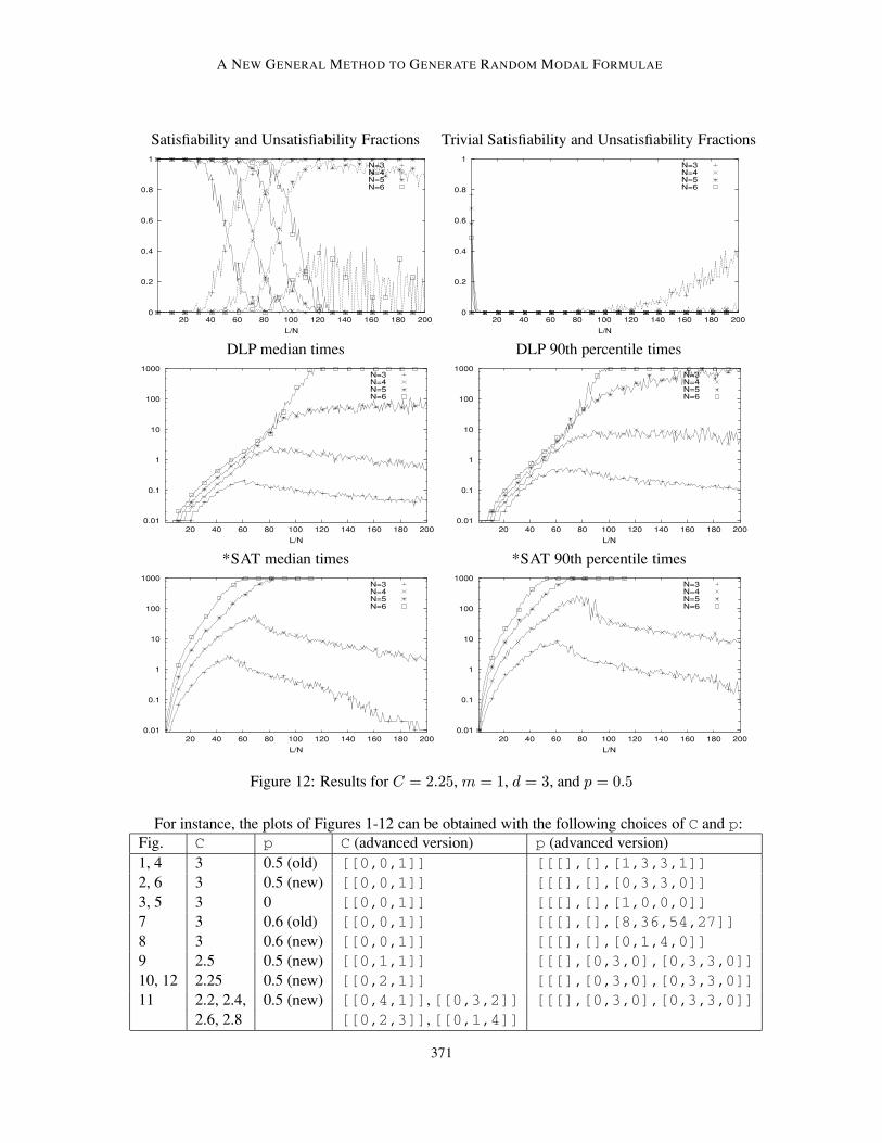
4.3.1 MODAL DEPTH ¿

Our method can be used to generate interesting test sets with modal depth d = ¿. This depth is notat all interesting with previous methods—either the formulae are immensely difficult, such as for

Ô = ¼, or the behavior is dominated by trivial unsatisfiability, such as for Ô = ¼:5.

For interesting levels of difficulty, we do have to reduce C to values below ¾:5. If C is much

larger, the formulae are too hard. However, with C ¾:5 we can produce interesting test sets, asshown in Figure 12. (The relevant asymmetry between the satisfiable and unsatisfiable rates curves

for Æ 5 is due to the high amount of tests exceeding the time limit.) Here the problems are hardeven for Æ 5 but doable, and there are no problems with trivially (un)satisfiable formulas.

367



0

0.2

0.4

0.6

0.8

1

20 40 60 80 100 120 140 160 180 200

L/N

N=3N=4N=5N=6

0

0.2

0.4

0.6

0.8

1

20 40 60 80 100 120 140 160 180 200

L/N

N=3N=4N=5N=6


0.01

0.1

1

10

100

1000

20 40 60 80 100 120 140 160 180 200

L/N

N=3N=4N=5N=6

0.01

0.1

1

10

100

1000

20 40 60 80 100 120 140 160 180 200

L/N

N=3N=4N=5N=6


0.01

0.1

1

10

100

1000

20 40 60 80 100 120 140 160 180 200

L/N

N=3N=4N=5N=6

0.01

0.1

1

10

100

1000

20 40 60 80 100 120 140 160 180 200

L/N

N=3N=4N=5N=6

Figure 9: Results for C = ¾:5,Ñ = ½, d = ¾, and Ô = ¼:5 (our new method)

Our method now allows us fine control of the difficulty of tests. To make a test easier, we can

just reduce the size of clauses by reducing the value(s) ofC , or increase the propositional probabilityÔ. This control was missing with the previous method, as C was restricted to integral value, and,

anyway, was always set to ¿ and making Ômuch different from ¼:¼ resulted in problems with trivialunsatisfiability for maximum modal depths greater than 1.

5. A new CNF¾Ñ generation method: advanced version

Actually, our generator is much more general than what we have described so far. We allow direct

specification of the probability distribution of the number of propositional atoms in a clause, and

368



0

0.2

0.4

0.6

0.8

1

20 40 60 80 100 120 140 160 180 200

L/N

N=3N=4N=5N=6N=7

0

0.2

0.4

0.6

0.8

1

20 40 60 80 100 120 140 160 180 200

L/N

N=3N=4N=5N=6N=7


0.01

0.1

1

10

100

1000

20 40 60 80 100 120 140 160 180 200

L/N

N=3N=4N=5N=6N=7

0.01

0.1

1

10

100

1000

20 40 60 80 100 120 140 160 180 200

L/N

N=3N=4N=5N=6N=7


0.01

0.1

1

10

100

1000

20 40 60 80 100 120 140 160 180 200

L/N

N=3N=4N=5N=6N=7

0.01

0.1

1

10

100

1000

20 40 60 80 100 120 140 160 180 200

L/N

N=3N=4N=5N=6N=7

Figure 10: Results for C = ¾:¾5, Ñ = ½, d = ¾, and Ô = ¼:5 (our new method)

allow the distribution to be different for each modal depth from the top level to d ½. We also allowdirect specification of the probability distribution for the number of literals in a clause at each modal

depth. Thus, the probability distribution for the number of propositional atoms depends on both the

modal depth and the number of literals in the clause.

5.1 Generalization: shaping the probability distributions.

The generator has two parameters to control the shape of formulae. The first parameter, C , is alist of lists (e.g., [[0,0,1]]) telling it how many disjuncts to put in each disjunction at each

modal level. Each internal list represents a finite discrete probability distribution. For instance, the

369



0

0.2

0.4

0.6

0.8

1

20 40 60 80 100 120 140

L/N

C=2.2C=2.4C=2.6C=2.8

0

0.2

0.4

0.6

0.8

1

20 40 60 80 100 120 140

L/N

C=2.2C=2.4C=2.6C=2.8


0.01

0.1

1

10

100

1000

20 40 60 80 100 120 140

L/N

C=2.2C=2.4C=2.6C=2.8

0.01

0.1

1

10

100

1000

20 40 60 80 100 120 140

L/N

C=2.2C=2.4C=2.6C=2.8

Figure 11: Results for Æ = 4,Ñ = ½, d = ¾, and Ô = ¼:5 (our new method)

“[0,0,1]” says “¼=½ of the disjunctions have ½ disjunct, ¼=½ have ¾ disjuncts, and ½=½ have ¿disjunctions” (fixed length 3). Because there is only one element of the list, this frequency is used at

each modal depth, until the last. Other possibilities are, e.g., [[1,1,1,1]] (maximum length 4

with uniform distribution), [[16,8,4,2,1]] (maximum length 5 with exponential distribution),

and so on.

The second parameter, Ô, is a list of lists of lists (e.g., [[[],[],[0,3,3,0]]]) that con-trols the propositional/modal rate. The top-level elements are for each modal depth (here all the

same). The second-level elements are for disjunctions with 1,2,3,... disjunctions (here only the third

matters as all disjunctions have three disjuncts). For instance, the “[0,3,3,0]” says “¼=6 of thedisjunctions have ¼ propositional atoms, ¿=6 have ½ propositional atom, ¿=6 have ¾ propositionalatoms, and ¼=6 have ¿ propositional atoms” (that is, our new scheme discussed in the paper with

Ô = ¼:5; the old scheme with Ô = ¼:5 is represented by [[[],[],[1,3,3,1]]]). Notice thatthe first element of the distributions in C represents the value ½, whilst the first element of the dis-tributions in Ô represents the value ¼. Setting the last element of each distribution to zero [...,0]eliminates all strictly propositional clauses, which are the main cause of trivial unsatisfiability; this

is the way we implement the constraint Ô Ć ½µ=C of Section 4.1.

370



0

0.2

0.4

0.6

0.8

1

20 40 60 80 100 120 140 160 180 200

L/N

N=3N=4N=5N=6

0

0.2

0.4

0.6

0.8

1

20 40 60 80 100 120 140 160 180 200

L/N

N=3N=4N=5N=6


0.01

0.1

1

10

100

1000

20 40 60 80 100 120 140 160 180 200

L/N

N=3N=4N=5N=6

0.01

0.1

1

10

100

1000

20 40 60 80 100 120 140 160 180 200

L/N

N=3N=4N=5N=6


0.01

0.1

1

10

100

1000

20 40 60 80 100 120 140 160 180 200

L/N

N=3N=4N=5N=6

0.01

0.1

1

10

100

1000

20 40 60 80 100 120 140 160 180 200

L/N

N=3N=4N=5N=6

Figure 12: Results for C = ¾:¾5,Ñ = ½, d = ¿, and Ô = ¼:5

For instance, the plots of Figures 1-12 can be obtained with the following choices of C and p:

Fig. C p C (advanced version) p (advanced version)

1, 4 3 0.5 (old) [[0,0,1]] [[[],[],[1,3,3,1]]

2, 6 3 0.5 (new) [[0,0,1]] [[[],[],[0,3,3,0]]

3, 5 3 0 [[0,0,1]] [[[],[],[1,0,0,0]]

7 3 0.6 (old) [[0,0,1]] [[[],[],[8,36,54,27]]

8 3 0.6 (new) [[0,0,1]] [[[],[],[0,1,4,0]]

9 2.5 0.5 (new) [[0,1,1]] [[[],[0,3,0],[0,3,3,0]]

10, 12 2.25 0.5 (new) [[0,2,1]] [[[],[0,3,0],[0,3,3,0]]

11 2.2, 2.4, 0.5 (new) [[0,4,1]], [[0,3,2]] [[[],[0,3,0],[0,3,3,0]]

2.6, 2.8 [[0,2,3]], [[0,1,4]]

371


1 function rnd CNF¾Ñ(d,m,L,N,p,C)

2 for i := 1 to Ä do /* generate Ä distinct random clauses */

3 repeat

4 CÐi := rnd clause(d,m,N,p,C);5 until is new(Cli); /* discards CÐ if it already occurs */

6 returnÎÄ

i=½ CÐi;

7 function rnd clause(d,m,N,p,C)

8 Ã := rnd length(d,C); /* select randomly the clause length */

9 È := rnd propnum(d,p,K); /* select randomly the prop/modal rate */

10 repeat

11 for j := 1 to È do /* generate P distinct random prop. literals */

12 Ðj := rnd sign()¡rnd atom(0,m,N,p,C);

13 for j := P+1 toÃ do /* generate K-P distinct random modal literals */

14 Ðj := rnd sign()¡rnd atom(d,m,N,p,C);

15 CÐ :=ÏÃ

j=½ Ðj ;

16 until no repeated atoms in(Cl); /* discards Cl if contains repeated atoms */

17 return ËÓÖØĆÐµ;

18 function rnd atom(d,m,N,p,C)

19 if d=0

20 then return rnd propositional atom(N); /* select randomly a prop. atom */

21 else

22 ¾Ö := rand box(m); /* select randomly an indexed box */

23 CÐ := rand clause(d-1,m,N,p,C);

24 return ¾ÖCÐ ;

Figure 13: Schema of the new CNF¾Ñrandom generator.

Our generator works as described in Figure 13. The function is new(Cli) checks if CÐi 6=CÐj; 8 j < i; rnd length(d,C) selects randomly the clause length according to the d · ½-th dis-tribution in C (e.g, if d is ½ and C is [[0,1,1][1,2][1]], it returns ½ with probability ½=¿and ¾ with probability ¾=¿); rnd propnum(d,p,K) selects randomly the number of propositional

atoms per clause È according to the [d · ½;Ã]-th distribution in Ô (e.g, if d is ½, Ã is ¾ and Ô is[[[],[0,1,0],[0,1,0,0]] [[1,0][0,1,0]]], it returns ½ deterministically); rnd signselects randomly either the positive or negative sign with equal probability; no repeated atoms in(Cl)

checks if the clause CÐ contains no repeated atom; Sort(Cl) returns the clause CÐ sorted accordingto some criterium; rnd propositional atom(N) selects with uniform probability one of the Æ propo-

sitional atoms Ai; rnd box(m) selects with uniform probability one of theÑ indexed boxes ¾Ö.

When eliminating duplicated atoms in a clause, we take care not to disturb these probabilities

by first determining the “shape” of a clause (rows 8-9 in Figure 13), and only then instantiating that

with propositional variables (rows 10-16 in Figure 13). If a clause has repeated atoms, either propo-

sitional or modal, the instantiation is rejected and another instantiation of the shape is performed.

372


If we did not take care in this way we would generate too few “small” atoms because there are

fewer small atoms than large atoms, resulting in a greater chance of rejecting small atoms because

of repetition.

The elimination of duplicated atoms in a clause is not only a matter of elimination of redundan-

cies, but also of elimination of a source of flaws. In fact, one might generate top-level clauses like

:::^ ´:¾½Á½ _ :A½µ _ :¾¾Á¾ _ :A¾µµ ^ :::, which would make the whole formula inconsistent.

Example 5.1 We try to guess a parameter set by which the new random generator can potentially

generate the following CNF¾Ñ formula ³:

´ :A¿ _ ¾½´:A4 _ :¾½A½µ _ ¾½´:A½ _ :¾½A¾µ µ ^´ :A½ _ ¾½Á¿ _ :¾½A¾µ _ :¾½´¾½:A4µ µ ^´ :A4 _ :¾½Á¾ _ ¾½:A½µ µ ^´ A½ _ :¾½´:¾½A4µ µ:

(2)

After a quick look we setÑ = ½, d = ¾, Æ = 4, Ä = 4. At top level we have 0 unary, 2 binary and2 ternary clauses; at depth 1 we have 2 unary and 4 binary clauses; at depth 2 we have only 6 unary

clauses. Thus, we can set

C = [[0,2,2],[2,4],[6]]. (3)

At top level there are no unary clauses (we represent this fact by the empty list “[]”), the 2 bi-

nary clauses have 1 propositional literal, and the 2 ternary clauses have 1 propositional literal; at

depth 1, the 2 unary clauses have 0 propositional literals, while the 4 binary clauses have 1 propo-

sitional literal. (There is no need to provide any information for depth 2, as all clauses are purely

propositional.) Thus, we can set

p = [[[],[0,2,0],[0,2,0,0]] [[2,0],[0,4,0]]]. (4)

The two expressions can then be normalized into:

C = [[0,1,1],[1,2],[1]]

p = [[[],[0,1,0],[0,1,0,0]] [[1,0],[0,1,0]]].(5)

Notice that any other setting of C , Ô obtained by changing the non-zero values in (5) into othernon-zero values, or turning zeros into non-zeros (but not vice versa!), will do the work, just with a

different probability. For instance, turning the first list in C into [1,1,1] allows for generating

also unary clauses at top level; anyway, with probability ´¾=¿µÄ the generator may still produce

formulae with only binary and ternary clauses at top level. ¾

As an illustration of our general method, we present a set of tests with Ñ = ½, d = ¿; 4,Æ = ¿; 4;, C =[[1,8,1]], and Ô =[[[1,0],[0,1,0],[0,1,1,0]]]. This set of testsintroduces a small fraction of single-literal clauses that contain a modal literal (except at the greatest

modal depth, where they contain, of course, a single propositional literal). The results of tests are

given in Figure 14. Again, trivial instances occur only out the interesting zone. Here we can generate

interesting test sets even with modal depth 4.

373



0

0.2

0.4

0.6

0.8

1

20 40 60 80 100 120 140

L/N

N,d=3,3N,d=4,3N,d=3,4N,d=4,4

0

0.2

0.4

0.6

0.8

1

20 40 60 80 100 120 140

L/N

N,d=3,3N,d=4,3N,d=3,4N,d=4,4


0.01

0.1

1

10

100

1000

20 40 60 80 100 120 140

L/N

N,d=3,3N,d=4,3N,d=3,4N,d=4,4

0.01

0.1

1

10

100

1000

20 40 60 80 100 120 140

L/N

N,d=3,3N,d=4,3N,d=3,4N,d=4,4

Figure 14: Results for DLP with d = ¿; 4, Æ = ¿; 4, C =[[1,8,1]],Ô =[[[1,0],[0,1,0],[0,1,1,0]]].

5.2 Varying the probability distributions with the depth

Our new method provides the ability to fine-tune the distribution of both the size and the propo-

sitional/modal rate of the clauses at every depth. This fine tuning results in a very large number

of parameters, and so far in this paper we have only investigated distributions that conform to the

scheme described above or ones that correspond to the 3CNF¾Ñ generation method previously used.

To give an example of how to vary the probability distributions with the nesting depth of the

clauses, we consider the case with d = 4; 5, Ñ = ½, Æ = ¿; 4; 5, C =[[1,8,1],[1,2]],Ô =[[[1,0],[0,1,0],[0,1,1,0]],[[1,0],[0,1,0]]]. The results of the tests aregiven in Figure 15.

The C parameter says that the probability distributions of the length of the clauses occurring at

nesting depth ¼ and ½ are [1,8,1] and [1,2] respectively. (When not explicitly specified, it is

considered the last distribution by default, as in the case of depth > ½.) Thus, the top-level clausesare on average ½=½¼ unary, 8=½¼ binary ½=½¼ ternary, while the clauses occurring at depth ½ areon average ½=¿ unary and ¾=¿ binary.

The Ô parameter says that the lists of probability distributions of the propositional/modal ratioat nesting depth ¼ and ½ are [[1,0],[0,1,0],[0,1,1,0]] and [[1,0],[0,1,0]] re-spectively. Thus, at every depth, unary clauses have no propositional literal and binary clauses have

374



0

0.2

0.4

0.6

0.8

1

0 20 40 60 80 100 120 140

L/N

N,d=3,4N,d=4,4N,d=5,4N,d=3,5N,d=4,5N,d=5,5

0

0.2

0.4

0.6

0.8

1

0 20 40 60 80 100 120 140

L/N

0

0.2

0.4

0.6

0.8

1

0 20 40 60 80 100 120 140

L/N

N,d=3,4N,d=4,4N,d=5,4N,d=3,5N,d=4,5N,d=5,5

0

0.2

0.4

0.6

0.8

1

0 20 40 60 80 100 120 140

L/N


0.01

0.1

1

10

100

1000

0 20 40 60 80 100 120 140

L/N

N,d=3,4N,d=4,4N,d=5,4N,d=3,5N,d=4,5N,d=5,5

0.01

0.1

1

10

100

1000

0 20 40 60 80 100 120 140

L/N

N,d=3,4N,d=4,4N,d=5,4N,d=3,5N,d=4,5N,d=5,5

Figure 15: Results for DLP with d = 4; 5, Ñ = ½, Æ = ¿; 4; 5, C =[[1,8,1],[1,2]],Ô =[[[1,0],[0,1,0],[0,1,1,0]],[[1,0],[0,1,0]]].

½ propositional and ½ modal literal. The top-level ternary clauses have either ½ or ¾ propositionalliterals, with equal probability.

Notice that at top level the distributions are identical to those of Figure 14, whilst at depth ½there are no more ternary clauses and a higher fraction of unary clauses. These slight modifica-

tions allow reasonable test sets with d = 5 and Æ = 5. Moreover, trivial instances have nearlydisappeared.

6. Generality of the method

We have already observed (Horrocks et al., 2000) that for normal modal logics, fromÃ´Ñµ upward,

there is no loss in the restriction to CNF¾Ñ formulae, as there is an equivalence between arbitrary

normal modal formulae and CNF¾Ñ formulae9 . We may wonder how well our generation tech-

nique covers the whole space of CNF¾Ñ formulae, and how well we can approximate a restricted

9. This holds for all modal normal logics from Ã´Ñµ upward, as the conversion works recursively on the depth of the

formula, from the leaves to the root, each time applying to sub-formulae the propositional CNF conversion and the

transformation

¾Ö

^

j

_

i

³ij =µ^

j

¾Ö

_

i

³ij ;

which preserves validity in such logics.

375


subclass of this space. Example 5.1 represents an instance of a very general property of our random

generation technique, which we present and discuss below.

Now we assume that the rnd CNF¾Ñ of Figure 13 is a “purely random” generator, i.e., it per-

forms all non-deterministic choices independently and in a pure random way. (Of course pseudo-

random generators only approximate this feature.) Moreover, with no loss of generality, we restrict

our discussion to CNF¾Ñ formulae which have no repeated clauses at top level and no repeated

atoms inside any clause at any level, and in which atoms are sorted within each clause, accord-

ing to the generic function Sort() of Figure 13. The former allows for considering only formulae

which are already simplified out; the latter allows for considering only one representative for each

class of formulae which are equivalent modulo order permutations. As discussed by Giunchiglia

et al. (2000), the latter allows for further simplifying subformulae like, e.g., ¾Á½_A¾µ_¾Á¾_A½µor ¾Á½ _A¾µ _ :¾Á¾ _ A½µ.

Let ³ be a sorted CNF¾Ñ formula of depth d and with Ä top-level clauses built on all the

propositional atoms fA½; :::AÆ g and on all the modal boxes f¾½; :::¾Ñg, which has no repeatedclause at top level and no repeated atoms inside any clause at any level. Then we can construct Cand Ô so that, for each i, j, Ö:

(a) the j-th element of the i-th sublist in C is non-zero if and only if there is a clause of length joccurring at depth i in ³, and

(b) the Ö · ½-the element of the j-th sub-sublist of the i-th sublist in Ô is non-zero if and only ifthere is a clause of length j occurring at depth i which contains Ö propositional literals.

One possible operative technique to build C and Ô works as follows. Initialize C as a list of d · ½sublists. Then, for every depth level i ¾ f¼; :::; dg, set the i-th sublist of C as follows:

(i) set the size Ã of the sublist as the maximum size of clauses occurring in ³ at depth i;

(ii) for all j ¾ f½; ::;Ãg, count the number of clauses of length j occurring in ³ at depth i, andappend the result to the sublist.

Initialize Ô as a list of d sublists of sub-sublists. Then, for every depth level i ¾ f¼; :::; d ½g, setthe i-th sublist of Ô as follows:

(i) look at C: set the size Ã of the sublist as the maximum size of clauses occurring in ³ at depthi;

(ii) for all j ¾ f½; ::;Ãg, generate the j-th sub-sublist as follows:

¯ look at C: if the number of clauses of length j occurring at depth i is non-zero, then setthe length Ð of the sub-sublist to j · ½, else set Ð to 0;

¯ for all Ö ¾ f¼; ::; Ð ½g, count the number of clauses of length j occurring in ³ at depth

i which have Ö propositional literals, and append the result to the sub-sublist.

Example 5.1 represents an instance of application of the above technique for construction C and Ôfrom ³. Notice that the C and Ô parameters not only verify points áµ and ´bµ above, but are suchthat the probability distributions mimic the actual number of occurrences of the different kinds of

clauses.

376


Theorem 6.1 Let rnd CNF¾Ñ be a purely random generator as in Figure 13. Let ³ be a sorted

CNF¾Ñ formula of depth d and with Ä top-level clauses built on all the propositional atoms in

fA½; :::AÆ g and on all the modal boxes in f¾½; :::¾Ñg, which has no repeated clause at top leveland no repeated atoms inside any clause at any level. Let C and Ô be built from ³ so that to verify

points áµ and ´bµ above. Let C ¼ and Ô¼ be obtained from C and Ô respectively by substituting somezero-values with some non-zero values. Then we have:

(i) rnd CNF¾Ñ(d,m,L,N,p,C) returns ³ with some non-zero probability È;

(ii) rnd CNF¾Ñ(d,m,L,N,p’,C’) returns ³ with some non-zero probability È ¼ È .

Proof The fully-detailed proof is reported in Appendix. Here we sketch the main steps.

The following facts come straightforwardly by induction on the structure of ³:

1. every propositional atom occurring in ³ at some depth i is returned with the same non-zeroprobability È½ by both rnd atom(0,m,N,p,C) and rnd atom(0,m,N,p’,C’);

2. every modal atom ¾ÚCÐ occurring in ³ at some depth i is returned with some non-zero proba-bility È¾ by rnd atom(d-i,m,N,p,C), and is returned with some non-zero probability È ¼

¾ È¾

by rnd atom(d-i,m,N,p’,C’);

3. every clause CÐ occurring in ³ at some depth i is returned with some non-zero probabilityÈ¿ by rnd clause(d-i,m,N,p,C), and is returned with some non-zero probability È ¼

¿ È¿ by

rnd clause(d-i,m,N,p’,C’).

Thus, every top level clause CÐk is returned by rnd clause(d,m,N,p,C) and rnd clause(d,m,N,p’,C’)with some non-zero probabilities Èk and È ¼

k respectively, being È ¼k Èk. From this fact, it comes

straightforwardly that ³ is returned by rnd CNF¾Ñ(d,m,L,N,p,C) and rnd CNF¾Ñ(d,m,L,N,p’,C’)

with some non-zero probabilities È and È ¼ respectively, being È ¼ È . Q.E.D.

Q.E.D.

From a theoretical viewpoint, Theorem 6.1 íµ shows that our generation technique is very

general, because, for every CNF¾Ñ formula ³, there exists a choice for the parameters s.t. a purelyrandom generator returns ³ with some non-zero probability È .

Of course, the choice criterium for C and Ô suggested by points áµ and ´bµ is not unique as,for example, any other setting obtained from it by turning zeros into non-zeros would match the

requirements. As an extreme case, we might think to do very general choices like

C = [[1,1,1,...],...] p = [[[[1,1],[1,1,1],[1,1,1,1]...]]]. (6)

which guarantee to have every possible CNF¾Ñ formula within a given bound in clause size with

non-zero probability. Anyway, Theorem 6.1 íiµ shows that, extending the number of non-zerosvalues, the probability of generating ³ decreases.

For instance, consider Example 5.1. Turning the first list in C of (5) into [1,1,1] would still

allow for generating the formula (2), but it would allow for generating also unary clauses at top level

with probability ½ ´¾=¿µÄ, which converges quickly to ½ with Ä.

Usually we are not interested in randomly generating one precise formula with some non-zero

probability —which would be rather small anyway— but rather to randomly generate a class of for-

mulae which are as similar as possible a given target class of formulae. Adding redundant non-zeros

would extend the range of shapes for formulae, extending the variance and lowering the resemblance

to the target class of formulae.

377


7. Discussion

7.1 The basic and the advanced method

Our new testing method can be used at two different levels, depending on the attitude —and on the

skills and experience— of the user.

In the basic usage the clause length C is represented by lists with either only one non-zero

element (e.g., [[0,0,1]], meaning “clause length ¾”) or only two adjacent non-zero elements(e.g., [[0,2,1]], meaning “clause length ¾ or ¿, with probability ¾=¿ and ½=¿ respectively”);similarly, the propositional/modal rate Ô is represented by lists with either only one non-zero element(e.g., [[[],[],[0,1,0,0]]], meaning “½ propositional literal per clause”) or only two non-zero adjacent elements (e.g., [[[],[],[0,3,2,0]]], meaning “either ½ or ¾ propositional

literals per clause, with probability ¿=5 and ¾=5 respectively”); the distributions do not vary withthe depth.

In the basic way the random generator is used as a “flawless”10 extension of the 3CNF¾Ñ

method of Giunchiglia and Sebastiani (1996), which allows for setting the clause length to either

fixed integer values or to non-integer average values. The number of parameters is kept relatively

small, so that to allow a coarse-grained coverage of a significant subspace with an affordable number

of tests.

In the advanced usage, it is possible to apply any finite probability distributions to both C and Ô;moreover, it is possible to use different distributions at different depths. This opens a huge amount

of possibilities, but requires some skills and experience from the user: the representation of sophis-

ticated multi-level distributions may be rather complicated, and may thus require some practice;

moreover, the usage of complex distributions requires some care, as the presence non-constant dis-

tributions in both clause length and propositional/modal rate may significantly enlarge the variance

of the features of the generated formulae, making the effects of the tests more unpredictable and

instance-dependent.

In order to guide the user, we provide some general suggestions for choosing the parameter sets

in a testing session. They come from both theoretical issues and our practical experience in using

the generator.

¯ Avoid generating purely propositional top-level clauses, that is, set p = [[...,0],...].

See Sections 4.1 and 5.1. If possible, avoid generating unary top-level clause, that is, set C

= [[0,...],...]). See also Section 7.5.

¯ In organizing a testing session, fix the parameter sets according to the following order and

directives.

(i) Fix d. With d=1 the search is mostly dominated by its propositional component, with

d>2 it tends to be dominated by its modal component. d=2 is typically a good start.

(ii) Fix m. m substantially partitions the problem into m independent problems. Increasing m,

the samples tend to be more likely-satisfiable. m=1 is typically a good start.

(iii) Set C. Increasing the top level values of C, the samples tend to be more likely-satisfiable

and the propositional component of search increases, so that the transition area moves

10. In the sense of “free from the flaw highlighted in the work by Hustadt and Schmidt (1999) and Giunchiglia

et al. (2000)”.

378


to the right and the hardness peaks grow. Average values in [¾:¼; ¿:¼] for the top leveldistributions of C are typically a good start.

(iv) Set p. Decreasing the top level values of p, the modal component of search increases.

For the the top level distributions of p, having on average half of top-level atoms propo-

sitional (that is, the Ô = ¼:5 of Section 4) is typically a good start.

(v) For each choice of the above parameters, increase N, starting from (at least) the maxi-

mum length in C, until the desired level of hardness is reached.

(vi) Make L vary within the satisfiability transition area.

¯ When dealing with C and p, focus on top-level clause distributions first. Small variations

of C and p at top level may cause big variations in hardness and satisfiability probability.

Variations at lower levels typically cause much smaller effects.

¯ Use convex distributions: e.g., [1,5,1] and [5,1,5] have the same mean value, but the

variance of the former is much smaller than that of the latter.

¯ Do keep L ranging in the satisfiability transition area: increasing L out of it, the fraction of

trivially unsatisfiable samples can become relevant. To determine the satisfiability transition

area, make a preliminary check with few samples per point (say, 10) using dichotomic search.

¯ Unlike N (and m), the parameters d, C, p make the formulas vary their shape. Thus, we

suggest to group together plots with the same d, C and p values and increasing N’s.

On the whole, the large number of parameters makes it impossible to cover the parameter space

in a reasonable amount of testing. However, just about any CNF¾Ñ formula shape can be generated

so that the method described in Section 6 can be used to produce random formulae reasonably

similar to some formula(e) of interest.

7.2 Comparison with the old 3CNF¾Ñ method

On the whole, the new method inherits all the features of the old 3CNF¾Ñ method.

Scalability: Increasing Æ , d (and also the average clause length inC) the difficulty of the generatedproblems scales up at will. Thus it is possible to compare how the performance of different

systems scale up with problems of increasing difficulty, for each source of difficulty (e.g.,

size, depth, etc.).

Valid vs. not-valid balance: The parameter Ä allows for tuning the satisfiability rate of the formulaat will. Moreover, it is always possible to choose Ä to generate testbeds with about a 50%-

satisfiable rate, which allows for the maximum uncertainty.

Termination: The new method allows for generating test sets of up to depth 3-4 which are run by

state-of-the-art systems in a reasonable amount of time.

Reproducibility: The results of each testbed are easy to reproduce because the generator’s code

and all the parameters’ values are made publicly available.

Parameterization: The random generation of CNF¾Ñ formulae is fully parametric.

379


Data organization: The most natural way to use the new random generator is to generate tests and

plot data by increasing values of one or two parameters. This allows for easy, quantitative and

qualitative evaluations of the performances of the different procedures under test.

Moreover, the new method improves the 3CNF¾Ñ method for the following features.

Representativeness: As stated in Section 6, CNF¾Ñ formulae represent all formulae in the normal

modal logics from Ã´Ñµ upward, as there is an equivalence-preserving way of converting all

modal formulae into CNF¾Ñ . From Theorem 6.1, the new method allows for a very fine-

grained sampling of the class of CNF¾Ñ formulae.

Difficulty: The random CNF¾Ñ formulae with d ¾ and Æ 4 provide challenging test sets forstate-of-the art procedures. CNF¾Ñ formulae with d 4 and Æ 9 can be well consideredas challenges for next-generation systems. (Of course, it is not a problem to generate easy

problems too.)

Control: The parameters Æ , d and C allow for controlling monotonically the difficulty of the test

set. (E.g., if you increase Æ , you are reasonably sure that your mean/median CPU time plots

will increase.) The parameter Ä allows for controlling the satisfiability rate. Monotonicity

allows for controlling one feature by simply increasing or decreasing one value, and thus for

eliminating uninteresting areas of the input space.

Modal vs. propositional balance: The size of the Kripke models spanned by the decision proce-

dures has increased exponentially with the higher modal depths reached by the new test sets;

moreover, the probability of repeated top-level atoms has dramatically reduced.11 Conse-

quently, unlike the tests by Hustadt and Schmidt (1999) and Giunchiglia et al. (2000) the

search is no longer dominated by the pure propositional component of reasoning, and the

empirical results show that a large number of modal successors are explored.

Finally, the new method completely removes or drastically reduces the effects of the following

problems.

Redundancy: Propositional and modal redundancy had already been eliminated in the last versions

of the 3CNF¾Ñ method (Giunchiglia et al., 2000). Moreover, the new method allows for

eliminating all strictly propositional clauses.

Triviality: The main cause of trivial unsatisfiability has been removed, so that trivially unsatisfiable

formulae have been relegated out of the transition areas in our experiments.

Artificiality: Our method allows the user to shape the test formulae so that to maximize the re-

semblance to the expected typical inputs of his/her system(s). Of course, this is done within

the limits imposed by randomness: the more irregular the typical input formulas, the higher

the variance of the randomly generated formulas, the lower their average resemblance to the

typical input formulas.

11. The number of possible distinct modal atoms increases hyper-exponentially with d (Horrocks et al., 2000).

380


Over-size: The new method allows for generating extremely hard problems with reasonable size.

It comes from the analysis of the resulting data that hard problems require very big amounts

of both search branches and modal successors generated, so that the search is not dominated

by parsing and data managing.

The generator presented by Horrocks and Patel-Schneider (2002), extends the 3CNF¾Ñ gener-

ator of Giunchiglia et al. (2000) too. However, our new generator allows for shaping the probability

distributions of both C and p, and for using different distributions at every depth level. In principle,

the generator of Horrocks and Patel-Schneider (2002) allows also for setting the probabilities ÒÔ

and ÒÑ by which propositional and modal atoms are negated. However, this feature is not used

very much—in the experiments by Horrocks and Patel-Schneider (2002) ÒÔ is always ¼:5 and ÒÑ

is different from ¼:5 only in one experiment— and adds nothing to the generality of the generator,

so that in our new generator we decided not to re-introduce it.

7.3 Comparison with QBF-based method

Before comparing our new CNF¾Ñ generation method with the QBF-based generation method, we

must notice that, so far, they have been used in different ways, corresponding to the two different

test techniques briefly summarized in Section 3.

¯ In the TANCS competition(s) (Massacci, 1999), the tests have been performed on single

data points, and the results are presented in the form of big tables, each entry consisting

of the number of successful solutions and in the rescaled geometrical mean CPU time for

such solutions. Two or more systems are compared according to their number of successful

solutions, considering the geometrical mean CPU time value only when the result is even.

This is due to the fact that a comparison between geometrical means is possible only if they

are computed on the same number of successful values, or, for a more accurate comparison,

on the same successful values.12 This method was chosen to guarantee the fairness of the

comparison between the competitors, which is the key requirement in a competition.

¯ In this paper instead, we have focused on highlighting both the qualitative and quantitative

behavior of the system(s). Thus we have preferred plots to tables, and we have preferred

representing percentiles CPU times rather than the number of successful solutions and their

geometrical mean times. In fact, the former does not require to distinguish between successful

and non-successful solutions.13 Thus, they are much more suitable for plotting, because

a comparison on geometrical means makes sense only for those data points with the same

number of successful solutions, which is very hard to follow in a plot.

Of course, both generators can be used in both ways. (See Heguiabehere and de Rijke (2001)

for some plots with the random QBF-based method.) Comparing the two approaches above in

organizing and presenting data is not one of the goals of this paper, so we restrict our analysis to the

generation methods, independently from how they have been used so far.

12. In case of tests exceeding the timeout, geometrical means are altered by the truncation introduced by the unsuccessful

solutions. Thus the geometrical mean makes sense only if calculated only on successful results.

13. If the percentage of successful solutions is greater or equal than É, then the value É-th percentile is not influenced

by the truncation of values introduced by timeouts, otherwise it is equal to the timeout value.

381


The QBF-based generation method of Massacci (1999) shares with our new CNF¾Ñ generation

method several features —in particular Scalability, Valid vs. not-valid balance, Termination, Re-

producibility, Parameterization, Data Organization, Difficulty, Modal vs. propositional bal-

ance, Redundancy and Triviality— for which considerations which are identical or analogous to

those for our new method hold, once we consider parameters Î ,D and C instead of parameters Æ ,

d and Ä. The following features instead deserve more discussion.

Control: The parameters Î andD allow for controlling monotonically the difficulty of the test set.

The parameter C allows for controlling the satisfiability rate. However, unlike the CNF¾Ñ

case, the main parameters of the QBF generator (e.g.,D and Î ) do not have a direct meaningwrt. the main characteristics of the resulting modal formulae like, e.g., the modal depth and

the number of propositional variables.

Representativeness: In general QBF formulae are good representatives for the whole class of

quantified boolean formulae, as there is a way to convert a generic quantified boolean formula

into QBF.14 (The randomly generated QBF formulae used by Massacci (1999) restrict to

those having a fixed amount of variables per alternation.) Nevertheless, the class of modal-

encoded QBF formulae restrict to those having candidate Kripke structures with the very

regular structure imposed by the QBF and/or binary search trees.

Artificiality: Unlike the CNF¾Ñ case, the main parameters of the QBF generator (e.g., D and Î )do not have a direct meaning wrt. the main characteristics of the resulting modal formulae.

Thus, it is hard to choose the parameters for the random QBF generator so that to resemble

expected typical inputs of the system(s).

Over-size: One final problem with random modal-encoded QBF formulae is size. Initial versions

of the translation method produced test sets in the 1GB range, which stressed too much the

data-storage and retrieval portion of the provers. (For example, running DLP on these formu-

lae resulted in a 1000s timeout without any significant search.) Although the encoding has

been significantly improved in this sense, the current versions still produce very large modal

formulae, mostly to constrain the Kripke structures.

Similar considerations have been very recently presented by Heguiabehere and de Rijke (2001).

On the whole, we believe that the QBF generation method is still appealing, and that the two

methods can co-exist in any empirical test session.

7.4 Complexity issues

From a purely theoretical viewpoint, it is remarked that modal-encoded QBF formulae can capture

the problems in ¦ÈD, while CNF¾Ñ formulae are “stuck at NP” (Massacci, 1999)15 . This statement

requires some clarification.

14. Notice that by “QBF” here we denote the class of prenex CNFQBF formulae, given by an alternation of quantification

variables ending with an existential one followed by a CNF propositional formula. The conversion works by lifting

quantifiers outside the formula and then converting into k-CNF [k-DNF] the matrix if the innest quantifier is an 9 [a 8,negating the result and pushing down the negation recursively]. The conversion is truth-preserving [truth-inverting].

15. More precisely, Massacci (1999) referred to the 3CNF¾Ñformulae of Giunchiglia et al. (2000). The statement holds

also for all the CNF¾Ñformulae.

382


First, test sets are necessarily finite, therefore it makes no sense to attribute to them a complexity

class. Thus, when speaking of complexity classes for test problems, we do not refer to test sets, but

rather to the infinite sets of formulae we could generate if we could have unbounded values for (at

least one of) the generation parameters. In particular, the statement above means that the infinite set

of QBF formulae with unbounded number of variables per alternation Î and bounded alternation

depth D is complete for ¦ÈD (Garey & Johnson, 1979), while the infinite set of CNF¾Ñ formulae

with bounded depth and unbounded number of propositional variables is in NP (Halpern, 1995).

Secondly, the alternation depth D and the variable number per alternation Î are not the “QBF-

analogous” of Ã´Ñµ’s modal depth and variable number respectively, as both the latter values for

the resulting modal formulae grow as Ç´D ¡ Î µ.16 In fact, QBF formulae with bounded alternationdepth D and unbounded number of variables per alternation Î give rise to modal formulae of both

unbounded depth and unbounded number of variables.

Finally, the “¦ÈD vs. NP” issue of Massacci (1999) is not a matter of generators, but rather a

matter of how such generators are used, and of how results are organized and presented. In fact,

so far random CNF¾Ñ testbeds have always been organized by fixing all the parameters except Ä(modal depth d included!) and making Ä vary. This choice, whose goal is to produce data plots

covering the satisfiability transition area, is what causes the testbed formulae to be “stuck at NP”.

To avoid this fact, one may want to make d vary and to fix all the other parameters, as Ã´Ñµ

satisfiability with unbounded depth and bounded number of propositional variables is PSPACE-

complete (Halpern, 1995).

7.5 Asymptotic behavior

Achlioptas et al. (1997) presented a study on the asymptotic behavior of random CSP problems.

They showed that, for most well-known random generation models (which did not reveal flaws in

empirical tests) the probability that problems are trivially unsatisfiable tends to 1 with Æ 7 ! ½,

Æ being the number of variables. Gent et al. (2001) lately explained this discrepancy between

theoretical and empirical results by showing that the above phenomenon happens with significant

probability only for values of Æ which are out of the reach of current CSP solvers.

The problem is due to the possible presence of (implicit) unary constraints causing some vari-

able’s value to be inadmissible. If this occurs with some non-zero probability, then with non-zero

probability some variable may have all its values inadmissible. This causes a “local” inconsistency

of the whole problem, which is very easily revealed by the solver. When Æ 7 ! ½, the probability

of not having such situation tends to zero. Analogous problems have been revealed with random

SAT problems generated with the constant probability generation model, as unary clauses are gen-

erated with non-zero probability (Mitchell et al., 1992), and with random QBF problems, as implicit

unit clauses, —i.e., clauses containing only one existential variable— are generated with non-zero

probability (Gent & Walsh, 1999). For the random k-SAT model, k ¾, such problem does not

occur (Friedgut, 1998; Achlioptas et al., 1997).

Our generation model is far more complicated to analyze than the models above. First, CNF¾Ñ

formulas have a much more complicated structure than random SAT, CSP and QBF formulas, in-

16. As we have already noticed (Horrocks et al., 2000), a better “QBF-analogous” of the modal depth is the total number

of universally quantified variables Í (Í = Î ¡ bD=¾c in our case). In fact, like modal Ã´Ñµ with bounded depth,

the class of QBF formulae with bounded Í is only complete in NP, as it is possible to “guess” a tree-like witness

with Ç´Í ¡ ¾Í µ nodes.

383


volving a much wider number of parameters. Second, unlike with the models discussed above, the

(constraints described by) CNF¾Ñ clauses are not picked in a uniform way, as the probability of

generating a given CNF¾Ñ atom ¾Ö varies strongly with its depth and shape, and it is typically

much smaller than that of generating a propositional atom Ai.17 Thus, developing a formal proba-

bilistic analysis for the asymptotic behavior of our model is out of the reach (and of the scope) of

this paper. However, we provide here some heuristic considerations.

The simplest case is when we do not allow the generation of unary clauses at top level, that is,

when C = [[0,...],...], so that we do not have explicit unary constraints. We may still have

implicit unary constraints like, e.g., Ái _ ¾Öµ ^ Ái _ :¾Öµ or ´¾i _ ¾Öµ ^ ´¾i _ :¾Öµ.Anyway, a simple heuristic consideration suggests that, given the big numbers of distinct CNF¾Ñ

modal atoms which may potentially be generated, such situations are more unlikely than that of

having implicit unit constraints like Ái _Ajµ ^ Ái _ :Ajµ in the standard 2-SAT model, which isfree from the asymptotic local inconsistency problem.

A more critical case is when we allow for the generation of unary clauses at top level, that

is, when C = [[x,...],...], Ü > ¼. In this case we can generate unary clauses, and thuslocal inconsistencies, with non-zero probability. Thus, a simple way to avoid this problem is to

restrict the values of C so that not to allow unary top-level clauses, that is, to always set C =

[[0,...],...]. Notice, however, that this hardly becomes a problem in practice if we re-

spect the condition described in Sections 4.1 and 5.1 of avoiding purely propositional top-level

clauses (that is, always set p = [[...,0],...]). In fact, given the big numbers of distinct

CNF¾Ñ modal atoms which may potentially be generated, the probability of having two contradic-

tory modal unit clauses ¾Ö, :¾Ö within the same formula becomes quickly negligible even withsmall depths.

Notice that here we have intentionally not considered “modal” implicit unary constraints like,

e.g., Ái _ µ ^ Ái _ µ, and being mutually inconsistent modal literals (e.g., = ¾Ö³½,

= :¾Ö´³½ _ ³¾µ). In fact, detecting such inconsistencies requires investigating recursively themodal successors, and therefore it is not “trivial”.

8. Conclusions and future work

As shown by the test sets above our new method, in its basic form, allows us to generate a wider

variety of problems covering more of the input space. We can better-tune the difficulty of problems

for various parameter values, including the first reasonable test sets for maximum modal depths

of ¾ and ¿. We can produce interesting scaling dimensions, varying more than just the number ofpropositional variables Æ . For example, we can now vary the propositional probability Ô or thesize of clauses C to vary the difficulty of interesting problems. As neither Ô nor C are restricted to

integral values, we have extremely fine control over the difficulty of test sets. Thus we can create

more interesting test sets where the satisfiable/unsatisfiable transition is explorable with current

decision procedures.

We have drastically reduced the influence of trivial unsatisfiability, which flawed the previous

CNF¾Ñmethodologies when Ô > ¼. We retain the desirable features of the previous CNF¾Ñmethodo-

logies. Our test sets are easy to reproduce and are not too large.

17. Again, we recall that the number of possible distinct CNF¾Ñatoms increases hyper-exponentially with the modal

depth d (Horrocks et al., 2000).

384


In our full methodology we have introduced the possibility of shaping the distribution of both

the size and the propositional/modal rate of the clauses. This can be done at each level of modal

depth. This allows for generating a much wider variety of problems, covering in principle the whole

input space. For instance, we have produced a full test set with d = 5 and Æ = 5 (Figure 15).

We have not moved closer to application data, as there are no significant direct applications

of modal decision procedures and thus no guidance for the sorts of inputs that would be close to

application inputs. In any case, we believe we have moved closer than ever to the possibility of

approximating given classes of input formulae.

There is still much work to be done using our generation methodology. We can produce more

test sets and try these test sets out on various modal decision procedures. We may also want to

uncover parameter settings where the full generality of our generation method is needed to produce

reasonable test sets.

References

Achlioptas, D., Kirousis, L. M., Kranakis, E., Krizanc, D., Molloy, M. S. O., & Stamatiou, Y. C.

(1997). Random constraint satisfaction: A more accurate picture. In Smolka, G. (Ed.), Prin-

ciples and Practice of Constraint Programming, No. 1330 in Lecture Notes in Computer

Science, pp. 107–120, Berlin. Springer.

Beckert, B., & Gore, R. (1997). Free variable tableaux for propositional modal logics. In Automated

Reasoning with Analytic Tableaux and Related Methods: International Conference Tab-

leaux’97, No. 1227 in Lecture Notes in Artificial Intelligence, pp. 91–106, Berlin. Springer.

Cadoli, M., Giovanardi, A., & Schaerf, M. (1998). An algorithm to evaluate quantified Boolean

formulae. In Proceedings of the 15th National Conference on Artificial Intelligence (AAAI-

98), pp. 262–267, Menlo Park, CA. AAAI Press.

Friedgut, E. (1998). Sharp thresholds of graph properties, and the k-sat problem. Journal of the

American Mathematical Society, 12(4), 1017–1054.

Garey, M. R., & Johnson, D. S. (1979). Computers and Intractability: A Guide to the Theory of

NP-Completeness. W. H. Freeman, New York.

Gent, I. P., MacIntyre, E., Prosser, P., Smith, B. M., & Walsh, T. (2001). Random constraint satis-

faction: Flaws and structure. Journal of Constraints, 6(4), 345–372.

Gent, I. P., & Walsh, T. (1999). Beyond NP: The QSAT phase transition. In Proceedings of the

Sixteenth National Conference on Artificial Intelligence and the Eleventh Innovative Applica-

tions of Artificial Intelligence Conference (AAAI-99), pp. 648–653, Menlo Park, CA. AAAI

Press.

Giunchiglia, E., Giunchiglia, F., Sebastiani, R., & Tacchella, A. (2000). SAT vs. Translation based

decision procedures for modal logics: a comparative evaluation. Journal of Applied Non-

Classical Logics, 10(2), 145–172.

Giunchiglia, E., Giunchiglia, F., & Tacchella, A. (2002). SAT based decision procedures for classical

modal logics. Journal of Automated Reasoning, 28, 143–171.

Giunchiglia, F., & Sebastiani, R. (1996). Building decision procedures for modal logics from propo-

sitional decision procedures - the case study of modal K. In Proceedings of the Thirteenth

385


Conference on Automated Deduction, No. 1104 in Lecture Notes in Artificial Intelligence, pp.

583–597, Berlin. Springer.

Giunchiglia, F., & Sebastiani, R. (2000). Building decision procedures for modal logics from propo-

sitional decision procedures - the case study of modal K(m). Information and Computation,

162(1/2), 158–178.

Haarslev, V., & Moller, R. (2001). RACER system description. In Proceedings of the Interna-

tional Joint Conference on Automated Reasoning, IJCAR’2001, Vol. 2083 of Lecture Notes

in Computer Science, pp. 701–705, Siena, Italy. Springer.

Halpern, J. Y. (1995). The effect of bounding the number of primitive propositions and the depth of

nesting on the complexity of modal logic. Artificial Intelligence, 75(3), 361–372.

Halpern, J. Y., & Moses, Y. (1992). A guide to the completeness and complexity for modal logics

of knowledge and belief. Artificial Intelligence, 54(3), 319–379.

Heguiabehere, J., & de Rijke, M. (2001). The random modal QBF test set. In IJCAR’2001 Workshop

on Issues in the Design and Experimental Evaluation of System for Modal and Temporal

Logics, pp. 58–67.

Heuerding, A., Jager, G., Schwendimann, S., & Seyfreid, M. (1995). Propositional logics on the

computer. In Baumgartner, P., Hahnle, R., & Posegga, J. (Eds.), Automated Reasoning with

Analytic Tableaux and Related Methods: International Conference Tableaux’95, No. 918 in

Lecture Notes in Artificial Intelligence, pp. 310–323, Berlin. Springer.

Heuerding, A., & Schwendimann, S. (1996). A benchmark method for the propositional modal

logics K, KT, S4.. Tech. rep. IAM-96-015, University of Bern, Switzerland.

Horrocks, I. (1998). Using an expressive description logic: FaCT or fiction?. In Cohn, A. G., Schu-

bert, L., & Shapiro, S. C. (Eds.), Principles of Knowledge Representation and Reasoning:

Proceedings of the Sixth International Conference (KR’98), pp. 636–647. Morgan Kaufmann

Publishers, San Francisco, California.

Horrocks, I., & Patel-Schneider, P. F. (2002). Evaluating optimised decision procedures for propo-

sitional modal Ã´Ñµ satisfiability. Journal of Automated Reasoning, 28(2), 173–204.

Horrocks, I., Patel-Schneider, P. F., & Sebastiani, R. (2000). An analysis of empirical testing for

modal decision procedures. Logic Journal of the IGPL, 8(3), 293–323.

Hustadt, U., & Schmidt, R. A. (1999). An empirical analysis of modal theorem provers. Journal of

Applied Non-Classical Logics, 9(4), 479–522.

Hustadt, U., Schmidt, R. A., &Weidenbach, C. (1999). MSPASS: Subsumption testing with SPASS.

In Lambrix, P., Borgida, A., Lenzerini, M., Moller, R., & Patel-Schneider, P. (Eds.), Proceed-

ings of the 1999 International Workshop on Description Logics (DL’99)., pp. 136–137.

Massacci, F. (1999). Design and results of Tableaux-99 non-classical (modal) system competition.

In Automated Reasoning with Analytic Tableaux and Related Methods: International Con-

ference Tableaux’99, No. 1617 in Lecture Notes in Artificial Intelligence, pp. 14–18, Berlin.

Springer.

Mitchell, D., Selman, B., & Levesque, H. (1992). Hard and easy distributions of SAT problems.

In Proceedings of the Tenth National Conference on Artificial Intelligence, pp. 459–465, San

Jose, California. American Association for Artificial Intelligence.

386


Patel-Schneider, P. F. (1998). DLP system description. In Franconi, E., Giacomo, G. D., MacGre-

gor, R. M., Nutt, W., Welty, C. A., & Sebastiani, F. (Eds.), Collected Papers from the Inter-

national Description Logics Workshop (DL’98), pp. 87–89. Available as CEUR-WS/Vol-11

from http://SunSITE.Informatik.RWTH-Aachen.DE/Publications/CEUR-WS.

Patel-Schneider, P. F., & Sebastiani, R. (2001). A new system and methodology for generating ran-

dom modal formulae. In Proceedings of the International Joint Conference on Automated

Reasoning, IJCAR’2001, Vol. 2083 of Lecture Notes in Computer Science, pp. 464–468,

Siena, Italy. Springer.

Pitt, J., & Cunningham, J. (1996). Distributed modal theorem proving with KE. In Minglioli,

P., Moscato, U., Mindici, D., & Ornaghi, M. (Eds.), Automated Reasoning with Analytic

Tableaux and Related Methods: International Conference Tableaux’96, No. 1071 in Lecture

Notes in Artificial Intelligence, pp. 160–176, Berlin. Springer.

Tacchella, A. (1999). *SAT system description. In Lambrix, P., Borgida, A., Lenzerini, M., Moller,

R., & Patel-Schneider, P. (Eds.), Proceedings of the 1999 International Workshop on Descrip-

tion Logics (DL’99)., pp. 142–144.

Appendix: Fully-detailed proof of Theorem 6.1

Theorem 6.1 Let rnd CNF¾Ñ be a purely random generator as in Figure 13. Let ³ be a sorted

CNF¾Ñ formula of depth d and with Ä top-level clauses built on all the propositional atoms in

fA½; :::AÆ g and on all the modal boxes in f¾½; :::¾Ñg, which has no repeated clause at top leveland no repeated atoms inside any clause at any level. Let C and Ô be built from ³ so that to verify

points áµ and ´bµ of Section 6. Let C ¼ and Ô¼ be obtained from C and Ô respectively by substitutingsome zero-values with some non-zero values. Then we have:

(i) rnd CNF¾Ñ(d,m,L,N,p,C) returns ³ with some non-zero probability È;

(ii) rnd CNF¾Ñ(d,m,L,N,p’,C’) returns ³ with some non-zero probability È ¼ È .

Proof The proof works by induction on the structure of ³. First, we prove that:

1. every propositional atom occurring in ³ at some depth i is returned with the same non-zeroprobability È½ by both rnd atom(0,m,N,p,C) and rnd atom(0,m,N,p’,C’);

2. every modal atom ¾ÚCÐ occurring in ³ at some depth i is returned with some non-zero proba-bility È¾ by rnd atom(d-i,m,N,p,C), and is returned with some non-zero probability È ¼

¾ È¾

by rnd atom(d-i,m,N,p’,C’);

3. every clause CÐ occurring in ³ at some depth i is returned with some non-zero probabilityÈ¿ by rnd clause(d-i,m,N,p,C), and is returned with some non-zero probability È ¼

¿ È¿ by

rnd clause(d-i,m,N,p’,C’).

From point 3. we have that every top level clause CÐk is returned by rnd clause(d,m,N,p,C) and

rnd clause(d,m,N,p’,C’) with some probabilities Èk and È ¼k respectively, being È ¼

k Èk. As ³

387


has no repeated clause, recalling a property of probabilities we have:

È =

È½¡´È¾ · È½È¾ · È¾

½È¾ · : : :µ¡´È¿ · ´È½ · È¾µÈ¿ · ´È½ · È¾µ

¾È¿ · : : :µ¡: : :´ÈÄ · ´È½ · : : :· ÈÄ ½µÈÄ · ´È½ · : : :· ÈÄ ½µ

¾ÈÄ · : : :µ

(7)

=ÄY

k=½

½X

i=¼

´k ½X×=½

È×µi ¡ Èk

!(8)

=

ÄYk=½

Èk

½ Èk ½

×=½ È×

: (9)

Notice that (8) is strictly monotonic in all its components. Thus, È ¼ È .Now we need to prove points 1, 2 and 3.

1. Let Ak be a propositional atom in fA½; :::; AÆ g occurring in ³ at depth i, for some i d.Then both rnd atom(0,m,N,p,C) and rnd atom(0,m,N,p’,C’) invoke rnd propositional atom(N),

which returns Ak with probability È½ = ½=Æ .

2. Let ¾ÚCÐ be a boxed clause occurring in ³ at depth i, for some i < d and Ú Ñ. Then theclause CÐ occurs in ³ at depth i· ½. (Notice that i < d instead of i d: ¾ÚCÐ cannot occurin ³ at depth d, because d is the maximum depth of ³.)

(i) By inductive hypothesis, it follows from point 3. that CÐ is returned with some non-zeroprobability È¿ by rnd clause(d-i-1,m,N,p,C). As i < d, rnd atom(d-i,m,N,p,C) invokesrand box(m) ¡ rand clause(d-i-1,m,N,p,C), which returns ¾ÚCÐ with the non-zero prob-ability È¾ = ½=Ñ ¡ È¿.

(ii) By inductive hypothesis, it follows from point 3. that CÐ is returned with some non-zero probability È ¼

¿ È¿ by rnd clause(d-i-1,m,N,p’,C’). rnd atom(d-i,m,N,p’,C’) in-

vokes rand box(m) ¡ rand clause(d-i-1,m,N,p’,C’), which returns ¾ÚCÐ with the non-zero probability È ¼

¾ = ½=Ñ ¡ È ¼¿. Thus, È ¼

¾ È¾.

3. Let CÐ be a clause with length j and Ö j propositional literals, which occurs in ³ at depth

i, for some i d. As ³ is sorted, CÐ is represented as ËÓÖØ´ ½ _ ::: _ Ö _ ½ _ ::: _ j Öµ,where ½; :::; Ö denote propositional literals and ½; :::; j Ö denote modal literals.

(i) By inductive hypothesis, it follows from point 1. that each propositional literal k is

returned with some non-zero probability ¼:5 ¡ È½;k by rnd sign() ¡ rnd atom(0,m,N,p,C),and it follows from point 2. that each modal literals Ð is returned with the non-zero

probability ¼:5 ¡ È¾;Ð by rnd sign() ¡ rnd atom(d-i,m,N,p,C).

By construction of C , the j-th element of the i-th sublist in C is non-zero; thus, j isreturned with some non-zero probability Èj by rnd length(d-i,C).

By construction of Ô, the Ö·½-the element of the j-th sub-sublist of the i-th sublist in Ô isnon-zero; thus, Ö is returned with some non-zero probability ÈÖjj by rnd propnum(d,p,j).

18

18. Notice that ÈÖjj is a conditioned probability, that is, the probability of having Ö propositional literal provided the

clause has j literals. This matches the fact that j is an input in rnd propnum(d,p,j).

388


Similarly to (9), ³ has no repeated atoms inside any clause, so that CÐ is returned byrnd clause(d-i,m,N,p,C) with the non-zero probability

È¿ = Èj ¡ ÈÖjj ¡ ´¼:5µj ¡ÖY

k=½

È½;k

½ Èk ½

×=½ È½;×

¡

j ÖYÐ=½

È¾;Ð

½ ÈÐ ½

Ø=½ È¾;Ø

: (10)

As with (9), the expression on the right in (10) is strictly monotonic in all its terms Èj ,

ÈÖjj , È½;k ’s, È¾;Ð ’s within the domain of definition.

(ii) By inductive hypothesis, it follows from point 1. that each propositional literal k

is returned with some non-zero probability ¼:5 ¡ È ¼½;k ¼:5 ¡ È½;k by rnd sign() ¡

rnd atom(0,m,N,p’,C’), and it follows from point 2. that each modal literals Ð is re-

turned with some non-zero probability ¼:5 ¡ È ¼¾;Ð ¼:5 ¡ È¾;Ð by rnd sign() ¡ rnd atom(d-

i,m,N,p’,C’).

By construction of C and C ¼, the j-th element of the i-th sublist in C ¼ is non-zero; thus,

j is returned with some non-zero probability È ¼j by rnd length(d-i,C’). By construction

of C ¼ from C , È ¼j Èj .

By construction of Ô and Ô¼, the Ö · ½-the element of the j-th sub-sublist of the i-thsublist in Ô is non-zero; thus, Ö is returned with some non-zero probability È ¼

Öjj by

rnd propnum(d,p,j). By construction of Ô¼ from Ô, È ¼Öjj ÈÖjj .

As³ has no repeated atoms inside any clause, it follows thatCÐ is returned by rnd clause(d-i,m,N,p’,C’) with the non-zero probability

È ¼¿ = È ¼

j ¡ È ¼Öjj ¡ ´¼:5µj ¡

ÖYk=½

È ¼½;k

½ Èk ½

×=½ È ¼½;×

¡

j ÖYÐ=½

È ¼¾;Ð

½ ÈÐ ½

Ø=½ È ¼¾;Ø

: (11)

Because of the strict monotonicity of (10) and (11), we have that È ¼¿ È¿.

Q.E.D.

389

Documents

A N e w Ge n e r al M e th od to Ge n e r ate R an d om M ... · In Section 2 we recall a lis t o f desira ble fea tures for g ood test se ts. ... the advanced version of ou r metho