Analysis of Retinotopic Maps inExtrastriate Cortex

Martin I. Sereno, Colin T. McDonald, and John M.Allman

Cognitive Science, University of California at SanDiego, La JoUa, California 92093-0515 and Division ofBiology, California Institute of Technology, Pasadena,California 92115

Two new techniques for analyzing retinotopic maps—arrow diagrams and visual field sign maps—are dem-onstrated with a large electrophysiological mappingdata set from owl monkey extrastriate visual cortex. Anarrow diagram (vectors indicating receptive field cen-ters placed at cortical coordinates) provides a morecompact and understandable representation of retino-topy than does a standard receptive field chart (accom-panied by a penetration map) or a double contour map(e.g., isoeccentricity and isopolar angle as a functionof cortical x, y-coordinates). None of these three rep-resentational techniques, however, make separate ar-eas easily visible, especially in data sets containingnumerous areas with partial, distorted representationsof the visual hemrfield. Therefore, we computed visualfield sign maps (non-mirror-image vs mirror-image vi-sual field representation) from the angle between thedirection of the cortical gradient in receptive field ec-centricity and the cortical gradient in receptive fieldangle for each small region of the cortex. Visual fieldsign is a local measure invariant to cortical map ori-entation and distortion but also to choice of receptivefield coordinate system. To estimate the gradients, wefirst interpolated the eccentricity and polar angle dataonto regular grids using a distance-weighted smooth-ing algorithm. The visual field sign technique providesa more objective method for using retinotopy to outlinemultiple visual areas. In order to relate these arrowand visual field sign maps accurately to architectonicfeatures visualized in the stained, flattened cortex, wealso developed a deformable template algorithm forwarping the photograph-derived penetration map usingthe final observed location of a set of marking lesions.

Over half of the neocortex in primates consists of vi-sual areas, many of which are retinotopically orga-nized (for reviews, see Felleman and Van Essen, 1991;Kaas and Krubitzer, 1991; Sereno and Allman, 1991).The region of cortex involved, however, is large, andthere is substantial variability among species andamong individual animals of a species. Even well-de-fined areas like primary visual cortex (VI) and themiddle temporal area (MT) show variability in theirlocation, shape, size, and appearance (on MT in NewWorld monkeys, see, e.g., Tootell et al., 1985; Fioraniet al., 1989). Since the majority of visual areas are notgraced with the convenient suite of easily distinguish-able features that characterize VI and MT (e.g., prom-inent myeloarchitectonic borders, nearly complete,not-too-distorted, topological maps of the hemiretina),it has proved quite difficult to define their boundariesconvincingly. Several different naming schemes havepersisted for a number of the areas beyond VI, V2,and MT.

Visual areas in the cortex are ideally defined on thebasis of converging criteria (Allman and Kaas, 1971,1974, 1975, 1976; Van Essen, 1985). These include vi-suotopic organization, architectonic features, connec-tion patterns, and physiological properties. It is virtu-ally impossible, however, to obtain detailedinformation about all of these criteria for multiple vi-sual areas in a single animal. In the following report,we have focused on the first two criteria—visuotopyand architectonics. By concentrating on obtaininglarge numbers of recording sites in each animal, wehave been able to delineate much more clearly thecomplex and variable mosaic of visual areas in primatedorsal, lateral, and ventral extrastriate cortex.

In the present article, we begin by describing ourtechniques for recording visual receptive fields froma large number of locations in each animal. In the pro-cess of analyzing these large data sets, it became clearthat the standard technique for illustrating retinoto-py—a numbered penetration site chart with corre-spondingly numbered receptive field charts—wasmuch too unwieldy to handle multiple, partial visualfield representations involving hundreds of sites. Weneeded to find a tractable way to view the entire dataset for a single animal, not the least to avoid the temp-tation to extract the small portions of the data set thatcan often be found to support a simple story.

We describe two new methods for representing

Cerebral Cortex Nov/Dec 1994;6:601-620; 1047-3211/94/54.00

large retinotopic mapping data sets in an interpretableway—arrow diagrams and visual field sign maps. Wefirst illustrate conventional numbered receptive field/penetration plots and then show how arrow (vectorfield) diagrams make it possible to view the same dataset much more compactly and understandably. Sec-ond, we describe a deterministic distance-weighted al-gorithm for interpolating receptive field eccentricity,angle, and diameter data onto regular grids so that wecan generate isoeccentricity, isopolar angle, and iso-diameter contour plots. Third, we describe how tomake a visual field sign map (local mirror-image vsnon-mirror-image transformation of the visual field)from the interpolated isoeccentricity and isopolar an-gle grids. This technique brings out relations that areoften subtle in an arrow diagram and completelyopaque in a raw receptive field plot. Finally, we de-velop an iterative algorithm for warping an x-y pen-etration map derived from a recording photographonto the stained, physically flattened cortex usingmarker lesions. This allows us to align our mappingdata more accurately with anatomical landmarks.

The overall picture of retinotopy in primate extra-striate visual cortex that we arrived at was substan-tially more complex than we had anticipated. In aforthcoming companion article we use the techniquesdeveloped here to analyze retinotopy and architecton-ic features of dorsolateral extrastriate cortical areas inthe owl monkey. A detailed discussion of the 600+point case illustrated here will be contained in thatreport. In a third companion article we will examineventrolateral extrastriate areas in the owl monkey.

Portions of this work have been presented in ab-stract form (Sereno et al., 1986, 1987, 1993).

Materials and MethodsThe analytical techniques described in this articlewere developed in the course of a long series ofchronic and acute electrophysiological mapping ex-periments on anesthetized owl monkeys (Aotus tri-virgatus). They will be demonstrated by a single, ex-tensive acute mapping experiment, which isdescribed below. Our chronic mapping proceduresand variations in our acute procedures will be de-scribed in the forthcoming companion articles.

Acute Mapping Experiment ProceduresThe animal was deeply anesthetized and a large cra-niotomy made. A rod was cemented to the skull usingseveral small stainless steel bone screws and Grip den-tal acrylic cement under full aseptic conditions to al-low the animal's head to be fixed without pressurepoints. The animal was positioned for recording in thenatural crouched resting posture of the owl monkeyin a special!)' designed monkey chair (owl monkeyslack ischial callosities and cannot sit comfortably forextended periods on a standard macaque monkeychair). The animal was tilted somewhat to keep thesurface of the cortex close to horizontal. The dura wasretracted and the cortex was covered with a pool ofwarm sterile silicone oil. The vascular pattern of theexposed cortex was then photographed. The animal's

body temperature was monitored with a rectal probeand maintained with a warm water pad, and the ani-mal was given 5% dextrose in saline intravenously toprevent dehydration. Care was taken to express urineaccumulated in the bladder. Anesthesia was main-tained with additional doses of ketamine (3-5 mg/kg/hr, i.m., or as needed to suppress muscular or heartrate response to stimuli). The depth of anesthesia ofthe unparalyzed animal was monitored continuouslyby the person manipulating the electrode. Triflupro-mazine was given initially (3-6 mg/kg, i.m.) and after-ward in smaller doses at 10-15 hr intervals (2 mg/kg,i.m.) because of its longer resident time. Trifluproma-zine potentiates the effects of ketamine The animalmonocularly viewed a translucent, dimly back-lit plas-tic hemisphere 28.5 cm in diameter (1° of visual angleequals 5 mm along hemisphere surface) that was cen-tered on the open contralateral eye.

A stepping motor microdrive was positioned in thex-y plane with a manual micromanipulator while ob-serving the brain surface through a dissecting micro-scope. Each electrode penetration was first marked onthe enlarged photograph (20X) of the vascular pat-tern on the cortical surface with the electrode tiptouching the pial surface. A glass-coated platinum-irid-ium microelectrode with 10-40 \x.m tip exposures wasthen driven perpendicularly into the cortex with thestepping motor microdrive (designed by Herb Adams,California Institute of Technology) to depths of ap-proximately 700 \im. Up to 25 penetrations per mm2

were made in regions where receptive field positionchanged rapidly. The x, y-location of a recording siteas marked on the cortical surface photograph is sub-ject to small errors due to difficulties in triangulatingfrom blood vessel landmarks in the microscope image.However, since the smallest vessels on the pial surfaceare typically separated by only 100-200 jun, locationerrors were probably restricted to within a 50 imradius of the true location in the x-y plane. With thesetechniques, it was possible to record more than 600receptive fields in one very long session (90 hr). Smallelectrophysiological lesions (10-20 |xA for 10 sec)were made before the end of the experiment to iden-tify individual recording sites.

Visual StimulationThe cornea was anesthetized with a long acting localanesthetic (0.7% dibucaine HC1 dissolved in contactlens wetting solution). The pupil was dilated with Cy-clogyl (1%). A thin ring machined to the contours ofthe large owl monkey eye was then cemented to themargin of the anesthetized cornea with a small drop(—10 \L\) of Histoacryl cyanoacrylate tissue cement.An appropriate contact lens was placed over the cor-nea (the diameter of the ring was slightly larger thanthe contact) to prevent drying during the course ofthe experiment and to bring the eye into focus. Thistechnique provides excellent stability because of thelarge size of the owl monkey eye and the poor me-chanical advantage of the posteriorly inserting eyemuscles in this nocturnal animal. Paralysis is thus

602 Retinotopic Maps in Extrastriate Cortex • Sereno et al

avoided making it easier to monitor and maintain theanesthetic state of the animal.

At the beginning of the experiment, the blind spotand four other widely separated retinal blood vessellandmarks were plotted on the plastic hemisphere bybackprojecting their images with an ophthalmoscope.These landmarks were checked repeatedly during theexperiment. Gaze remained fixed to within the accu-racy of our backprojection technique (si°) for theduration of the 90 hr experiment. Many points aroundthe circumference of each receptive field were testedcarefully to determine its extent using backprojectedlight and dark spots, bars, and texture patterns whilelistening to an audio monitor. We plotted the positionof the response field for single neurons or small clus-ters of neurons. The hemisphere was dimly lit to avoidspurious responses due to light scatter. Receptivefields and retinal landmarks were copied onto tracingpaper made into a hemisphere by small, taped radialfolds after ever)' 30-50 had been plotted so that wecould clear the plastic hemisphere to avoid confusion

Histology and Cortical Flat-MountsAt the end of the experiment, the animal was deeplyanesthetized with Nembutal (100 mgAg, i.v.) and per-fused through the heart with buffered saline. We im-mediately removed the unfixed brain and physicallyflattened the cortex (Olavarria and Van Sluyters, 1985;Tootell et al., 1985) by gently dissecting away thewhite matter with dry Q-Tips. In the later stages ofthis process, the cortex was supported, pial surfacedown, on moist filter paper. A cut in the fundus of thecalcarine sulcus and two smaller cuts in the cortex atthe anterior ends of the sylvian sulcus and the supe-rior temporal sulcus were made to allow the cortexto lie flat It was held in fixative without sucrose be-tween large glass slides under a small weight for sev-eral hours (sucrose tends to cause the tissue to slipout from between the slides). The tissue was kept freefloating in fixative overnight, and then soaked in 30%sucrose solution the following day.

The flattened cortex was sectioned in one pieceparallel to cortical laminae at 50 p.m on a large freez-ing microtome stage. A built-up block of ice was firstshaved flat with the microtome knife. The flattenedcortex was held on the underside of a moistened glassslide and then attached, pial surface down, to the cutice surface with a thin coat of Tissue-Tek compound.Overly rapid initial freezing of the tissue can trappockets of air in between the ice and the tissue. Dur-ing sectioning, the knife often lifts these regions fromthe block, destroying them as it cuts deeply into thetissue. To avoid this, the block temperature was firstraised to approximately - 15°C; this provides 5-10 secto exclude air bubbles by pressing and tapping on theoverlying slide while the tissue freezes. With tech-nique, it was often possible to recover every section,including the most superficial, which contains mainlyblood vessels. By aligning this section with deeper sec-tions using radial blood vessels, it was possible to drawadditional correspondences between the stained tis-sue and the penetration photograph. Every section

Visual Field Visual Cortex

Figure 1. Seven receptive field parameters. The location of trie recording siteis measured from the penetration photograph {x, v), the center of the recep-tive field is defined by its eccentricity and angle (r, 0), and the receptive fieldshape is parameterized by the length, width, and angle of the best-fittingellipse (/, w, $). An arrow diagram (see Figs. 5, 6) is constructed by placinga sealed copy of the arrow from the center of gaze to the receptive fieldcenter {thick arroWi at the x, y-posttion on the cortex from which that re-ceptive Meld was recorded. A receptive field on the horizontal meridian ofthe left hemifield is conventionally labeled with an angle of 0°

was stained using the Gallyas (1979) technique afterdrying mounted sections in air for 2 d (longer delaysresult in light, irregular staining).

Digitization of Cortical Sites andReceptive FieldsElectrophysiological lesions made during the courseof the experiment were first located in individual sec-tions. A properly scaled and warped (see Results be-low) copy of the surface penetration map was thensuperimposed on photographs and drawings of theflattened and stained sections using the marker le-sions.

We found that receptive fields at all levels in ex-trastriate cortex are generally much better approxi-mated by an ellipse than a circle or rectangle. There-fore, a total of seven numbers were obtained for eachnamed receptive field: the location of the recordingsite on the cortex (x, y) (obtained as described above),and then the eccentricity (r) and angle (0) of the re-ceptive field center relative to the center of gaze, andthe length (/), width (w), and angle (<£) of the recep-tive field ellipse (see Fig. 1). The receptive field co-ordinates were digitized by placing individual hemi-spherical paper data sheets back onto a sphericalpolar coordinate system drawn onto the plastic hemi-sphere. The center of gaze was placed at the "NorthPole" of the spherical polar coordinate system, in con-trast to the "equatorial" location of the center of gazein the scheme of Tusa et al. (1978). Placing the centerof gaze at the North Pole results—after the hemifieldhas been flattened (see below)—in a polar coordinatesystem (cf. Allman and Kaas, 1971). By contrast, anequatorial center of gaze results, after flattening, in acurvilinear coordinate system that approximates a 2DCartesian coordinate system near the center of gaze.Polar coordinates (r, 0) are more natural for describing

Cerebral Cortex Nov/Dec 1994, V 4 N 6 603

Flat-corrected(true overlap)

Not Flat-corrected(true area)

445

+30

-45

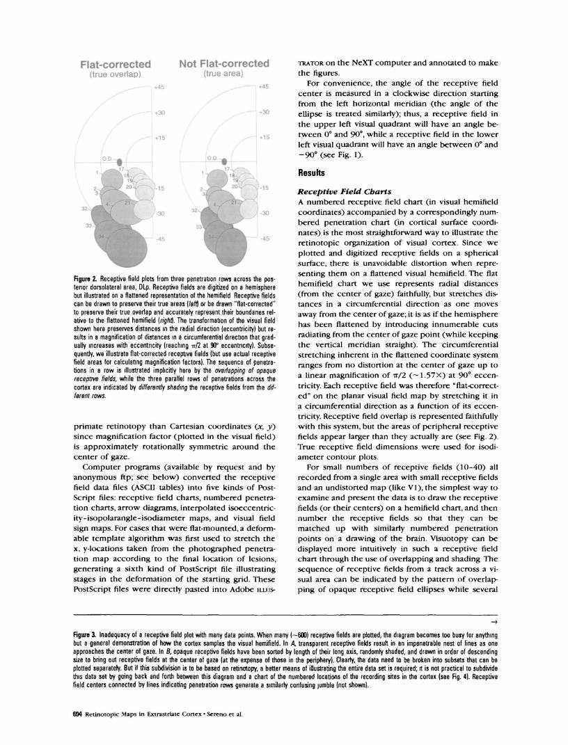
Rgnre 2. Receptive field plots from three penetration rows across the pos-terior dorsolateral area, DLp. Receptive fields are digitized on a hemispherebut illustrated on a flattened representation of the hemifield Receptive fieldscan be drawn to preserve their true areas (/eft) or be drawn "flat-corrected"to preserve their true overlap and accurately represent their boundaries rel-ative to the flattened hemifield (rig/)f). The transformation of the visual fieldshown here preserves distances in the radial direction (eccentricity) but re-sults in a magnification of distances in a circumferential direction that grad-ually increases with eccentricity (reaching u/2 at 90° eccentricity). Subse-quently, we illustrate flat-corrected receptive fields (but use actual receptivefield areas for calculating magnification factors). The sequence of penetra-tions in a row is illustrated implicitly here by the overlapping of opaquereceptive fields, while the three parallel rows of penetrations across thecortex are indicated by differently shading the receptive fields from the dif-ferent rows.

primate retinotopy than Cartesian coordinates (x, y)since magnification factor (plotted in the visual field)is approximately rotationally symmetric around thecenter of gaze.

Computer programs (available by request and byanonymous ftp; see below) converted the receptivefield data files (ASCII tables) into five kinds of Post-Script files: receptive field charts, numbered penetra-tion charts, arrow diagrams, interpolated isoeccentric-ity-isopolarangle-isodiameter maps, and visual fieldsign maps. For cases that were flat-mounted, a deform-able template algorithm was first used to stretch thex, y-locations taken from the photographed penetra-tion map according to the final location of lesions,generating a sixth kind of PostScript file illustratingstages in the deformation of the starting grid. ThesePostScript files were directly pasted into Adobe ILLUS-

TRATOR on the NeXT computer and annotated to makethe figures.

For convenience, the angle of the receptive fieldcenter is measured in a clockwise direction startingfrom the left horizontal meridian (the angle of theellipse is treated similarly); thus, a receptive field inthe upper left visual quadrant will have an angle be-tween 0° and 90°, while a receptive field in the lowerleft visual quadrant will have an angle between 0" and-90° (see Fig. 1).

Results

Receptive Field ChartsA numbered receptive field chart (in visual hemifieldcoordinates) accompanied by a correspondingly num-bered penetration chart (in cortical surface coordi-nates) is the most straightforward way to illustrate theretinotopic organization of visual cortex. Since weplotted and digitized receptive fields on a sphericalsurface, there is unavoidable distortion when repre-senting them on a flattened visual hemifield. The flathemifield chart we use represents radial distances(from the center of gaze) faithfully, but stretches dis-tances in a circumferential direction as one movesaway from the center of gaze; it is as if the hemispherehas been flattened by introducing innumerable cutsradiating from the center of gaze point (while keepingthe vertical meridian straight). The circumferentialstretching inherent in the flattened coordinate systemranges from no distortion at the center of gaze up toa linear magnification of TT/2 (-1.57X) at 90° eccen-tricity. Each receptive field was therefore "flat-correct-ed" on the planar visual field map by stretching it ina circumferential direction as a function of its eccen-tricity. Receptive field overlap is represented faithfullywith this system, but the areas of peripheral receptivefields appear larger than they actually are (see Fig. 2).True receptive field dimensions were used for isodi-ameter contour plots.

For small numbers of receptive fields (10-40) allrecorded from a single area with small receptive fieldsand an undistorted map (like VI), the simplest way toexamine and present the data is to draw the receptivefields (or their centers) on a hemifield chart, and thennumber the receptive fields so that they can bematched up with similarly numbered penetrationpoints on a drawing of the brain. Visuotopy can bedisplayed more intuitively in such a receptive fieldchart through the use of overlapping and shading Thesequence of receptive fields from a track across a vi-sual area can be indicated by the pattern of overlap-ping of opaque receptive field ellipses while several

figure 1 Inadequacy of a receptive field plot with many data points. When many (—600) receptive fields are plotted, the diagram becomes too busy for anythingbut a general demonstration of how the cortex samples the visual hemifield. In A, transparent receptive fields result in an impenetrable nest of lines as oneapproaches the center of gaze. In B, opaque receptive fields have been sorted by length of their long axis, randomly shaded, and drawn in order of descendingsize to bring out receptive fields at the center of gaze (at the expense of those in the periphery). Clearly, the data need to be broken into subsets that can beplotted separately. But if this subdivision is to ba based on retinotopy, a better means of illustrating the entire data set is required; it is not practical to subdividethis data set by going back and forth between this diagram and a chart of the numbered locations of the recording sites in the cortex (see Fig. 4). Receptivefield centers connected by lines indicating penetration rows generate a similarty confusing jumble (not shown).

HM Retinotopic Maps in Extrasuiatc Cortex • Sereno et al.

C e r e b r a l C o n e x N o v / D c c 1 9 9 4 , V 4 N 6 8 B

1 mm

218 * 218219 *»* •

248 248 250 »<247 248 248 2

238 240241 242 S*3 244 • ?*7»W?< * « •

W 3,0 311 31! 3,3 3,4 ,„ , 1 K a

378 3B0 7 ' • 383 a

372 373 374WK * ' " « 378WK « ' « i XJTBNR3U380 set,-, 383 V* &*&t 387 s. . . WE . • • • • .36*° ^ S M S M

4,5 4,7 418 4«*1« ¥«4 , 0 «. 4,2 4,3 4,4 4,5 4,7 V ^ ^ ^ ^ ^

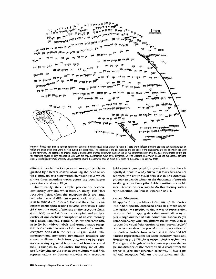
Rgurs 4. Penetration sites in panetal cortex that generated the receptive fields shown in Figure 3. These were digitized from the exposed cortex photograph onwhich the penetration sites were marked during trie experiment The locations of the penetrations and the edge of the craniotomy are also shown in the insetat the lower left The posterior-to-antenor rows of penetrations trended somewhat medially and so the penetration chart and the inset were rotated in this andthe following figures to align penetration rows with the page horizontal to make arrow diagrams easier to interpret The sytvian sulcus and the superior temporalsulcus are marked by thick lines, the loops indicate where the posterior ends of these sulci come to the surface as shallow dents.

different parallel tracks across an area can be distin-guished by different shades, obviating the need to re-fer continually to a penetration chart (see Fig. 2, whichshows three recording tracks across the dorsolateralposterior visual area, DLp).

Unfortunately, these simple procedures becomecompletely unwieldy when there are many (100-600)receptive fields, when the receptive fields are large,and when several different representations of the vi-sual hemifield are involved. Each of these factors in-creases overlapping leading to visual confusion Figure5A shows the result of plotting all the receptive fields(over 600) recorded from the occipital and parietalcortex of one cortical hemisphere of an owl monkeyon a single hemifield. Figure 3B shows the same dataas in 3 4 but without labels, and using opaque recep-tive fields plotted in order of size to make the smallerreceptive fields near the center of gaze visible. Thecorresponding numbered penetration locations areshown in Figure 4. Such busy diagrams can be usefulfor conveying a general impression of how the visualfield is sampled by the cortex, but they are of littleuse for dividing up the cortex into multiple visual fieldrepresentations (a diagram showing only receptive

field centers connected by penetration row lines isequally difficult to read). Given that many areas do notrepresent the entire visual field, it is quite a nontrivialproblem to decide which of the thousands of possiblesmaller groups of receptive fields constitute a sensiblearea There is no easy way to do this starting with arepresentation like that in Figures 3 and 4.

Arrow DiagramsTo approach the problem of dividing up the cortexinto retinotopically organized areas in a more objec-tive fashion, we needed to find a way of representingreceptive field mapping data that would allow us toplot a large number of data points simultaneously, yetcomprehensibly. One straightforward solution is to il-lustrate the visual field location of each receptive fieldcenter as a small arrow placed at the x, y-position onthe cortical surface from which it was recorded (cf.figurine representations for somatosensory maps, andMontero et al., 1973, for a related display technique).The angle and length of each arrow represent the an-gle and distance of the receptive field center from thecenter of gaze (not direction selectivity). Thus, a pe-ripheral receptive field on the horizontal meridian

Rctinotopic Maps ui Extrasiriatc Cortex • Scrcno et al

would be represented as a long horizontal arrowwhile a receptive field on the upper field vertical me-ridian near the center of gaze would be a short up-ward-pointing arrow.

This system is easy to learn and it allows us to plothundreds of receptive fields on one page. It obviateshaving to look back repeatedly at a penetration chart,since the arrow centers themselves are the penetra-tion chart. It is much less time consuming to locatereversals, discontinuities, and visual topography (orlack of it) with this system. Most importantly, it pro-vides a practical way for the reader to verify the de-gree to which the data actually support a particularinterpretation of where the boundaries of visual mapsare located. This system could be adapted to representother kinds of 2D mapping data (e.g., somatosensorymapping data).

Figure 5 shows how two kinds of idealized visualareas appear in an arrow diagram. On the left is amirror-image representation of the visual field (likeVI); this appears in an arrow diagram as a pure shearfield. On the right is a non-mirror-image representation(like V2, but without a split horizontal meridian). This,by contrast, appears as a pure contraction field. Theseidealized areas were arranged so that their vertical andhorizontal meridians were aligned with the page. Theupper visual field arrows are drawn with a thicker linethan the lower visual field arrows to highlight the up-per/lower field distinction.

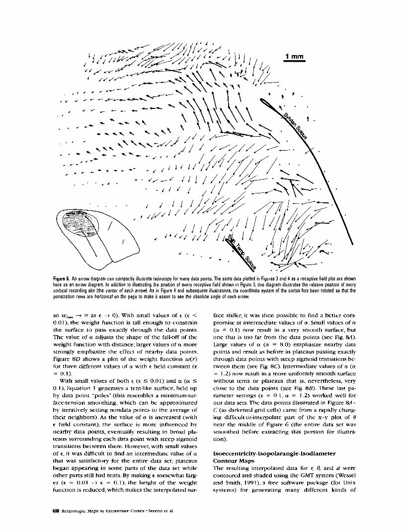
Figure 6 is an arrow diagram of all the data fromthe very dense receptive field chart in Figure 3. It isnow much easier to see systematic changes in recep-tive field location as electrode penetration sequencespass through multiple visual areas in parietal cortex.Since oblique rows of arrows generate an orientationsurround effect that makes it difficult to see true hor-izontal or true vertical (relative to the page bound-aries) for an individual arrow, the coordinate systemof the cortex for each case was rotated until penetra-tion rows were oriented approximately horizontally.

For areas sampled by penetration rows orientedperpendicular to their vertical meridians, it is straight-forward to rotate the cortical coordinate system sothat the vertical meridian is vertical on the page andmirror-image and non-mirror-image representationsappear as they do in the idealized areas in Figure 5.With a more extensive map, it becomes impossible todo this simultaneously for all areas. As the vertical me-ridian of an area assumes different angles with respectto the page (but the individual arrows continue to bedrawn with respect to the page horizontal and pagevertical to guarantee their context-free interpretabili-ty) arrow fields for both mirror-image and non-mirror-image areas will acquire rotational components (seeFig. 7). Non-mirror-image regions can still be distin-guished from mirror-image regions because onlymirror-image regions contain shear components (for-malized below). This is a subtle visual difference,however, and so we decided to make explicit maps ofvisual field sign.

Left Visual Field/Right Hemisphere

mirror-imagearea (e.g., V1)

/ / /

S / /

\ \ \\ \ \ \

t

K non-mirror imagearea (e.g., V2)

/ / / /

\ \ \ V\ \ \ \

Figure 5. How mirror-image and non-mirror-image areas appear in an arrowdiagram. On the /eft, a mirror-image representation of the left visual field (likeright hemisphere VI) is illustrated. It appears as a shear field (arrows tangentto y = rrvr'). On the right a non-mirror-image representation is illustrated(like V2, but without a split horizontal meridian). It appears, by contrast as asimple contraction field {arrows along y = mx).

Interpolating Sparse Data onto aRegular x-y GridAn arrow diagram faithfully illustrates the discrete andsomewhat noisy nature of the mapping data. However,there is also a need for maps interpolated onto a uni-form grid. These can then be contoured and used toestimate local visual field sign (see below). Since thereare two main coordinates of retinotopy at each pointin the cortex (eccentricity, r, and angle, 0)> we needto superimpose two contour plots to illustrate retin-otopy. A third coordinate is the receptive field diam-eter, d, which can be used to estimate the degree towhich a particular region of the cortex smears an im-age. We used a distance-weighted smoothing methodto interpolate the scattered r, 0, and d data onto uni-form x-y grids (Lancaster and Salkauskas, 1986; Zipserand Andersen, 1988). The interpolated value £y at theyth grid point was the distance-weighted sum of thevalues, z,, of all of the surrounding YV data points,scaled by the sum of the weights:

where the weight for the /th data point, uKr^), was anexponential function of the distance rtJ (in mm) be-tween the ixh data point and theyth grid point:

uKr) = e-^/Cr2 + e) (2)The weight function has a maximum at r = 0, that is,when a grid point lies exactly on a data point. Thismaximum height is set by the value of e (w^, = e~'

Cerebral Cortex Nov/Dec 1994, V 4 N 6 607

w vrr 1 mm

\\\vv: -

Figure 6. An arrow diagram can compactly illustrate retinotopy for many data points. The same data plotted in Figures 3 and 4 as a receptive field plot are shownhere as an arrow diagram. In addition to illustrating the position of every receptive field shown in Rgure 3, this diagram illustrates the relabve position of everycortical recording site (the center of each anoWi. As in figure 4 and subsequent illustratons, the coordinate system of the cortex has been rotated so that thepenetration rows are horizontal on the page to make it easier to see the absolute angle of each arrow.

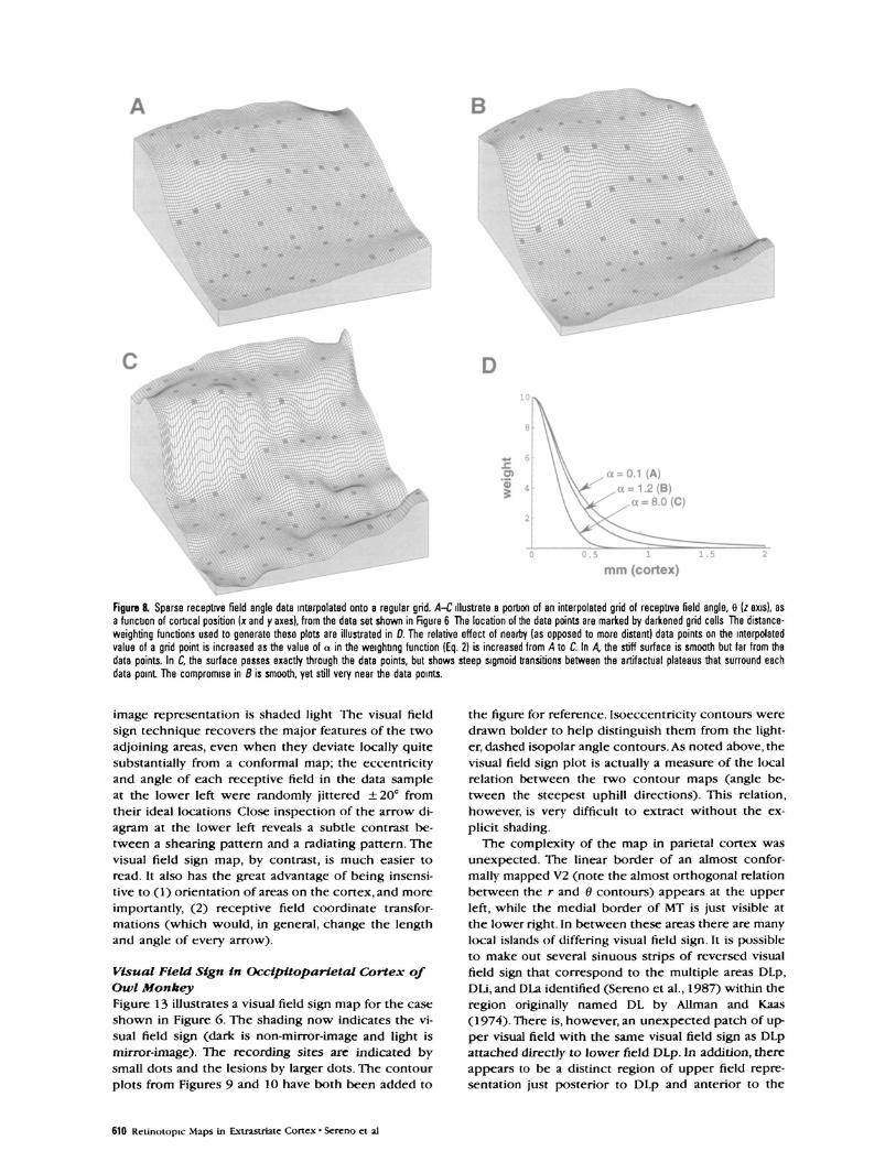
so w^ —» oo as e —> 0). With small values of e (e <0.01), the weight function is tall enough to constrainthe surface to pass exactly through the data points.The value of a adjusts the shape of the fall-off of theweight function with distance; larger values of a morestrongly emphasize the effect of nearby data points.Figure 8D shows a plot of the weight function w{f)for three different values of a with e held constant (e= 0.1).

With small values of both e (e £ 0.01) and a (a =£0.1), Equation 1 generates a tent-like surface, held upby data point "poles" (this resembles a minimum-sur-face-tension smoothing, which can be approximatedby iteratively setting nondata points to the average oftheir neighbors). As the value of a is increased (withe held constant), the surface is more influenced bynearby data points, eventually resulting in broad pla-teaus surrounding each data point with steep sigmoidtransitions between them. However, with small valuesof e, it was difficult to find an intermediate value of athat was satisfactory for the entire data set; plateausbegan appearing in some parts of the data set whileother parts still had tents. By making e somewhat larg-er (e = 0.01 —> e = 0.1), the height of the weightfunction is reduced, which makes the interpolated sur-

face stiffer; it was then possible to find a better com-promise at intermediate values of a. Small values of a(a = 0.1) now result in a very smooth surface, butone that is too far from the data points (see Fig. &4).Large values of a (a = 8.0) emphasize nearby datapoints and result as before in plateaus passing exactlythrough data points with steep sigmoid transitions be-tween them (see Fig. 8C). Intermediate values of a (a= 1.2) now result in a more uniformly smooth surfacewithout tents or plateaus that is, nevertheless, veryclose to the data points (see Fig. 85). These last pa-rameter settings (e = 0 1, a = 1.2) worked well forour data sets.The data points illustrated in Figure 8A-C (as darkened grid cells) came from a rapidly chang-ing difficult-to-interpolate part of the x-y plot of dnear the middle of Figure 6 (the entire data set wassmoothed before extracting this portion for illustra-tion).

Isoeccentriclty-Isopolarangle-IsodlameterContour MapsThe resulting interpolated data for r, d, and d werecontoured and shaded using the GMT system (Wesseland Smith, 1991), a free software package (for Unixsystems) for generating many different kinds of

SB Retlnotopic Maps In Extrastriatc Cortex • Screno el al

PostScript output maps from ASCII tables (available byanonymous ftp from kaiwe.soest.hawaii.edu). TheGMT system software was also used to generate thesurface plots of our interpolated data in Figure 8A-C

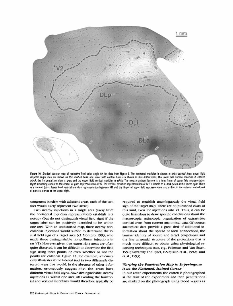
Figure 9 shows a shaded contour map of r for thecase shown in Figure 6. In this plot, the center of gaze(small eccentricity) is dark and the periphery is light.There is a general tendency in parietal cortex for ec-centricity to increase as one moves rostrally, althoughthere are several pockets of small eccentricity rostrally.Figure 10 shows a shaded contour map of 8, also forthe case from Figure 6, where the lower field verticalmeridian (—90°) is dark, the horizontal meridian (0°)is gray, and the upper field vertical meridian (+90°) islight. The picture of 0 is quite complex; there are anumber of representations of the horizontal meridian(marked by thick dashed lines) as well as the upperand lower field vertical meridians.

A map of cortical retinotopy would be obtained bysuperimposing the two maps from Figures 9 and 10.When the data set contains multiple, distorted repre-sentations, however, it can be exceedingly difficult toread such a map. There are two superimposed sets ofcontours, each with its own labels, and there is noeasy way to shade both of them at the same time (tohelp indicate the direction in which each set of con-tours is increasing). The fundamental problem with adouble contour plot is that individual re-representa-tions of the visual field do not stand out in any way.Boundaries between visual areas appear on doublecontour plots only as a change in the angle at whichthe r and 8 contours intersect. The difficulty in read-ing these maps prompted us to look for a better wayof representing the data. We turned to a map shadedby local visual field sign (non-mirror-image vs mirror-image); the double contour map was retained under-neath for reference.

Visual Field Sign MapsFor each small portion of a retinotopic cortical map,one can calculate the sign of the visual field represen-tation—that is, whether it is a non-mirror-image ormirror-image representation of the retina (whenviewed from the cortical surface). The visual field signcan be determined from the (clockwise) angle, A, be-tween the direction of the gradient in eccentricity, Vr,and the direction of the gradient in angle, V0 (see Fig.11) (the gradients are locally perpendicular to thecontour lines and point uphill). An angle between thegradient directions of IT/2 signifies an undistorted(conformal) non-mirror-image representation while anangle of 3TT/2 signifies an undistorted mirror-imagerepresentation. Intermediate angles signify differentdegrees of nonorthogonality (nonconformality) of thevisual field representation with singularities at 0 andIT, where visual field regions would be mapped tolines of indeterminate visual field sign. A map of visualfield sign is produced by distinguishing A between 0and TT from \ between TT and 2TT. The local gradientdirections in the r and 8 maps are estimated from fi-nite differences in the x- and y-directions on the twointerpolated maps.

/ / / iI / / / /I / / / /

• \ \ vvt \ \ \ NM\\\

\ \\ \\ \t\ \\ \w\ \

\•

\

• ' / /

• / /

- - - • / /- - - • • /

Figure 7. Difficulty of extracting visual field sign from an arrow diagramWhen the vertical mendian of a cortical visual area is not onented verticallyon the page, rotational components are added to both non-mirror-image andmirror-image representations (since the arrows are always drawn relative tothe page coordinate system to guarantee their context free interpretabilfty)Since vertical meridians of real cortical areas are often not parallel to eachother, and since penetration rows are often not orthogonal to vertical merid-ians, it can be quite difficult to distinguish these two kinds of maps.

Visual field sign has several attractive properties asa local measure of cortical organization. First, since itis a relative measure, it is invariant to the orientationof the retinotopic map on the cortex (see Fig. 11).Second, and somewhat less obviously, visual field signis invariant to rigid transformations of the receptivefield coordinate system (as would be produced, e.g.,by sliding and/or rotating a sheet of spherical papercontaining receptive fields over the surface of theplastic hemisphere coordinate system). This is againbecause of the fact that visual field sign is a relativemeasure; the r and 8 gradient directions are bothchanged in the same way by such a transformation.Thus, the analysis is completely insensitive to theplacement of the center of gaze, the vertical meridian,and so on. The only requirement is that the receptivefields all be digitized using the same (arbitrary) coor-dinate system.

Figure 12 (top row) illustrates the technique ap-plied to an idealized pair of adjoining visual areas (likethose shown in Fig. 5) and a more realistic, randomlyjittered pair of areas sampled at a density typical ofour experiments (bottom row). In both rows, the start-ing data are shown in the arrow diagrams at the farleft. Eccentricity, r, and angle, 8, of each of these datasets were then interpolated onto regular grids usingthe distance-weighting function used in Figure SB.The resulting r and 8 grids were contoured and shad-ed in the middle two panels (top and bottom rows)The r and 8 grids were then combined to make visualfield sign maps at the far right (the two contour plotsare also superimposed for reference), where non-mir-ror-image representation is shaded dark and mirror-

Cerebral Cortex Nov/Dec 1994, V 4 N 6 609

a = 0.1 (A)a = 1.2 (B)

a = 8.0 (C)

0 . 5 1

mm (cortex)1.5

Figure 8. Sparse receptive field angle data interpolated onto a regular grid. A-C illustrate a portion of an interpolated grid of receptive field angle, 8 (z axis), asa function of cortical position (x and y axes), from the data set shown in Rgure 6 The location of the data points are marked by darkened grid cells The distance-weighting functions used to generate these plots are illustrated in D. The relative effect of nearby (as opposed to more distant) data points on the interpolatedvalue of a grid point is increased as the value of a in the weighting function (Eq. 2) is increased from A to C. In A the stiff surface is smooth but far from thedata points. In C, the surface passes exactly through the data points, but shows steep sigmoid transitions between the artifactual plateaus that surround eachdata point The compromise in 8 is smooth, yet still very near the data points.

image representation is shaded light The visual fieldsign technique recovers the major features of the twoadjoining areas, even when they deviate locally quitesubstantially from a conformal map; the eccentricityand angle of each receptive field in the data sampleat the lower left were randomly jittered ±20° fromtheir ideal locations Close inspection of the arrow di-agram at the lower left reveals a subtle contrast be-tween a shearing pattern and a radiating pattern. Thevisual field sign map, by contrast, is much easier toread. It also has the great advantage of being insensi-tive to (1) orientation of areas on the cortex, and moreimportantly, (2) receptive field coordinate transfor-mations (which would, in general, change the lengthand angle of every arrow).

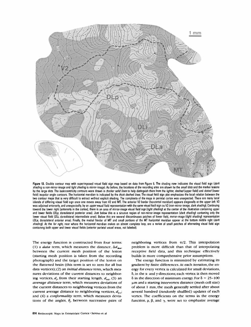
Visual Field Sign in Occipitoparietal Cortex ofOwl MonkeyFigure 13 illustrates a visual field sign map for the caseshown in Figure 6. The shading now indicates the vi-sual field sign (dark is non-mirror-image and light ismirror-image). The recording sites are indicated bysmall dots and the lesions by larger dots. The contourplots from Figures 9 and 10 have both been added to

the figure for reference. Isoeccentricity contours weredrawn bolder to help distinguish them from the light-er, dashed isopolar angle contours. As noted above, thevisual field sign plot is actually a measure of the localrelation between the two contour maps (angle be-tween the steepest uphill directions). This relation,however, is very difficult to extract without the ex-plicit shading.

The complexity of the map in parietal cortex wasunexpected. The linear border of an almost confor-mally mapped V2 (note the almost orthogonal relationbetween the r and d contours) appears at the upperleft, while the medial border of MT is just visible atthe lower right. In between these areas there are manylocal islands of differing visual field sign. It is possibleto make out several sinuous strips of reversed visualfield sign that correspond to the multiple areas DLp,DLi, and DLa identified (Sereno et al., 1987) within theregion originally named DL by Allman and Kaas(1974). There is, however, an unexpected patch of up-per visual field with the same visual field sign as DLpattached direct!)' to lower field DLp. In addition, thereappears to be a distinct region of upper field repre-sentation just posterior to DLp and anterior to the

610 Rctinotopic Maps in Extrastriate Cortex • Scrcno et al

1 mm

Figure 9. Shaded contour map of interpolated receptive field eccentricity {r) for data from Rgure 6. Central to peripheral visual fields are shaded dark to lightThere is an overall tendency for eccentricity to increase as one moves both medially and anteriorly in occipitoparietal cortex. However, there are several pocketsof center of gaze representations at the anterior and medial extremes of panetal cortex. The locations of the recording sites are shown by the small dots andthe marker lesions by the large dots

lower visual field representation in V2 with the samevisual field sign as V2. There are also several smallareas directly medial to MT. The complexity of thepicture is at odds with the usual summary diagrams(this case will be discussed in detail in a subsequentarticle).

We tested the effects of changing the distance-weighted smoothing coefficients, e and a, on the vi-sual field sign map shown in Figure 13. The overallpattern of visual field sign and also the position of thevisual field sign transitions were quite stable tochanges in these parameters, breaking down onlywhen the interpolated surfaces were extremely stiff(smooth), excessively tented, or strongly locally influ-enced (plateaus with sigmoid transitions). With overlystiff interpolations, smaller pockets of reversed visualfield sign were lost. With excessively tented smooth-ings, artifactual visual field sign reversals appearedaround the tents at each data point. With strongly lo-cally influenced smoothings, visual field sign bound-aries were artifactually squared up because penetra-tions were sometimes made in rows. These smoothing

artifacts were virtually eliminated with appropriatechoices of e and a.

Difficulty of Obtaining Visual Field Sign fromConnectional DataIt should be noted that it is very difficult to obtainvisual field sign maps from corticocortical connectionaldata when visual areas (1) are small, (2) are variable,(3) have distorted representations of the retina, (4)have borders that are not architectonically apparent,and (5) have split horizontal meridian representations.These, unfortunately, are characteristics of most visualareas beyond VI. A single injection only establishes thatthere are connections between areas. If the injection isnear an areal border, a single labeled focus may actuallyrepresent two labeled areas joined by a congruent bor-der. There are additional complications if the injectionencroaches on a horizontal meridian representationsince this may result in two foci appearing in a singletarget area if the target area's horizontal meridian issplit (actually, since horizontal meridians often form

CcrebraJ Cortex Nov/Dcc 1994, V 4 N 6 611

1 mm

MT..rvJ.Figure 10. Shaded contour map of receptive field polar angle (0) for data from Figure 6. The horizontal meridian is shown in thick dashed lines, upper fieldisopolar angle lines are shown as thin dashed lines, and lower field contour lines are shown as thin dotted lines. The lower field vertical meridian is shadedblack, the horizontal meridian is gray, and the upper field vertical meridian is white. The most prominent feature is a long finger of upper field representation{lighfi extending almost to the center of gaze representation of V2. The vertical meridian representation of MT is visible as a dark patch at the lower right Thereis a second (dark) lower field vertical meridian representation between MT and the finger of upper field representation, and a third in the anterior medial partof parietal cortex at the upper right

congruent borders with adjacent areas, each of the twofoci would likely represent two areas).

Two nearby injections in a single area (away fromthe horizontaJ meridian representation) establish reti-notopy (but do not distinguish visual field sign) if thetarget label can be positively identified to be withinone area. With an undistorted map, three nearby non-collinear injections would suffice to determine the vi-sual field sign of a target area (cf. Montero, 1993, whomade three distinguishable noncollinear injections inrat VI). However, given that extrastriate areas are oftenquite distorted, it can be difficult to determine the fieldsign using three points, or even whether or not thepoints are collinear. Figure 14, for example, schemati-cally illustrates three labeled foci in two differently dis-torted areas that would, in the absence of other infor-mation, erroneously suggest that the areas havedifferent visual field signs. Four distinguishable, nearbyinjections all within one area, all avoiding the horizon-tal and vertical meridians, would therefore typically be

required to establish unambiguously the visual fieldsign of the target map. There are no published cases ofthis kind, even for injections into VI. Thus, it can bequite hazardous to draw specific conclusions about themacroscopic retinotopic organization of extrastriatecortical areas from current anatomical data. Of course,anatomical data provide a great deal of additional in-formation about the spread of local connections, thelaminar identity of source and target projections, andthe fine tangential structure of the projections that ismuch more difficult to obtain using physiological re-cording techniques (see, e.g., Felleman and Van Essen,1991; Kisvarday and Eysel, 1992;Salin et al., 1992; Lundet al., 1993).

Warping tbe Penetration Map to SuperimposeIt on tbe Flattened, Stained CortexIn our acute experiments, the cortex is photographedat the start of the experiment and then penetrationsare marked on the photograph using blood vessels as

612 Retinotopic Maps In Extrastriate Cortex • Sereno et al.

Non-mirror-imageleft hemifield map

( A 7 1 / 2 )

Mirror-imageleft hemifield map

(k = 3n/2)

Figure 11. The local visual field sign is determined by measuring the (clock-wise) angle, A, between the eccentricity gradient (direction of Vf), and thereceptive field polar angle gradient (direction of V0). An angle of approxi-mately 90° (0 < A < n) signifies a non-minor-image mapping of the contra-lateral (left) hemifield while an angle of approximately 270° |TT < X < 2 IT)signifies a mirror-image mapping of the same hemifield. This is a robustrelative local measure capable of distinguishing non-mirror-image from mir-ror-image regions that is invariant to rotation and distortion of local mapregions. Visual field sign is also invariant to receptive field coordinate trans-formations; to compute it, only the relative position of receptive fields mustbe known.

landmarks, as described above. The x, y-locations ofthe penetrations are digitized from the photographand can be used to make arrow diagrams, isoeccen-tricity/isopolar angle maps, and visual field sign maps.The resulting maps, however, must then be related tothe stained, flattened cortex using marker lesions. Ifthe flattening process only involved global scaling (ex-pansion/contraction) and rotation, it would be a sim-ple matter to superimpose the photograph-derivedpenetration maps on the stained cortex. The physicalflattening process, however, involves local expansions,rotations, and shears. Therefore, we devised a deform-able template technique to stretch the x-y photo-graphic penetration map according to final location oflesion control points in the stained tissue.

The technique works by establishing a mesh withsquare cells and then moving each of the vertices ofthe mesh so as to minimize a local energy function,Er The value of E for the fth vertex is calculated frommarker lesion errors and from distances to, and anglesbetween, the neighboring N vertices (yV = 4 exceptfor corner and edge points):

+ 6 -

+ p

|

N

K

X

y* \d -- d

(3)

/ / / // / / /

/ I I; i i/ i i

/ / / // // /

V \ \ \ \ t \ \ \ \ N

i. 1 I

N ^ V 'v \

\

fe

Hgare 12. Regular and jittered hemifield maps anaLzed by arrow diagrams, contour plots, and visual field sign maps. The top row snows a square cortical patchcontaining two visual areas sharing a vertical meridian analyzed by four different techniques: from left to right, an arrow diagram, a shaded contour plot ofreceptive field eccentricity [r], a shaded contour plot of receptive field polar angle (d), and finally a map of visual field sign (the gray border indicates the finiteinterval over which the gradients used to calculate field sign were estimated). The bottom row shows these four techniques applied to a jittered, more sparselysampled version of the two areas; this closely approximates the sampling density and rate of change of receptive field coordinates in real data. The interpolationand visual field sign analysis recovers the basic form of the two areas at the bottom far right, despite the fact that the eccentricity and angle of each receptivefield have been jittered substantially from their idealized positions. The jittered data set was constructed by starting with a grid of randomly jittered x, y-locations,calculating the ideal receptive field position for each of these x, y-positions using an MT-like expansion of the center of gaze, and then randomly jittering theeccentricity and angle of the receptive field centers (using random numbers drawn from a flat distribution of ±20°). The visual field sign map at the lower rightis much easier to read than the equivalent arrow diagram at the lower left, where field sign is indicated only by a much more subtle distinction between shearingand contracting vector fields.

Cerebral Cortex Nov/Dcc 1994, V 4 N 6 613

1 mm

Figure 13. Double contour map with superimposed visual field sign map based on data from Figure 6. The shading now indicates the visual field sign {darkshading is non-mirror-image and light shading is mirror-image). As before, the locations of the recording sites are shown by the small dots and the marker lesionsby the large dots. The isoeccentricity contours were drawn in thicker solid lines to help distinguish them from the lighter, dashed (upper field) and dotted (lowerfield) isopolar angle contours. The horizontal meridian is indicated by the thick dashed lines. The visual field sign plot emphasizes the local relation between thetwo contour maps that is very difficult to extract without explicit shading. The complexity of the maps in parietal cortex was unexpected. There are many localislands of differing visual field sign once one moves away from V2 and MT. The anterior V2 border (horizontal meridian) appears diagonally at the uppar left V2was adjoined antenorty, and unexpectedly, by an upper visual field representation with the same visual field sign as V2 (non-mirror-image, dark shading). Continuingtoward the lower right (antenorty in the cortex), there is an area of mirror-image visual field sign {light shading) at the center of the illustration containing upperand lower fields {Dip, dorsolateral posterior area). Just below this is a sinuous region of non-mirror-image representation {dark shading) containing only thelower visual field {DLi, dorsolateral intermediate area). Below this are several discontinuous patches of lower field, mirror-image [light shading) representation{DLa, dorsolateral anterior area). Finally, the medial border of MT and small portions of the MT horizontal meridian appear at the bottom middle right {darkshading). At the far right, near where the horizontal meridian makes an almost complete loop, are a series of small patches of alternating visual field signcontaining both upper and lower visual fields (anterior parietal visual areas, not labeled).

The energy function is constructed from four terms:(1) a data term, which measures the distance, Arf^,between the current mesh position of the lesion(starting mesh position is taken from the recordingphotograph) and the target position of the lesion onthe flattened brain (this term is set to zero for all butdata vertices); (2) an initial distance term, which mea-sures deviations of the current distances to neighbor-ing vertices, dj, from their starting length, djM, (3) anaverage distance term, which measures deviations ofthe current distances to neighboring vertices from thecurrent average distance to neighboring vertices, d^c;and (4) a conformality term, which measures devia-tions of the angles, 6p between successive pairs of

neighboring vertices from n/2. This interpolationproblem is more difficult than that of interpolatingreceptive field data, and this technique effectivelybuilds in more comprehensive prior assumptions.

The energy function is minimized by estimating itsgradient by finite differences. At each iteration, the en-ergy for ever)r vertex is calculated for small deviations,8, in the x- and y-directions; each vertex is then moved8 in the direction of minimum energy. For 8 = 25-100jim and a starting intervertex distance (mesh cell size)of about 1 mm, the mesh generally settled after aboutseveral hundred (randomly shuffled) updates of eachvertex. The coefficients on the terms in the energyfunction, p, £, and -y, were set to emphasize average

614 Rctinotoplc Maps In Extrastriatc Cortex - Scrcno « 2|

distance and orthogonality over initial distance. Thisgenerates mesh deformations that closely resemblethe deformations observed in the physical flatteningprocess as the cortical tissue is lightly compressed be-tween slides prior to fixation. To speed convergence,we included a momentum term (which incorporatesa portion of the previous move into the currentmove). As the mesh settles, the first-order data termdominates, forcing the lesions to lie exactly at theirflattened brain positions, which simplifies the finaloverlay. The final locations of the penetration pointsare calculated by bilinear interpolation using the finallocation of the four mesh vertices that were nearesteach penetration point in the undeformed mesh.

A deformed mesh calculated using eight identifiedlesion points is illustrated in Figure 15. The stretchingprocess is illustrated by drawing the final mesh on alarge rectangle, which illustrates the initial borders ofthe mesh, and by drawing a line between the initiallocation of each of the —600 penetrations (small opendots) and their final, stretched location (small soliddots). The initial and starting positions of the lesionsare indicated by medium-sized open and solid dots,and lines. Finally, the initial and target locations of themesh points nearest the lesions (which are used tocalculate the data term) are shown as large, and slight-ly larger open circles. The stretched x, y-locationswere used to make the isoeccentricity, isopolar anglemaps, and visual field sign maps so that they could beaccurately superimposed on stained flat-mounts. Thefinal mesh appears deceptively undistorted. Close in-spection of the starting and ending positions of thelesions and recording sites, however, reveals a com-plex pattern of local movement across the cortex thatwould be poorly approximated by global scaling, ro-tation, and shear. Our technique also works in in-stances where flattening-induced deformations aremore severe and more anisotropic.

DiscussionMultiple retinotopic maps characterize the tangentialorganization of most of the visual half of neocortex inprimates. Physiological mapping experiments are acrucial tool for defining visual areas. No other tech-nique offers as detailed a window on the organizationof extrastriate cortex in single animals. The ability toexamine the organization of visual areas within a sin-gle animal is particularly important given the largeamount of variability that exists between animals ofthe same species.

In the course of collecting and attempting to ana-lyze large retinotopic mapping data sets from owlmonkey extrastriate cortex, it became quite clear thatcurrent methods for representing this kind of datawere inadequate. In this article, we have presentedseveral analytic techniques—arrow diagrams and vi-sual field sign maps—that make it possible to parcelvisual cortex more objectively into different areas onthe basis of retinotopy. These techniques could be ex-tended to other modalities characterized by 2D recep-totopic maps (e.g., somatosensory cortex). We post-pone detailed discussion of the individual areas

Visual Raidretinotopic locationof three injections

Cortical Areasspurious indication of

opposite visual field sign

figure 14. Difficulty of determining visual field sign with tracer injectionsalone. The visual field locations of three distinguishable tracer inactions areillustrated at the left The label in two differently distorted cortical areas withthe same visual field sign are shown at the right In the absence of otherinformation, a plot of the distribution of the three tracers would spuriouslysuggest that the two areas have opposite visual field sign (i.e., the triangleformed by injections 1, 2, and 3 is reversed in the two areas). Differentlydistorted areas, of course, would cause similar problems with injections clos-er to isoeccentricrty lines. For injections with realistic separations, one there-fore typically requires four, mutually distinguishable injections, all avoidingthe vertical and horizontal meridians, to determine the visual field sign of anarea anatomically.

revealed in the case illustrated in detail here to ourtwo forthcoming companion articles.

Definition of a Visual AreaMost recent reviews of the organization of visual areas(e.g., Felleman and Van Essen, 1991; Kaas and Krubitz-er, 1991; Sereno and Allman, 1991) illustrate all arealboundaries as uniform dark lines. Though this makesthe maps easier to read, it has a strong tendency todownplay the substantial differences in the degree towhich the various boundaries are supported by con-verging data from retinotopic organization, architec-tonic features, connections patterns, and physiologicalproperties. Some visual areas have boundaries that arewell defined and concordant for all of these criteria.For example, primary visual cortex, area VI, in pri-mates (and other mammals) contains a fine-grained,relatively undistorted map of the entire contralateralvisual hemifield. The electrophysiologically definedborders of this map coincide exactly with a very cleararchitectonic and connection-defined border.

Most of the 25 or so other visual areas are not aseasy to delimit. There are complications even with ar-eas V2 and MT. V2 seems to contain three intercalatedrepresentations of the hemifield in at least the thick,thin, and interstripes (Rosa et al., 1988; Van Essen etal., 1990). In MT, there is a sudden reduction in mye-lination in the representation of the visual field pe-riphery in both owl monkeys and macaque monkeysthat does not seem to have electrophysiological or ret-inotopic correlates (e.g., visual field re-representa-tions) (Allman and Kaas, 1971; Gattass and Gross,1981; Desimone and Ungerleider, 1986). Despite thesedifficulties, however, there is good agreement betweendifferent methods on the location of substantial por-tions of the borders of V2 and MT.

Unfortunately, it is much more difficult to defineunambiguously the borders of most of the visual areasbeyond V2 and MT in extrastriate cortex. There are a

CcrebraJ Cortex Nov/Dcc 1994, V 4 N 6 615

__ —

wI 1

—c^-

—

i

U_ m

M

9 «

a

i» <

t '

„ —

*

» i

J

8

» *

<*

8

8

*

8

» •

. •

1 99

" * *

<* *

8 <

8

8

» •

-

,# *

! 8

9

a i

„„ ,

$ s8<

#

Gi (

a * a

/ ^ /

i«t a*

* c

c»

m

• •

<• a

•crV

*

* c

(f I

If

0* 0

* * 0

. -

<f

if c

,» «

^ c

CM

-

or

*

• 0

a.

- •

•

itfr t 44"r°~* 1t"

r ) | | f [" f / | |

a*

• a

T **l / 1

• o .

1

{—m

<

• #

1 (^

CM

t **°*

»|1 °*

HJ

«. kL 4 0,

<m•1?—

rr t

•*

t in

**

! 8 S j88

s

—v

9

•

r1

Figure 15. Deformed mesh calculated using eight identified lesion points (data from Rg. 6). The large rectangle illustrates the initial borders of the mesh. Thm

lines are drawn between the initial location of each of the —600 penetrations (small open dots] and the final, stretched location (5ms// solid dots). The initial andstarting positions of the marker lesions are indicated by medium-sized open and solid dots, and lines. Rnally, the initial and target locations of the mesh points

nearest the lesions (which are what are actually used to calculate the data term) are shown as large, and slightly larger open circles, and lines. Close examinationof the starting and final penetration pairs in different parts of the diagram reveals a complex pattern of local distortion that cannot be closely approximated byglobal rotation and scaling.

number of reasons for this. First, the architectonic bor-ders of these areas are generally much less distinctthan those of VI, V2, and MT. Second, these areas oftencontain only partial maps of the visual hemifield oreven partial maps of one visual quadrant. Third, themaps are more distorted than those in VI and MT.Fourth, responses in these other areas are often moreleisurely and more susceptible to anesthetic than re-sponses in VI, V2, and MT. Fifth, receptive fields aregenerally larger, and therefore take longer to map. Fi-nally, the areas themselves are often smaller. Theseconsiderations demand a rigorous approach.

Quantitative Retinotopic MapsDouble contour maps have often been presented inanalyses of retinotopy (Allman and Kaas, 1971; Wagoret al., 1980; Desimone and Ungerleider, 1986; Fiorani etal., 1989; Rosa et al., 1993) Yet these have rarely beenexplicit!)' derived by quantitatively interpolating andcontouring the data from an individual case. For ex-

ample, the extensive mapping studies of Tusa, Palmer,and Rosenquist (Tusa et al., 1978, 1979; Palmer et al.,1978; Tusa and Palmer, 1980) present a considerableamount of the raw mapping data (electrode penetra-tion tracks illustrated on sections with correspondinglynumbered receptive field charts) along with summarydouble contour maps. It would be interesting to seequantitatively interpolated, double contour maps for in-dividual cases showing the location of the data points.To be sure, generating quantitative contour maps ismore difficult in cats (and macaque monkeys) than inowl monkeys because of the extensive gyrification ofdie cortex. A more rigorous approach would have tobegin with a computational flattening of die cortex (see,e.g., Schwartz, 1990; Dale and Sereno, 1993) prior tointerpolating and contouring the receptive field data.In another set of extensive studies of retinotopy in pri-mate extrastxiate cortex, sometimes only one coordi-nate of retinotopy (eccentricity) was contoured (Gat-tass et al., 1988; Rosa et al., 1988).

616 Retinotopic Maps in Ertrastriatc Cortex • Sereno et al.

The noniterative distance-weighted interpolation/smoothing technique presented here provides a ro-bust and straightforward way to interpolate sparse ret-inotopic mapping data onto a regular x-y grid oncethe cortex has been flattened. These grids (of r and(?) can then be quantitatively contoured. Existing datafrom areas with obvious architectonic borders suggestthat extrastriate areas vary considerably in size, shape,and location. The cytochrome oxidase-stained flat-mounts illustrated by Tootell et al. (1985), for example,show that the surface area of area MT probably variesby almost a factor of 2 in animals with similar bodysizes. Rigorous interpolation and contouring of map-ping data are a crucial step in better understandinghow the remaining majority of visual areas with muchless well-defined architectonic borders are organized.

Maunsell and Van Essen (1987) presented a quan-titative technique for interpolating sparse receptivefield data from a single area (MT) onto a regular grid.Each grid cell for r (or #) was set to the average ofthe linearly interpolated r (or 0) value along lines be-tween all pairs of data points up to 3 mm apart thatpassed through that grid cell. Their technique (withlines :£ 3 mm) produces a much stiffer surface glob-ally' than our distance-weighted technique does (withe = 0.1, a = 1.2) since it effectively gives equal weightto points that lie within a 6 mm circle (see Fig. 8).However, since it smooths much more over local ret-inotopic details such as minima and maxima in r and8, which are often important for defining areal bound-aries, it is less suited to interpolating data sets con-taining several small visual areas. In addition, thoughglobally stiffer, the Maunsell and Van Essen techniqueproduces surfaces that are locally much less smooth(since a point contributing to one grid cell may oftennot contribute to the neighboring grid cell); these dis-continuities (which are exacerbated by reducing themaximum line length) lead to artifacts when there isa need to estimate derivatives (gradients).

Better Representations of RetinotopyOur large data sets made it necessary to find moreintuitive methods for representing retinotopy. In par-ticular, the standard technique of numbered receptivefield plots with correspondingly numbered penetra-tion charts proved to be completely unwieldy. Recep-tive field plots are useful once the data have beendivided into areas, but we needed to find another wayof representing the data prior to dividing it up. Thenumber of possible subdivisions becomes very largewhen there are several hundred recording sites.

We presented two complementary techniques—ar-row diagrams and visual field sign maps—that makeit easier to parse cortical retinotopic maps visually. Ar-row diagrams are made by placing a small arrowwhose length and angle represent the location of thereceptive field center at the cortical x, y-location ofthe site from which it was recorded. With this tech-nique, it is possible to look at all of the raw data fromone animal at once. This makes it much easier to lookfor receptive field reversals, and to examine the de-gree to which retinotopy is systematic. It is also pos-

sible to distinguish whether an area has a non-mirror-image representation of the hemifield (like V2) or amirror-image representation (like VI); non-mirror-im-age regions have a radiating pattern while mirror-im-age regions have a shearing pattern (see Fig. 5). Re-versals are much easier to mark on an arrow diagramthan on a penetration chart because one does nothave to look up numbers on a crowded receptive fieldchart. Once areal boundaries have been marked, it isa much simpler task for the reader to verify the extentto which the data support a particular subdivision ofthe cortex.

One problem with arrow diagrams is that re-repre-sentations of parts of the visual field sometimes donot stand out clearly. Systematic changes in arrow di-rection (receptive field sequence reversals) signifyingareal borders can be subtle when these changes arenot parallel to penetration rows. A related problem isthat it can be quite difficult to distinguish non-mirror-image representations from mirror-image representa-tions when the borders of areas are not oriented ver-tically on the page; this is because tilting an area addsrotational components to the radiating and shearingpatterns that characterize these two types of areas(this is in turn because the arrows themselves mustalways be drawn with respect to the page to givethem context-free interpretability). These difficultiesprompted us to look for a more explicit way to markcortical retinotopic maps for visual field sign.

By plotting the angle between the gradients in re-ceptive field eccentricity and receptive field angle (af-ter interpolating them onto a regular x-y grid), it ispossible to shade a double contour map with the vi-sual field sign—that is, whether the local retinotopicmap is a non-mirror-image representation or a mirror-image representation of the visual fields This bringsout a relation between the two sets of contours thatis equivalent to the radiating/shearing distinction inthe arrow diagrams. The best-defined interarealboundaries in the cortex—such as the boundary be-tween VI and V2—are characterized by a sharp tran-sition in visual field sign. By estimating the value ofthe visual field sign at each point in the cortex, it ispossible to color in entire areas.

Once we have quantitatively interpolated and con-toured a data set and calculated a local visual field signmap, summary diagrams can be made using traditionalvertical and horizontal meridian symbols (rows of cir-cles and thick dashes). It is important to point out thatthese symbols may be somewhat misleading, however,since many of the visual field sign transitions occur atsome distance from the vertical and horizontal merid-ians (see, e.g., Gattass et al., 1988).

Using Visual Field Sign to DefineCortical AreasThe traditional definition of a visual area on the basisof retinotopy was that an area contained a retinotopicmap. As more detailed experiments were carried out,it became clear that many areas did not have a mapof the entire visual hemifield. Many areas were foundto have incomplete representations of the visual field.

Cerebral Cortex Nov/Dec 1994, V 4 N 6 617

Investigators turned to other locally measurable prop-erties of the cortex to help divide it up into distinctareas. For example, Van Essen and his colleagues (forreview, see Van Essen, 1985) have argued, on the basisof contrasts in responsiveness to color and directionof motion, that the complementary lower and uppervisual field representations in V3 and VP were in factdifferent areas, each containing a representation ofonly one visual quadrant.

We propose that visual field sign (non-mirror-imagevs mirror-image) is another useful locally definedproperty of a visual area (alongside architectonic, con-nectional, and physiological criteria) that can be usedto divide up the visual cortex into different regions.Thus, just as an area can be defined by a spatially con-tiguous region of cortex containing an abundance ofmotion-sensitive neurons or a pattern of dense mye-lination, it can also be defined as a contiguous regionof the cortex with a certain visual field sign. Theremay, of course, be reasons to distinguish adjoiningregions of the cortex that have the same visual fieldsign, just as we might distinguish areas that share thesimilar patterns of myelination or similar cellular re-sponse properties, if there are other criteria on whichthose subareas differ sharply.

It may well be enlightening to reanalyze several ofthe more complete published retinotopic mappingcases in primates and cats mentioned previously usingquantitatively derived visual field sign maps. The pro-cedure has recently been used to analyze the resultsof retinotopic mapping experiments on visual areas inthe California ground squirrel (Sereno et al., 1991);there is substantial agreement between the visual fieldsign maps and a number of subtle but repeatable fea-tures visible in myelin-stained flat-mounts.

Visual Field Sign Is Invariant to ReceptiveField Coordinate TransformationsThe definition of visual field sign (Fig. 11) as a relativemeasure ensures that it is invariant to the orientationof a visual area on the cortex. Somewhat more subtly,however, visual field sign is also invariant to transfor-mations of the receptive field coordinate system (sincesuch transformations affect the gradients used to cal-culate visual field sign in the same way). This makes itpossible to use retinotopy to define cortical bordersprecisely without having to know the exact placementof the center of gaze or the placement of the horizontaland vertical meridians in the visual field. The verticaland horizontal meridians, in particular, are difficult todefine, since they have no corresponding retinal land-mark and since the border between many extrastriateareas appears to lie at some distance from the verticalor horizontal meridian (see Gattass et al., 1988). Theonly requirement for using this technique is that rela-tive position of all receptive fields be known.

Implications of tbe Complex Pattern ofVisual Field SignThe boundaries between non-mirror-image and mir-ror-image representations revealed in these studies arequite intricate—much more so than is usually illus-

trated in summary diagrams of cortical areas. Wewould like to suggest that the complex pattern of vi-sual field sign may reflect the actual shape of visualareas in extrastriate cortex. At first glance, it wouldappear that existing data from other techniques suchas anatomical tracer studies, architectonics, and stud-ies of physiological properties argue against such com-plexity. On closer examination, however, it is difficultto support this claim.

Connectional studies can illustrate the target areasof a cortical region as well as laminar details of inter-areal connections, but these studies invariably samplethe connectivity of only a small number of points inthe multiple visual maps of any one animal, making itdifficult to draw firm conclusions about the overallshape of the borders between areas. Second, architec-tonic studies have the potential to give a more global,yet fine-grained picture of the cortex. Unfortunately,most extrastriate areas are not easily visible using cur-rent techniques for staining the cortex. Even in a flat-mount, it is very difficult to divide up the cortex de-finitively beyond VI, V2, and MT on architectonicbases alone. Certainly, it is often possible to find subtlearchitectonic features that correlate with areal bound-aries determined by mapping. But it is very difficultto rule out the existence of sinuous areal borders us-ing only architectonic features. Some recent anatomi-cal studies have actually independently suggested thatseveral extrastriate areas may have quite tortuous bor-ders (Kaas and Morel, 1993). Finally, physiologicalproperties are much more time consuming to exam-ine than retinotopy. As a result, it is very rare thatenough locations have been sampled to allow defini-tive statements about the 2D form of area! boundarieson the basis of physiological response properties.

Is Retinotopy in Extrastriate Visual CortexReally Continuous?By interpolating the data for r and 8 onto a regulargrid, we are implicitly making the assumption thatnearby points on the cortex represent nearby pointson the visual field. This implies that individual corticalretinotopic maps are internally continuous mappingsof portions of the hemiretina. But such an interpola-tion also implies that the boundaries between areasare continuous—that is, that there are no true "incon-gruent" borders between areas (cf. Allman and Kaas,1975). We now feel that this is a reasonable assump-tion. When recording from penetrations perpendicu-lar to the cortical surface, one often sees jumps in thelocation of the receptive field as the electrode ismoved to a nearby location. However, whenever therehas been time to record at an intermediate point, wehave virtually always found an intermediate receptivefield. More convincingly, we have very rarely observedlarge jumps in receptive field centers (a large jumpbeing one that results in a complete!)' nonoverlappingreceptive field) in thousands of tangential penetra-tions through extrastriate areas, where we have almostinvariably mapped a new receptive field every 50-100H.m of electrode travel.

Note that the continuity of retinotopy is perfectly

618 Relinotoplc Maps in Extrastnate Cortex • Sereno et al.

consistent with there being a mosaic of partial rep-resentations of the visual hemifield as well as the ex-istence discontinuities in the representation of thehemifield. The continuity of retinotopy only states thatnearby points In the cortex represent nearby pointsin the visual field. The converse is not implied—thatis, nearby points in the visual field can be (and are)represented by widely separated points in the cortex.For example, the horizontal meridian representationin area V2 is split so that visual field locations justabove and below the horizontal meridian are repre-sented quite far from each other in the cortex; butthis is perfectly consistent with there being no dis-continuity in receptive field r and 9 as one moves theelectrode across the horizontal meridian representa-tion of V2 into the adjoining areas.

This observation may be a natural consequence ofthe ubiquity of local (albeit patchy) excitatory connec-tions in the cortex (Kisvarday and Eysel, 1992; Lund etal., 1993) coupled with the tendency for nearby pointsin the visual field to be stimulated in a similar way byextended objects and flow fields in the environment.In the context of a correlation-based synaptic modifi-cation rule, both of these factors would favor a situationwhere nearby cortical regions represent nearby pointsin the visual field (see, e.g., Iinsker, 1989; Zhang et al.,1993). That discontinuities are allowed with respect tothe visual field but not with respect to the cortex mayreflect the overall stronger enforcement of local cor-relations in the cortex (presumably the result of localconnections) when compared to correlations betweenactivity in nearby parts of the retina generated by look-ing at the visual world.

Comparisons with the Somatosensory SystemIt is intriguing to compare the patterns of receptotopyin the visual and somatosensory systems. There are anumber of similarities but also an instructive differ-ence. In somatosensory cortex many nearby corticallocations do in fact represent nearby points on thesensory surface. However, in a number of instances,nearby cortical locations clearly represent disparatepoints on the sensory surface, in contrast to what weclaimed was universally the case in visual cortex. Forexample, there are often sharp discontinuities in so-matosensory cortex at the borders between differentbody parts; as one crosses from one digit representa-tion into the adjoining digit representation, receptivefields suddenly jump to the next digit without anyoverlap (Merzenich et al., 1978). Similar discontinui-ties appear at the boundary between the representa-tion of the arm and the face. This may reflect the re-duced tendency for continuity of stimulation in thesomatosensory system when compared to the visualsystem. The mechanical continuity of the receptor sur-face (skin) of one finger ensures much greater corre-lation between stimulation of nearby parts of the fin-ger—upon grasping an object, for example—thanbetween parts of two different fingers (Allard et al.,1991;Grajski and Merzenich, 1990). In the visual cortex,by contrast, nearby points in different regions of theretina are on a more equal footing with respect to the

chance of being stimulated in a correlated fashion bythe visual world. The systematic differences in coacti-vation of different skin patches may more strongly in-fluence local circuit connections in the somatosensorycortex—for example, by introducing discontinuitiesinto the meshwork of excitatory local circuit connec-tions.

Our visual field sign technique could be adapted todistinguishing cortical areas in the somatosensory sys-tem. There, we would distinguish body surface sign—that is, non-mirror-image versus mirror-image repre-sentation of the body surface. Since there is only localcontinuity of somatotopy, the interpolation processwould have to be modified to permit somatotopic do-mains (e.g., individual finger representations) to besmoothed independently. A quantitative approach tothis might begin by first roughly estimating corticalgradients in both coordinates of body surface positionusing the shortest distance measured along the sur-face of the skin between receptive fields recorded atnearby cortical sites (somatosensory geodesies). Elon-gated discontinuities could be marked by "line pro-cesses" where cortical gradients went above a thresh-old (cf. Koch et al., 1986). The two dimensions ofsomatotopy (parameterized within each domain)could then be interpolated within each domain, moreaccurate gradients recalculated, and finally local bodysurface sign determined by measuring the angle be-tween the gradient directions.

Techniques for Flat-Mounted TissueWe and others have found that subtle tangential ar-chitectonic features are much better seen in flat-mounted cortical tissue sectioned parallel to the cor-tical laminae. The physical flattening process, however,subjects the tissue to small but unavoidable localwarping. We could not avoid addressing this tissue be-cause we needed to relate a penetration map takenfrom a photograph to the stained flat-mounts. Whenthere are only a few recording sites at or near markinglesions, it is an easy matter to locate them in a flat-mount. This is not practical, however, with hundredsof recording sites and a large flat-mount. The deform-able template algorithm we presented allows us towarp the photographically derived penetration mapsquantitatively to fit the final flat-mounted location ofa set of marker lesions in an automatic way. This tech-nique would also be useful for accurately mappingoptical recording data onto flat-mounts. It would onlybe necessary to make a set of marks visible in boththe optical recording images as well as the flat-mounts(e.g., small lesions marked with small ink spots).

NotesWe thank Mark O'Dcll and EveLynn McGuinncss for helpwith experiments, and Miriam Rusch and Kristi Wilson foranimal care.

Correspondence should be addressed to Martin I. Sereno,Cognitive Science 0515, University of California at San Diego,Lajolla, CA 92093 or sereno@cogsci.ucsd edu.

ReferencesAllard T, Clark SA, Jenkins WM, Merzenich MM (1991) Re-

organization of somatosensory area 3b representations in

CercbraJ Cortex Nov/Dec 1994, V 4 N 6 619

adult owl monkeys after digital syndactyty. J Neurophy-siol 66.1048-1058.

Allman JM, Kaas JH (1971) The representation of the visualfield in the caudal third of the middle temporal gyrus ofthe owl monkey (Aotus trivirgatus). Brain Res 31:85-105.

Allman JM, Kaas JH (1974) A crescent-shaped area surround-ing the middle temporal area (MT) in the owl monkey(Aotus trivirgatus). Brain Res 81:199-213.

Allman JM, Kaas JH (1975) The dorsomedial cortical visualarea: a third tier visual area in the occipital lobe of theowl monkey (Aotus trivirgatus). Brain Res 100:473-487.

Allman JM, Kaas JH (1976) Representation of the visual fieldon the medial wall of occipital-parietal cortex in the owlmonkey. Science 191.572-575.

Dale AM.SerenoMl (1993) Improved localization of corticalactivity by combining EEG and MEG with MRI corticalsurface reconstruction: a linear approach. J Cognit Neu-rosci 5:162-176.

Desimone R, Ungerleider LG (1986) Multiple visual areas inthe caudal superior temporal sulcus of the macaque. JComp Neurol 248:164-189.

Felleman D, 'Van Essen DC (1991) Distributed hierarchicalprocessing in primate visual cortex. Cereb Cortex 1:1 -47.

Fiorani M, Gattass R, Rosa MGP, Sousa APB (1989) Visual areaMT in the Cebus monkey: location, visuotopic organiza-tion, and variability.J Comp Neurol 287:98-118.

Gallyas R (1979) Silver staining of myelln by means of phys-ical development. Neurol Res 1:203-209

Gattass R, Gross CG (1981) Visual topography of the striateprojection zone in the posterior temporal sulcus (MT) ofthe macaque. J Neurophysiol 46:621-637.

Gattass R, Sousa APB, Gross CG (1988) Visuotopic organi-zation and extent of V3 and V4 of the macaque. J Neu-roscl 8:1831-1845.

Grajski KA, Merzenich MM (1990) Hebb-type dynamics issufficient to account for the inverse magnification rule incortical somatotopy. Neural Comput 2:71-84.

Kaas JH, Krubitzer LA (1991) The organization of extrastri-ate visual cortex. In: Neuroanatomy of visual pathwaysand their retinotopic organization (Cronly-Dillon J, ed),Vol 3, Vision and visual dysfunction (Dreher B, RobinsonSR, eds), pp 302-359. London: Macmlllan.

Kaas JH, Morel A (1993) Connections of visual areas of theupper temporal lobe of owl monkey: the MT crescentand dorsal and ventral subdivisions of FST.J Neurosci 13:534-546.

Kisvarday ZF, Eysel UT (1992) Cellular organization of recip-rocal patchy networks in layer III of cat visual cortex(area 17). Neurosci 46275-286.

Koch C, Marroquin J, Yuille A (1986) Analog "neuronal" net-works in early vision. Proc Nat Acad Sci USA 834263-4267.

Lancaster P, Salkauskas K (1986) Curve and surface fitting.London: Academic.

Unsker R (1989) How to generate ordered maps by maxi-mizing the mutual information between inputs and out-put signals Neural Comput 1:402-411.

Lund JS, Yoshloka T, Levitt JB (1993) Comparison of intrinsicconnectivity in different areas of macaque monkey cere-bral cortex. Cereb Cortex 3:148-162

Maunscll JHR, Van Essen DC (1987) Topograhpic organiza-tion of the middle temporal visual area in the macaquemonkey: representational biases and the relationship tocallosal connections and myeloarchitectonic boundaries.J Comp Neurol 266:535-555.

Merzenich MM, Kaas FH, Sur M, Lin CS (1978) Double rep-resentation of the body surface within cytoarchitectonicareas 3b and 1 in "S-I" in the owl monkey. J Comp Neurol181:41-74.

Montero VM (1993) Retinotopy of cortical connections be-tween the striate cortex and extrastriate visual areas inthe rat. Exp Brain Res 94:1-15.

Montero VM, Rojas A, Torrealba F (1973) Retinotopic orga-

nization of striate and peristriate visual cortex in the al-bino rat. Brain Res 53:197-201.

Olavarria J, Van Sluyters RC (1985) Unfolding and flatteningthe cortex of gyrencephalic brains. J Neurosci Methods15:191-202.

Palmer LA, Rosenquist AC, Tusa RJ (1978) The retinotopicorganization of lateral suprasylvian visual areas in the cat.J Comp Neurol 177:237-256.

Rosa MPG, Sousa APB, Gattass R (1988) Representation ofthe visual field in the second visual area in the Cebusmonkey. J Comp Neurol 275:326-345.

Rosa MPG, Schmid LM, Krubitzer LA, PettigrewJ (1993) Ret-inotopic organization of the primary visual cortex of fly-ing foxes (Pteropus poliocephalus and Pteropus scapu-latus) J Comp Neurol 335:55-72.

Salin PA, Girard P, Kennedy H, Bullier J (1992) Visuotopicorganization of corticocortical connections in the visualsystem of the cat. J Comp Neurol 320:415-434.

Schwartz EL (1990) Computer-aided neuroanatomy of ma-caque visual cortex In: Computational neuroscience(Schwartz EL, ed), pp 295-315. Cambridge, MA: MITPress

Sereno MI, Allman JM (1991) Cortical visual areas in mam-mals. In: The neural basis of visual function (Cronly-DillonJ, ed), Vol 4, Vision and visual dysfunction (Leventhal A,ed), pp 160-172. London: Macmillan

Sereno MI, McDonald CT, Allman JM (1986) Organization ofextrastriate cortex in the owl monkey. Soc Neurosci Abstr12:1181

Sereno MI, McDonald CT, Allman JM (1987) Multiple visualareas between V2 and MT In the owl monkey. Soc Neu-rosci Abstr 13625.

Sereno Ml, Rodman HR, Karten HJ (1991) Organization ofvisual cortex in the California ground squirrel Soc Neu-rosci Abstr 17:844.

Sereno Ml, McDonald CT, O'DeU M, Allman JM (1993) Anal-ysis of retinotopy in owl monkey extrastriate cortex byvisual neldsign. Soc Neurosci, Abstr 19:1499.

Tootell RBH, Hamilton SL, Silverman MS (1985) Topographyof cytochrome oxidase activity in owl monkey cortex. JNeurosci 5:2786-2800.

Tusa RJ, Palmer LA (1980) Retinotopic organization of areas20 and 21 in the cat.J Comp Neurol 193:147-164.

Tusa RJ, Palmer LA, Rosenquist AC (1978) The retinotopicorganization of area 17 (striate cortex) in the cat. J CompNeurol 177:213-236

Tusa RJ, Rosenquist AC, Palmer LA (1979) Retinotopic or-ganization of areas 18 and 19 in the cat.J Comp Neurol185:657-678.

Van Essen DC (1985) Functional organization of primatevisual cortex. In: Cerebral cortex, Vol 3 (Jones EG, PetersA, eds), pp 259-329- New York: Plenum.

Van Essen DC, Felleman DJ, DeYoe EA, Olavarria J, Knierim J(1990) Modular and hierarchical organization of extra-striate visual cortex in the macaque monkey. Cold SpringHarbor Symp Quant Biol 55:679-696.

Wagor E, Mangini NJ, Pearlman AL (1980) Retinotopic or-ganization of striate and extrastriate visual cortex in themouse.J Comp Neurol 193:187-202.

Wessel P, Smith WHF (1991) Free software helps map anddisplay data. EOS Transact, Am Geophys Union 72 441-446

Zhang KE, Sereno Ml, Sereno ME (1993) Emergence of po-sition-independent detectors of sense of rotation and di-lation with Hebbian learning: an analysis Neural Comput5:597-612.

Zipser D, Andersen RA (1988) The role of the teacher inlearning-based models of parietal area 7a. Brain Res Bull21505-512.

620 Retinotopic Maps in Extrastriate Cortex • Sereno ct al.