14

A Multifactor, Nonlinear, Continuous-Time Model of

Interest Rate Volatility Jacob Boudoukh, Christopher Downing, Matthew Richardson,

Richard Stanton, and Robert F. Whitelaw

1. Introduction

When one sees so many co-authors on a single chapter and they are not from the hard sciences, the natural question is why? Looking at both the number and qual­ity of contributors to this volume and how much econometric talent Rob Engle has helped nurture through his career, it becomes quite clear that the only way we could participate in Rob's Festschrift is to pool our limited abilities in Financial Economet­rics. Given Rob's obvious importance to econometrics, and in particular to finance via his seminal work on volatility, it is quite humbling to be asked to contribute to this volume.

Looking over Rob's career, it is clear how deeply rooted the finance field is in Rob's work. When one thinks of the major empirical papers in the area of fixed income, Fama and Bliss (1987), Campbell and Shiller (1991), Litterman and Scheinkman (1991), Chan, Karolyi, Longstaff and Sanders (1992), Longstaff and Schwartz (1992), Pearson and Sun (1994), Ait-Sahalia (1996b) and Dai and Singleton (2000) come to mind. Yet in terms of citations, all of these papers are dominated by Rob's 1987 paper with David Lilien and Russell Robins, "Estimating Time Varying Risk Premia in the Term Structure: The ARCH-M Model." In this chapter, further expanded upon in Engle and Ng (1993),

Acknowledgments: We would like to thank Tim Bollerslev, John Cochrane, Lars Hansen, Chester Spatt, an anonymous referee and seminar participants at the Engle Festschrift conference, New York Federal Reserve, the Federal Reserve Board, Goldman Sachs, University of North Carolina, U.C. Berkeley, ITAM, the San Diego meetings of the Western Finance Association, the Utah Winter Finance Conference, and the NBER asset pricing program for helpful comments.

296

m the ~ qual­;le has

could 'Lomet­Ice via co this

Rob's Fama Chan,

Id Sun terms Lilien

lcture: 1993),

r Spatt, Federal ITAM,

lce, and

1 Introduction 297

the authors present evidence that the yield curve is upward sloping when interest rate volatility is high via an ARCH-M effect on term premia. The result is quite natural to anyone who teaches fixed income and tries to relate the tendency for the term structure to be upward sloping to the duration of the underlying bonds. Given this work by Rob, our contribution to this Festschrift is to explore the relation between volatility and the term structure more closely.

It is now widely believed that interest rates are affected by multiple factors.l Never­theless, most of our intuition concerning bond and fixed-income derivative pricing comes from stylized facts generated by single-factor, continuous-time interest rate models. For example, the finance literature is uniform in its view that interest rate volatility is increas­ing in interest rate levels, though there is some disagreement about the rate of increase (see, for example, Chan, Karolyi, Longstaff and Sanders, 1992; Ait-Sahalia, 1996b; Con­ley, Hansen, Luttmer and Scheinkman, 1995; Brenner, Harjes and Kroner, 1996; and Stanton, 1997). If interest rates possess multiple factors such as the level and slope of the term structure (Litterman and Scheinkman, 1991), and given the Engle, Lilien and Robins (1987) finding, then this volatility result represents an average over all possible term structure slopes. Therefore, conditional on any particular slope, volatility may be severely misestimated, with serious consequences especially for fixed-income derivative pricing.

Two issues arise in trying to generate stylized facts about the underlying continuous­time, stochastic process for interest rates. First, how do we specify ex ante the drift and diffusion of the multivariate process for interest rates so that it is consistent with the true process underlying the data? Second, given that we do not have access to continuous­time data, but instead to interest rates/bond prices at discretely sampled intervals, how can we consistently infer an underlying continuous-time multivariate process from these data? In single-factor settings, there has been much headway at addressing these issues (see, for example, Ait-Sahalia, 1996a, 2007; Conley, Hansen, Luttmer and Scheinkman, 1995; and Stanton, 1997). Essentially, using variations on nonparametric estimators with carefully chosen moments, the underlying single-factor, continuous-time process can be backed out of interest rate data.

Here, we extend the work of Stanton (1997) to a multivariate setting and provide for the non parametric estimation of the drift and volatility functions of multivariate stochas­tic differential equations.2 Basically, we use Milshteins (1978) approximation schemes for writing expectations of functions of the sample path of stochastic differential equations in terms of the drift, volatility and correlation coefficients. If the expectations are known ( or, in our case, estimated non parametrically) and the functions are chosen appropriately, then the approximations can be inverted to recover the drift, volatility and correlation coefficients. In this chapter, we apply this technique to the short- and long-end of the term structure for a general two-factor, continuous-time diffusion process for interest

lSee, for example, Stambaugh (1988), Litterman and Scheinkman (1991), Longstaff and Schwartz (1992), Pearson and Sun (1994), Andersen and Lund (1997), Dai and Singleton (2000) and Collin­Dufresne, Goldstein and Jones (2006) to name a few. This ignores the obvious theoretical reasons for multifactor pricing, as in Brennan and Schwartz (1979), Schaefer and Schwartz (1984), Heath, Jarrow and Morton (1992), Longstaff and Schwartz (1992), Chen and Scott (1992), Duffie and Kan (1996), Ahn, Dittmar and Gallant (2002) and Piazzesi (2005), among others.

2 An exception is Ait-Sahalia (2008) and Ait-Sahalia and Kimmel (2007b) who provide closed form expansions for the log-likelihood function for a wide class of multivariate diffusions.

298 A multiJactor, nonlinear, continuous-time model oj interest rate volatility

rates. Our methods can be viewed as a nonparametric alternative to the affine class of multifactor continuous-time interest rate models studied in Longstaff and Schwartz (1992), Duffie and Kan (1996), Dai and Singleton (2000) and Ait-Sahalia and Kimmel (2007b), the quadratic term structure class studied in Ahn, Dittmar and Gallant (2002), and the nonaffine parametric specifications of Andersen and Lund (1997). As an appli­cation, we show directly how our model relates to the two-factor model of Longstaff and Schwartz (1992).

Our chapter provides two contributions to the existing literature. First, in estimating this multifactor diffusion process, some new empirical facts emerge from the data. Of particular note, although the volatility of interest rates increases in the level of inter­est rates, it does so primarily for sharply upward sloping term structures. Thus, the results of previous studies, suggesting an almost exponential relation between interest rate volatility and levels, are due to the term structure on average being upward sloping, and is not a general result per se. Moreover, our volatility result holds for both the short­and long-term rates of interest. Thus, conditional on particular values of the two factors, such as a high short rate of interest and a negative slope of the term structure, the term structure of interest rate volatilities is generally at a lower level across maturities than implied by previous work.

The second contribution is methodological. In this chapter, we provide a way of linking empirical facts and continuous-time modeling techniques so that generating implications for fixed-income pricing is straightforward. Specifically, we use nonparamet­rically estimated conditional moments of "relevant pricing factors" to build a multifactor continuous-time diffusion process, which can be used to price securities. This process can be considered a generalization of the Longstaff and Schwartz (1992) two-factor model. Using this estimated process, we then show how to value fixed-income securities, in con­junction with an estimation procedure for the functional for the market prices of risk. As the analysis is performed nonparametrically without any priors on the underlying economic structure, the method provides a unique opportunity to study the economic structure's implications for pricing. Of course, ignoring the last 25 years of term structure theory and placing more reliance on empirical estimation, with its inevitable estimation error, may not be a viable alternative on its own. Nevertheless, we view this approach as helpful for understanding the relation between interest rate modeling and fixed-income pricing.

2. The stochastic behavior of interest rates: Some evidence

In this section, we provide some preliminary evidence for the behavior of interest rates across various points of the yield curve. Under the assumption that there are two interest­rate dependent state variables, and that these variables are spanned by the short rate of interest and the slope of the term structure, we document conditional means and volatilities of changes in the six-month through five-year rates of interest. The results are generated nonparametrically, and thus impose no structure on the underlying functional forms for the term structure of interest rates.

•

,ZatiZity

2 class J.wartz .immel 2002), appli-

tff and

nating tao Of inter­

.8, the Iterest oping, short­tctors, ~ term , than

yay of rating amet­factor ss can nodel. 1 con­frisk. dying nomic lcture lation 1ch as lcome

rates 2rest­; rate 3 and cs are ional

2 The stochastic behavior of interest rates: Some evidence 299

2.1. Data description

Daily values for constant maturity Treasury yields on the three-year, five-year and lO-year US government bond were collected from Datastream over the period January 1983 to December 2006. In addition, three-month, six-month and one-year T-bill rates were obtained from the same source, and converted to annualized yields. This provides us with over 6,000 daily observations.

The post-1982 period was chosen because there is considerable evidence that the period prior to 1983 came from a different regime (see, for example, Huizinga and Mishkin, 1986; Sanders and Unal, 1988; Klemkosky and Pilotte, 1992; and Torous and Ball, 1995). In particular, these researchers argue that the October 1979 change in Federal Reserve operating policy led to a once-and-for-all shift in the behavior of the short-term riskless rate. As the Federal Reserve experiment ended in November 1982, it is fairly standard to treat only the post-late-1982 period as stationary.

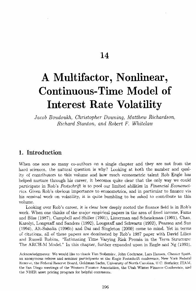
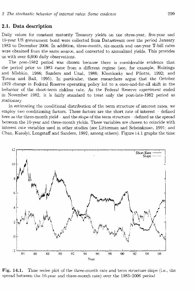
In estimating the conditional distribution of the term structure of interest rates, we employ two conditioning factors. These factors are the short rate of interest - defined here as the three-month yield - and the slope of the term structure - defined as the spread between the 10-year and three-month yields. These variables are chosen to coincide with interest rate variables used in other studies (see Litterman and Scheinkman, 1991; and Chan, Karolyi, Longstaff and Sanders, 1992, among others). Figure 14.1 graphs the time

Short Rate --Slope ....... .

84 86 88 90 92 94 96 98 00 02 04 06

Year

Fig. 14.1. Time series plot of the three-month rate and term structure slope (i.e., the spread between the 10-year and three-month rate) over the 1983-2006 period

300 A multifactor, nonlinear, continuous-time model of interest rate volatility

4r---------.----------.----------.-------~._~~----_.----,

3

2

o

+ + +

'*'

+ +

+-l"i- ++tit-.t + r'" + +

+ +-Pt-+* ++ +

+

+ + + t\ +

T + +

+f _1~ ________ ~ ________ ~ __________ L_ ______ ~~~~----~L---~

o 2 4 6

Short Rate

8 10

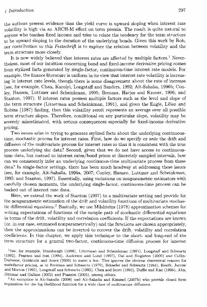
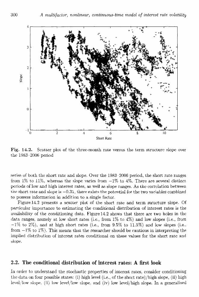
Fig. 14.2. Scatter plot of the three-month rate versus the term structure slope over the 1983-2006 period

series of both the short rate and slope. Over the 1983-2006 period, the short rate ranges from 1% to 11%, whereas the slope varies from -1% to 4%. There are several distinct periods of low and high interest rates, as well as slope ranges. As the correlation between the short rate and slope is -0.31, there exists the potential for the two variables combined to possess information in addition to a single factor.

Figure 14.2 presents a scatter plot of the short rate and term structure slope. Of particular importance to estimating the conditional distribution of interest rates is the availability of the conditioning data. Figure 14.2 shows that there are two holes in the data ranges, namely at low short rates (Le., from 1% to 4%) and low slopes (Le., from -1% to 2%), and at high short rates (Le., from 9.5% to 11.5%) and low slopes (Le., from -1 % to 1%). This means that the researcher should be cautious in interpreting the implied distribution of interest rates conditional on these values for the short rate and slope.

2.2. The conditional distribution of interest rates: A first look

In order to understand the stochastic properties of interest rates, consider conditioning the data on four possible states: (i) high level (Le., of the short rate)/high slope, (ii) high level/low slope, (ii) low level/low slope, and (iv) low level/high slope. In a generalized

'Jlatility

,t +

+ it-+

1-r+ r

*

+

+

Je over

ranges iistinct etween nbined

'pe. Of ; is the in the

" from ~s (i.e., ing the ~te and

tioning i) high ralized

2 The stochastic behavior of interest rates: Some evidence 301

method of moments framework, the moment conditions are:3

(.6.iT,t+ 1 - Jihr:hJ x It,hr:hs

(.6.iT,t+l-P:hr:ls) x It,hr:ls

(.6.iT,t+ 1 - J-llr:ls) x It,lr:ls

(.6.iT,t+l - J-llr:hs) X It,lr:hs

E [ (.6. 'T T) 2 T 2 X It,hr:hs = 0, (1)

'tt,t+l - J-lhr:hs - O"hr:hs

[ ( .6. 'T T) 2 T 2 X It,hr:ls 'tt,t+l - J-lhr:ls - (J" hr:ls

[(.6.'T T)2 T 2 X It,lr:ls 1,t,t+l - J-llr:l s - O"lr:ls

[ ( .6. 'T T) 2 T 2 X It,lr:hs 'tt,t+l - J-llr:hs - O"lr:hs

where .6.iT,t+l is the change in the T-period interest rate from t to t + 1, J-l~, is the mean change in rates conditional on one of the four states occurring, (J"~, is the volatility of the change in rates conditional on these states, and I t ,\, = 1 if [,1,] occurs, zero otherwise. These moments, J-lT and (J"T, thus represent coarse estimates of the underlying conditional moments of the distribution of interest rates.

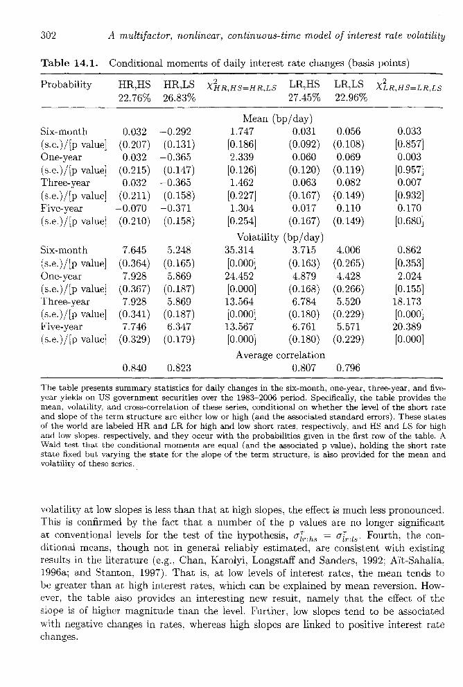
These moment conditions allow us to test a variety of restrictions. First, are (J"hr:hs = O"hr:ls and O"lr:hs = (J"lr:ls? That is, does the slope of the term structure help explain volatility at various interest rate levels? Second, similarly, with respect to the mean, are J-lhr:hs = J-lhr:ls and J-llr:hs = J-llr:ls? Table 14.1 provides estimates of J-l~, and (J"~" and the corresponding test statistics. Note that the framework allows for autocorrelation and heteroskedasticity in the underlying squared interest rate series when calculating the variance-covariance matrix of the estimates. Further, the cross­correlation between the volatility estimates is taken into account in deriving the test statistics.

Several facts emerge from Table 14.1. First, as documented by others (e.g., Chan, Karolyi, Longstaff and Sanders, 1992; and A'it-Sahalia, 1996a), interest rate volatility is increasing in the short rate of interest. Of some interest here, this result holds across the yield curve. That is, conditional on either a low or high slope, volatility is higher for the six-month, one-year, three-year and five-year rates at higher levels of the short rate. Second, the slope also plays an important role in determining interest rate volatil­ity. In particular, at high levels of interest rates, the volatility of interest rates across maturities is much higher at steeper slopes. For example, the six-month and five-year volatilities rise from 5.25 and 6.35 to 7.65 and 7.75 basis points, respectively. Formal tests of the hypothesis O"hr:hs = (J"hr:ls provide 1% level rejections at each of the maturi­ties. There is some evidence in the literature that expected returns on bonds are higher for steeper term structures (see, for example, Fama, 1986, and Boudoukh, Richardson, Smith and Whitelaw, 1999a, 1999b); these papers and the finding of Engle, Lilien and Robins (1987) may provide a link to the volatility result here. Third, the effect of the slope is most important at high interest rate levels. At low short rate levels, though the

3We define a low (high) level or slope as one that lies below (above) its unconditional mean, Here, this mean is being treated as a known constant, though, of course, it is estimated via the data,

302 A multifactor, nonlinear, continuous-time model of interest rate volatility

Table 14.1. Conditional moments of daily interest rate changes (basis points)

Probability HR,HS HR,LS 2 XHR,HS=HR,LS LR,HS LR,LS 2

XLR,H S=LR,LS

22.76% 26.83% 27.45% 22.96%

Mean (bpjday) Six-month 0.032 -0.292 1.747 0.031 0.056 0.033 (s.e.)j[p value] (0.207) (0.131) [0.186] (0.092) (0.108) [0.857] One-year 0.032 -0.365 2.339 0.060 0.069 0.003 (s.e.)j[p value] (0.215) (0.147) [0.126] (0.120) (0.119) [0.957] Three-year 0.032 -0.365 1.462 0.063 0.082 0.007 (s.e.)j[p value] (0.211) (0.158) [0.227] (0.167) (0.149) [0.932] Five-year -0.070 -0.371 1.304 0.017 0.110 0.170 (s.e.)j[p value] (0.210) (0.158) [0.254] (0.167) (0.149) [0.680]

Volatility (bpjday) Six-month 7.645 5.248 35.314 3.715 4.006 0.862 (s.e.)j[p value] (0.364) (0.165) [0.000] (0.163) (0.265) [0.353] One-year 7.928 5.869 24.452 4.879 4.428 2.024 (s.e.)j[p value] (0.367) (0.187) [0.000] (0.168) (0.266) [0.155] Three-year 7.928 5.869 13.564 6.784 5.520 18.173 (s.e.)j[p value] (0.341) (0.187) [0.000] (0.180) (0.229) [0.000] Five-year 7.746 6.347 13.567 6.761 5.571 20.389 (s.e.)j[p value] (0.329) (0.179) [0.000] (0.180) (0.229) [0.000]

Average correlation 0.840 0.823 0.807 0.796

The table presents summary statistics for daily changes in the six-month, one-year, three-year, and five­year yields on US government securities over the 1983-2006 period. Specifically, the table provides the mean, volatility, and cross-correlation of these series, conditional on whether the level of the short rate and slope of the term structure are either low or high (and the associated standard errors). These states of the world are labeled HR and LR for high and low short rates, respectively, and HS and LS for high and low slopes, respectively, and they occur with the probabilities given in the first row of the table. A Wald test that the conditional moments are equal (and the associated p value), holding the short rate state fixed but varying the state for the slope of the term structure, is also provided for the mean and volatility of these series.

volatility at low slopes is less than that at high slopes, the effect is much less pronounced. This is confirmed by the fact that a number of the p values are no longer significant at conventional levels for the test of the hypothesis, CJlr:hs = CJ1r:ls ' Fourth, the con­ditional means, though not in general reliably estimated, are consistent with existing results in the literature (e.g., Chan, Karolyi, Longstaff and Sanders, 1992; Ait-Sahalia, 1996a; and Stanton, 1997). That is, at low levels of interest rates, the mean tends to be greater than at high interest rates, which can be explained by mean reversion. How­ever, the table also provides an interesting new result, namely that the effect of the slope is of higher magnitude than the level. Further, low slopes tend to be associated with negative changes in rates, whereas high slopes are linked to positive interest rate changes.

volatility

s)

rS=LR,LS

.033

.857]

.003

.957]

.007

.932]

.170

.680]

. 862

.353]

. 024

.155]

.173

.000]

.389

.000]

r, and five­rovides the ~ short rate 'hese states lS for high he table. A , short rate , mean and

nounced. 19nificant the con-existing

-Sahalia, tends to

::m. How­ct of the 3sociated :rest rate

2 The stochastic behavior of interest rates: Some evidence 303

2.3. The conditional distribution of interest rates: A closer look

In order to generalize the results of Section 2.2, we employ a kernel estimation pro­cedure for estimating the relation between interest rate changes and components of the term-structure of interest rates. Kernel estimation is a nonparametric method for estimating the joint density of a set of random variables. Specifically, given a time series Lli[,t+l' ir and i~ (where i r is the level of interest rates, and is is the slope), generated from an unknown density f(Lli 7

, ir , is), then a kernel estimator of this density is

(2)

where K ( .) is a suitable kernel function and h is the window width or smoothing parameter .

We employ the commonly used independent multivariate normal kernel for K(-). The other parameter, the window width, is chosen based on the dispersion of the observations . For the independent multivariate normal kernel, Scott (1992) suggests the window width,

where (;-i is the standard deviation estimate of each variable Zi, T is the number of observations, m is the dimension of the variables, and k is a scaling constant often chosen via cross-validation. Here, we employ a cross-validation procedure to find the k that provides the right trade-off between the bias and variance of the errors. Across all the data points, we find the ks that minimize the mean-squared error between the observed data and the estimated conditional data. This mean-squared error minimization is implemented using a Jackknife-based procedure. In particular, the various implied conditional moments at each data point are estimated using the entire sample, except for the actual data point and its nearest neighbors.4 Once the k is chosen, the actual estimation of the conditional distribution of interest rates involves the entire sample, albeit using window widths chosen from partial samples. To coincide with Section 2.2., we focus on the first two conditional moments of the distribution, and it is possible to show that

T

A (.r 'S) '" ('r 'S);\'7 l-".6.i T 2 ,2 = ~ Wt 2 ,2 Ll'/,t (3) t=l

(4)

-lDue to the serial dependence of the data, we performed the cross-validation omitting 100 observations, i.e., four months in either direction of the particular data point in question. Depending on the moments in question, the optimal ks range from roughly 1.7 to 27.6, which implies approximately twice to 28 times the smoothing parameter of Scott's asymptotically optimal implied value.

304

9

8.5

8

7.5

7

6.5

6

5.5

5

4.5

A multifactor, nonlinear, continuous-time model of interest rate volatility

Volatility (bp/day) (One year)

0.01 0.005

0.02

0.035 0.03

0.025

0.015 Slope

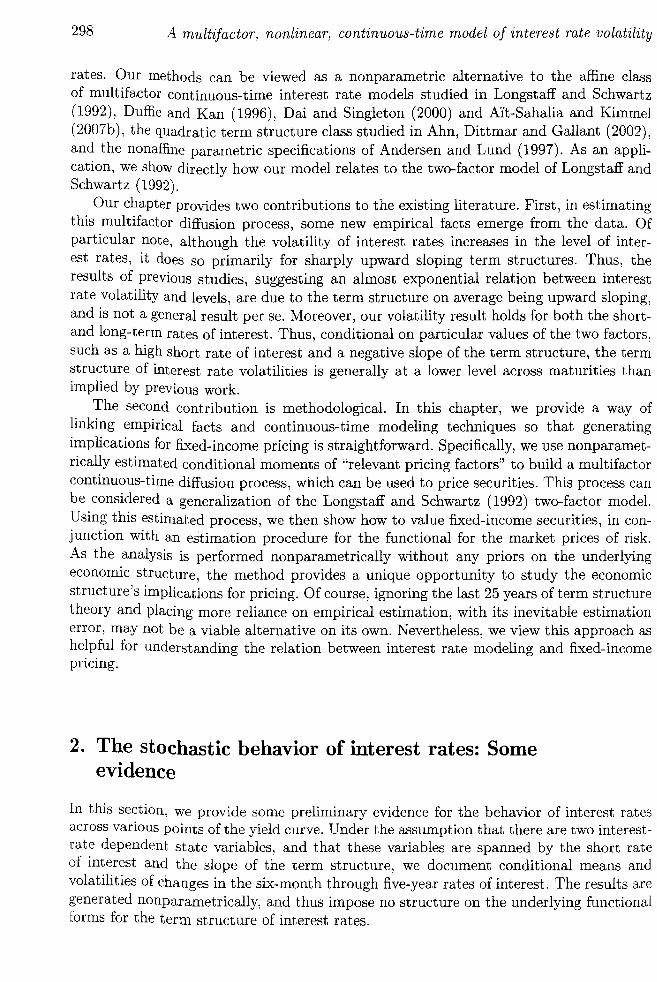
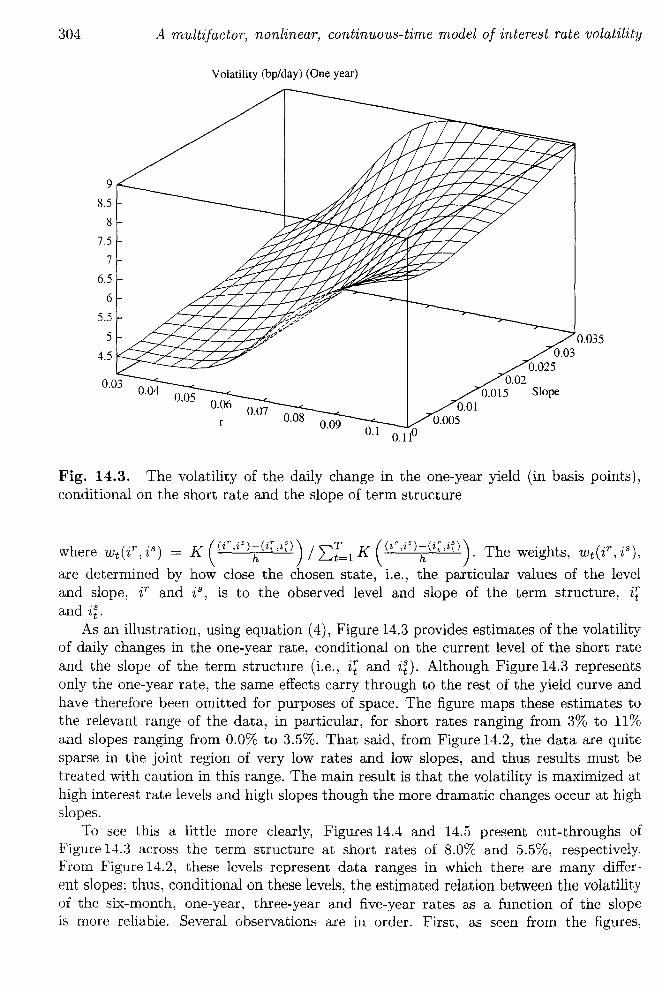
Fig. 14.3. The volatility of the daily change in the one-year yield (in basis points), conditional on the short rate and the slope of term structure

where WtW', is) = K (W,iS)~(i; ,it)) / 'L'[=1 K «ir'iS)~(i~'it)). The weights, Wt(iT, is),

are determined by how close the chosen state, i.e., the particular values of the level and slope, iT and is, is to the observed level and slope of the term structure, ir and i:.

As an illustration, using equation (4), Figure 14.3 provides estimates of the volatility of daily changes in the one-year rate, conditional on the current level of the short rate and the slope of the term structure (Le., ir and in. Although Figure 14.3 represents only the one-year rate, the same effects carry through to the rest of the yield curve and have therefore been omitted for purposes of space. The figure maps these estimates to the relevant range of the data, in particular, for short rates ranging from 3% to 11% and slopes ranging from 0.0% to 3.5%. That said, from Figure 14.2, the data are quite sparse in the joint region of very low rates and low slopes, and thus results must be treated with caution in this range. The main result is that the volatility is maximized at high interest rate levels and high slopes though the more dramatic changes occur at high slopes.

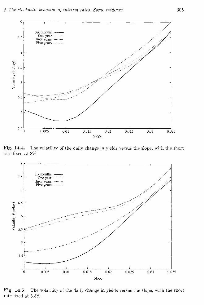
To see this a little more clearly, Figures 14.4 and 14.5 present cut-throughs of Figure 14.3 across the term structure at short rates of 8.0% and 5.5%, respectively. From Figure 14.2, these levels represent data ranges in which there are many differ­ent slopes; thus, conditional on these levels, the estimated relation between the volatility of the six-month, one-year, three-year and five-year rates as a function of the slope is more reliable. Several observations are in order. First, as seen from the figures,

-

atility

lints),

r ·s) ,2 ,

level

ltility t rate ;sents e and ~es to ,11% quite st be :ed at

high

hs of ively. iiffer­ttility slope sures,

2 The stochastic behavior oj interest rates: Some evidence

~ «I

9r-------.--------.------~--------r_------,_------_r------~

g.5 Six months -­

One year ------­Three years

Five years

,/ ,/

;""",

/ ,/

",,;"';/

,,"//

".-,,/ ."

=a 7.5 """" ,," ." e "' .. ,:.:.(:.::.:.: ....... .

:)');// .. - .. /

,,'

" ..................... --:.-.-=...., .. -..... . ..:.:.: ............ -_ •.•.

6.5

6

5.5k-------L-----~L-____ ~ ______ ~ ______ ~ ______ ~ ______ ~ o 0.005 0.01 0.Dl5 0.02 0.025 0.03 0.035

Slope

305

Fig. 14.4. The volatility of the daily change in yields versus the slope, with the short rate fixed at 8%

g,-------,-------_r-------,--------,-------,--------,-------,

Six months --7.5 One year -------

Three years Five years ............... .

7

~ 6.5 «I

:s:: c..

~ 6 ........................................... .

.............. -; " .......... . ~ 5.5 .~.~ .. :~.~.~ .. :~~~ .. .

5

4.5

4k-------~----__ -L ______ ~ ________ ~ ______ ~ ______ ~ ______ ~

o 0.005 0.01 0.Dl5 0.02 0.025 0.03 0.035

Slope

Fig. 14.5. The volatility of the daily change in yields versus the slope, with the short rate fixed at 5.5%

306 A multifactor, nonlinear, continuous-time model of interest rate volatility

9

8.5 Six months --

8 Th

One year ------- .--___ ' ree years ........ /"

Five years ................ /

7.5

~ ;>. 7 <':l :a 6

~ 6.5

.~ " ... ;,,,//

C 6 ;>

... ;,,;

,,' ".-,,///

5.5 " ... ",----" ...... --

................

--5

4.5

4L-____ ~ ______ -L ______ ~ ____ ~~ ____ _4 ______ ~ ______ L_ ____ ~

0.03 0.04 0.05 0.06 0.07 0.08 0.09 0.1 0.11 r

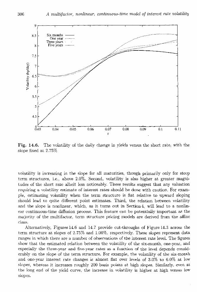
Fig. 14.6. The volatility of the daily change in yields versus the short rate, with the slope fixed at 2.75%

volatility is increasing in the slope for all maturities, though primarily only for steep term structures, i.e., above 2.0%. Second, volatility is also higher at greater magni­tudes of the short rate albeit less noticeably. These results suggest that any valuation requiring a volatility estimate of interest rates should be done with caution. For exam­ple, estimating volatility when the term structure is flat relative to upward sloping should lead to quite different point estimates. Third, the relation between volatility and the slope is nonlinear, which, as it turns out in Section 4, will lead to a nonlin­ear continuous-time diffusion process. This feature can be potentially important as the majority of the multifactor, term structure pricing models are derived from the affine class.

Alternatively, Figures 14.6 and 14.7 provide cut-throughs of Figure 14.3 across the term structure at slopes of 2.75% and 1.00%, respectively. These slopes represent data ranges in which there are a number of observations of the interest rate level. The figures show that the estimated relation between the volatility of the six-month, one-year, and especially the three-year and five-year rates as a function of the level depends consid­erably on the slope of the term structure. For example, the volatility of the six-month and one-year interest rate changes is almost fiat over levels of 3.0% to 6.0% at low slopes, whereas it increases roughly 200 basis points at high slopes. Similarly, even at the long end of the yield curve, the increase in volatility is higher at high versus low slopes.

e volatility

0.11

, with the

for steep ~r magni­valuation "or exam­d sloping volatility a nonlin­,nt as the the affine

.cross the sent data he figures year, and ls consid­ix-month 70 at low ~ even at ::fSUS low

3 Estimation of a continuous-time multifactor diffusion process

§ 3

8r------.------.-----~------._----_,r_----_r------r_----_,

7.5

7

Six months -­One year -------

Three years ....... . Five years ............... .

/

/"" ......... ",,,,/"

.///// ............... .

/.< ................................................... .

/::""",,,--,::>,;;/>_ ___--1

6 ....................... . .. . ................................................................

>0 - 5 ).

.................. -'"""",,"//

/,/,//

-' -,' ,-' 5

4.5

4~-----L------~----~------~----~~-----L------~----~ 0.03 0.04 0.05 0.06 0.07 0.08 0.09 0.1 0.11

r

307

Fig. 14.7. The volatility of the daily change in yields versus the short rate, with the slope fixed at 1%

3. Estimation of a continuous-time multifactor diffusion process

The results of Section 2 suggest that the volatility of changes in the term structure of interest rates depends on at least two factors. Given the importance of continuous-time mathematics in the fixed income area, the question arises as to how these results can be interpreted in a continuous-time setting. Using data on bond prices, and explicit theo­retical pricing models (e.g., Cox, Ingersoll and Ross, 1985), Brown and Dybvig (1986), Pearson and Sun (1994), Gibbons and Ramaswamy (1993) and Dai and Singleton (2000) all estimate parameters of the underlying interest rate process in a fashion consistent with the underlying continuous-time model. These procedures limit themselves, however, to fairly simple specifications.

As a result, a literature emerged which allows estimation and inference of fairly general continuous-time diffusion processes using discretely sampled data. Ait-Sahalia (2007) provides a survey of this literature and we provide a quick review here. First, at a parametric level, there has been considerable effort in the finance literature at working through maximum likelihood applications of continuous-time processes with discretely sampled data, starting with Lo (1988) and continuing more recently with Ait-Sahalia (2002) and Ait-Sahalia and Kimmel (2007a, 2007b). Second, by employ­ing the infinitesimal generators of the underlying continuous-time diffusion processes, Hansen and Scheinkman (1995) and Conley, Hansen, Luttmer and Scheinkman (1995)

-_ .... 308 A multifactor, nonlinear, continuous-time model of interest rate volatility

construct moment conditions that also make the investigation of continuous-time mod­els possible with discrete time data. Third, in a nonparametric framework, Ait-Sahalia (1996a, 1996b) develops a procedure for estimating the underlying process for interest rates using discrete data by choosing a model for the drift of interest rates and then non parametrically estimating its diffusion function. Finally, as an alternative method, Stanton (1997) employs approximations to the true drift and diffusion of the underly­ing process, and then nonparametrically estimates these approximation terms to back out the continuous-time process (see also Bandi, 2002; Chapman and Pearson, 2000; and Pritsker, 1998). The advantage of this approach is twofold: (i) similar to the other procedures, the data need only be observed at discrete time intervals, and (ii) the drift and diffusion are unspecified, and thus may be highly nonlinear in the state variable.

In this section, we extend the work of Stanton (1997) to a multivariate setting and provide for the nonparametric estimation of the drift and volatility functions of multi­variate stochastic differential equations. Similar to Stanton (1997), we use Milshtein's (1978) approximation schemes for writing expectations of functions of the sample path of stochastic differential equations in terms of the drift and volatility coefficients. If the expectations are known (albeit estimated nonparametrically in this paper) and the functions are chosen appropriately, then the approximations can be inverted to recover the drift and volatility coefficients. We have performed an extensive simulation analysis (not shown here) to better understand the properties of the estimators. Not surprisingly, the standard errors around the estimators, as well as the properties of the goodness of fit, deteriorate as the data becomes more sparse. Given the aforementioned literature that looks at univariate properties of interest rates, it is important to point out that these properties suffer more in the multivariate setting as we introduce more "Star trek" regions of the data with the increasing dimensionality of the system. Nevertheless, this point aside, the approximation results here for the continuous-time process carry through to those presented in Stanton (1997), in particular, the first order approximation works well at daily to weekly horizons, while higher order approximations are required for less frequent sampling.

3.1. Drift, diffusion and correlation approximations

Assume that no arbitrage opportunities exist, and that bond prices are functions of two state variables, the values of which can always be inverted from the current level, Rt ,

and a second state variable, St. Assume that these variables follow the (jointly) Markov diffusion process

dRt = f.1R(Rt , St) dt + CYR(Rt , St) dzf

dSt = f.1s(Rt , St) dt + cys(Rt, St) dzf,

(5)

(6)

where the drift, volatility and correlation coefficients (i.e., the correlation between ZR and ZS) all depend on Rt and St. Define the vector X t = (Rt, St).

Q

volatility

ne mod­-Sahalia interest

.nd then method, underly­to back

[1, 2000; . to the and (ii) he state

.ing and ,f multi­lshtein's )le path .ents. If and the recover

analysis risingly, iness of ;erature ,ut that 1r trek" ~ss, this ;hrough .1 works for less

; of two /el, Rt ,

vlarkov

(5)

(6)

~en ZR

3 Estimation of a continuous-time multifactor diffusion process 309

Under suitable restrictions on M, (J, and a function f, we can write the conditional expectation E t [J(Xt+.d)] in the form of a Taylor series expansion,5

1 2 2 E t [J(Xt+.d)] = f(Xt ) + £f(Xt) 6. + 2£ f(Xt)6. + ...

+ ~£n f(Xd6.n + O(6.n+1), n.

(7)

where £ is the infinitesimal generator of the multivariate process {Xd (see 0ksendal, 1985; and Hansen and Scheinkman, 1995), defined by

where

Equation (7) can be used to construct numerical approximations to Etlf(Xt+.d)] in the form of a Taylor series expansion, given known functions MR, Ms, p, (JR and (JS (see, for example, Milshtein, 1978). Alternatively, given an appropriately chosen set of functions f(·) and nonparametric estimates of Edf(Xt+.d)], we can use equation (7) to construct approximations to the drift, volatility and correlation coefficients (i.e., M R, M s, p, (J Rand (J s) of the underlying multifactor, continuous-time diffusion pro­cess. The nice feature of this method is that the functional forms for MR, Ms, p, (JR and (J S are quite general, and can be estimated nonparametrically from the underlying data. Rearranging equation (7), and using a time step of length i6.( i = 1,2, ... ), we obtain

~. 1 E~(Xt) == i6. Et [J(Xt+i.d) - f(Xt}] ,

= £f(Xt) + ~£2 f(Xt)(i6.) + ... + ~£n f(Xt)(i6.t-1 + O(6.n). (8)

2 n.

From equation (8), each of the Ei is a first order approximation to £f,

5For a discussion see, for example, Hille and Phillips (1957), Chapter 1l. Milshtein (1974, 1978) gives examples of conditions under which this expansion is valid, involving bounded ness of the functions /1, 17,

f and their derivatives. There are some stationary processes for which this expansion does not hold for the functions f that we shall be considering, including processes such as

dx = /1dt + x 3 dZ,

which exhibit "volatility induced stationary" (see Conley, Hansen, Luttmer and Scheinkman, 1995). However, any process for which the first order Taylor series expansion fails to hold (for linear f) will also fail if we try to use the usual numerical simulation methods (e.g. Euler discretization). This severely limits their usefulness in practice.

310 A multifactor, nonlinear, continuous-time model of interest rate volatility

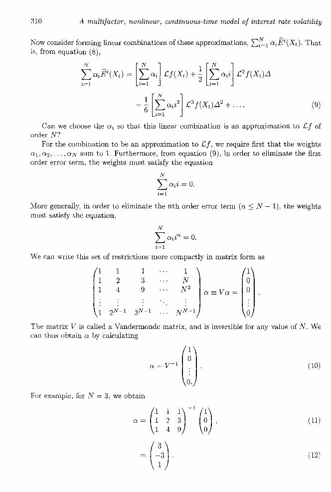
N ow consider forming linear combinations of these approximations, "L:[: 1 aJEi (Xt ). That is, from equation (8),

(9)

Can we choose the ai so that this linear combination is an approximation to £ j of order N?

For the combination to be an approximation to £j, we require first that the weights aI, a2,"" aN sum to 1. Furthermore, from equation (9), in order to eliminate the first order error term, the weights must satisfy the equation

N

L aii = O. i=l

More generally, in order to eliminate the nth order error term (n ~ N - 1), the weights must satisfy the equation,

N

L aiin = O. i=l

We can write this set of restrictions more compactly in matrix form as

1 1 1 1 1 1 2 3 N 0 1 4 9 N 2

a=Va= 0

1 2N - l 3N - l NN-l 0

The matrix V is called a Vandermonde matrix, and is invertible for any value of N. We can thus obtain a by calculating

(10)

For example, for N = 3, we obtain

(11)

(12)

JQlatility

t). That

(9)

J £f of

weights the first

weights

f N. VVe

(10)

(ll)

(12)

-! I

3 Estimation of a continuous-time multifactor diffusion process 311

Substituting 0: into equation (9), and using equation (8), we get the following third order approximation of the infinitesimal generator of the process {Xd:

1 £f(Xt) = 6.1 [18Et (f(Xt+L1 ) - f(Xt)) - 9Et (f(Xt+2L1 ) - f(Xd)

+ 2Et (f(Xt+3L1 ) - f(Xt ))] + 0(.13).

To approximate a particular function g( x), we now need merely to find a specific function f satisfying

£f(x) = g(x).

For our purposes, consider the functions

f(1) (R) == R - Rt ,

f(2)(S) == S - St,

f(3)(R) == (R - Rt )2 ,

2 f(4) (S) == (S - St) ,

f(5) (R, S) == (R - Rt) (S - St) .

From the definition of £, we have

£f(1) (R) = /-LR(R, S),

£f(2) (S) = /-Ls(R, S),

£f(3)(R) = 2(R - Rt)/-LR(R, S) + O"~(R, S),

£f(4) (S) = 2(S - St)/-Ls(R, S) + (J~(R, S),

£f(5)(R, S) = (S - St)/-LR(R, S) + (R - Rt)/-Ls(R, S) + p(R, S)O"R(R, S)O"s(R, S).

Evaluating these at R = Rt , S = St, we obtain

£f(1) (Rt) = /-LR (Rt, St),

£f(2) (St) = /-Ls(Rt, St),

£f(3)(Rt) = O"~(Rt, St),

£f(4) (St) = (J~(Rt, St),

£f(5) (Rt, St) = p(Rt, SdO"R(Rt , St)O"s(Rt, St).

Using each of these functions in turn as the function f above, we can generate approxima­tions to /-LR, /-Ls, (JR, O"s and p respectively. For example, the third order approximations

312 A multifactor, nonlinear, continuous-time model of interest rate volatility

(taking square roots for CT Rand CT S) are

1 IlR(Rt , St) = 6,1 [18Et (Rt+L1 - Rt) - gEt (Rt+2L1 - Rt ) + 2Et (RH3 L1 - Rt )]

+ 0(,13),

1 Ils(Rt , St) = 6,1 [18Et (SHL1 - St) - gEt (SH2L1 - Sd + 2Et (SH3L1 - St)]

+ 0(,13),

1 6,1 (

18Et [(Rt+L1 - Rt )2] - gEt [(Rt+2L1 - Rt)2]

+2Et [(Rt+3 L1 - Rt)2]

~ ( 18Et [CSHL1 - St)2] - gEt [CSH2L1 - St)2]

6,1 +2Et [CSH3L1 - St)2]

1 CTRS(Rt , St) = 6,1 (18Et [(RHL1 - Rt ) (SHL1 - St)]

- gEt [(RH2L1 - Rt ) (SH2L1 - St)]

+2Et [(RH3L1 - Rt ) (SH3L1 - St)]) .

) )

(13)

The approximations of the drift, volatility and correlation coefficients are written in terms of the true first, second and cross moments of multiperiod changes in the two state variables. If the two-factor assumption is appropriate, and a large stationary time series is available, then these conditional moments can be estimated using appropriate nonparametric methods. In this chapter, we estimate the moments using multivariate density estimation, with appropriately chosen factors as the conditioning variables. All that is required is that these factors span the same space as the true state variables.6 The results for daily changes were provided in Section 2. Equation (13) shows that these esti­mates are an important part of the approximations to the underlying continuous-time dynamics. By adding multiperiod extensions of these nonparametric estimated condi­tional moments, we can estimate the drift, volatility and correlation coefficients of the multifactor process described by equations (5) and (6).

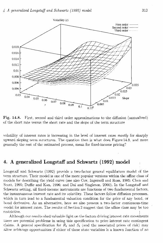
Figure 14.8 provides the first, second and third order approximations to the diffusion of the short rate against the short rate level and the slope of the term structure. 7 The most notable result is that a first order approximation works well; thus, one can consider the theoretical results of this section as a justification for discretization methods cur­rently used in the literature. The description of interest rate behavior given in Section 2, therefore, carries through to the continuous-time setting. Our major finding is that the

6See Duffie and Kan (1996) for a discussion of the conditions under which this is possible (in a linear setting).

7Figures showing the various approximations to the drift of the short rate, the drift and diffusion of the slope, and the correlation between the short rate and the slope are available upon request.

.....,.. I

ity ! 4 A generalized Longstaff and Schwartz {1992} model 313

~n in two

time Iriate ~riate

;. All i The ~ esti­-time :ondi­)f the

~usion

7 The Qsider s cur­tion 2. at the

1 linear

lsion of

0.018

0.016

0.014

0.012

0.01

0.008 ..,..-~./----

0.006

0.004

Volatility (r)

First order -­Second order ------­

Third order .-------

0.02 0.015

0.01 0.005

0.Q35 0.03

0.025

Slope

Fig. 14.8. First, second and third order approximations to the diffusion (annualized) of the short rate versus the short rate and the slope of the term structure

volatility of interest rates is increasing in the level of interest rates mostly for sharply upward sloping term structures. The question then is what does Figure 14.8, and more generally the rest of the estimated process, mean for fixed-income pricing?

4. A generalized Longstaff and Schwartz {1992} model

Longstaff and Schwartz (1992) provide a two-factor general equilibrium model df the term structure. Their model is one of the more popular versions within the affine class of models for describing the yield curve (see also Cox, Ingersoll and Ross, 1985; Chen and Scott, 1995; Duffie and Kan, 1996; and Dai and Singleton, 2000). In the Longstaff and Schwartz setting, all fixed-income instruments are functions of two fundamental factors, the instantaneous interest rate and its volatility. These factors follow diffusion processes, which in turn lead to a fundamental valuation condition for the price of any bond, or bond derivative. As an alternative, here we also present a two-factor continuous-time model for interest rates. The results of Section 2 suggest that the affine class may qe too restrictive. I

Although our results shed valuable light on the factors driving interest rate movements there are potential problems in using this specification to price interest rate contingent claims. A general specification for R t and St (and the associated prices of risk) may allow arbitrage opportunities if either of these state variables is a known function of an

314 A multifactor, nonlinear, continuous-time model of interest rate volatility

asset price.8 Of course, this point is true of all previous estimations of continuous-time processes to the extent that they use a priced proxy as the instantaneous rate. If we are willing to assume that we have the right factors, however, then there is no problem in an asymptotic sense. That is, as we are estimating these processes nonparametrically, as the sample size gets larger, our estimates will converge to the true functions, which are automatically arbitrage-free (if the economy is). Nevertheless, this is of little consolation if we are trying to use the estimated functions to price assets.

To get around this problem, we need to write the model in a form in which neither state variable is an asset price or a function of asset prices. In this chapter, we follow convention by using the observable three-month yield as a proxy for the instantaneous rate, Rt . Furthermore, suppose that the mapping from (R, S) to (R,O"R) is invertible,9 so we can write asset prices as a function of Rand 0" R, instead of Rand S. 10 As 0" R is not an asset price, using this variable avoids the inconsistency problem.

Specifically, suppose that the true model governing interest rate movements is a generalization of the two-factor Longstaff and Schwartz (1992) model,

dRt = J-LR(R, 0") dt + 0" dZ1 ,

dO"t = J-La(R, O")dt + p(R, O")s(R, 0") dZ1 + v'l- p2 8 dZ2 ,

where dZ1 dZ2 = O.ll In vector terms,

d(Rt,O"t) = !vI dt + e dZ,

where

!vI == (~:) ,

e == (;8 J 1 ~ p2 8) .

(14)

(15)

Asset prices, and hence the slope of the term structure, can be written as some function of the short rate and instantaneous short rate volatility, S(R, 0").

From equations (14) and (15), how do we estimate the underlying processes for R and 0" given the estimation results of Section 3? Although the short rate volatility, 0", is not directly observable, it is possible to estimate this process. Specifically, using Ito's

8See , for example, Duffie, Ma and Yong (1995). The problem is that, given such a model, we can price any bond, and are thus able to calculate what the state variable "ought" to be. Without imposing any restrictions on the assumed dynamics for R t and St, there is no guarantee that we will get back to

the same value of the state variable that we started with. 9That is, for a given value of Rt, the volatility, JR, is monotonic in the slope, S. This is the case in

most existing multifactor interest rate models, including, for example all affine models, such as Longstaff and Schwartz (1992).

loThis follows by writing

V(R, S) = V(R, S(R, JR)) == U(R, JR)'

11 This specification is the most convenient to deal with, as we now have orthogonal noise terms. The correlation between the diffusion terms is p, and the overall variance of J is 8 2 dt.

)latility

ls-time we are

)lem in ally, as ich are olation

neither follow

aneous rtible.9

s UR is

ts is a

(14)

(15 )

mction

; for R y, U. IS

g Ito's

we can nposing back to

. case in ongstaff

ns. The

4 A generalized Longstaff and Schwartz {1992} model

Lemma, together with estimates for I1R, uR, I1s, uS and p, it is possible to write

dut = uRdRt + usdSt + ~ [uRRu2 (Rt , St) + ussu~(Rt, St)

+2uRsu(Rt , St)us(Rt , St)p(Rt, St)] dt.

315

Given this equation, and the assumption that the function S(R, u) is invertible, the dynamics of Ut can be written as a function of the current level of Rand u in a straightforward way.

This procedure requires estimation of a matrix of second derivatives. Although there are well-known problems in estimating higher order derivatives using kernel density estimation techniques, it is possible to link the results of Section 2 and 3 to this general­ized Longstaff and Schwartz (1992) model. In particular, using estimates of the second derivatives (not shown), several facts emerge. First, due to the small magnitudes of the estimated drifts of the state variables Rand S, the drift of u depends primarily on the second order terms. Consequently, the importance of the second factor (the slope) is determined by how much the sensitivity of short rate volatility to this factor changes relative to the changes in the sensitivity to the first factor (the level). The general pat­tern is that volatility increases at a slower rate for high levels and a faster rate for high slopes. Consequently, for high volatilities and levels, the drift of volatility is negative, generating mean reversion. The effect of the second factor, however, is to counter this phenomenon. Second, the diffusion of u is determined by the sensitivities of short rate volatility to the two factors and the magnitudes of the volatilities of the factors. Based on the estimates of the volatilities and derivatives, the slope has the dominant influ­ence on this effect. In particular, the volatility of u is high for upward sloping term structures, which also correspond to states with high short rate volatility. Moreover, sen­sitivity of this diffusion to the two factors is larger in the slope direction than in the level direction.

As an alternative to the above method, we can estimate an implied series for u by assuming that the function S(R, u) is invertible, i.e., that we can equivalently write the model in the form

dRt = I1R(Rt , St)dt + u(Rt, St)dZ;

dSt = I1s(Rt , St)dt + us(Rt , St)dZ~,

where Zi and Z2 may be correlated. To estimate the function u(R, S), we apply the methodology described in Section3.1 to the function i(3)(R, S) == (R - Rt)2. Apply­ing the estimated function to each observed (R, S) pair in turn yields a series for the volatility u, which we can then use in estimating the generalized Longstaff and Schwartz (1992) model given in equations (14) and (15).12 This procedure is in stark contrast to that of Longstaff and Schwartz (1992), and others, who approximate the dynamics of the volatility factor as a Generalized Autoregressive Conditional Heteroskedasticity (GARCH) process. The GARCH process is not strictly compatible with the underlying dynamics of their continuous-time model; here, the estimation is based on approximation

12 Although the use of an estimated series for (J rather than the true series may not be the most efficient approach, this procedure is consistent. That is, the problem will disappear as the sample size becomes large, and our pointwise estimates of (J converge to the true values.

316

0.015

0.014

0.013

0.012 (1j

E <:Jl

Ui 0.011

0.01

0.009

~~~-~~~---~----. ----~-

A multifactor, nonlinear, continuous-time model of interest rate volatility

0.04 0.05 0.06

+

0.07

Short rate

0.08 0.09 0.1 0.11

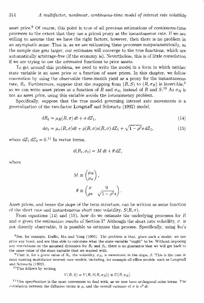
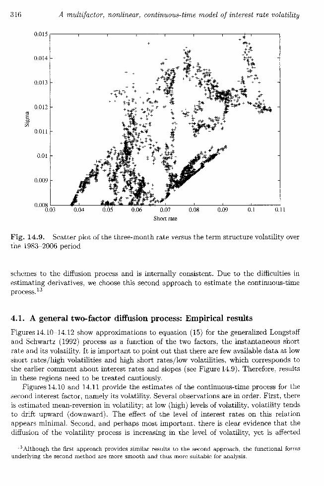
Fig. 14.9. Scatter plot of the three-month rate versus the term structure volatility over the 1983-2006 period

schemes to the diffusion process and is internally consistent. Due to the difficulties in estimating derivatives, we choose this second approach to estimate the continuous-time process. 13

4.1. A general two-factor diffusion process: Empirical results

Figures 14.10-14.12 show approximations to equation (15) for the generalized Longstaff and Schwartz (1992) process as a function of the two factors, the instantaneous short rate and its volatility. It is important to point out that there are few available data at low short rates/high volatilities and high short rates/low volatilities, which corresponds to the earlier comment about interest rates and slopes (see Figure 14.9). Therefore, results in these regions need to be treated cautiously.

Figures 14.10 and 14.11 provide the estimates of the continuous-time process for the second interest factor, namely its volatility. Several observations are in order. First, there is estimated mean-reversion in volatility; at low (high) levels of volatility, volatility tends to drift upward (downward). The effect of the level of interest rates on this relation appears minimal. Second, and perhaps most important, there is clear evidence that the diffusion of the volatility process is increasing in the level of volatility, yet is affected

13 Although the first approach provides similar results to the second approach, the functional forms underlying the second method are more smooth and thus more suitable for analysis.

'" I

volatility

(lll

ilityover

:ulties in ous-time

~ongstaff

lUS short ta at low ponds to 2. results

;s for the :st, there ity tends

relation that the affected

Jnal forms

4 A generalized Longstaff and Schwartz (1992) model

Drift (sigma)

o.ooo~ ~2:~~~~~~~~~~~~~~~~~~~~~::=;= -0.0001 ""'---...--

-0.0002 """, '" \ " " __ ' ___ " __ '_"-~~-~~~-:'-=--~~\~---:' -0.0003 " -::'::...--')...-~':....-,::~-:.::....-~:-- " --

-0.0004

-0.0005

-0.0006

-0.0007

-0.0008

-0.0009

0.015 0.014

0.013 0.012

0.011 0.01

0.009 Sigma 0.008

0.007 r 0.006 0.11 0.005

317

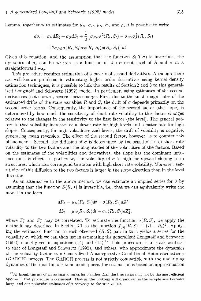
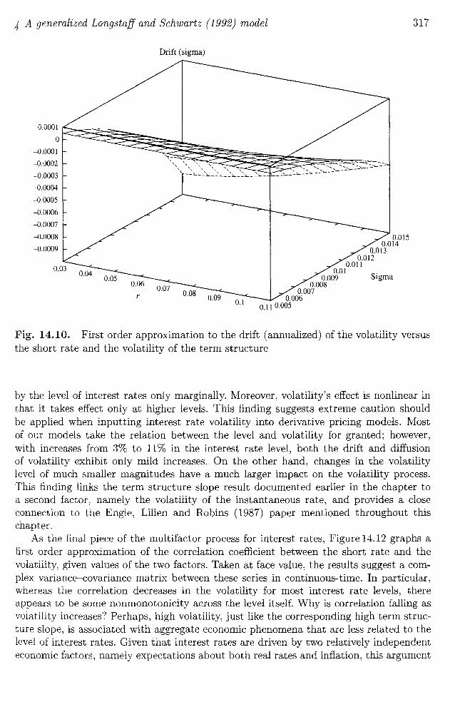
Fig. 14.10. First order approximation to the drift (annualized) of the volatility versus the short rate and the volatility of the term structure

by the level of interest rates only marginally. Moreover, volatility's effect is nonlinear in that it takes effect only at higher levels. This finding suggests extreme caution should be applied when inputting interest rate volatility into derivative pricing models. Most of our models take the relation between the level and volatility for granted; however, with increases from 3% to 11% in the interest rate level, both the drift and diffusion of volatility exhibit only mild increases. On the other hand, changes in the volatility level of much smaller magnitudes have a much larger impact on the volatility process. This finding links the term structure slope result documented earlier in the chapter to a second factor, namely the volatility of the instantaneous rate, and provides a close connection to the Engle, Lilien and Robins (1987) paper mentioned throughout this chapter.

As the final piece of the multifactor process for interest rates, Figure 14.12 graphs a first order approximation of the correlation coefficient between the short rate and the volatility, given values of the two factors. Taken at face value, the results suggest a com­plex variance-covariance matrix between these series in continuous-time. In particular, whereas the correlation decreases in the volatility for most interest rate levels, there appears to be some nonmonotonicity across the level itself. Why is correlation falling as volatility increases? Perhaps, high volatility, just like the corresponding high term struc­ture slope, is associated with aggregate economic phenomena that are less related to the level of interest rates. Given that interest rates are driven by two relatively independent economic factors, namely expectations about both real rates and inflation, this argument

318

0.009

0.008

0.007

0.006

0.005

O.OQ4

0.003

0.002

0.001

A multifactor, nonlinear, continuous-time model of interest rate volatility

Volatility (sigma)

o

0.015 0.014

O.Ol3 0.012

0.011 0.00~01 Sigma

0.008 0.007

r 0.09 0.006 0.11 0.005 0.1

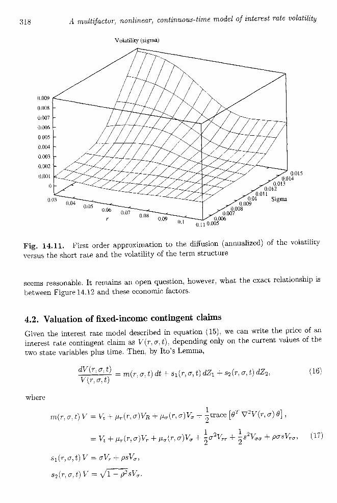
Fig. 14.11. First order approximation to the diffusion (annualized) of the volatility versus the short rate and the volatility of the term structure

seems reasonable. It remains an open question, however, what the exact relationship is between Figure 14.12 and these economic factors.

4.2. Valuation of fixed-income contingent claims Given the interest rate model described in equation (15), we can write the price of an interest rate contingent claim as V(r, cr, t), depending only on the current values of the two state variables plus time. Then, by Ito's Lemma,

dV(r,cr,t) ( )d () () V( )

= m r, cr, t t + S1 r, cr, t dZ1 + S2 r, cr, t dZ2, r, cr, t

(16)

where

1 m(r, cr, t) V = vt + J.Lr(r, cr)VR + J.La(r, cr)Va + 2"trace [aT \72V(r, cr) a] ,

r 1 2 1 2 = vt + J.Lr(r,cr)vr + J.La(r,cr)Va + 2"cr Vrr + 2"s Vaa + pcrsVra , (17)

S1 (r, cr, t) V = crVr + psVa,

s2(r, cr, t) V = }1 - p2sVa.

latility

5

ltility

hip is

of an )f the

(16)

(17)

4 A generalized Longstaff and Schwartz (1992) model

Correlation (r, sigma)

0.6

0.5

0.4

OJ

0.2

0.1

0

-0.1

r

0.015 0.014

0.013 0.012

0.011 0.01 Sigma

0.009 0.008

0.007 0.006

0.11 0.005

319

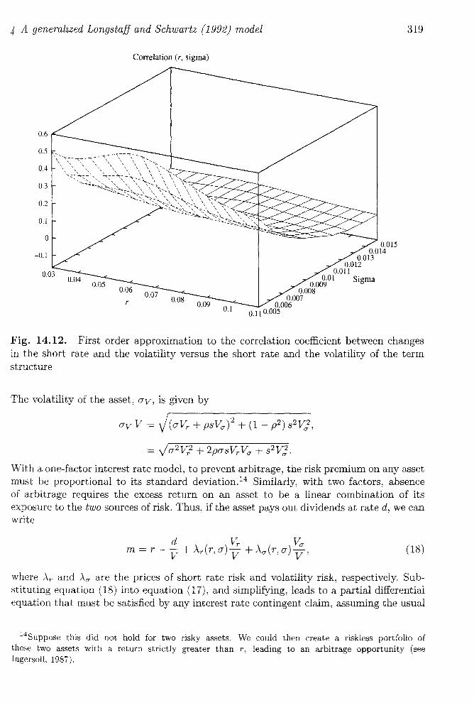
Fig. 14.12. First order approximation to the correlation coefficient between changes in the short rate and the volatility versus the short rate and the volatility of the term structure

The volatility of the asset, O"v, is given by

O"v V = V(O"Vr + pSVa)2 + (1 - p2) s2V;,

= V0"2V? + 2pO"sVrVa + S2V;.

vVith a one-factor interest rate model, to prevent arbitrage, the risk premium on any asset must be proportional to its standard deviation. 14 Similarly, with two factors, absence of arbitrage requires the excess return on an asset to be a linear combination of its exposure to the two sources of risk. Thus, if the asset pays out dividends at rate d, we can write

(18)

where Ar and Aa are the prices of short rate risk and volatility risk, respectively. Sub­stituting equation (18) into equation (17), and simplifying, leads to a partial differential equation that must be satisfied by any interest rate contingent claim, assuming the usual

14Suppose this did not hold for two risky assets. We could then create a riskless portfolio of these two assets with a return strictly greater than T, leading to an arbitrage opportunity (see IngersolL 1987).

320 A multifactor, nonlinear, continuous-time model of interest rate volatility

technical smoothness and integrability conditions (see, for example, Duffie, 1988),

(19)

subject to appropriate boundary conditions. To price interest rate dependent assets, we need to know not only the processes governing movements in rand (7, but also the prices of risk, ,\. and Aa-.

Equation (18) gives an expression for these functions in terms of the partial deriva­tives Vr and Va-, which could be used to estimate the prices of risk, given estimates of these derivatives for two different assets, plus estimates of the excess return for each asset. As mentioned above, it is difficult to estimate derivatives precisely using nonpara­metric density estimation. Therefore, instead of following this route, one could avoid directly estimating the partial derivatives, Vr and Va-, by considering the instantaneous covariances between the asset return and changes in the interest rate/volatility, CVr and eVa-. From equations (14), (15) and (16) (after a little simplification),

(cvr ) _ (dV dr /V dt) ( (72 eVa- = dV d(7 /V dt = P(7S

This can be inverted, as long as [p[ < 1, to obtain

P(7S) -1 (ev r ) s2 eVa-'

1 (1/ (72

1 - p2 -p/(7S -P/(7S) (ev r ) 1/s2 eVa-'

(20)

To preclude arbitrage, the excess return on the asset must also be expressible as a linear combination of eVr and eVa-,

m = r - ~ + A * r(r, (7)eVr + A* a-(r, (7)eva-. (21)

Given two different interest rate dependent assets, we can estimate the instantaneous covariances for each in the same way as we estimated p(r, (7) above. We can also estimate the excess return for each asset, mi(r, (7) - r as a function of the two state variables. The two excess returns can be expressed in the form

which can be inverted to yield an estimate of the prices of risk,

e~a-) -1 (m1 - r) . eVa- m2 - r

Finally, for estimates of the more standard representation of the prices of risk, Ar and /\0") equate equations (18) and (21), using equation (20), to obtain

pm,) (A*r) 2 \ * .

S /\ a-

latility

(19)

;ts, we prices

ieriva­Ltes of reach 1para-avoid

meous TT' and

(20)

linear

(21 )

neous imate .. The

, and

5 Conclusion 321

Given estimates for the process governing movements in rand 0', and the above procedure for the functions AT' and A(7, we can value interest rate dependent assets in one of two ways. The first is to solve equation (19) numerically using a method such as the Hopscotch method of Gourlay and McKee (1977). The second is to use the fact that we can write the solution to equation (19) in the form of an expectation. Specifically, we can write V, the value of an asset which pays out cash flows at a (possibly path-dependent) rate Ct , in the form

v, = E [iT e- J:(f.l dUG, ds 1 ' where i follows the "risk adjusted" process,

for all T > t, and where

(22)

(23)

This says that the value of the asset equals the expected sum of discounted cash flows paid over the life of the asset, except that it substitutes the risk adjusted process (i,0') for the true process (r,o-).

This representation leads directly to a valuation algorithm based on Monte Carlo simulation. For a given starting value of (rt, O't), simulate a number of paths for i and 0' using equations (23) and (24). Along each path, calculate the cash flows Ct , and discount these back along the path followed by the instantaneous riskless rate, it. The average of the sum of these values taken over all simulated paths is an approximation to the expectation in equation (22), and hence to the security value, Vi. The more paths simulated, the closer the approximation.

5. Conclusion

This chapter provides a method for estimating multifactor continuous-time Markov processes. Using Milshtein's (1978) approximation schemes for writing expectations of functions of the sample path of stochastic differential equations in terms of the drift, volatility and correlation coefficients, we provide nonparametric estimation of the drift and diffusion functions of multivariate stochastic differential equations. We apply this technique to the short- and long-end of the term structure for a general two-factor, continuous-time diffusion process for interest rates. In estimating this process, several results emerge. First, the volatility of interest rates is increasing in the level of interest rates, only for sharply, upward sloping term structures. Thus, the result of previous stud­ies, suggesting an almost exponential relation between interest rate volatility and levels, is due to the term structure on average being upward sloping, and is not a general result per se. Second. the finding that partly motivates this chapter, i.e., the link between slope

322 A multifactor, nonlinear, continuous-time model of interest rate volatility

and interest rate volatility in Engle, Lilien and Robins (1987), comes out quite naturally from the estimation. Finally, the slope of the term structure, on its own, plays a large role in determining the magnitude of the diffusion coefficient. These volatility results hold across maturities, which suggests that a low dimensional system (with nonlinear effects) may be enough to explain the term structure of interest rates.

As a final comment, there are several advantages of the procedure adopted in this chapter. First, there is a constant debate between researchers on the relative benefits of using equilibrium versus arbitrage-free models. Here, we circumvent this issue by using actual data to give us the process and corresponding prices of risk. As the real world coincides with the intersection of equilibrium and arbitrage-free models, our model is automatically consistent. Of course, in a small sample, statistical error will produce estimated functional forms that do not conform. This problem, however, is true of all empirical work. Second, we show how our procedure for estimating the underlying multi­factor continuous-time diffusion process can be used to generate fixed income pricing. As an example, we show how our results can be interpreted within a generalized Longstaff and Schwartz (1992) framework, that is, one in which the drift and diffusion coefficients of the instantaneous interest rate and volatility are both (nonlinear) functions of the level of interest rates and the volatility. Third, and perhaps most important, the pricing of fixed-income derivatives depends crucially on the level of volatility. The results in this chapter suggest that volatility depends on both the level and slope of the term structure, and therefore contains insights into the eventual pricing of derivatives.