Embed Size (px)
Citation preview
Linkoping Studies in Science and TechnologyDissertation No. 1171
A Multidimensional Filtering Frameworkwith Applications to Local Structure Analysis
and Image Enhancement
Bjorn Svensson
Department of Biomedical EngineeringLinkopings universitet
SE-581 85 Linkoping, Swedenhttp://www.imt.liu.se
Linkoping, April 2008

A Multidimensional Filtering Frameworkwith Applications to Local Structure Analysis and Image Enhancement
c© 2008 Bjorn Svensson
Department of Biomedical EngineeringLinkopings universitet
SE-581 85 Linkoping, Sweden
ISBN 978-91-7393-943-0 ISSN 0345-7524
Printed in Linkoping, Sweden by LiU-Tryck 2008
Abstract
Filtering is a fundamental operation in image science in general and in medicalimage science in particular. The most central applications are image enhancement,registration, segmentation and feature extraction. Even though these applicationsinvolve non-linear processing a majority of the methodologies available rely oninitial estimates using linear filters. Linear filtering is a well established corner-stone of signal processing, which is reflected by the overwhelming amount ofliterature on finite impulse response filters and their design.
Standard techniques for multidimensional filtering are computationally intense.This leads to either a long computation time or a performance loss caused byapproximations made in order to increase the computational efficiency. This dis-sertation presents a framework for realization of efficient multidimensional filters.A weighted least squares design criterion ensures preservation of the performanceand the two techniques calledfilter networksandsub-filter sequencessignificantlyreduce the computational demand.
A filter network is a realization of a set of filters, which are decomposed into astructure of sparse sub-filters each with a low number of coefficients. Sparsityis here a key property to reduce the number of floating point operations requiredfor filtering. Also, the network structure is important for efficiency, since it deter-mines how the sub-filters contribute to several output nodes, allowing reductionor elimination of redundant computations.
Filter networks, which is the main contribution of this dissertation, has many po-tential applications. The primary target of the research presented here has beenlocal structure analysis and image enhancement. A filter network realization forlocal structure analysis in3D shows a computational gain, in terms of multiplica-tions required, which can exceed a factor70 compared to standard convolution.For comparison, this filter network requires approximately the same amount ofmultiplications per signal sample as a single2D filter. These results are purely al-gorithmic and are not in conflict with the use of hardware acceleration techniquessuch as parallel processing or graphics processing units (GPU). To get a flavor ofthe computation time required, a prototype implementation which makes use offilter networks carries out image enhancement in3D, involving the computationof 16 filter responses, at an approximate speed of1MVoxel/s on a standard PC.

PopularvetenskapligSammanfattning
Filtrering ar en av de mest grundlaggande operationerna inom bildanalys. Dettagaller sarkilt for analys av medicinska bilder, dar bildforbattring, geometrisk bild-anpassning, segmentering och sardragsextraktionar centrala tillampningar. Dessatill ampningar kraver i allmanhet icke-linjar filterering, men de flesta metoder somfinns byggeranda pa berakningar som har sin grund i linjar filtrering. Sedan enlang tid tillbakaar en av grundstenarna i signalbehandling linjara filter och dessdesign.
Standardmetoder for multidimensionell filtrering ar dock i allmanhetberakningsintensiva, vilket resulterar i antingen langa exekveringstider ellersamre prestanda pa grund av de forenklingar som maste goras for att minskaberakningskomplexiteten. Den har avhandlingen presenterar ett ramverk for re-alisering av multidimensionella filter, dar ett minsta-kvadrat kriterium sakerstallerprestanda och de tva teknikerna filternat och filtersekvenser anvands for attavsevart minska berakningskomplexiteten.
Ett filternat ar en realisering av ett flertal filter, som delas upp i en struktur av glesadelfilter med fa koefficienter. Gleshetenar en av de viktigaste egenskaperna for attminska antalet flyttalsoperationer som kravs for filtrering. Natverksstrukturenarocksa viktig for hogre effektivitet, eftersom varje delfilter da samtidigt kan bidratill flera filter och darmed reducera eller eliminera redundanta berakningar.
Det viktigaste bidraget i avhandlingenar filternaten, en teknik som kan tillampasi manga sammanhang. Har anvands den framst till analys av lokal struktur ochbildforbattring. En realisering med filternat for estimering av lokal struktur i3D kan utforas med en faktor70 ganger farre multiplikationer jamfort med falt-ning. Detta motsvarar ungefar samma mangd multiplikationer per sampel somfor ett enda vanligt2D filter. Eftersom filternat enbartar en algoritmisk teknik,finns det ingen motsattning mellan anvandning av filternat och acceleration medhjalp av hardvara, som till exempel parallella berakningar eller grafikkortspro-cessorer. En prototyp har implementerats for filternatsbaserad bildforbattring av3D-bilder, dar 16 filtersvar beraknas. Med denna prototyp utfors bildforbattring ien hastighet av ungefar1MVoxel/s pa en vanlig PC, vilket ger en uppfattning omde berakningstider som kravs for den har typen av operationer.


Acknowledgements
I would like to express my deepest gratitude to a large number of people, who indifferent ways have supported me along this journey.
I would like to thank my main supervisor, Professor Hans Knutsson, for all theadvice during the past years, but also for giving me the opportunity to work in hisresearch group, a creative environment dedicated to research. You have been aconstant source of inspiration and new ideas.
My co-supervisor, Dr. Mats Andersson, recently called me his most hopeless PhDstudent ever, referring to my lack of interest in motor cycles. Nevertheless, wehave had a countless number of informal conversations, which have clarified mythinking. Your help has been invaluable and very much appreciated.
My other co-supervisor, Associate Professor Oleg Burdakov, has taught me basi-cally everything I know about non-linear optimization. Several late evenings ofjoint efforts were spent on improving optimization algorithms.
I would like to thank ContextVision AB for taking an active part in my researchand in particular for the support during a few months to secure the financial sit-uation. The input from past and present members of the project reference group,providing both an industrial and a clinical perspective, has been very important.
All friends and colleagues at the department of Biomedical Engineering, espe-cially the Medical Informatics group and in particular my fellow PhD students inthe image processing group for a great time both on and off work.
All friends from my time in Gothenburg and all friends in Linkoping, includingthe UCPA ski party of 2007 and my floorball team mates. You have kept my mindbusy with more important things than filters and tensors.
My family, thank you for all encouraging words and for believing in me.
Kristin, you will always be my greatest discovery.
The financial support from the Swedish Governmental Agency for Innovation Sys-tems (VINNOVA), the Swedish Foundation for Strategic Research (SSF), Con-textVision AB, the Center for Medical Image Science and Visualization (CMIV)and the Similar Network of Excellence is gratefully acknowledged.

Table of Contents
1 Introduction 11.1 Motivations . . . . . . . . . . . . . . . . . . . . . . . . . . . . . 11.2 Dissertation Outline . . . . . . . . . . . . . . . . . . . . . . . . . 21.3 Contributions . . . . . . . . . . . . . . . . . . . . . . . . . . . . 31.4 List of Publications . . . . . . . . . . . . . . . . . . . . . . . . . 41.5 Abbreviations . . . . . . . . . . . . . . . . . . . . . . . . . . . . 51.6 Mathematical Notation . . . . . . . . . . . . . . . . . . . . . . . 6
2 Local Phase, Orientation and Structure 72.1 Introduction . . . . . . . . . . . . . . . . . . . . . . . . . . . . . 72.2 Local Phase in 1D . . . . . . . . . . . . . . . . . . . . . . . . . . 82.3 Orientation . . . . . . . . . . . . . . . . . . . . . . . . . . . . . 102.4 Phase in Higher Dimension . . . . . . . . . . . . . . . . . . . . . 122.5 Combining Phase and Orientation . . . . . . . . . . . . . . . . . 142.6 Hilbert and Riesz Transforms . . . . . . . . . . . . . . . . . . . . 162.7 Filters Sets for Local Structure Analysis . . . . . . . . . . . . . . 182.8 Discussion . . . . . . . . . . . . . . . . . . . . . . . . . . . . . . 19
3 Non-Cartesian Local Structure 213.1 Introduction . . . . . . . . . . . . . . . . . . . . . . . . . . . . . 213.2 Tensor Transformations . . . . . . . . . . . . . . . . . . . . . . . 223.3 Local Structure and Orientation . . . . . . . . . . . . . . . . . . . 243.4 Tensor Estimation . . . . . . . . . . . . . . . . . . . . . . . . . . 273.5 Discussion . . . . . . . . . . . . . . . . . . . . . . . . . . . . . . 29
4 Tensor-Driven Noise Reduction and Enhancement 314.1 Introduction . . . . . . . . . . . . . . . . . . . . . . . . . . . . . 314.2 Noise Reduction . . . . . . . . . . . . . . . . . . . . . . . . . . . 33
4.2.1 Transform-Based Methods . . . . . . . . . . . . . . . . . 344.2.2 PDE-Based Methods . . . . . . . . . . . . . . . . . . . . 35
4.3 Adaptive Anisotropic Filtering . . . . . . . . . . . . . . . . . . . 384.3.1 Local Structure Analysis . . . . . . . . . . . . . . . . . . 394.3.2 Tensor Processing . . . . . . . . . . . . . . . . . . . . . 404.3.3 Reconstruction and Filter Synthesis . . . . . . . . . . . . 41
4.4 Discussion . . . . . . . . . . . . . . . . . . . . . . . . . . . . . . 42
5 FIR Filter Design 45
viii Table of Contents
5.1 Introduction . . . . . . . . . . . . . . . . . . . . . . . . . . . . . 455.2 FIR Filters . . . . . . . . . . . . . . . . . . . . . . . . . . . . . . 475.3 Weighted Least Squares Design . . . . . . . . . . . . . . . . . . 485.4 Implementation . . . . . . . . . . . . . . . . . . . . . . . . . . . 535.5 Experiments . . . . . . . . . . . . . . . . . . . . . . . . . . . . . 545.6 Discussion . . . . . . . . . . . . . . . . . . . . . . . . . . . . . . 56
6 Sub-Filter Sequences 576.1 Introduction . . . . . . . . . . . . . . . . . . . . . . . . . . . . . 576.2 Sequential Convolution . . . . . . . . . . . . . . . . . . . . . . . 586.3 Multi-linear Least Squares Design . . . . . . . . . . . . . . . . . 59
6.3.1 Alternating Least Squares . . . . . . . . . . . . . . . . . 626.4 Generating Robust Initial Points . . . . . . . . . . . . . . . . . . 62
6.4.1 Implementation . . . . . . . . . . . . . . . . . . . . . . . 656.5 Experiments . . . . . . . . . . . . . . . . . . . . . . . . . . . . . 676.6 Discussion . . . . . . . . . . . . . . . . . . . . . . . . . . . . . . 67
7 Filter Networks 697.1 Introduction . . . . . . . . . . . . . . . . . . . . . . . . . . . . . 697.2 Graph Representation . . . . . . . . . . . . . . . . . . . . . . . . 717.3 Network Structure and Sparsity . . . . . . . . . . . . . . . . . . . 737.4 Least Squares Filter Network Design . . . . . . . . . . . . . . . . 767.5 Implementation . . . . . . . . . . . . . . . . . . . . . . . . . . . 777.6 Experiments . . . . . . . . . . . . . . . . . . . . . . . . . . . . . 797.7 Discussion . . . . . . . . . . . . . . . . . . . . . . . . . . . . . . 81
8 Review of Papers 838.1 Paper I: On Geometric Transformations of Local Structure Tensors 838.2 Paper II: Estimation of Non-Cartesian Local Structure Tensor Fields 838.3 Paper III: Efficient 3-D Adaptive Filtering for Medical Image En-
hancement . . . . . . . . . . . . . . . . . . . . . . . . . . . . . . 848.4 Paper IV: Approximate Spectral Factorization for Design of Effi-
cient Sub-Filter Sequences . . . . . . . . . . . . . . . . . . . . . 848.5 Paper V: Filter Networks for Efficient Estimation of Local 3-D
Structure . . . . . . . . . . . . . . . . . . . . . . . . . . . . . . . 848.6 Paper VI: A Graph Representation of Filter Networks . . . . . . . 85
9 Summary and Outlook 879.1 Future Research . . . . . . . . . . . . . . . . . . . . . . . . . . . 87
1Introduction
The theory and methods presented in this dissertation are results from the tworesearch projectsEfficient Convolution Operators for Image Processing of Vol-umes and Volume SequencesandA New Clinical Quality Level for Medical ImageVolumes. The goal of both these projects have been to develop techniques in forhigh speed filtering of multidimensional signals in high quality medical imageenhancement applications.
1.1 Motivations
This dissertation mainly concerns high speed processing, with particular empha-sis on analysis of local phase, orientation and image structure. This versatile setof features can be utilized for image enhancement, i.e. simultaneous suppressionof high frequency noise and enhancement of minute structures. Similar to themajority of signal processing tools, computation of these features involve the ap-plication of a set of linear filters to the signal.
In general, annD filter is an operator which is applied to a small signal neighbor-hood. In the simplest case the size,Nn, of this neighborhood defines the numberof multiplications required per signal sample, i.e. filtering a volumetric image ofsize512×512×512 voxels with a typical neighborhood size of11×11×11 willrequire1.8 · 1011 multiplications. A corresponding2D filter applied to consecu-tive slices of this volume will have a neighborhood size11 × 11. The number ofmultiplications required is then reduced by a factor11.
Computed tomography and magnetic resonance imaging are two examples usedin clinical routine, which involves processing of multidimensional signals. Eventhough these signals in general have more than2 dimensions, filtering is tradi-tionally carried out in2D. The major reason for limiting the filtering to2D is theincrease of computation time for multidimensional filtering.
Limiting filtering of annD signal to less thann dimensions is however subop-
2 Chapter 1. Introduction
timal since the additional information provided when exploiting all dimensionsavailable improves the signal-to-noise-ratio and enables a better suppression ofhigh-frequency noise. Exploiting the full signal dimensionality also improves theability to more accurately discriminate between signal and noise, which decreasesthe risk of introducing artifacts during filtering and increases the ability of en-hancing minute structures.
In image science in general, there is often a trade-off between performance andspeed. This dissertation primarily targets applications where a more accurate re-sult is desirable, but the computational resources are not sufficient to meet thedemands on computation time. Its usefulness is restricted to methods which relyon linear filters. Even though this dissertation primarily concerns filter sets forlocal structure analysis the presented theory and methods for least squares designof sub-filter sequences and filter networks is applicable for efficient realization ofarbitrary sets of linear filters.
In medical image science, efficient filtering can help to lower the radiation dose incomputed tomography with maintained image quality or alternatively increase theimage quality with the radiation dose unaltered. In magnetic resonance imaging(MRI), it is desirable to prevent artifacts caused by patient movement by having ashort acquisition time. Similar to computed tomography there is in MRI a trade-off between acquisition time and image quality, for which efficient filtering canbe very useful.
1.2 Dissertation Outline
The dissertation consists of two parts, the first part (chapter 2 - 9) provides anoverview of the published papers and some complementary material to the papersincluded in the second part.
Chapter 2 gives an introduction to the concepts local phase, orientation and struc-ture. This leads to a set of filters which are used to estimate these features.
Chapter 3 shows how to take into account the underlying geometry when de-scribing local structure in non-Cartesian coordinate systems.
Chapter 4 primarily concerns adaptive filtering, a method for noise suppressionwhere the concept of local structure is central. Adaptive filtering is also an idealexample of where filter networks is very useful for fast computation.
Chapter 5 describes how operators such as those derived in chapter 2 can be real-ized with finite impulse response filters by solving a linear least squares problem.
Chapter 6 treats the multi-linear least squares problem, which originates from amore efficient filter realization, where a sequence of sparse sub-filters is used.

1.3 Contributions 3
Chapter 7 presents filter networks as a means to significantly lower the compu-tation time for multidimensional filtering and the design problem associated withthis technique.
Chapter 8 briefly reviews the papers included in the dissertation.
Chapter 9 discusses possibilities for future research.
1.3 Contributions
Chapter 2 relies heavily on the work of others, in particular (Knutsson, 1989;Felsberg, 2002). The contribution here is the different viewpoint from which lo-cal phase, orientation and structure is presented. It is shown that the metric ofdifferent vector representations of local phase and orientation leads to a numberof known varieties of local structure tensors.
The summary of Paper I and II in chapter 3 shows how to take into account theunderlying geometry when describing local structure in non-Cartesian coordinatesystems. Steps in this direction have been taken before (Andersson and Knutsson,2003). The primary contribution here is the use of differential geometry to ensurea correct transformation behavior. These theoretic results are also exemplified byexperiments on synthetic data (Paper II) and real data (Paper I).
Chapter 4 presents adaptive filtering (Knutsson et al., 1983; Haglund, 1992) andrelated methodologies for noise suppression. Since adaptive filtering in3D isburdened by a large computational load, the use of filter networks in (Paper III) isan important improvement to this technique.
The least squares framework for filter design in chapter 5 serves as a backgroundto the subsequent two chapters. This chapter is to a large extent based on thework by (Knutsson et al., 1999). However, the experiments and details on theimplementation are original work of the author, which demonstrate some newaspects of this framework.
The contribution of chapter 6 and paper IV is the formulation and implementa-tion of the two-stage approach presented to solve the multi-linear least squaresproblem originating from design of sub-filter sequences.
Least squares design of filter networks was first proposed in (Andersson et al.,1999). The work presented in Paper V, VI and chapter 7, producing3D filtersets, is a generalization of these2D results. Several improvements to the originaloptimization strategy has been made, allowing constraints on the sub-filters withan improved convergence and significantly fewer design variables as a results. Incontrast to Andersson et al. (1999), this technique lends itself to optimization offilter networks producing4D filter sets on a standard PC.
4 Chapter 1. Introduction
1.4 List of Publications
This dissertation is based on six papers, where the author has contributed to ideas,experiments, illustrations and writing. The contributions amount to at least half ofthe total work for every case. The papers appear in the order that best matches thedissertation outline and will be referred to in the text by their Roman numerals.
I. Bjorn Svensson, Anders Brun, Mats Andersson and Hans Knutsson.OnGeometric Transformations of Local Structure Tensors. In manuscript forjournal submission.
II. Bj orn Svensson, Anders Brun, Mats Andersson and Hans Knutsson.Esti-mation of Non-Cartesian Local Structure Tensor Fields. Scandinavian Con-ference on Image Analysis (SCIA). Aalborg, Denmark. 2007.
III. Bj orn Svensson, Mats Andersson,Orjan Smedby and Hans Knutsson.Ef-ficient 3-D Adaptive Filtering for Medical Image Enhancement. IEEE In-ternational Symposium on Biomedical Imaging (ISBI). Arlington, USA.2006.
IV. Bj orn Svensson, Oleg Burdakov, Mats Andersson and Hans Knutsson.Approximate Spectral Factorization for Design of Efficient Sub-FilterSequences. Submitted manuscript for journal publication.
V. Bjorn Svensson, Mats Andersson and Hans Knutsson.Filter Networks forEfficient Estimation of Local 3-D Structure. IEEE International Conferenceon Image Processing (ICIP). Genoa, Italy. 2005.
VI. Bj orn Svensson, Mats Andersson and Hans Knutsson.A Graph Repre-sentation of Filter Networks. Scandinavian Conference on Image Analysis(SCIA). Joensuu, Finland. 2005.
The following publications are related to the material presented but are not in-cluded in the dissertation.
• Bjorn Svensson, Mats Andersson and Hans Knutsson.On Phase-InvariantStructure Tensors and Local Image Metrics. SSBA Symposium on ImageAnalysis. Lund, Sweden. 2008.
• Anders Brun, Bjorn Svensson, Carl-Fredrik Westin, Magnus Herberthson,Andreas Wrangsjo and Hans Knutsson.Using Importance Sampling forBayesian Feature Space Filtering. Scandinavian conference on image anal-ysis(SCIA). Aalborg, Denmark. 2007.
• Bjorn Svensson, Oleg Burdakov, Mats Andersson and Hans Knutsson.ANew Approach for Treating Multiple Extremal Points in Multi-Linear LeastSquares Filter Design. SSBA Symposium on Image Analysis. Linkoping,Sweden. 2007.
1.5 Abbreviations 5
• Bjorn Svensson.Fast Multi-dimensional Filter Networks. Design, Opti-mization and Implementation. Licentiate Thesis1. 2006.
• Bjorn Svensson, Mats Andersson,Orjan Smedby and Hans Knutsson.Radiation Dose Reduction by Efficient 3D Image Restoration. EuropeanCongress of Radiology (ECR). Vienna, Austria. 2006.
• Bjorn Svensson, Mats Andersson and Hans Knutsson.Sparse Approxima-tion for FIR Filter Design. SSBA Symposium on Image Analysis. Umea,Sweden. 2006.
• Max Langer, Bjorn Svensson, Anders Brun, Mats Andersson, HansKnutsson. Design of Fast Multidimensional Filters Using Genetic Al-gorithms. European Workshop on Evolutionary Computing in ImageAnalysis and Signal Processing (EvoIASP). Lausanne, Switzerland. 2005.
• Bjorn Svensson, Mats Andersson, Johan Wiklund and Hans Knutsson.Is-sues on Filter Networks for Efficient Convolution. SSBA Symposium onImage Analysis. Uppsala, Sweden. 2004.
1.5 Abbreviations
Abbreviations used in this dissertation are listed below.
ALS Alternating Least SquaresCT Computed TomographyFFT Fast Fourier TransformFIR Finite Impulse ResponseIFIR Interpolated Finite Impulse ResponseIIR Infinite Impulse ResponseMRI Magnetic Resonance ImagingSNR Signal-to-Noise RatioSVD Singular Value Decomposition
1The licentiate degree is an intermediate degree between master and doctor.

6 Chapter 1. Introduction
1.6 Mathematical Notation
The mathematical notation used for (chapter 2 - 9) is given below. Note that thenotation in the included papers may be slightly different.
v Non-scalar variableI The identity matrixA† Pseudo inverse ofAAT Transpose ofAA∗ Conjugate transpose ofA
ıı Imaginary unitR The set of all real numbersC The set of all complex numbersZ The set of all integersU The set of frequenciesU = u ∈ R
n : |ui| ≤ πN Signal neighborhoodF The Fourier transformH The Hilbert transformR The Riesz transformE
[·]
Expectation of a random variable〈·, ·〉 Inner productu ⊗ v Tensor productu v Element-wise product‖ · ‖ Weightedl2 norm‖ · ‖p Weightedlp normξ ∈ N Spatio-temporal coordinate vectoru ∈ U Frequency coordinate vectorg The metric tensorT The local structure tensor

2Local Phase, Orientation and
Structure
This chapter introduces the concepts of local phase, orientation and structure,which are central for Paper I, II, III and V. Using vector representations, prop-erties of local phase and orientation are here reviewed. Analysis of the metricon the manifolds, defined by these representations, leads to known operators forestimating local structure, i.e. an alternative perspective on local structure tensorsis provided.
2.1 Introduction
Applying local operators for analysis of image structure has been studied for over40 years, see e.g. (Roberts, 1965; Granlund, 1978; Knutsson, 1982; Koenderink,1984; Canny, 1986). The predominant approach is to apply a linear filter or com-bining the responses from a set of linear filters to form a local operator whichdescribes a local image characteristic referred to as an image feature. Alternativeapproaches have appeared more recently in (Felsberg and Jonsson, 2005; Broxet al., 2006), where non-linear operators are used and in (Larkin et al., 2001; Pat-tichis and Bovik, 2007) where non-local operators are used. This dissertation doeshowever only concern local operators, where estimation is performed by combin-ing the responses from a set of linear filters.
In 1D it is customary to decompose a signal into phase and amplitude using shortterm Fourier transforms or filter banks (Gabor, 1946; Allen and Rabiner, 1977).One such decomposition is called the analytic signal and is computed using theHilbert transform. It is either implemented using a complex-valued linear fil-ter or by two real-valued linear filters, from which a vector representation isformed. Essentially the same ideas have later been employed in higher dimen-sions (Granlund, 1978; Daugman, 1980; Maclennan, 1981; Knutsson, 1982) eventhough the extension of the phase concept is not obvious. One extension of theanalytic signal is called the monogenic signal (Felsberg and Sommer, 2001), avector representation which is computed using the Riesz transform.
8 Chapter 2. Local Phase, Orientation and Structure
Also, second order forms have been used for analysis of image structure,e.g. detection of circular features (Forstner and Gulch, 1987), corners (Harrisand Stephens, 1988) and orientation (Bigun and Granlund, 1987; Knutsson,1987). In particular, the concept of orientation has been well studied and formalrequirements for a representation of orientation were derived in (Knutsson, 1985),which are:
The uniqueness requirement:The representation must be unique, i.e. anytwo signal neighborhoods with the same orientation must be mapped ontothe same point.
The uniform stretch requirement: The representation must preserve theangle metric, i.e. it must be continuous and the representation must changeproportionally to the change of orientation.
The polar separability requirement: The norm of the representation mustbe invariant to rotation of the signal neighborhood.
In addition to these requirements a robust representation of orientation is insensi-tive to phase shifts, a property which led to the development of a phase invarianttensor using quadrature filters (Knutsson and Granlund, 1980; Knutsson, 1989).Since the introduction of the tensor as a representation for image structure, nu-merous varieties of tensors and estimation schemes have been developed. Recentefforts have however brought different approaches closer together (Knutsson andAndersson, 2005; Nordberg and Farneback, 2005; Felsberg and Kothe, 2005). Itis in this spirit this chapter should be read, where local phase, orientation andstructure is presented from a slightly different point of view. This presentationwill frequently make use of the Hilbert transform and the Riesz transform. Thesetransforms are defined in Sec 2.6, where also their relation to derivatives is clari-fied.
2.2 Local Phase in 1D
In communication it is common to encode a message as a narrow-band waveforma(t) modulated by a sinusoid. For best performance, the carrier frequency of thissinusoid is adapted to the channel for which the message is intended. Considerfor instance the real-valued signal
f(t) = a(t) cos(ωt+θ0) = a(t)1
2
(
exp(−ıı(ωt+θ0)
)+exp
(ıı(ωt+θ0)
))
, (2.1)
whereω is the carrier frequency. One way to demodulate the signal is to form theanalytic signalfa defined by
fa(t) = f(t) + ııH(f)(t), (2.2)
whereH is the Hilbert transform. It is the transformation of a real sinusoid, with-out loss of information, to a complex exponential with only positive frequencies.
2.2 Local Phase in 1D 9
Forf(t), the analytic signal corresponds to the second term in (2.1). For general-ization to higher dimension it is convenient to drop the complex numbers and viewthe analytic signal as an embedding of the signalf(t) in a higher-dimensionalspace,fa : R → R
2, i.e. the analytic signal is the vector
fa(t) =(
f(t),H(f)(t))
=(
a(t) cos(ωt+ θ0), a(t) sin(ωt+ θ0))
, (2.3)
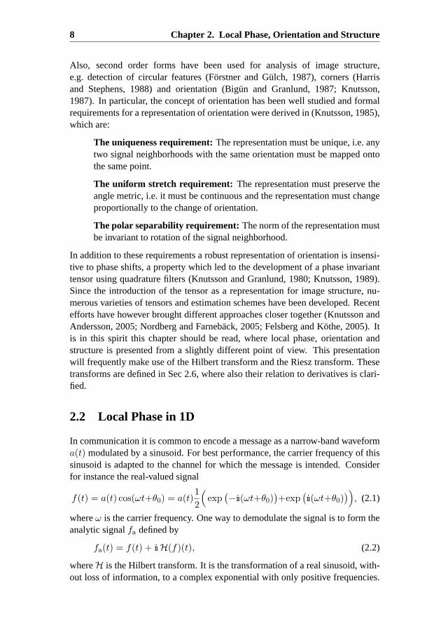
wheref(t) is the in-phase component andH(f)(t) is the quadrature component,which is in quadrature (π2 radians out of phase) with the in-phase component. Thisvector representation of phase can be thought of as a decomposition of even andodd signal energy, which is illustrated in Fig. 2.1. The color-coded phaseis alsoshown for a Gaussian function modulated by a sinusoid.
fa(t)
f
H(f)
θ
0
π2
π
3π2
2π
Figure 2.1: Left: A 1D Gaussian modulated with a carrier frequency.Right: The ana-lytic signal as a vector representation of phase in1D.
The norm of the analytic signal is called the instantaneous amplitude and consti-tutes an estimate of the encoded message ifa(t) > 0 . The argument representsthe instantaneous phase, i.e. the vectorfa can be decomposed as follows:
a(t) = ‖fa(t)‖ =√
f2(t) + H(f)2(t)
θ(t) = arctan(H(f)(t)
f(t)). (2.4)
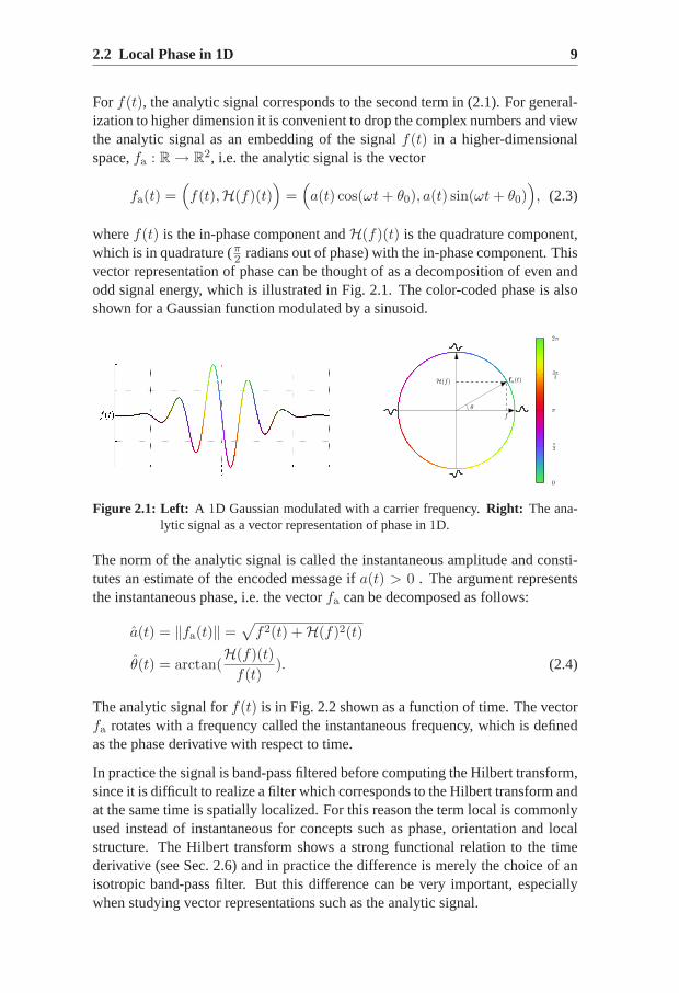
The analytic signal forf(t) is in Fig. 2.2 shown as a function of time. The vectorfa rotates with a frequency called the instantaneous frequency, which is definedas the phase derivative with respect to time.
In practice the signal is band-pass filtered before computing the Hilbert transform,since it is difficult to realize a filter which corresponds to the Hilbert transform andat the same time is spatially localized. For this reason the term local is commonlyused instead of instantaneous for concepts such as phase, orientation and localstructure. The Hilbert transform shows a strong functional relation to thetimederivative (see Sec. 2.6) and in practice the difference is merely the choice of anisotropic band-pass filter. But this difference can be very important, especiallywhen studying vector representations such as the analytic signal.
10 Chapter 2. Local Phase, Orientation and Structure
Figure 2.2: Left: The analytic signal of the1D Gaussian as a function of time.Right:The analytic signal of the1D Gaussian.
Consider the sinusoidf(t) = cos θ(t), which is represented by the analytic signal
fa = (cos θ, sin θ). (2.5)
Comparefa to the vector
r =(
f,df
dt
)
=(
cos θ,−ω sin θ)
. (2.6)
The difference is the factorω = dθdt
which appears in the latter representation.This means that the second element is expressed in per meter as opposed to thefirst one, which is the signal itself. This is because the derivative acts asa high-pass filter, whereas the Hilbert transform preserves the signal spectrum. Repre-sentations which use derivatives of different order (r is here a representation oforder0 and1) often show multi-modal responses, since the derivative alters thesignal spectrum. The Hilbert transform is scale invariant and preserves the phasemetric, which makes it more suitable for vector representations of this kind. Be-fore studying how phase can be generalized to higher dimensions, let us first studythe concept of orientation.
2.3 Orientation
Demodulation of fringe patterns in higher dimensions differs from the1D casein a fundamental way. As opposed to a1-dimensional signal a fringe pattern inhigher dimension has a certain direction. With the same signal model as in theprevious section it is possible to describe a signal of higher dimension by lettingthe phase be a function ofx ∈ R
n, i.e.
f(x) = a(x) cos(θ(x)). (2.7)
This local model is a good approximation of the signal if the phaseθ(x) andamplitude of a signal can be assumed to be slowly varying. For comparison a firstorder Taylor expansion assumes a signal to be locally linear and is well suited to
2.3 Orientation 11
describe signals where the second order derivative can be assumed to be small.Locally, the phase can be described by the linear model as a function of the offset∆x from x
θ(∆x) ≈ θ + 〈∇θ,∆x〉 = θ + ρ〈u,∆x〉, (2.8)
where the local frequency∇θ = ρu now has a direction. The simplest and pos-sibly naive way to represent this new degree of freedom is to use the vectoru
itself. This vector can for instance be estimated using the first order Riesz trans-formR(f). SinceR(f) is a generalization of the Hilbert transform, it inherits thesame relationship to derivatives. The Riesz transform off in (2.7) is
R(f) = a sin θ u (2.9)
and differs from the gradient∇f only1 by the factorρ. These results can be ex-tended to signalsf which are intrinsically1-dimensional. Such functions satisfiesthe simple signal constraintf(x) = f(〈x,v〉v) for some vectorv of unit length(Granlund and Knutsson, 1995). For the sake of simplicity, let us here and hence-forth assume thatf is a sinusoid in2D, i.e. the amplitudea(x) is assumed to beequal to one andu = [cosϕ, sinϕ]T . The Riesz transform then yields a vectorr ∈ R
2, i.e.
r(ϕ) =(
R1(f),R2(f))
= sin θ(
cosϕ, sinϕ)
. (2.10)
This vector is a sufficient representation of orientation for a fixedθ 6= 0, but ifθ varies a few problems occur. The amplitude of the signal, here equal to one,is mixed up with the phase and forθ = 0 the information about orientation islost. Even if these problems are resolved, the representation is not unique sinceidentical signals can appear as antipodal points as seen in Fig. 2.3. An elegantremedy to the latter problem is, in2D, to compute the non-linear combination ofthe elements in (2.10) such that
r(ϕ) = sin2 θ(
cos2 ϕ− sin2 ϕ, 2 sinϕ cosϕ)
, (2.11)
wherer(ϕ) rotates with twice the speed. This is known as the double angle rep-resentation (Granlund, 1978).
Another possibility is to study the metricg on the the manifold defined by (2.10).Since the vector representation is continuous the metric must be the same for twoidentical signals, even if they are mapped to different points. The elements ofg
are given by the partial derivatives ofr with respect tox, i.e.
gij =
[
| ∂r∂x1 |2 ∂r
∂x1 · ∂r∂x2
∂r∂x1 · ∂r
∂x2 | ∂r∂x2 |2
]
= ρ2 cos2 θ
[cos2 ϕ cosϕ sinϕ
cosϕ sinϕ sin2 ϕ
]
. (2.12)
1If a(x) is a narrow-band signal the influence of∇a can be considered as negligible.
12 Chapter 2. Local Phase, Orientation and Structure
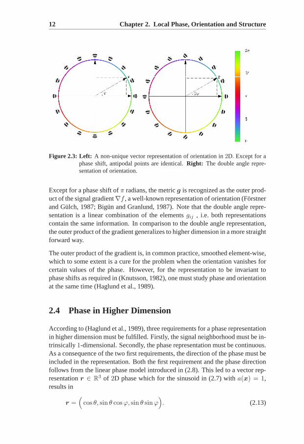
Figure 2.3: Left: A non-unique vector representation of orientation in2D. Except for aphase shift, antipodal points are identical.Right: The double angle repre-sentation of orientation.
Except for a phase shift ofπ radians, the metricg is recognized as the outer prod-uct of the signal gradient∇f , a well-known representation of orientation (Forstnerand Gulch, 1987; Bigun and Granlund, 1987). Note that the double angle repre-sentation is a linear combination of the elementsgij , i.e. both representationscontain the same information. In comparison to the double angle representation,the outer product of the gradient generalizes to higher dimension in a more straightforward way.
The outer product of the gradient is, in common practice, smoothed element-wise,which to some extent is a cure for the problem when the orientation vanishes forcertain values of the phase. However, for the representation to be invariant tophase shifts as required in (Knutsson, 1982), one must study phase and orientationat the same time (Haglund et al., 1989).
2.4 Phase in Higher Dimension
According to (Haglund et al., 1989), three requirements for a phase representationin higher dimension must be fulfilled. Firstly, the signal neighborhood must bein-trinsically1-dimensional. Secondly, the phase representation must be continuous.As a consequence of the two first requirements, the direction of the phasemust beincluded in the representation. Both the first requirement and the phase directionfollows from the linear phase model introduced in (2.8). This led to a vector rep-resentationr ∈ R
3 of 2D phase which for the sinusoid in (2.7) witha(x) = 1,results in
r =(
cos θ, sin θ cosϕ, sin θ sinϕ)
. (2.13)
2.4 Phase in Higher Dimension 13
This generalizes to a representationr ∈ Rn+1 for a multidimensional signal
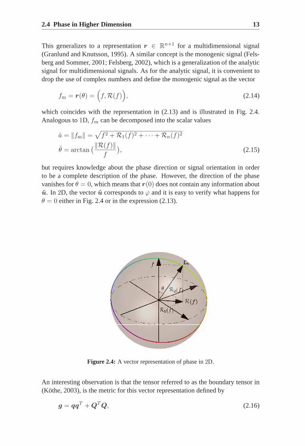
(Granlund and Knutsson, 1995). A similar concept is the monogenic signal(Fels-berg and Sommer, 2001; Felsberg, 2002), which is a generalization of theanalyticsignal for multidimensional signals. As for the analytic signal, it is convenienttodrop the use of complex numbers and define the monogenic signal as the vector
fm = r(θ) =(
f,R(f))
, (2.14)
which coincides with the representation in (2.13) and is illustrated in Fig. 2.4.Analogous to1D, fm can be decomposed into the scalar values
a = ‖fm‖ =√
f2 + R1(f)2 + · · · + Rn(f)2
θ = arctan(‖R(f)‖
f
), (2.15)
but requires knowledge about the phase direction or signal orientation inorderto be a complete description of the phase. However, the direction of the phasevanishes forθ = 0, which means thatr(0) does not contain any information aboutu. In 2D, the vectoru corresponds toϕ and it is easy to verify what happens forθ = 0 either in Fig. 2.4 or in the expression (2.13).
Figure 2.4: A vector representation of phase in2D.
An interesting observation is that the tensor referred to as the boundary tensor in(Kothe, 2003), is the metric for this vector representation defined by
g = qqT + QTQ, (2.16)
14 Chapter 2. Local Phase, Orientation and Structure
where the elementsqi = ρRi(f) andQij = ρRiRj(f) are determined by thefirst and second order Riesz transform. Note that the first term is the outer productof the gradient, which is sensitive for odd signal energies and hence also phasevariant. This will be compensated for, by the second term which captures evensignal energies. For simple signals this leads to the phase invariant local structuretensor with elements
gij = ρ2(sin2 θ + cos2 θ)
[cos2 ϕ cosϕ sinϕ
cosϕ sinϕ sin2 ϕ
]
. (2.17)
A similar construction has been proposed by (Farneback, 2002), where the Hes-sian squared is used. The second termQ used here differs from the Hessianmatrix only by a factorρ, which ensures that the first and the second term ofg arecomputed with respect to the same signal spectrum.
An approach similar to the monogenic signal is the use of loglet filters (Knutssonand Andersson, 2005). In fact the output of a loglet filter of order0 is identicalto the monogenic signal. An individual loglet produces a vector valued filter re-sponse inRn+1. Whereas the monogenic signal is a representation of the phase inthe dominant orientation, a loglet filter of higher order measures the phase with anorientational bias. From a set of loglet filters in different directions it is thereforepossible to synthesize the local phase for an arbitrary orientation. It turns out thatthe elements from such a set can be identified as elements of higher order Riesztransforms or a linear combination of such elements. This indicates that a vec-tor representation using higher order terms might be an approach to resolve theproblem with vanishing information for certain values of the phase.
2.5 Combining Phase and Orientation
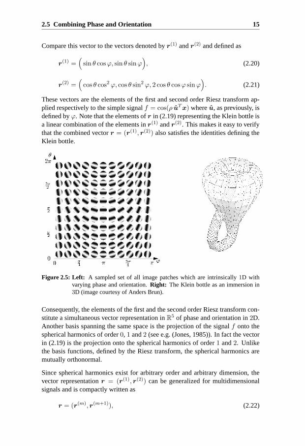
The topological structure of simple signals in2D with arbitrary phase and orien-tation is described by a Klein bottle (Tanaka, 1995; Swindale, 1996), which alsohas been verified experimentally in (Brun et al., 2005; Carlsson et al., 2008). Arepresentation of the Klein bottle must satisfy the following identities
r(ϕ, θ) = r(ϕ, θ + 2π),
r(ϕ, θ) = r(ϕ+ π, 2π − θ), (2.18)
which is also illustrated in Fig. 2.5, where samples of all possibleθ andϕ areshown. A Klein bottle cannot be embedded without self-intersections inR
3,which explains why the information of orientation vanishes in the phase repre-sentation and that simultaneous representation of orientation and phase could notbe accomplished with only3 elements. One possible representation of the Kleinbottle inR
4 is
r =(
sin θ cosϕ, sin θ sinϕ, cos θ(cos2 ϕ−sin2 ϕ), 2 cos θ cosϕ sinϕ)
. (2.19)
2.5 Combining Phase and Orientation 15
Compare this vector to the vectors denoted byr(1) andr(2) and defined as
r(1) =(
sin θ cosϕ, sin θ sinϕ)
, (2.20)
r(2) =(
cos θ cos2 ϕ, cos θ sin2 ϕ, 2 cos θ cosϕ sinϕ)
. (2.21)
These vectors are the elements of the first and second order Riesz transform ap-plied respectively to the simple signalf = cos(ρ uTx) whereu, as previously, isdefined byϕ. Note that the elements ofr in (2.19) representing the Klein bottle isa linear combination of the elements inr(1) andr(2). This makes it easy to verifythat the combined vectorr = (r(1), r(2)) also satisfies the identities defining theKlein bottle.
Figure 2.5: Left: A sampled set of all image patches which are intrinsically1D withvarying phase and orientation.Right: The Klein bottle as an immersion in3D (image courtesy of Anders Brun).
Consequently, the elements of the first and the second order Riesz transform con-stitute a simultaneous vector representation inR
5 of phase and orientation in2D.Another basis spanning the same space is the projection of the signalf onto thespherical harmonics of order0, 1 and2 (see e.g. (Jones, 1985)). In fact the vectorin (2.19) is the projection onto the spherical harmonics of order1 and2. Unlikethe basis functions, defined by the Riesz transform, the spherical harmonics aremutually orthonormal.
Since spherical harmonics exist for arbitrary order and arbitrary dimension, thevector representationr = (r(1), r(2)) can be generalized for multidimensionalsignals and is compactly written as
r = (r(m), r(m+1)), (2.22)

16 Chapter 2. Local Phase, Orientation and Structure
wherer(m) are spherical harmonics of orderm applied to the signalf . Letr(o),r(e) be the odd and even order elements ofr respectively. For the simplesignalf , the metric for this representation is, as previously, derived from the par-tial derivatives
∂r(o)
∂xi= ρ cos θ ui r
(o), (2.23)
∂r(e)
∂xi= −ρ sin θ ui r
(e). (2.24)
These results can be verified by computing the partial derivatives for the2D exam-ples. Another possibility for verifying these results is to use the Riesz transformsince the relation between spherical harmonics and the Riesz transform also gen-eralize to higher dimension. Like in the previous section the metric leads to aphase invariant local structure tensor
g = ρ2(〈r(o), r(o)〉 cos2 θ + 〈r(e), r(e)〉 sin2 θ) u ⊗ u, (2.25)
since the elements ofr(m) are mutually orthonormal, i.e.〈r(m), r(m)〉 = 1. Thederived metric is conceptually very close to the local structure tensor derived inKnutsson and Andersson (2005), which is computed from spherical harmonics oforder0-3. Another idea in the same direction is the use of higher order derivativesor Riesz transforms as proposed in Felsberg and Kothe (2005). This tensor wasderived using Riesz-transforms of order1, 2 and3, which correspond to a filterbasis which spans the same space. But to compute the tensor in (2.25) from sucha basis the appropriate inner product must be used.
2.6 Hilbert and Riesz Transforms
For completeness this section goes into more details on the Hilbert and the Riesztransform and their relation to derivatives. The Hilbert transformH applied to asignalF (u) is in the Fourier domain defined by
H(F )(u) = ıı sign(u)F (u) = ııu
‖u‖F (u). (2.26)
The latter equality is provided to see the connection to the Riesz transform in(2.29). In the spatial domain, the Hilbert transform is computed as the convolu-tion
H(f)(x) =1
π
∫
R
f(ξ)1
ξ − xdξ = h(x) ∗ f(x), (2.27)
where the filter kernelh(x) is given by
h(x) = − 1
πx. (2.28)
2.6 Hilbert and Riesz Transforms 17
A nice generalization of the Hilbert transform ton dimensions is the Riesz trans-form which is a mapping fromRn → R
n. In the Fourier domain its componentsR1, . . .Rn when applied toF (u) are
Ri(F )(u) = ııui‖u‖F (u). (2.29)
In the spatial domain the equivalent formula is the convolution integral
Ri(f)(x) =Γ(n+1
2 )
πn+1
2
∫
Rn
f(ξ)ξi − xi
‖ξ − x‖n+1dξ = hi(x) ∗ f(x). (2.30)
where the filter kernelhi(x) is given by
hi(x) = −c xi
‖x‖n+1. (2.31)
The normalization constantc is defined by the gamma function and for the mostcommon dimensionalitiesn = 2, 3, 4 this constant takes on the scalar valuesc = 1
2π ,1π2 ,
34π2 .
In the Fourier domain it is easy to see the resemblance to derivatives, i.e.Ri(f)differs from the partial derivative
F ∂f∂xi
(x) = ııuiF (u) (2.32)
only by a factor‖u‖. The same property can in the spatial domain be derivedusing integration by parts, i.e. exploiting the convolution property
∂
∂xi(f ∗ g)(x) =
∂
∂xif(x) ∗ g(x) = f(x) ∗ ∂
∂xig(x). (2.33)
Substitutinghi(x) = ∂∂xi g(x) in (2.30) yields
Ri(f) =∂
∂xif(x) ∗ g(x), (2.34)
which results in the convolution kernel
g(x) =c
n− 1
1
‖x‖n−1. (2.35)
To emphasize its relation to derivatives2 the Riesz-transform can be expressed interms of the signal gradient:
R(f)(x) = ∇f(x) ∗ g(x) (2.36)
2The Hilbert transform can in the same way be expressed as the convolutionH(f)(x) =d
dxf(x) ∗ − 1
πlog(‖x‖)
18 Chapter 2. Local Phase, Orientation and Structure
Naturally, the relation to derivatives generalizes to higher order Riesz transforms.A Riesz transform of orderm is a tensor, which is obtained in the spatial domainby a sequence ofm convolutions, i.e.
Ri1 · · ·Rim(f)(x) =∂m
∂xi1 · · · ∂xim f(x) ∗ g(x) ∗ · · · ∗ g(x)︸ ︷︷ ︸
m
. (2.37)
In the Fourier domain the elements of this tensor are defined by
Ri1 . . .Rim(F )(u) = ıımui1 . . . uim‖u‖m F (u), (2.38)
and differ from them:th order derivative by a factor‖u‖m.
In order to compute derivatives and global transforms such as the Hilbert andRiesz transform the effects of sampling must be taken into account. Let us proceedwith some practical considerations concerning the operators used in this chapter.
2.7 Filters Sets for Local Structure Analysis
Estimation of derivatives, Hilbert and Riesz transforms for sampled data is anill-posed problem (Bracewell, 1986). For instance, the computation of the Riesztransform for an arbitrary signal,f , cannot be computed in practice unless the sig-nal is band-limited, since the transfer function is difficult to realize with a digitalfilter. Therefore the signal is typically band-pass filtered, i.e. the Riesz trans-form actually computed isR(f ∗ g)(x), whereg is a band-pass filter, rather thanR(f)(x) which is the desired. This can be seen as regularization and ideally thefilter g should affect the signal as little as possible.
The operators presented in this chapter are formed by linear filters which can beexpressed in the Fourier domain as
H(u) = R(ρ)D(u), (2.39)
whereρ and u are polar coordinates such thatu = ρu. Such filters are calledpolar separable and are composed by a radial functionR(ρ) and a directionalfunctionD(u). The elements of the ideal second order Riesz transform in2D arefor instance computed with the set of filters
H1, H2, H3 = u12
‖u‖2,u1u2
‖u‖2,u2
2
‖u‖2 (2.40)
which corresponds toDk = Hk andRk(ρ) = 1 for k = 1, . . . , 3. The idealsecond order partial derivatives correspond to the same directional functions butwith radial functionsRk(ρ) = ρ2. Since neither of these two filter sets can berealized with digital filters, the difference between them is merely the choice of anisotropic band-pass filterg which defines the radial functionR(ρ) used in practice.

2.8 Discussion 19
The band-pass filter must be chosen carefully since it is critical that the filterfrequency characteristics make the filter set sensitive for the signal content ofinterest. An extensive overview of different band-pass filters used is given in(Boukerroui et al., 2004)3. In this dissertation either lognormal or logerf functionsare used. The lognormal function is well established and has nice properties foranalysis of local frequency (Granlund and Knutsson, 1995), whereas the logerffunction is better suited for multi-scale analysis (Knutsson and Andersson, 2005).
The choice of the directional functions is not critical, as long as the distribution ofthe filter main directions is fairly even. It would, for instance, not make sense toestimate a derivative in2D by applying two filters with main directions separatedonly by a few degrees. The spherical harmonics are evenly distributed and are inthis sense the best choice. However, filter sets with directional functions that arebetter aligned with the discrete spatial grid are easier to realize and therefore leadto digital filters which are closer to the desired operator.
Another choice are the filter orders, which also determine the number of filters inthe filter set. Many of the representations presented in this chapter make use ofa minimum amount of information obtained by, for instance, the first order Riesztransform. Such representations are incapable of detecting deviations from thesignal model. The redundant information obtained by increasing the dimension-ality of the representation enables description of a larger class of signals. Thisinformation can be used to achieve insensitivity to signal phase, which requiresboth odd and even order filters. Detection of deviations from the signal modelis important for certain applications. This can be accomplished by computing adistance measure between the best fit to the signal model and the observed mea-surements. The richer signal model, obtained from increasing the order of thefilters, comes at the expense of a higher computational load since a larger filter setis required. Efficient realization of filter sets using filter networks, to be presented,can compensate for this increase in computational load.
2.8 Discussion
A review of local phase, orientation and structure was presented in this chapterleading to a family of polar separable filters for local structure analysis. Thesefilters are defined in the Fourier domain by their frequency responses. Realizationof digital filters which approximate these desired operators is central in the workto be presented and in particular this family of filters will be frequently used inexamples throughout the dissertation.
The relationship between derivatives and Riesz transforms is not a novel con-
3The filters evaluated in (Boukerroui et al., 2004) are optimized for white noise and no effortto localize the filters was made. Therefore the results are in direct conflict with the results ine.g. (Knutsson and Andersson, 2005)

20 Chapter 2. Local Phase, Orientation and Structure
tribution, but their relation expressed in the spatial domain is not easily foundin signal processing literature. Such relations are useful for signal processingon non-Cartesian domains, irregular domains and surfaces. For such problems,it is very complicated and sometimes even impossible to design local operatorswhich are defined in the Fourier domain. This problem occurs for instance inthe next chapter where local structure analysis is applied to signals acquired innon-Cartesian coordinate systems.
3Non-Cartesian Local Structure
This chapter concerns how to take into account the underlying geometry whendescribing local structure in non-Cartesian coordinate systems. Particular empha-sis is paid to how the tensors transform when altering the coordinate system andhow this affects the operators that are used for estimation. The chapter is a briefsummary of the work presented in Paper I and II, which to a large extent is basedon the same basic principles.
3.1 Introduction
Geometry is very important in medical imaging, where for instance abnormalitiescan be detected by size, shape and location. It is however common that samplesobtained from acquisition are represented in a non-Cartesian coordinate system.Non-cubic voxels are perhaps the most common example, but more complex ge-ometries are also utilized such as oblique sampling or samples acquired in a polarcoordinate system. Signals acquired from such an imaging device are generallyresampled in order to present a geometrically correct image. Computerized anal-ysis of the signal such as localization of objects or estimation of shape and sizedoes not, however, require resampling. In fact, resampling often complicates sub-sequent processing, since signal and noise characteristics are deteriorated. Thisreasoning applies to local structure in particular, since it is a feature which relatesto geometry.
Even though sampling in non-Cartesian coordinate systems are common, analy-sis and processing of local structure tensor fields in such systems is less devel-oped. Previous work on local structure in non-Cartesian coordinate systems in-clude Westin et al. (2000); Ruiz-Alzola et al. (2002); Andersson and Knutsson(2003). The former two are application oriented, while the latter is a step inthe same direction as Paper I and II. In contrast to previous work, the researchpresented here reviews the concept of local structure and orientation using basicdifferential geometry. This is relevant, since most existing theory on this topic
22 Chapter 3. Non-Cartesian Local Structure
implicitly assumes an underlying Cartesian geometry.
The index notation from tensor calculus used in this chapter will be explainedalong the way and hopefully also facilitate the reading of Paper I and II forthoseunfamiliar with this notation. Index notation helps to distinguish between con-travariant and covariant tensors, a property which becomes important when study-ing non-Cartesian tensor fields.
3.2 Tensor Transformations
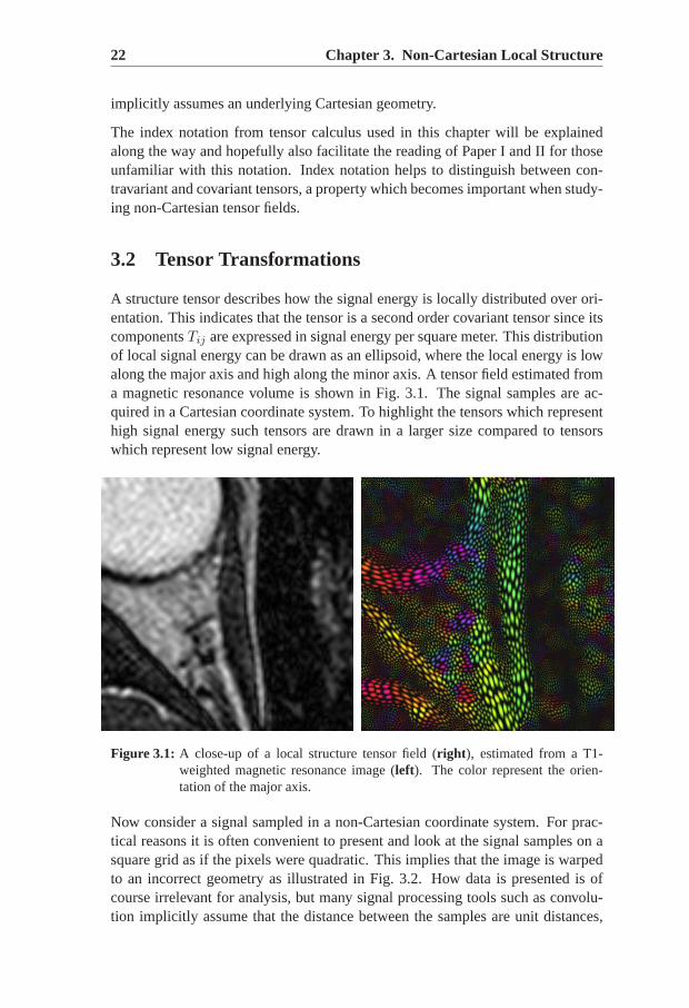
A structure tensor describes how the signal energy is locally distributed over ori-entation. This indicates that the tensor is a second order covariant tensorsince itscomponentsTij are expressed in signal energy per square meter. This distributionof local signal energy can be drawn as an ellipsoid, where the local energy is lowalong the major axis and high along the minor axis. A tensor field estimated froma magnetic resonance volume is shown in Fig. 3.1. The signal samples are ac-quired in a Cartesian coordinate system. To highlight the tensors which representhigh signal energy such tensors are drawn in a larger size compared to tensorswhich represent low signal energy.
Figure 3.1: A close-up of a local structure tensor field (right ), estimated from a T1-weighted magnetic resonance image (left). The color represent the orien-tation of the major axis.
Now consider a signal sampled in a non-Cartesian coordinate system. For prac-tical reasons it is often convenient to present and look at the signal samples on asquare grid as if the pixels were quadratic. This implies that the image is warpedto an incorrect geometry as illustrated in Fig. 3.2. How data is presented is ofcourse irrelevant for analysis, but many signal processing tools suchas convolu-tion implicitly assume that the distance between the samples are unit distances,
3.2 Tensor Transformations 23
i.e. a Cartesian coordinate system. To compensate for the geometric distortion,the spatially varying metric in the warped coordinate system must be taken intoaccount. Let us first study the ideal behavior of local structure tensor if the coor-dinate system is altered.
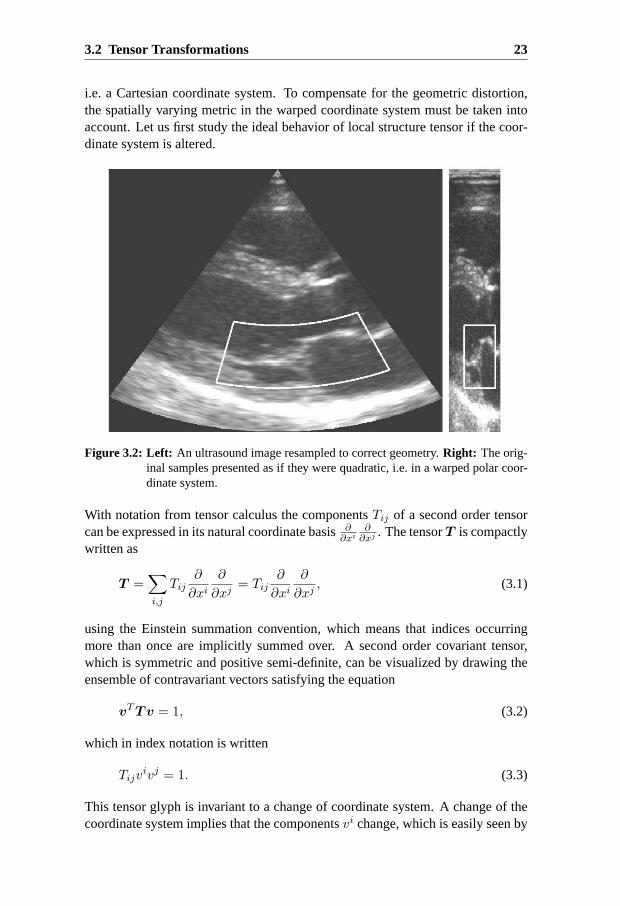
Figure 3.2: Left: An ultrasound image resampled to correct geometry.Right: The orig-inal samples presented as if they were quadratic, i.e. in a warped polar coor-dinate system.
With notation from tensor calculus the componentsTij of a second order tensorcan be expressed in its natural coordinate basis∂
∂xi∂∂xj . The tensorT is compactly
written as
T =∑
i,j
Tij∂
∂xi∂
∂xj= Tij
∂
∂xi∂
∂xj, (3.1)
using the Einstein summation convention, which means that indices occurringmore than once are implicitly summed over. A second order covariant tensor,which is symmetric and positive semi-definite, can be visualized by drawing theensemble of contravariant vectors satisfying the equation
vTTv = 1, (3.2)
which in index notation is written
Tijvivj = 1. (3.3)
This tensor glyph is invariant to a change of coordinate system. A change of thecoordinate system implies that the componentsvi change, which is easily seen by
24 Chapter 3. Non-Cartesian Local Structure
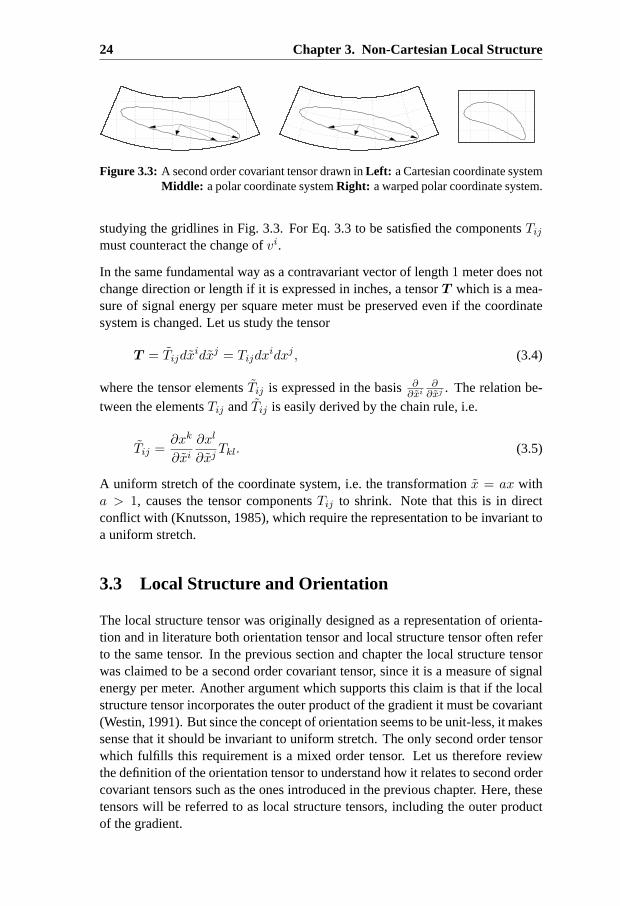
Figure 3.3: A second order covariant tensor drawn inLeft: a Cartesian coordinate systemMiddle: a polar coordinate systemRight: a warped polar coordinate system.
studying the gridlines in Fig. 3.3. For Eq. 3.3 to be satisfied the componentsTijmust counteract the change ofvi.
In the same fundamental way as a contravariant vector of length1 meter does notchange direction or length if it is expressed in inches, a tensorT which is a mea-sure of signal energy per square meter must be preserved even if the coordinatesystem is changed. Let us study the tensor
T = Tijdxidxj = Tijdx
idxj , (3.4)
where the tensor elementsTij is expressed in the basis∂∂xi
∂∂xj . The relation be-
tween the elementsTij andTij is easily derived by the chain rule, i.e.
Tij =∂xk
∂xi∂xl
∂xjTkl. (3.5)
A uniform stretch of the coordinate system, i.e. the transformationx = ax witha > 1, causes the tensor componentsTij to shrink. Note that this is in directconflict with (Knutsson, 1985), which require the representation to be invariant toa uniform stretch.
3.3 Local Structure and Orientation
The local structure tensor was originally designed as a representation of orienta-tion and in literature both orientation tensor and local structure tensor often referto the same tensor. In the previous section and chapter the local structure tensorwas claimed to be a second order covariant tensor, since it is a measure of signalenergy per meter. Another argument which supports this claim is that if the localstructure tensor incorporates the outer product of the gradient it must be covariant(Westin, 1991). But since the concept of orientation seems to be unit-less, it makessense that it should be invariant to uniform stretch. The only second order tensorwhich fulfills this requirement is a mixed order tensor. Let us therefore reviewthe definition of the orientation tensor to understand how it relates to second ordercovariant tensors such as the ones introduced in the previous chapter. Here, thesetensors will be referred to as local structure tensors, including the outer productof the gradient.
3.3 Local Structure and Orientation 25
The orientation tensor is defined only for signalsf which are intrinsically one-dimensional. Such signals satisfy the simple signal constraint
f(x) = f(〈x,v〉v), (3.6)
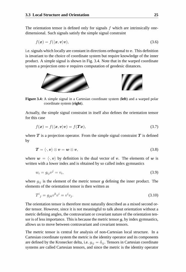
i.e. signals which locally are constant in directions orthogonal tov. This definitionis invariant to the choice of coordinate system but require knowledge of the innerproduct. A simple signal is shown in Fig. 3.4. Note that in the warped coordinatesystem a projection ontov requires computation of geodesic distances.
Figure 3.4: A simple signal in a Cartesian coordinate system (left) and a warped polarcoordinate system (right ).
Actually, the simple signal constraint in itself also defines the orientation tensorfor this case
f(x) = f(〈x,v〉v) = f(Tx), (3.7)
whereT is a projection operator. From the simple signal constraintT is definedby
T = 〈·,v〉 ⊗ v = w ⊗ v, (3.8)
wherew = 〈·,v〉 by definition is the dual vector ofv. The elements ofw iswritten with a lower index and is obtained by so called index gymnastics
wi = gijvj = vi, (3.9)
wheregij is the element of the metric tensorg defining the inner product. Theelements of the orientation tensor is then written as
T ij = gjkvkvi = vivj . (3.10)
The orientation tensor is therefore most naturally described as a mixed second or-der tensor. However, since it is not meaningful to talk about orientation without ametric defining angles, the contravariant or covariant nature of the orientation ten-sor is of less importance. This is because the metric tensorg, by index gymnastics,allows us to move between contravariant and covariant tensors.
The metric tensor is central for analysis of non-Cartesian local structure. In aCartesian coordinate system the metric is the identity operator and its componentsare defined by the Kronecker delta, i.e.gij = δij . Tensors in Cartesian coordinatesystems are called Cartesian tensors, and since the metric is the identity operator
26 Chapter 3. Non-Cartesian Local Structure
there is no need to distinguish between contravariant and covariant tensors. Themetric tensorg defines the inner product
〈u,v〉 = uTg v, (3.11)
whereu, v are contravariant vectors. In index notation the equivalent expressionis written
〈u,v〉 = g(u,v) = gijuivi. (3.12)
In the case of non-cubic voxels, the off-diagonal elements of the metric are zerowhereas the diagonal elements are scaled differently, i.e. the metric is still orthog-onal but not orthonormal. For oblique sampling all elements of the metric arenon-zero. In both these cases the metric is globally defined bygij , which is notthe case for the polar coordinate system wheregij varies with spatial position.With knowledge about the local metric, defining local distances, it is possible toperform analysis of non-Cartesian local structure in the original sampling grid.
Let us for instance study the relation between orientation and local structure. In aCartesian system the dominant signal orientation can be extracted from the localstructure tensor by eigenvalue decomposition, searching for the direction of max-imal detected signal energy. In non-Cartesian coordinate systems this is in thesame way accomplished by finding the vectorv of unit length which maximizes
maxv
vTTv, subject to〈v,v〉 = 1, (3.13)
which in index notation is written as
maxv
Tijvivj , subject togijv
ivj = 1. (3.14)
The metricg ensures thatv is of unit length for an arbitrary choice of coordinatesystem. This eigenvalue problem is solved by first raising an index of the localstructure tensor and then solving the eigenvalue equation
T ijvj = gikTkjv
j = λvi. (3.15)
Again, the orientation tensor falls out naturally as a mixed second order tensor,with componentsT ij and wherev is the vector corresponding to the largest eigen-value. By lowering an index,
Tij = gikTkj = gikλv
kvj = λvivj . (3.16)
a second order covariant tensor is obtained. Let us continue by studying howlocal structure can be estimated since the effect of sampling has in this chapteruntil now been ignored.
3.4 Tensor Estimation 27
3.4 Tensor Estimation
In general, local structure tensors are formed by combining responses from linearfilters as in the previous chapter. Since these filters are discrete operators, they canbe applied to arbitrary arrays of sampled data. But without taking into account thesampling distances, i.e. the local metric, this operation is carried out under the im-plicit assumption that the samples are acquired in a Cartesian coordinate system.A straightforward example is the use of central differences, which approximatethe signal gradient. The components of the gradient is then approximated by
∂f
∂x1≈ f(x1 + ∆x1, x2) − f(x1 − ∆x1, x2)
2∆x1
∂f
∂x2≈ f(x1, x2 + ∆x2) − f(x1, x2 − ∆x2)
2∆x2, (3.17)
where∆x1 and∆x2 are the sampling distances. Obviously, if∆x1 6= ∆x2, ormore generally if the metricgij 6= δij the filters must be adapted to the underlyinggeometry in order to produce a geometrically correct gradient.
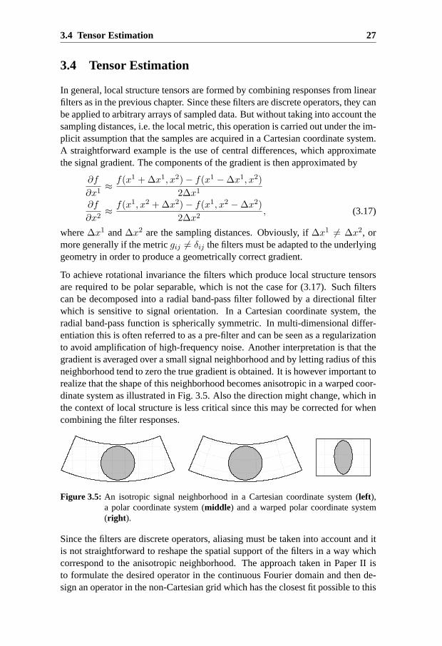
To achieve rotational invariance the filters which produce local structure tensorsare required to be polar separable, which is not the case for (3.17). Such filterscan be decomposed into a radial band-pass filter followed by a directional filterwhich is sensitive to signal orientation. In a Cartesian coordinate system, theradial band-pass function is spherically symmetric. In multi-dimensional differ-entiation this is often referred to as a pre-filter and can be seen as a regularizationto avoid amplification of high-frequency noise. Another interpretation is that thegradient is averaged over a small signal neighborhood and by letting radius of thisneighborhood tend to zero the true gradient is obtained. It is however important torealize that the shape of this neighborhood becomes anisotropic in a warped coor-dinate system as illustrated in Fig. 3.5. Also the direction might change, which inthe context of local structure is less critical since this may be corrected for whencombining the filter responses.
Figure 3.5: An isotropic signal neighborhood in a Cartesian coordinate system (left),a polar coordinate system (middle) and a warped polar coordinate system(right ).
Since the filters are discrete operators, aliasing must be taken into account and itis not straightforward to reshape the spatial support of the filters in a way whichcorrespond to the anisotropic neighborhood. The approach taken in Paper II isto formulate the desired operator in the continuous Fourier domain and then de-sign an operator in the non-Cartesian grid which has the closest fit possible to this

28 Chapter 3. Non-Cartesian Local Structure
desired frequency response. For practical reasons this approachwas limited fornon-Cartesian coordinate systems which locally are well described by an affinetransformation. This is because the the Shannon sampling theorem is still appli-cable for such transformations. There are, however, sampling theoremsthat allowmore general transformations as long as the signal band-limitedness is preserved(see Unser (2000)).
As a result of this procedure, the local structure tensor field can be estimatedin the warped coordinate system. In Fig. 3.6 the results for a patch estimatedfrom an ultrasound image are shown (Paper I). By studying the color code whichrepresents signal orientation, it is fairly easy to see that this approach produce aplausible tensor field. Note also that the geometric distortion is far from beingnegligible. In the lower parts of the image, the pixels in the geometrically correctimage are stretched approximately4 times compared to the original grid.
Figure 3.6: Top: An ultrasound image acquired in a polar coordinate system, resampledto a correct geometry (left) and in its original sampling grid, i.e. a warpedcoordinate system (right ). Bottom: A local structure tensor field estimatedfrom the warped coordinate system, transformed and resampled to to a cor-rect geometry (left) and in its original sampling grid (right ). The color rep-resent the orientation of the major axis in the correct geometry.
3.5 Discussion 29
3.5 Discussion
Under the assumption that the underlying geometry is important, one must dis-tinguish between covariant and contravariant tenors in non-Cartesian coordinatesystems. For a geometrically correct description of local structure, the tensor fieldmust be transformed in accordance to theory. However, by utilizing a spatiallyvarying metric eigenvalue analysis can be performed in a warped image withouttransforming the tensor field.
The limitations brought on by only having access to sampled data makes it dif-ficult to estimate a tensor, which in a strict sense is consistent with the theorypresented. The presented work relies on that the transformation between the coor-dinate systems can be approximated by an affine transformation, at least locally.
Experiments were carried out both on real data, an ultrasound image acquiredin a polar coordinate system, and synthetic data. For the synthetic data, moreaccurate estimates of the dominant orientation could be obtained with less amountof processing. The presented work is also applicable to curved manifolds providedthat they are locally flat, i.e. they must have a relatively low curvature.

4Tensor-Driven Noise Reduction
and Enhancement
Noise reduction is probably one of the most well-studied problems in image analy-sis and methods which incorporate information from local structure analysis havebeen suggested by many authors. The work in (Paper III) concerns one suchmethod called anisotropic adaptive filtering, which is here reviewed. This chapteralso briefly reviews the main ideas of a few existing methodologies, which makeuse of local structure or in other ways are related to anisotropic adaptive filtering.
4.1 Introduction
For multidimensional signals, in particular images, there exists a large amount ofmethods for denoising, edge-preserving smoothing, enhancement and restoration.The different terms are nuances of essentially the same problem and indicate ei-ther what type of method is used or what purpose the method serves. With smallmodifications the vast majority of methods fit under several of the above men-tioned categories.
Noise reduction, denoising and noise removal are more or less equivalent termsfor methods with the ideal goal of recovering a true underlying signal from an ob-served signal which is corrupted with random noise. Smoothing is a sub-categoryof denoising algorithms and generally refers to local filtering using an isotropiclow-pass filter. Typically, it is carried out by convolution with a Gaussian FIR fil-ter with the purpose of regularizing a signal. Smoothing in this sense will suppresshigh-frequency noise, but also high-frequency signal content. Since the signal-to-noise ratio of natural images is much lower for high frequencies, smoothing willreduce a large amount of noise and at the same time preserve most of the signalenergy. The human eye is, however, very sensitive to high frequency structuresand therefore it is, in image analysis, important to preserve high-frequency de-tails such as edges, lines and corners. Edge-preserving smoothing is a commonterm for filters which suppress high-frequency noise by smoothing, but avoid sup-pression of edges. Typically the smoothing process is stopped in regions where
32 Chapter 4. Tensor-Driven Noise Reduction and Enhancement
edges are present. An alternative is to allow high-frequency content locally, wherehigh-frequency signal content is detected.
In image restoration, knowledge about the degradation is utilized to recover thetrue underlying signal. In contrast to denoising, restoration may also address cor-rection of global degradation phenomena arisen during the imaging process suchas lens distortion and blurring. Also, removal of artifacts can be addressed. Typi-cally, these methods rely on estimated or known statistics. Image restoration canbe significantly more complex in comparison to noise reduction, since it may in-volve inverse problems. Image enhancement differs from image restoration anddenoising in the sense that it does not target the true underlying signal. In additionto noise reduction, the visibility of small structures can for instance be improvedby locally or globally changing the image histogram. The purpose is to make theimage as pleasing or as informative to the eye as possible. Evaluating enhance-ment is therefore very difficult, since the image quality is to a large extent a sub-jective measure. Algorithms for enhancement are usually more heuristic in theirnature and user interaction is very important. Enhancement is also commonlyused as a pre-processing step, where the goal is to make the image as suitable aspossible for a specific application.
The end user in medical image science is often a medical specialist, who typicallyencounters image enhancement. With a few parameters, provided by a graphicaluser interface, the goal is to enhance image structures of important clinical value.In medical imaging, denoising also plays a central part, since most imaging de-vices deliver processed data rather than raw data. For instance, a higher imagequality in computed tomography can in general be accomplished only if the radi-ation dose is increased, with undesirable side effects to the patient. In magneticresonance imaging, a similar trade-off exists between acquisition time and im-age quality. The goal of denoising is then to decrease the radiation dose or theacquisition time while maintaining the image quality.
In this chapter, the focus is mainly on adaptive anisotropic filtering which is a lowcomplexity methodology for image enhancement having a good post-processingsteerability which enables fast user interaction. Even though it is not primar-ily designed for noise reduction, it provides, in2D, a low complexity alternativewhich is competitive to the state-of-the-art. In3D the method is burdened bya substantially higher computational complexity, a problem which is addressedin (Paper III). The use of local structure analysis, estimated from a set of lin-ear filters, makes the algorithm an ideal example for illustrating the use of filternetworks presented in chapter 7. Before introducing this methodology, the mainideas of a few selected methodologies that relate to adaptive anisotropic filteringare presented.

4.2 Noise Reduction 33
4.2 Noise Reduction
Reducing noise in images is essentially a data fitting problem, which can be ap-proached with traditional regression algorithms. A simple synthetic1D exampleis shown in Fig. 4.1. A typical problem setup is a sampled ideal imagef which iscorrupted by additive uncorrelated noisen, which yields the linear signal model
y = f + n, (4.1)
wherey, f andn are vectors. The objective is to reduce or remove the noise inthe observed datay to get as close as possible tof . With knowledge about thesecond order statistics of signal and noise, the optimal linear operator in the leastsquares sense is obtained by solving the problem:
minf
E[‖f − f‖2
](4.2)
Assuming the covariance matricesCf = E[ffT
]andCn = E
[nnT
]= σ2I to
be known, the solution which minimizes this expected least squares distance is
f = Cf (Cf + Cn)−1y = (I + σ2C−1
f )−1y. (4.3)
This well-known solution is recognized as the Wiener filter solution and is underthe same assumptions also the minimizer to the equivalent problem
minf
= ‖f − y‖2 + σ2‖C−1f f‖2. (4.4)
In estimation theory this technique is known as Tikhonov regularization and instatistics as ridge regression. The fundamental problem with this technique is theunderlying assumption of wide-sense stationary noise and signal characteristics.Most interesting signals violate these assumptions, since characteristics changewith spatial position. Therefore, the global approach of classic Wiener filtering isconsidered insufficient for noise reduction of general images.
Figure 4.1: Noise reduction is essentially a data fitting problem.Left: Original syntheticsignal. Right: The result of a local adaptive Wiener filter applied to noisymeasurements (gray dots).
Most methods for noise reduction can be categorized as either transform-based oras PDE-based, which are the two predominant ways to overcome the drawback

34 Chapter 4. Tensor-Driven Noise Reduction and Enhancement
of the stationarity assumption. By imposing constraints on the smoothness of thesolution, PDE-based methods and adaptive filters typically operate directly in thesignal domain. A different approach is transform-based methods, where the im-posed constraints are formulated as boundedness or sparsity in a feature space.The feature space is usually computed by applying a linear transform to the sig-nal. Other methods which are not included in this overview and deserve to bementioned are mean shift filters (Comaniciu and Meer, 2002), bilateral filtering(Tomasi and Manduchi, 1998) and non-local means (Buades et al., 2005). Forthe interested reader there are some quite recent papers, which establish connec-tions between different kinds of denoising techniques including adaptive filter-ing, wavelet shrinkage, variational formulations and PDE-based methods (Sochenet al., 1998; Scherzer and Weickert, 2000; Barash, 2002).
4.2.1 Transform-Based Methods
One of the most well-known regression techniques is dimension reduction by prin-cipal component analysis, also known as truncated singular value decompositionor as the Karhunen-Loeve transform. Analogous to Wiener filtering, the signal iswell described by a sub-space, in this case spanned by a few principal componentswhich are characterized by large principal values. Noise typically projects on allprincipal components and components which contain mostly noise are thereforecharacterized by small principal values. In contrast to Wiener filtering, where thecomponents characterized as noise are attenuated, the principal components withnegligible or no correlation with the signal are in dimension reduction truncatedto zero. In other words, an estimate off is obtained by thresholding in the trans-form domain and then the signal is reconstructed as an element in the sub-spacespanned by the remaining principal components.
The same idea is employed in wavelet denoising, where the change of basis iscomputed using a wavelet transform. To better describe local features, waveletpackets are waveforms of finite spatial size with an average value of zero. Thewavelet transform is computed by recursively applying scaled and translatedversions of the so called mother wavelet. The locality of each wavelet packetand the use of multiple scales make the wavelet basis better suited to capturenon-stationary signal characteristics. A general formulation of a transform-basedmethod due to (Elad, 2006) is
minf
‖f − y‖2 + λΨ(Wf), (4.5)
where the signal representation off in the transform domain is denoted byWf
andW defines the transformation. The functionΨ(·) is usually a robust normwhich favors sparsity such asΨ(·) = ‖ · ‖1.
With a unitary wavelet transform, the solution to problem (4.5) is obtained byshrinkage (Donoho, 1995), i.e. thresholding in the transform domain followed
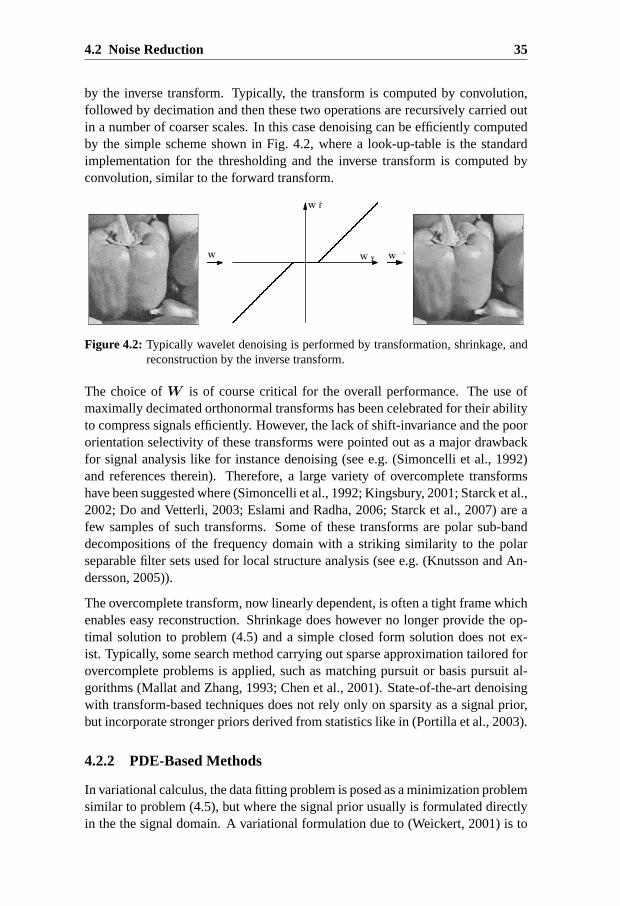
4.2 Noise Reduction 35
by the inverse transform. Typically, the transform is computed by convolution,followed by decimation and then these two operations are recursively carried outin a number of coarser scales. In this case denoising can be efficiently computedby the simple scheme shown in Fig. 4.2, where a look-up-table is the standardimplementation for the thresholding and the inverse transform is computed byconvolution, similar to the forward transform.
W y
W f
W W−1
Figure 4.2: Typically wavelet denoising is performed by transformation, shrinkage, andreconstruction by the inverse transform.
The choice ofW is of course critical for the overall performance. The use ofmaximally decimated orthonormal transforms has been celebrated for their abilityto compress signals efficiently. However, the lack of shift-invariance and the poororientation selectivity of these transforms were pointed out as a major drawbackfor signal analysis like for instance denoising (see e.g. (Simoncelli et al., 1992)and references therein). Therefore, a large variety of overcomplete transformshave been suggested where (Simoncelli et al., 1992; Kingsbury, 2001; Starck et al.,2002; Do and Vetterli, 2003; Eslami and Radha, 2006; Starck et al., 2007) are afew samples of such transforms. Some of these transforms are polar sub-banddecompositions of the frequency domain with a striking similarity to the polarseparable filter sets used for local structure analysis (see e.g. (Knutsson and An-dersson, 2005)).
The overcomplete transform, now linearly dependent, is often a tight frame whichenables easy reconstruction. Shrinkage does however no longer provide the op-timal solution to problem (4.5) and a simple closed form solution does not ex-ist. Typically, some search method carrying out sparse approximation tailored forovercomplete problems is applied, such as matching pursuit or basis pursuit al-gorithms (Mallat and Zhang, 1993; Chen et al., 2001). State-of-the-art denoisingwith transform-based techniques does not rely only on sparsity as a signal prior,but incorporate stronger priors derived from statistics like in (Portilla et al., 2003).
4.2.2 PDE-Based Methods
In variational calculus, the data fitting problem is posed as a minimization problemsimilar to problem (4.5), but where the signal prior usually is formulated directlyin the the signal domain. A variational formulation due to (Weickert, 2001) is to
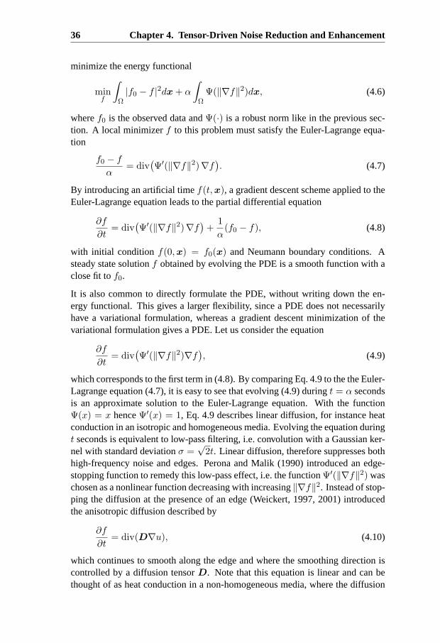
36 Chapter 4. Tensor-Driven Noise Reduction and Enhancement
minimize the energy functional
minf
∫
Ω|f0 − f |2dx + α
∫
ΩΨ(‖∇f‖2)dx, (4.6)
wheref0 is the observed data andΨ(·) is a robust norm like in the previous sec-tion. A local minimizerf to this problem must satisfy the Euler-Lagrange equa-tion
f0 − f
α= div
(Ψ′(‖∇f‖2)∇f
). (4.7)
By introducing an artificial timef(t,x), a gradient descent scheme applied to theEuler-Lagrange equation leads to the partial differential equation
∂f
∂t= div
(Ψ′(‖∇f‖2)∇f
)+
1
α(f0 − f), (4.8)
with initial condition f(0,x) = f0(x) and Neumann boundary conditions. Asteady state solutionf obtained by evolving the PDE is a smooth function with aclose fit tof0.
It is also common to directly formulate the PDE, without writing down the en-ergy functional. This gives a larger flexibility, since a PDE does not necessarilyhave a variational formulation, whereas a gradient descent minimization of thevariational formulation gives a PDE. Let us consider the equation
∂f
∂t= div
(Ψ′(‖∇f‖2)∇f
), (4.9)
which corresponds to the first term in (4.8). By comparing Eq. 4.9 to the the Euler-Lagrange equation (4.7), it is easy to see that evolving (4.9) duringt = α secondsis an approximate solution to the Euler-Lagrange equation. With the functionΨ(x) = x henceΨ′(x) = 1, Eq. 4.9 describes linear diffusion, for instance heatconduction in an isotropic and homogeneous media. Evolving the equation duringt seconds is equivalent to low-pass filtering, i.e. convolution with a Gaussian ker-nel with standard deviationσ =
√2t. Linear diffusion, therefore suppresses both
high-frequency noise and edges. Perona and Malik (1990) introduced an edge-stopping function to remedy this low-pass effect, i.e. the functionΨ′(‖∇f‖2) waschosen as a nonlinear function decreasing with increasing‖∇f‖2. Instead of stop-ping the diffusion at the presence of an edge (Weickert, 1997, 2001) introducedthe anisotropic diffusion described by
∂f
∂t= div(D∇u), (4.10)
which continues to smooth along the edge and where the smoothing direction iscontrolled by a diffusion tensorD. Note that this equation is linear and can bethought of as heat conduction in a non-homogeneous media, where the diffusion
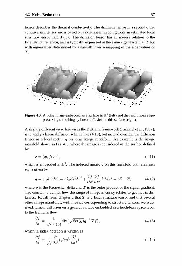
4.2 Noise Reduction 37
tensor describes the thermal conductivity. The diffusion tensor is a second ordercontravariant tensor and is based on a non-linear mapping from an estimated localstructure tensor fieldT (x). The diffusion tensor has an inverse relation to thelocal structure tensor, and is typically expressed in the same eigensystem asT butwith eigenvalues determined by a smooth inverse mapping of the eigenvalues ofT .
Figure 4.3: A noisy image embedded as a surface inR3 (left) and the result from edge-
preserving smoothing by linear diffusion on this surface (right ).
A slightly different view, known as the Beltrami framework (Kimmel et al., 1997),is to apply a linear diffusion scheme like (4.10), but instead consider the diffusiontensor as a local metricg on some image manifold. An example is the imagemanifold shown in Fig. 4.3, where the image is considered as the surface definedby
r =(x, f(x)
), (4.11)
which is embedded inR3. The induced metricg on this manifold with elementsgij is given by
g = gijdxidxj = εδijdx
idxj +∂f
∂xi∂f
∂xjdxidxj = εδ + T , (4.12)
whereδ is the Kronecker delta andT is the outer product of the signal gradient.The constantε defines how the range of image intensity relates to geometric dis-tances. Recall from chapter 2 thatT is a local structure tensor and that severalother image manifolds, with metrics corresponding to structure tensors, were de-rived. Linear diffusion on a general surface embedded in a Euclidean space leadsto the Beltrami flow
∂f
∂t=
1√
det(g)div
(√
det(g)g−1 ∇f), (4.13)
which in index notation is written as
∂f
∂t=
1√g
∂
∂xi(√ggij
∂f
∂xj). (4.14)
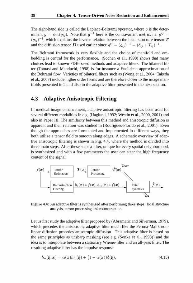
38 Chapter 4. Tensor-Driven Noise Reduction and Enhancement
The right-hand side is called the Laplace-Beltrami operator, whereg is the deter-minantg = det(gij). Note thatg−1 here is the contravariant metric, i.e.gij =(gij)
−1, which explains the inverse relation between the local structure tensorT
and the diffusion tensorD used earlier sincegij = (gij)−1 = (δij + Tij)
−1.
The Beltrami framework is very flexible and the choice of manifold and em-bedding is central for the performance. (Sochen et al., 1998) shows that manychoices lead to known PDE-based methods and adaptive filters. The bilateral fil-ter (Tomasi and Manduchi, 1998) is for instance a Euclidean approximation ofthe Beltrami flow. Varieties of bilateral filters such as (Wong et al., 2004; Takedaet al., 2007) include higher order forms and are therefore closer to the image man-ifolds presented in 2 and also to the adaptive filter presented in the next section.
4.3 Adaptive Anisotropic Filtering
In medical image enhancement, adaptive anisotropic filtering has been used forseveral different modalities in e.g. (Haglund, 1992; Westin et al., 2000, 2001) andalso in Paper III. The similarity between this method and anisotropic diffusion isapparent and their relation was studied in (Rodrigues-Florido et al., 2001). Eventhough the approaches are formulated and implemented in different ways, theyboth utilize a tensor field to smooth along edges. A schematic overview of adap-tive anisotropic filtering is shown in Fig. 4.4, where the method is divided intothree main steps. After these steps a filter, unique for every spatial neighborhood,is synthesized and with a few parameters the user can steer the high frequencycontent of the signal.
SynthesisFiltering
TensorProcessingEstimation
TensorUser
Reconstruction
f(x) T (x)
f(x)
T (x)
hi(x) ∗ f(x), hlp(x) ∗ f(x) Filter
Figure 4.4: An adaptive filter is synthesized after performing three steps: local structureanalysis, tensor processing and reconstruction.
Let us first study the adaptive filter proposed by (Abramatic and Silverman, 1979),which precedes the anisotropic adaptive filter much like the Perona-Malik non-linear diffusion precedes anisotropic diffusion. This adaptive filter is based onthe same principles as unsharp masking (see e.g. (Sonka et al., 1998)) and theidea is to interpolate between a stationary Wiener-filter and an all-pass filter. Theresulting adaptive filter has the impulse response
hα(ξ,x) = α(x)hlp(ξ) +(1 − α(x)
)δ(ξ), (4.15)

4.3 Adaptive Anisotropic Filtering 39
wherex are global image coordinates andξ are coordinates for the local neighbor-hood. Since the Wiener filter typically has low-pass characteristics it is denotedhlp. In contrast to unsharp masking, the so called visibility functionα ∈ [0, 1]varies with spatial position and determines locally, based on the image gradient,the amount of high-frequency content allowed to pass. This means that the filteris adaptive with respect to local bandwidth.
This filter was later extended in (Knutsson et al., 1981), where a filter adaptivealso with respect to orientation was presented. The basic principles employedlater became known as steerable filters (Freeman and Adelson, 1991). Furtherdevelopment has led to the adaptive anisotropic filter
hα(ξ,x) = hlp(ξ) +m∑
k=1
αk(x)hk(ξ) (4.16)
wherehk is a set of anisotropic filters andαk is controlled by a local structuretensor field (Knutsson et al., 1991). By applying the adaptive filter to the output ofa multi-scale image pyramid and interpolating between the different enhancementresults, this filter was also made adaptive with respect to scale (Haglund, 1992).For the remaining part of this section let us however restrict the presentation tothe single-scale version of this adaptive anisotropic filter.
4.3.1 Local Structure Analysis
A tensorT constitutes a local signal model designed to describe intrinsically1Dsignal neighborhoods. This local model features rotational invariance, i.e. signalneighborhoods are treated the same way regardless of orientation and with excel-lent angular selectivity.
A large tensor norm‖T (x)‖ indicates a well-defined local structure. With a filterset, where the number of filters is larger than the degrees of freedom of the ten-sor, it is possible to detect signal neighborhoods that do not fit the signal model.This is important in order to avoid introduction of artifacts. Such neighborhoodsare typically characterized by more or less isotropic tensors with a large normMoreover, the partly redundant information provided by this filter set, also allowsconstruction of a local model which is insensitive to the signal phase. This meansthat for instance high-frequency details such as edges and lines will be treated inthe same way.
A structure tensor of rank less than the signal dimensiond indicates a signal neigh-borhood of intrinsic dimensionality less thand. Similar to anisotropic diffusionthis enables smoothing in direction orthogonal to the signal orientation.
A local structure tensor field is constructed from a set of filter responses as de-scribed in the previous two chapters. This set of filters constitutes an isotropicpolar sub-band decomposition of the frequency domain and the anisotropic re-construction filters are typically obtained with a similar set of filters.

40 Chapter 4. Tensor-Driven Noise Reduction and Enhancement
4.3.2 Tensor Processing
There are many possibilities to process the estimated tensor field in order to en-hance or attenuate different image structures. Typical operations are element-wisemultiplications and tensor averaging. More sophisticated tools for tensor process-ing have appeared quite recently, which might be of interest for future develop-ment such asP -averages (Herberthson et al., 2007), bilateral filtering (Hamarnehand Hradsky, 2007), morphological operations (Burgeth et al., 2004). However,for the tools to be useful the computational complexity of such an operation mustnot be too large.
Recall from the transform-based methods how thresholding was used in orderto reduce the amount of high-frequency noise. Here, noise is characterized bytensors with small norm, whereas salient signal neighborhoods have large tensornorms. Soft thresholding of the tensor norm as in (Granlund and Knutsson, 1995),then produces a tensor field described by
T (x) =γ(‖T (x)‖)‖T (x)‖ T (x). (4.17)
where,γ is a low-parametric sigmoid-type function defined forx ∈ [0, 1] by
γ(x) =xβ
xα+β + σβ. (4.18)
As opposed to thresholding individual filter coefficients as in Sec. 4.2.1 only thetensor norm is here considered. This implies that the orientation is preserved andthe operation only controls the high-pass energy of the adaptive filter. A few sam-ples of the functionγ with different parameter settings are shown in Fig. 4.5. Hereσ plays a central role and defines the location of the threshold, which should cor-respond to the level of random noise. The slope of the transition or the ’softness’is defined byβ. The constantα typically ranges within[0, 0.5] and is used toaccentuate low-contrast structures just above the noise level threshold.
The orientation selectivity or the degree of anisotropy can in a similar way becontrolled globally by measuring and adjusting the eigenvalue ratiosλn
λn−1, where
λn−1 > λn andn > 1. In 3D a plane-like and a line-like neighborhood arecharacterized by the eigenvaluesλ1 ≫ λ2 ≈ λ3 andλ1 ≈ λ2 ≫ λ3 respectively.Such structures can then be attenuated or enhanced by
T (x) = T (x) +(µ( λn
λn−1)λn−1 − λn
)ene
Tn , (4.19)
whereen is the eigenvector corresponding toλn andµ is the smooth mapping
µ(x) =xβ(1 − α)β
xβ(1 − α)β + αβ(1 − x)β. (4.20)

4.3 Adaptive Anisotropic Filtering 41
‖T‖
γ(‖T‖)
σλn
λn−1
µ( λn
λn−1
)
α
Figure 4.5: Left: The functionγ(x) for a few different parameter settings.Right: Thefunctionµ(x) for a few different parameter settings.
This mapping is shown in Fig. 4.5 and the threshold here is defined byα, whichsatisfiesµ(α) = 1
2 . The constantβ is the slope ofγ for this point and hencedefines how soft the thresholding is.
Element-wise smoothing of the tensor componentsTij prevents rapid changes ofthe tensor field. This operation is carried out by the convolution
Tij(x) = g(x) ∗ Tij(x), (4.21)
whereg typically is a small isotropic low-pass kernel. Observe that this operationdoes not smooth the image content. If, for instance, two neighboring anisotropictensors differ in orientation, their average is a less anisotropic tensor. This impliesan adaptive filter with wider orientation selectivity, which for a salient structuremeans that a larger amount of of high-frequency content is allowed to pass.
4.3.3 Reconstruction and Filter Synthesis
The set of anisotropic filtershk used for reconstruction filters belong to the sameclass of polar separable filters as the ones used for local structure analysis. Filtersof odd order are in general not used for reconstruction. This is because they causean, in this case, undesirable phase-shift of the signal, whereas filters of even orderpreserve the signal phase. The radial function of the anisotropic filters has high-pass characteristics and for perfect reconstruction the sum of all reconstructionfilters must satisfy the equation
hlp(ξ) +
m∑
k=1
hk(ξ) = δ(ξ). (4.22)
For practical reasons it is convenient to use the same directional functions as thesecond order filters used for producing the tensor field.
42 Chapter 4. Tensor-Driven Noise Reduction and Enhancement
Instead of applying an inverse transform to reconstruct the signal, the tensor fieldis used to synthesize a filter which is locally adapted to the estimated signal model.This is accomplished by first computing the filter responsesfk(x) = f(x)∗hk(x)and also the response of the low-pass filter, i.e.flp = hlp(x)∗f(x). Then a linearcombinationα1, . . . , αm of the high-pass content is added to the smoothed imageflp by:
f(x) = flp(x) +m∑
k=1
αk(x)fk(x) (4.23)
The main advantage of this approach is that a change of the parameter settingsfor γ andµ requires a new linear combinationαk, but the computationally moreexpensive steps of this algorithm do not need to be recomputed. This allows theuser to steer the high-frequency content of a2D signal in real-time.
The scalar valuesαk are obtained by projecting the tensor field onto a set of dualtensorsMk, i.e. the adaptive filter in (4.23) can be expressed in terms of the localstructure tensor field:
f(x) = flp(x) +m∑
k=1
〈T ,Mk〉fk(x) (4.24)
The dual tensorsMk can be computed analytically or be estimated from a trainingset with ground truth as in (Andersson et al., 2001). The advantage of the latterapproach is that it is possible to compensate for filter distortion and take intoaccount prior knowledge about the distribution of signal and noise.
LetSi be the ideal local structure tensors for a training set of image patchesgi(x),wherei = 1, . . . , n. By computing all the filter responsesgki = hk(x) ∗ gi(x)for all n image patches, the dual tensors are obtained by solving the least squaresproblem
minM1,...,Mm
n∑
i=1
‖Si −m∑
k=1
gkiMk‖2. (4.25)
The analytical solution is obtained by solving the same problem, where the train-ing setSi is the orthonormal basis spanning the space of symmetric positive defi-nite tensors and the corresponding filter responses are computed with ideal filters.In the cases where there is no unique solution to problem (4.25), i.e.n < m, thesolutionM1, . . . ,Mm with minimum norm is preferred.
4.4 Discussion
Following a recent trend, to establish connections between different techniqueswith the goal to see what can be learnt from methods developed using disparate

4.4 Discussion 43
frameworks, a few methodologies for noise reduction were here reviewed. Theselected samples of methodologies have in common that they are related either tolocal structure analysis or the adaptive anisotropic filtering presented. The mainreasons for this particular choice are to identify other algorithms which may ben-efit from the results of this dissertation and to inspire to new ideas of how to makeuse of local structure.
In summary, the filter set used for local structure analysis is very close to someof the existing bases used for wavelet denoising. The soft thresholding used forthresholding wavelet coefficients and also the smooth mapping used in anisotropicdiffusion resembles the one used in adaptive filtering. In the context of variationaland diffusion frameworks anisotropic adaptive filtering can be interpreted as a sin-gle large time step. An important improvement of this adaptive filter is the use offilter networks (see chapter 7) producing3D filters for both local structure analysisand the reconstruction filtering, which significantly speeds up the computationallyintense part of this algorithm.

5FIR Filter Design
This chapter is an introduction to design of finite impulse response filters andprovides a background, necessary for the remaining chapters and also for PaperII, IV, V and VI. Contradictory demands on the desired frequency response andthe spatial locality make FIR filter design a delicate problem. Here, least squaresdesign criteria in multiple domains are used to obtain a localized filter, which isas close as possible to the frequency response for the expected signal and noisefrequency content.
5.1 Introduction
In chapter 2 a number of operators such as the image gradient, the Hilbert trans-form, the Riesz transform and the local structure tensor was presented. Thischapter provides a background for how such operators can be realized with fi-nite impulse response filters intended for sampled signals. For natural reasonsthese filters are digital. They are discrete in the spatial domain, but are treated ascontinuous in the image space, i.e. for each discrete spatial position a filter takeson a real value. By construction they can only form linear operators, which limittheir ability to realize non-linear operators. Still many non-linear operators, likefor instance the local structure tensor is computed from a non-linear combinationof linear filter responses. Also solutions to partial differential equations are oftenobtained by iteratively combining responses from linear filters. The process ofdesigning a filter is to form a realization of the filter which is as close as possibleto the desired operator. This can be formulated as an optimization problem, withthe goal to satisfy a set of requirements. This set of requirements define the met-ric for this search space, i.e. it defines what is meant by the term ’close’. Due tothe nature of this metric, it is common that the solution which is closest to the de-sired operator is a compromise between requirements that are partly contradictory.Common requirements for multidimensional FIR filters are:
46 Chapter 5. FIR Filter Design
Frequency characteristics: Since desired operators often are derived us-ing spatio-temporal statistics it is convenient to express the desired filter inthe Fourier domain as a frequency response, since it best describes shift-invariant characteristics. Even though the signals under consideration arediscrete, the Fourier transform of such signals are a continuous functions,which are periodic with a periodicity equal to the sampling frequency. Fre-quencies above the Nyquist frequency are aliased, which is why most filtersare restricted to specific frequency sub-bands.
Spatial characteristics: The spatial domain describes best local charac-teristics of a filter. Since there is a one-to-one correspondence betweenthe frequency response and the discrete impulse response defined by theFourier transform, it is sufficient to describe the filter entirely in one do-main. However, many filters do not have a closed form expression in thespatio-temporal domain. If such an expression exists it is rarely of finiteextension and may be difficult to realize efficiently.
Locality: For several reasons it is desirable keep the spatial support of thefilter small. A small filter implies a smaller computational load, due to fewernon-zero filter coefficients. More importantly, smaller filters maintain theresolution of the signal better. Furthermore, a filter typically represents alocal signal model with few degrees of freedom. A filter with small effectivesize is then more likely to fit the signal locally.
Computational complexity: The computation time for filtering are oftencritical in multidimensional signal processing, since it in general involvesa huge amount of data. There are two basic ways of implementing linearfiltering, either by convolution or by the use of the Fast Fourier Transform.The latter is sometimes referred to as fast convolution, which might be mis-leading since convolution is in general faster for small filters. The com-putational load of convolution-based filtering is defined by the number offilter coefficients. The aim of this and the sub-sequent two chapters is toreduce the number of filter coefficients required, and thereby reducing thecomputation time, without sacrificing any of the above requirements.
Symmetry requirements: Symmetry requirements are often implicitly de-fined by the desired frequency response and thus not necessary to take intoaccount. However, correctly imposed constraints on symmetries reduce thenumber of variables in the optimization problem and can improve the solu-tion since numerical errors can be avoided.
Traditionally, digital filters are divided into two categories, finite impulse responsefilters (FIR) and infinite impulse response filters (IIR). In1D an output sample ofa casual FIR filter is a weighted sum of the previous signal samples. In contrast tothe FIR filter an IIR filter makes use of feedback loops, i.e. the IIR filter reuses oneor several of the previous output samples recursively. Such filters are, however,
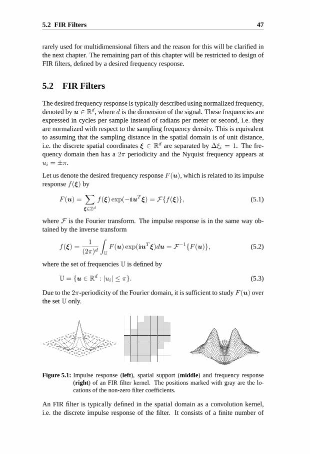
5.2 FIR Filters 47
rarely used for multidimensional filters and the reason for this will be clarified inthe next chapter. The remaining part of this chapter will be restricted to design ofFIR filters, defined by a desired frequency response.
5.2 FIR Filters
The desired frequency response is typically described using normalized frequency,denoted byu ∈ R
d, whered is the dimension of the signal. These frequencies areexpressed in cycles per sample instead of radians per meter or second, i.e. theyare normalized with respect to the sampling frequency density. This is equivalentto assuming that the sampling distance in the spatial domain is of unit distance,i.e. the discrete spatial coordinatesξ ∈ R
d are separated by∆ξi = 1. The fre-quency domain then has a2π periodicity and the Nyquist frequency appears atui = ±π.
Let us denote the desired frequency responseF (u), which is related to its impulseresponsef(ξ) by
F (u) =∑
ξ∈Zd
f(ξ) exp(−ııuT ξ) = Ff(ξ), (5.1)
whereF is the Fourier transform. The impulse response is in the same way ob-tained by the inverse transform
f(ξ) =1
(2π)d
∫
U
F (u) exp(ııuT ξ)du = F−1F (u), (5.2)
where the set of frequenciesU is defined by
U = u ∈ Rd : |ui| ≤ π. (5.3)
Due to the2π-periodicity of the Fourier domain, it is sufficient to studyF (u) overthe setU only.
Figure 5.1: Impulse response (left), spatial support (middle) and frequency response(right ) of an FIR filter kernel. The positions marked with gray are the lo-cations of the non-zero filter coefficients.
An FIR filter is typically defined in the spatial domain as a convolution kernel,i.e. the discrete impulse response of the filter. It consists of a finite number of
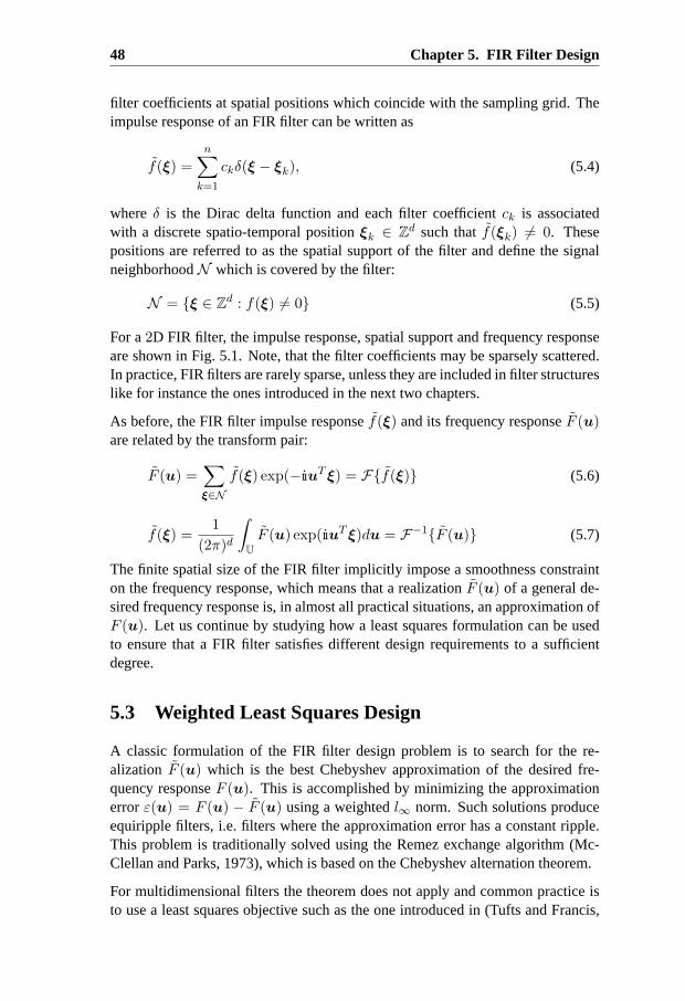
48 Chapter 5. FIR Filter Design
filter coefficients at spatial positions which coincide with the sampling grid. Theimpulse response of an FIR filter can be written as
f(ξ) =n∑
k=1
ckδ(ξ − ξk), (5.4)
whereδ is the Dirac delta function and each filter coefficientck is associatedwith a discrete spatio-temporal positionξk ∈ Z
d such thatf(ξk) 6= 0. Thesepositions are referred to as the spatial support of the filter and define the signalneighborhoodN which is covered by the filter:
N = ξ ∈ Zd : f(ξ) 6= 0 (5.5)
For a2D FIR filter, the impulse response, spatial support and frequency responseare shown in Fig. 5.1. Note, that the filter coefficients may be sparsely scattered.In practice, FIR filters are rarely sparse, unless they are included in filter structureslike for instance the ones introduced in the next two chapters.
As before, the FIR filter impulse responsef(ξ) and its frequency responseF (u)are related by the transform pair:
F (u) =∑
ξ∈N
f(ξ) exp(−ııuT ξ) = Ff(ξ) (5.6)
f(ξ) =1
(2π)d
∫
U
F (u) exp(ııuT ξ)du = F−1F (u) (5.7)
The finite spatial size of the FIR filter implicitly impose a smoothness constrainton the frequency response, which means that a realizationF (u) of a general de-sired frequency response is, in almost all practical situations, an approximation ofF (u). Let us continue by studying how a least squares formulation can be usedto ensure that a FIR filter satisfies different design requirements to a sufficientdegree.
5.3 Weighted Least Squares Design
A classic formulation of the FIR filter design problem is to search for the re-alization F (u) which is the best Chebyshev approximation of the desired fre-quency responseF (u). This is accomplished by minimizing the approximationerrorε(u) = F (u) − F (u) using a weightedl∞ norm. Such solutions produceequiripple filters, i.e. filters where the approximation error has a constant ripple.This problem is traditionally solved using the Remez exchange algorithm (Mc-Clellan and Parks, 1973), which is based on the Chebyshev alternation theorem.
For multidimensional filters the theorem does not apply and common practice isto use a least squares objective such as the one introduced in (Tufts and Francis,
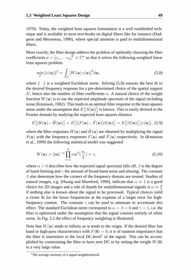
5.3 Weighted Least Squares Design 49
1970). Today, the weighted least squares formulation is a well established tech-nique and is available in most text-books on digital filters like for instance (Dud-geon and Mersereau, 1990), where special attention is paid to multidimensionalfilters.
More exactly, the filter design address the problem of optimally choosing the filtercoefficientsc = [c1, . . . cn]
T ∈ Cn so that it solves the following weighted linear
least squares problem
minc
‖ε(u)‖2 =
∫
U
∣∣W (u) ε(u)
∣∣2du, (5.8)
where‖ · ‖ is a weighted Euclidean norm. Solving (5.8) ensures the best fit tothe desired frequency response for a pre-determined choice of the spatial supportN , hence also the number of filter coefficientsn. A natural choice of the weightfunctionW (u) is to use the expected amplitude spectrum of the signal includingnoise (Knutsson, 1982). This leads to an optimal filter response in the least squaressense under the assumption thatE
[|S(u)|
]is known. This is easily derived in the
Fourier domain by studying the expected least squares distance
E[|H(u)−H(u)|
]= E
[|(F (u)− F (u)
)S(u)|
]= E
[|S(u)|
] ∣∣ε(u)
∣∣, (5.9)
where the filter responsesH(u) andH(u) are obtained by multiplying the signalS(u) with the frequency responsesF (u) and F (u) respectively. In (Knutssonet al., 1999) the following statistical model was suggested
W (u) = ‖u‖−αd∏
i=1
cosβ(ui2
) + γ, (5.10)
whereα > 0 describes how the expected signal spectrum falls off,β is the degreeof band-limiting andγ the amount of broad-band noise and aliasing. The constantβ also determine how the corners of the frequency domain are treated. Studies ofnatural images, e.g. (Huang and Mumford, 1999), indicate thatα ≈ 1 is a goodchoice for2D images and a rule of thumb for multidimensional signals isα ≈ d
2if nothing else is known about the signal to be processed. Typical choices yielda closer fit for the lower frequencies at the expense of a larger error for high-frequency content. The constantγ can be used to attenuate or accentuate thiseffect. The standard Euclidean norm correspond toα = β = 0 andγ = 1, i.e. thefilter is optimized under the assumption that the signal consists entirely of whitenoise. In Fig. 5.2 the effect of frequency weighting is illustrated.
Note thatW (u) tends to infinity asu tends to the origin. If the desired filter hasband or high-pass characteristics withF (0) = 0, it is of outmost importance thatthe filter is insensitive to the local DC-level1 of the signal. This can be accom-plished by constraining the filter to have zero DC or by setting the weightW (0)to a very large value.
1The average intensity of a signal neighbourhood.
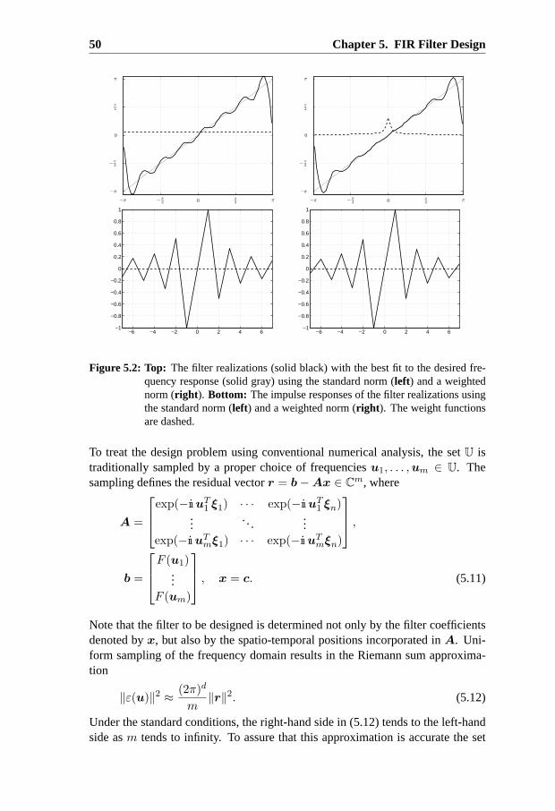
50 Chapter 5. FIR Filter Design
−π −π2 0
π2 π
−π
−π2
0
π2
π
−π −π2 0
π2 π
−π
−π2
0
π2
π
−6 −4 −2 0 2 4 6−1
−0.8
−0.6
−0.4
−0.2
0
0.2
0.4
0.6
0.8
1
−6 −4 −2 0 2 4 6−1
−0.8
−0.6
−0.4
−0.2
0
0.2
0.4
0.6
0.8
1
Figure 5.2: Top: The filter realizations (solid black) with the best fit to the desired fre-quency response (solid gray) using the standard norm (left) and a weightednorm (right ). Bottom: The impulse responses of the filter realizations usingthe standard norm (left) and a weighted norm (right ). The weight functionsare dashed.
To treat the design problem using conventional numerical analysis, the setU istraditionally sampled by a proper choice of frequenciesu1, . . . ,um ∈ U. Thesampling defines the residual vectorr = b − Ax ∈ C
m, where
A =
exp(−ııuT1 ξ1) · · · exp(−ııuT1 ξn)...
. . ....
exp(−ııuTmξ1) · · · exp(−ııuTmξn)
,
b =
F (u1)...
F (um)
, x = c. (5.11)
Note that the filter to be designed is determined not only by the filter coefficientsdenoted byx, but also by the spatio-temporal positions incorporated inA. Uni-form sampling of the frequency domain results in the Riemann sum approxima-tion
‖ε(u)‖2 ≈ (2π)d
m‖r‖2. (5.12)
Under the standard conditions, the right-hand side in (5.12) tends to the left-handside asm tends to infinity. To assure that this approximation is accurate the set
5.3 Weighted Least Squares Design 51
U must be sampled densely enough. The number of samples needed depends onhow smoothF (u) andF (u) are. Practical experience has shown that a good ruleof thumb is to at least havem > 2dn, i.e. the Fourier domain is sampled withtwice the number of samples per dimensionality compared to the spatial domain(Knutsson et al., 1999).
0
0.1
0.2
0.3
0.4
0.5
0.6
0.7
0.8
0.9
1
−π −π2 0
π2 π 1 2 3 4 5 6 7 8
0
0.02
0.04
0.06
0.08
0.1
0.12
Figure 5.3: Left: Riemann sum approximation of a lognormal band-pass filter withmsamples.Right: The estimated approximation error (black) compared to amore accurate estimate (gray) as a function ofm/n.
The relation (5.12) reduces (5.8), and hence the FIR filter design, to the linearleast squares problem
minx
‖b − Ax‖2. (5.13)
Here‖·‖ denotes a weighted Euclidean vector norm inRm, defined by the samples
W (ui) wherei = 1, . . . ,m. In Fig. 5.3 the approximation error‖b − Ax‖ forthex with the closest fit to a lognormal band-pass filter is shown as a function ofm/n with varyingm. Since this is an estimate of‖ε(u)‖, the approximation errorcan, for eachm, be estimated more accurately by computing‖b − A0x‖ for thesamex but whereA0 correspond to a constant number of samples, in this casem = 8n.
Now, recall that locality was listed in the set of requirements on an FIR filter inthe introduction of this chapter. With the least squares approach above, the spatialsupport and consequently also the filter size was pre-determined by the designer.But for a given spatial support, a filter can be made more localized by addinga regularization term (Knutsson et al., 1999). This approach can be posed as ageneralized Tikhonov regularization
minx
(1 − λ)‖b − Ax‖2W + λ‖x‖2
w, (5.14)
where‖ · ‖W is the vector norm introduced in (5.13) and the norm‖ · ‖w is aweighted Euclidean vector norm inRn defined by a functionw(ξi) in the spa-tial domain fori = 1, . . . , n. With a regularization term, which favors filters ofsmall effective size, the designer’s choice of the pre-determined spatial support
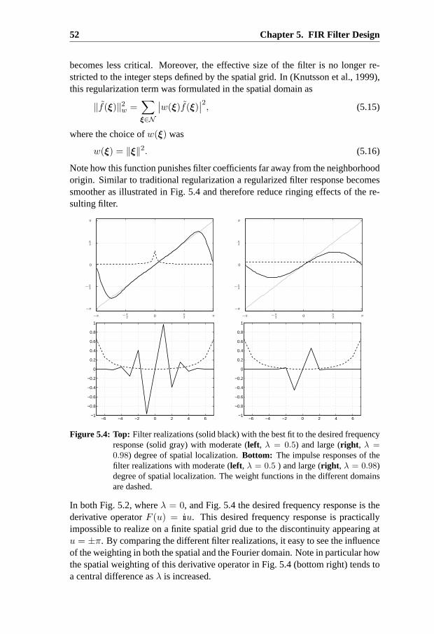
52 Chapter 5. FIR Filter Design
becomes less critical. Moreover, the effective size of the filter is no longer re-stricted to the integer steps defined by the spatial grid. In (Knutsson et al., 1999),this regularization term was formulated in the spatial domain as
‖f(ξ)‖2w =
∑
ξ∈N
∣∣w(ξ)f(ξ)
∣∣2, (5.15)
where the choice ofw(ξ) was
w(ξ) = ‖ξ‖2. (5.16)
Note how this function punishes filter coefficients far away from the neighborhoodorigin. Similar to traditional regularization a regularized filter response becomessmoother as illustrated in Fig. 5.4 and therefore reduce ringing effects of the re-sulting filter.
−π −π2 0
π2 π
−π
−π2
0
π2
π
−π −π2 0
π2 π
−π
−π2
0
π2
π
−6 −4 −2 0 2 4 6−1
−0.8
−0.6
−0.4
−0.2
0
0.2
0.4
0.6
0.8
1
−6 −4 −2 0 2 4 6−1
−0.8
−0.6
−0.4
−0.2
0
0.2
0.4
0.6
0.8
1
Figure 5.4: Top: Filter realizations (solid black) with the best fit to the desired frequencyresponse (solid gray) with moderate (left, λ = 0.5) and large (right , λ =0.98) degree of spatial localization.Bottom: The impulse responses of thefilter realizations with moderate (left, λ = 0.5 ) and large (right , λ = 0.98)degree of spatial localization. The weight functions in the different domainsare dashed.
In both Fig. 5.2, whereλ = 0, and Fig. 5.4 the desired frequency response is thederivative operatorF (u) = ııu. This desired frequency response is practicallyimpossible to realize on a finite spatial grid due to the discontinuity appearing atu = ±π. By comparing the different filter realizations, it easy to see the influenceof the weighting in both the spatial and the Fourier domain. Note in particular howthe spatial weighting of this derivative operator in Fig. 5.4 (bottom right) tends toa central difference asλ is increased.
5.4 Implementation 53
5.4 Implementation
Before moving on to more complex filter design problems, let us make a few re-marks concerning the least squares problem (5.14). This problem has an analyticalunique solution under the assumptions thatm ≥ n andA is of full rank. In termsof b andA the unique solutionxo is given by
xo = (A∗W 2A + w2)−1A∗W 2b, (5.17)
whereW andw are the diagonal matrices associated with the vector norms‖ ·‖W and‖ · ‖w. Numerically, there are a several ways to computexo which areboth numerically more stable and more efficient than explicitly computing (5.17).However, instead of focusing on numerical techniques let us study the properties,associated with filter design, which can be exploited to solve the least squaresproblem more efficiently.
Explicit computation ofxo can be expensive, especially for filters with signal di-mensionalitiesd > 2 where the matrixA typically is very large. Sincem > n, di-rect computation ofA∗W 2A of sizen×n is more appealing. This approach may,however, impair the relative accuracy of the solution. The elements of(A∗W 2A)are given by
(A∗W 2A)ij =∑
uk∈U
W 2(uk) exp(ııuTk (ξi − ξj)
). (5.18)
For dense1D filters this is a band matrix sinceξi − ξj is constant along the di-agonals. For the multidimensional case this property generalizes to a block bandmatrix and can be calculated using the inverse discrete Fourier transform. The useof sparse filters ruin this property, but since the number of admissible values isstill limited and defined by the unique spatial distancesξi − ξj the elements of(A∗W 2A) can still be pre-computed efficiently.
The special matrix structure of the Fourier operatorA can be exploited in moreways. Another option is to utilize that the Fourier operator is Cartesian separable.If also the weight functionsW andw are made Cartesian separable this propertyenables fast computation of the singular value decomposition, which can be usedto efficiently solve regularized least squares problems, see e.g. (Hansen et al.,2006). Note however that this is in direct conflict with the expected spectrum ofnatural images.
For the subsequent two chapters the most interesting alternative is to reduce thesize ofA and in particular the number of design variables. One option to de-crease the number of samplesm and consequently also the size ofA is to usenon-uniform sampling of the setU. The only modification of the least squaresformulation (5.14) necessary, is a redefinition of the vector norm‖ · ‖ such thatW (ui) = W (ui)vi wherevi is a volume associated withui.

54 Chapter 5. FIR Filter Design
The most efficient way reduce the size ofA is to exploit all known symmetryproperties of the desired frequency response and its impulse response. By enforc-ing constraints on symmetry bothm andn can be significantly decreased with apotentially dramatic reduction of the problem size. Let us consider the case whenthe filter, defined byA andx, is constrained to be rotationally symmetric in thespatial domain. The number of design variables inx can then reduced by
x = Cx, (5.19)
whereC ∈ Rn×n defines the coefficients that now are linearly dependent. For
a rotationally symmetric desired frequency response and with isotropic weightfunctions the best fit to the desired function is still in the set of feasible pointsx. Since the solution now is rotationally symmetric also the approximation errorε(ui) must be rotationally symmetric. Therefore it is sufficient to sample only thefrequencies such thatε(ui) is unique. All non-unique samples are removed byforming b ∈ C
m andA ∈ Cm×n. An accurate Riemann sum approximation to
‖ε(u)‖ is ensured by modifying the weight function such thatW (ui) = W (ui)+vi, wherevi now is the sum of weightsW (uj) for all non-unique samplesujassociated withui. For a typical FIR filter withn = 11d filter coefficients thesetU is sampled usingm = 35d samples. By enforcing rotational symmetry a4D filter can be designed with a modified Fourier operator of sizem = 1532timesn = 74 reduced by a factor1.9e5, i.e. an operator which is smaller than thestandard operator for the corresponding2D filter.
Most filters have symmetry properties, which can be exploited in a similar way.For instance the anisotropic filters used for local structure analysis are symmet-ric or anti-symmetric functions characterized byF (u) = F (−u) or F (u) =−F (−u). In addition to this property they are also rotationally symmetric aroundtheir main direction.
5.5 Experiments
Let us study two examples where the least squares framework can be slightlymodified to produce filters with additional requirements. Filters which are maxi-mally localized are sometimes of interest. An example is computation of spatialderivatives when evolving parabolic PDE:s, where a small step typically is desiredto ensure stability. By letting the regularization term dominate over the approxi-mation error in the frequency domain it is possible to design operators which haveminimal effective spatial size. The spatially most concentrated filter which ap-proximates a spatial derivative is recognized as the first order central difference,which was illustrated in Fig. 5.4. A more interesting example is the1D quadraturefilter with desired frequency response
F (u) =1
2
(
1 + sign(u))
, (5.20)
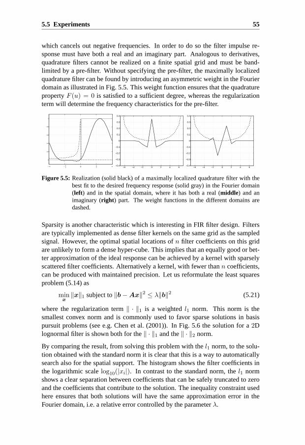
5.5 Experiments 55
which cancels out negative frequencies. In order to do so the filter impulse re-sponse must have both a real and an imaginary part. Analogous to derivatives,quadrature filters cannot be realized on a finite spatial grid and must be band-limited by a pre-filter. Without specifying the pre-filter, the maximally localizedquadrature filter can be found by introducing an asymmetric weight in the Fourierdomain as illustrated in Fig. 5.5. This weight function ensures that the quadraturepropertyF (u) = 0 is satisfied to a sufficient degree, whereas the regularizationterm will determine the frequency characteristics for the pre-filter.
0
0.2
0.4
0.6
0.8
1
−π −π2 0
π2 π −6 −4 −2 0 2 4 6
−0.4
−0.3
−0.2
−0.1
0
0.1
0.2
0.3
0.4
−6 −4 −2 0 2 4 6−0.4
−0.3
−0.2
−0.1
0
0.1
0.2
0.3
0.4
Figure 5.5: Realization (solid black) of a maximally localized quadrature filter with thebest fit to the desired frequency response (solid gray) in the Fourier domain(left) and in the spatial domain, where it has both a real (middle) and animaginary (right ) part. The weight functions in the different domains aredashed.
Sparsity is another characteristic which is interesting in FIR filter design. Filtersare typically implemented as dense filter kernels on the same grid as the sampledsignal. However, the optimal spatial locations ofn filter coefficients on this gridare unlikely to form a dense hyper-cube. This implies that an equally good or bet-ter approximation of the ideal response can be achieved by a kernel with sparselyscattered filter coefficients. Alternatively a kernel, with fewer thann coefficients,can be produced with maintained precision. Let us reformulate the least squaresproblem (5.14) as
minx
‖x‖1 subject to‖b − Ax‖2 ≤ λ‖b‖2 (5.21)
where the regularization term‖ · ‖1 is a weightedl1 norm. This norm is thesmallest convex norm and is commonly used to favor sparse solutions in basispursuit problems (see e.g. Chen et al. (2001)). In Fig. 5.6 the solution for a2Dlognormal filter is shown both for the‖ · ‖1 and the‖ · ‖2 norm.
By comparing the result, from solving this problem with thel1 norm, to the solu-tion obtained with the standard norm it is clear that this is a way to automaticallysearch also for the spatial support. The histogram shows the filter coefficients inthe logarithmic scalelog10(|xi|). In contrast to the standard norm, thel1 normshows a clear separation between coefficients that can be safely truncated to zeroand the coefficients that contribute to the solution. The inequality constraint usedhere ensures that both solutions will have the same approximation error in theFourier domain, i.e. a relative error controlled by the parameterλ.

56 Chapter 5. FIR Filter Design
−7 −6 −5 −4 −3 −2 −1 00
5
10
15
20
25
30
−12 −10 −8 −6 −4 −2 00
5
10
15
20
25
30
Figure 5.6: Frequency response (left), impulse response (middle) and histogram of thefilter coefficients in logarithmic scale (right ) for the lognormal band-passfilter using standard norm (top) and norm favoring sparsity (bottom).
5.6 Discussion
A least squares framework for design of finite impulse response filters was pre-sented in this chapter, where special attention was paid to the use of frequencyweighting and regularization which favors localized filters. The former ensuresthe best fit to the most common frequencies and the latter preserves the resolutionof the filtered signal as much as possible.
A common misbelief is that filter design address only filters which are imple-mented with convolution. The exact same operation can, however, be carried outby multiplication in the Fourier domain. In fact, one may argue that filter de-sign is even more important in the latter case. This is because multiplication withthe desired frequency response in the Fourier domain implicitly implies a filter ofthe same size as the signal itself, if the spatial size of the filter is not taken intoaccount. Such filters are not localized and may suffer badly from border effects.
The computational load of the filter was not part of the objective function in thisleast squares framework. The next two chapter concern filter realizations whichreduce this load. Even though sparse filters are very interesting for this purpose,the least squares formulation is still the most appealing one mainly because it leadsto a convex problem which can be solved by non-iterative methods. Moreover, it iseasy to incorporate additional filter requirements provided that they can expressedas linear constraints or objectives.

6Sub-Filter Sequences
Sub-filter sequences is a technique for efficient realization of linear filters. Thebasic idea is to carry out a sequence of convolutions with sparse sub-filters, whichfor multidimensional filters decreases the number of computations required for fil-tering. Design of sub-filter sequences is non-trivial, since the generalization of theleast squares formulation in the previous chapter yields a multi-linear least squaresproblem, which is highly ill-conditioned and has a large number of local minima.The approach presented in (Paper IV) for dealing with this multi-extremal natureis here reviewed with some additional experiments and details on the implemen-tation.
6.1 Introduction
The main advantage of finite impulse response filters treated in the previous chap-ter is the simple non-iterative design. The main disadvantage is the computationalload, in particular for multidimensional signals where the number of floating pointoperations required for filtering grows exponentially with the spatial dimension ofthe signal. It is well known that infinite impulse response filters (IIR) are far moreefficient in terms of computational load. Design of IIR filters is however morecomplex and typically involves additional requirements, such as causality and sta-bility, which must be satisfied to a sufficient degree.
Stability: A stable filter is a filter which for every bounded input yields abounded output. This is known as the BIBO requirement and is inherentlysatisfied for FIR filters since it does not make use of feedback loops.
Causality: A filter is causal if every output sample is dependent only onthe current and the past input samples. This definition presumes the filter tooperate in a temporal domain.
For multidimensional filters, causality is not a natural requirement. It implies aparticular ordering of the samples or a preferred filtering direction, similar to the
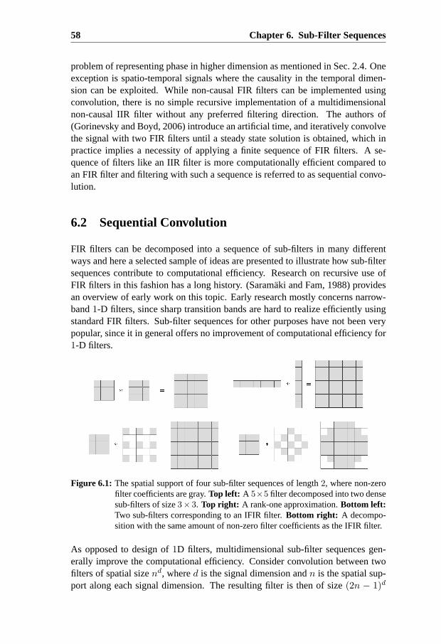
58 Chapter 6. Sub-Filter Sequences
problem of representing phase in higher dimension as mentioned in Sec. 2.4. Oneexception is spatio-temporal signals where the causality in the temporal dimen-sion can be exploited. While non-causal FIR filters can be implemented usingconvolution, there is no simple recursive implementation of a multidimensionalnon-causal IIR filter without any preferred filtering direction. The authors of(Gorinevsky and Boyd, 2006) introduce an artificial time, and iteratively convolvethe signal with two FIR filters until a steady state solution is obtained, which inpractice implies a necessity of applying a finite sequence of FIR filters. A se-quence of filters like an IIR filter is more computationally efficient compared toan FIR filter and filtering with such a sequence is referred to as sequential convo-lution.
6.2 Sequential Convolution
FIR filters can be decomposed into a sequence of sub-filters in many differentways and here a selected sample of ideas are presented to illustrate how sub-filtersequences contribute to computational efficiency. Research on recursive use ofFIR filters in this fashion has a long history. (Saramaki and Fam, 1988) providesan overview of early work on this topic. Early research mostly concerns narrow-band1-D filters, since sharp transition bands are hard to realize efficiently usingstandard FIR filters. Sub-filter sequences for other purposes have not been verypopular, since it in general offers no improvement of computational efficiency for1-D filters.
Figure 6.1: The spatial support of four sub-filter sequences of length2, where non-zerofilter coefficients are gray.Top left: A 5×5 filter decomposed into two densesub-filters of size3× 3. Top right: A rank-one approximation.Bottom left:Two sub-filters corresponding to an IFIR filter.Bottom right: A decompo-sition with the same amount of non-zero filter coefficients as the IFIR filter.
As opposed to design of1D filters, multidimensional sub-filter sequences gen-erally improve the computational efficiency. Consider convolution between twofilters of spatial sizend, whered is the signal dimension andn is the spatial sup-port along each signal dimension. The resulting filter is then of size(2n − 1)d
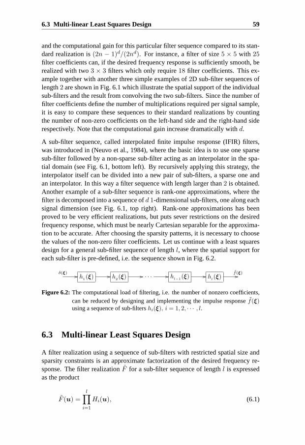
6.3 Multi-linear Least Squares Design 59
and the computational gain for this particular filter sequence compared to its stan-dard realization is(2n − 1)d/(2nd). For instance, a filter of size5 × 5 with 25filter coefficients can, if the desired frequency response is sufficiently smooth, berealized with two3 × 3 filters which only require18 filter coefficients. This ex-ample together with another three simple examples of2D sub-filter sequences oflength2 are shown in Fig. 6.1 which illustrate the spatial support of the individualsub-filters and the result from convolving the two sub-filters. Since the number offilter coefficients define the number of multiplications required per signal sample,it is easy to compare these sequences to their standard realizations by countingthe number of non-zero coefficients on the left-hand side and the right-hand siderespectively. Note that the computational gain increase dramatically withd.
A sub-filter sequence, called interpolated finite impulse response (IFIR) filters,was introduced in (Neuvo et al., 1984), where the basic idea is to use one sparsesub-filter followed by a non-sparse sub-filter acting as an interpolator in the spa-tial domain (see Fig. 6.1, bottom left). By recursively applying this strategy, theinterpolator itself can be divided into a new pair of sub-filters, a sparse one andan interpolator. In this way a filter sequence with length larger than2 is obtained.Another example of a sub-filter sequence is rank-one approximations, where thefilter is decomposed into a sequence ofd 1-dimensional sub-filters, one along eachsignal dimension (see Fig. 6.1, top right). Rank-one approximations has beenproved to be very efficient realizations, but puts sever restrictions on the desiredfrequency response, which must be nearly Cartesian separable for the approxima-tion to be accurate. After choosing the sparsity patterns, it is necessary to choosethe values of the non-zero filter coefficients. Let us continue with a least squaresdesign for a general sub-filter sequence of lengthl, where the spatial support foreach sub-filter is pre-defined, i.e. the sequence shown in Fig. 6.2.
δ(ξ)// h
1(ξ) // h
2(ξ) // · · · // h
l−1(ξ) // h
l(ξ)
f(ξ)//
Figure 6.2: The computational load of filtering, i.e. the number of nonzero coefficients,can be reduced by designing and implementing the impulse responsef(ξ)using a sequence of sub-filtershi(ξ), i = 1, 2, · · · , l.
6.3 Multi-linear Least Squares Design
A filter realization using a sequence of sub-filters with restricted spatial size andsparsity constraints is an approximate factorization of the desired frequency re-sponse. The filter realizationF for a sub-filter sequence of lengthl is expressedas the product
F (u) =l∏
i=1
Hi(u), (6.1)
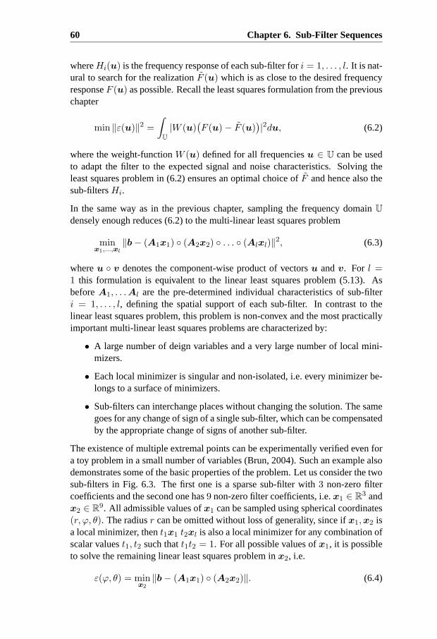
60 Chapter 6. Sub-Filter Sequences
whereHi(u) is the frequency response of each sub-filter fori = 1, . . . , l. It is nat-ural to search for the realizationF (u) which is as close to the desired frequencyresponseF (u) as possible. Recall the least squares formulation from the previouschapter
min ‖ε(u)‖2 =
∫
U
|W (u)(F (u) − F (u)
)|2du, (6.2)
where the weight-functionW (u) defined for all frequenciesu ∈ U can be usedto adapt the filter to the expected signal and noise characteristics. Solving theleast squares problem in (6.2) ensures an optimal choice ofF and hence also thesub-filtersHi.
In the same way as in the previous chapter, sampling the frequency domainU
densely enough reduces (6.2) to the multi-linear least squares problem
minx1,...,xl
‖b − (A1x1) (A2x2) . . . (Alxl)‖2, (6.3)
whereu v denotes the component-wise product of vectorsu andv. For l =1 this formulation is equivalent to the linear least squares problem (5.13). AsbeforeA1, . . .Al are the pre-determined individual characteristics of sub-filteri = 1, . . . , l, defining the spatial support of each sub-filter. In contrast to thelinear least squares problem, this problem is non-convex and the most practicallyimportant multi-linear least squares problems are characterized by:
• A large number of deign variables and a very large number of local mini-mizers.
• Each local minimizer is singular and non-isolated, i.e. every minimizer be-longs to a surface of minimizers.
• Sub-filters can interchange places without changing the solution. The samegoes for any change of sign of a single sub-filter, which can be compensatedby the appropriate change of signs of another sub-filter.
The existence of multiple extremal points can be experimentally verified even fora toy problem in a small number of variables (Brun, 2004). Such an example alsodemonstrates some of the basic properties of the problem. Let us consider the twosub-filters in Fig. 6.3. The first one is a sparse sub-filter with3 non-zero filtercoefficients and the second one has9 non-zero filter coefficients, i.e.x1 ∈ R
3 andx2 ∈ R
9. All admissible values ofx1 can be sampled using spherical coordinates(r, ϕ, θ). The radiusr can be omitted without loss of generality, since ifx1,x2 isa local minimizer, thent1x1 t2xl is also a local minimizer for any combination ofscalar valuest1, t2 such thatt1t2 = 1. For all possible values ofx1, it is possibleto solve the remaining linear least squares problem inx2, i.e.
ε(ϕ, θ) = minx2
‖b − (A1x1) (A2x2)‖. (6.4)
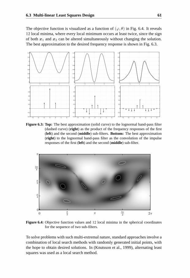
6.3 Multi-linear Least Squares Design 61
The objective function is visualized as a function of(ϕ, θ) in Fig. 6.4. It reveals12 local minima, where every local minimum occurs at least twice, since the signof bothx1 andx2 can be altered simultaneously without changing the solution.The best approximation to the desired frequency response is shown in Fig. 6.3.
0
0.2
0.4
0.6
0.8
1
1.2
1.4
−π − π2 0
π2 π
0
0.2
0.4
0.6
0.8
1
1.2
1.4
−π − π2 0
π2 π
0
0.2
0.4
0.6
0.8
1
1.2
1.4
−π − π2 0
π2 π
−6 −4 −2 0 2 4 6−0.4
−0.2
0
0.2
0.4
0.6
0.8
1
−6 −4 −2 0 2 4 6−0.4
−0.2
0
0.2
0.4
0.6
0.8
1
−6 −4 −2 0 2 4 6−0.4
−0.2
0
0.2
0.4
0.6
0.8
1
Figure 6.3: Top: The best approximation (solid curve) to the lognormal band-pass filter(dashed curve) (right ) as the product of the frequency responses of the first(left) and the second (middle) sub-filters.Bottom: The best approximation(right ) to the lognormal band-pass filter as the convolution of the impulseresponses of the first (left) and the second (middle) sub-filter.
0π2 π 3π
2 2π0
π4
π2
3π4
π
Figure 6.4: Objective function values and12 local minima in the spherical coordinatesfor the sequence of two sub-filters.
To solve problems with such multi-extremal nature, standard approaches involve acombination of local search methods with randomly generated initial points, withthe hope to obtain desired solutions. In (Knutsson et al., 1999), alternating leastsquares was used as a local search method.
62 Chapter 6. Sub-Filter Sequences
6.3.1 Alternating Least Squares
A practical way to solve a multi-linear least squares problem is to use a blockcoordinate descent method, i.e. compute a finite number of easy-to-solve sub-problems and iterate this procedure. In the context of multi-linear least squaresthis explicitly means that (6.3) is solved by sequentially solving the linear leastsquares sub-problems which are obtained by fixing all but one vectorxi, wherethe indexi is alternating. In this context the methodology is sometimes calledalternating least squares and the algorithm can be written in a few lines (see algo-rithm 1). Although each of the sub-problems is easy to solve the convergence isvery slow. In fact, this procedure does not even guarantee convergence to a localminimum.
Algorithm 1 Alternating Least Squares
Require: The desired frequency responseb ∈ Cm, initial sub-filter coefficients
xi ∈ Cni for i = 1, . . . , l and the Fourier operatorsAi ∈ C
m×ni , whichimplicitly defines the spatial support of each sub-filter.
Ensure: Sub-filter coefficientsxi which constitute a local minimum of the ob-jective function‖b − (A1x1) . . . (Alxl)‖2.repeat
for all sub-filtersxi, i = 1, . . . , l doFixate all but one vectorxi and compute:Ai =
( ∏
j 6=i diag(Ajxj))Ai
Solve the linear least squares sub-problem:xi = arg min ‖b − Aixi‖2
end foruntil convergence
Applying alternating least squares to the example shown in Fig. 6.4 from randominitial points is another way to reveal the number of local minimum and to obtain acourse estimate on the probability of finding the global minimum from an arbitraryinitial point. For this particular problem only8.6% of 1000 random initial pointsresults in the global minimum after100 iterations. Prior knowledge about thefilter to be realized is therefore important, but as them,n andl grows it becomesdifficult to guess a proper initial point. Therefore it is desirable to generate initialpoints which in this sense are more robust.
6.4 Generating Robust Initial Points
Randomly generated initial points often result in convergence to the same localsolutions. As soon as a local minimum is found, it is not reasonable to exert com-putational efforts to find the same local solution. Also, the convergence of localsearch methods is also very slow because the problem is highly ill-conditioned.
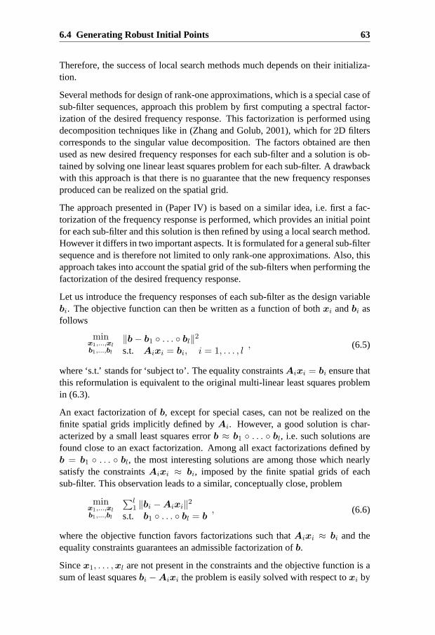
6.4 Generating Robust Initial Points 63
Therefore, the success of local search methods much depends on their initializa-tion.
Several methods for design of rank-one approximations, which is a special case ofsub-filter sequences, approach this problem by first computing a spectral factor-ization of the desired frequency response. This factorization is performed usingdecomposition techniques like in (Zhang and Golub, 2001), which for2D filterscorresponds to the singular value decomposition. The factors obtained are thenused as new desired frequency responses for each sub-filter and a solution is ob-tained by solving one linear least squares problem for each sub-filter. A drawbackwith this approach is that there is no guarantee that the new frequency responsesproduced can be realized on the spatial grid.
The approach presented in (Paper IV) is based on a similar idea, i.e. first a fac-torization of the frequency response is performed, which provides an initial pointfor each sub-filter and this solution is then refined by using a local search method.However it differs in two important aspects. It is formulated for a general sub-filtersequence and is therefore not limited to only rank-one approximations. Also, thisapproach takes into account the spatial grid of the sub-filters when performing thefactorization of the desired frequency response.
Let us introduce the frequency responses of each sub-filter as the design variablebi. The objective function can then be written as a function of bothxi andbi asfollows
minx1,...,xlb1,...,bl
‖b − b1 . . . bl‖2
s.t. Aixi = bi, i = 1, . . . , l, (6.5)
where ‘s.t.’ stands for ‘subject to’. The equality constraintsAixi = bi ensure thatthis reformulation is equivalent to the original multi-linear least squares problemin (6.3).
An exact factorization ofb, except for special cases, can not be realized on thefinite spatial grids implicitly defined byAi. However, a good solution is char-acterized by a small least squares errorb ≈ b1 . . . bl, i.e. such solutions arefound close to an exact factorization. Among all exact factorizations defined byb = b1 . . . bl, the most interesting solutions are among those which nearlysatisfy the constraintsAixi ≈ bi, imposed by the finite spatial grids of eachsub-filter. This observation leads to a similar, conceptually close, problem
minx1,...,xlb1,...,bl
∑l1 ‖bi − Aixi‖2
s.t. b1 . . . bl = b, (6.6)
where the objective function favors factorizations such thatAixi ≈ bi and theequality constraints guarantees an admissible factorization ofb.
Sincex1, . . . ,xl are not present in the constraints and the objective function is asum of least squaresbi − Aixi the problem is easily solved with respect toxi by
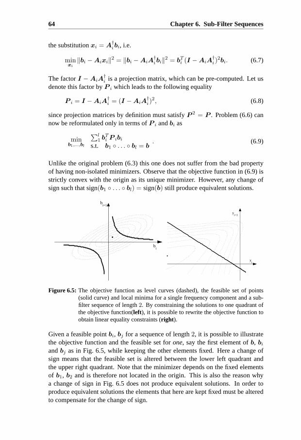
64 Chapter 6. Sub-Filter Sequences
the substitutionxi = A†ibi, i.e.
minxi
‖bi − Aixi‖2 = ‖bi − AiA†ibi‖2 = bTi (I − AiA
†i )
2bi. (6.7)
The factorI − AiA†i is a projection matrix, which can be pre-computed. Let us
denote this factor byP i which leads to the following equality
P i = I − AiA†i = (I − AiA
†i )
2, (6.8)
since projection matrices by definition must satisfyP 2 = P . Problem (6.6) cannow be reformulated only in terms ofP i andbi as
minb1,...,bl
∑l1 bTi P ibi
s.t. b1 . . . bl = b. (6.9)
Unlike the original problem (6.3) this one does not suffer from the bad propertyof having non-isolated minimizers. Observe that the objective function in (6.9) isstrictly convex with the origin as its unique minimizer. However, any change ofsign such that sign(b1 . . . bl) = sign(b) still produce equivalent solutions.
bi
bi+1
yi
yi+1
Figure 6.5: The objective function as level curves (dashed), the feasible set of points(solid curve) and local minima for a single frequency component and a sub-filter sequence of length2. By constraining the solutions to one quadrant ofthe objective function(left), it is possible to rewrite the objective function toobtain linear equality constraints (right ).
Given a feasible pointbi, bj for a sequence of length2, it is possible to illustratethe objective function and the feasible set forone, say the first element ofb, biandbj as in Fig. 6.5, while keeping the other elements fixed. Here a change ofsign means that the feasible set is altered between the lower left quadrant andthe upper right quadrant. Note that the minimizer depends on the fixed elementsof b1, b2 and is therefore not located in the origin. This is also the reason whya change of sign in Fig. 6.5 does not produce equivalent solutions. In order toproduce equivalent solutions the elements that here are kept fixed must be alteredto compensate for the change of sign.
6.4 Generating Robust Initial Points 65
Suppose that the prior knowledge aboutb allows us to guess in which quadrant thetrue minimizer is located. Assume, without loss of generality, that this quadrantis characterized bybi > 0 and thatb > 0. With this additional constraint it ispossible to rewrite (6.9) by the substitutionbi = exp(yi):
miny1,...,yl
∑l1 exp(yi)
TP i exp(yi)
s.t.∑l
1 yi = ln(b)(6.10)
whereexp(·), ln(·) are component-wise operations. It is a minimization problemwith very simple equality constraints as illustrated in Fig. 6.5.
To proceed with a local search method such as the alternating least squares it isnecessary to compute an initial pointx1, . . . ,xl to the original problem. With asolutiony1, . . . ,yl to problem (6.10), the initial point is obtained by the projec-tions
xi = A†ibi, (6.11)
wherebi is the back-substitutionbi = exp(yi).
If it is not possible to guess which quadrant to explore, one must treat the choiceof quadrant as a binary problem, where a problem like (6.10) must be solved for anumber of quadrants. Prior knowledge of the filter characteristics and its structurehelps to facilitate substantially the solution process by focusing on a relativelysmall number of quadrants. A few examples are given in (Paper IV), where it ispossible to make a qualified guess of which quadrant to explore. In that case itis important to find a way to reduce the number of quadrants to explore. Anotherimportant detail is the use of regularization that prevents undesirable scaling prob-lems, which occurs since there are trivial asymptotic solutions to problem (6.9).Cases where elements ofb or bi is exactly equal to zero is also treated in moredetail in (Paper IV).
6.4.1 Implementation
Conventional optimization algorithms for linearly constrained optimization prob-lems typically rely on computation of the gradient of the objective function andalso the Hessian (Nocedal and Wright, 1999). For large-scale problems it maynot be reasonable to compute the exact Hessian of size(ml) × (ml) explicitly,since it is prohibitively large. It is often sufficient to provide a procedure for com-puting the Hessian-vector product. Therefore it is desirable to make use of thematrix structure of the Hessian for computational efficiency. Denote the objectivefunctionψ(y1, . . . ,yl), where
ψ(y1, . . . ,yl) =1
2
l∑
1
exp(yi)TP i exp(yi). (6.12)
66 Chapter 6. Sub-Filter Sequences
The gradient∇ψ = [ ∂ψ∂y1
, . . . , ∂ψ∂yl
]T is then defined by the partial derivatives
∂ψ
∂yi= (P i exp(yi)) exp(yi), (6.13)
where each partial derivative is independent ofyj for j 6= i. This leads to theblock-diagonal Hessian matrix
H =
∂2ψ∂y1∂y1
0 · · · 0
0. .. . . .
......
. .. . . . 0
0 · · · 0∂2ψ
∂yl∂yl
. (6.14)
Denote the block-diagonal terms
H i =∂2ψ
∂yi∂yi= diag(
∂ψ
∂yi) + diag(exp(yi))P idiag(exp(yi)). (6.15)
The block-diagonal terms contain the projection matricesP i of sizem×m, whichcan be represented efficiently by performing a QR-factorization of eachAi. WithAi = QiRi, whereQi ∈ R
m×ni the projection matrix is defined by
P i = I − QiQTi . (6.16)
With this strategy it is sufficient to store eachQi, which are pre-computed insteadof the significantly larger projection matrices. The gradient can be expressed interms ofQi as
∂ψ
∂yi=
(bi − Qi(Q
Ti bi)
) bi, (6.17)
where the back-substitutionbi = exp(yi) is used to obtain a more compact ex-pression. The gradient can be computed efficiently and require only two matrix-vector multiplications.
In the same way, it is possible to rewrite the Hessian matrix in terms ofbi andQi,where the block-diagonal termsH i are then defined by
H i = diag(∂ψ
∂yi+ bi bi) − diag(bi)QiQ
Ti diag(bi). (6.18)
The first term is a diagonal matrix, which can be used as a pre-conditioner for theHessian matrix and to carry out Hessian multiplications very efficiently by
H iv = (∂ψ
∂yi+ bi bi) v − bi
(
Qi
(QTi (bi v)
))
, (6.19)
wherev ∈ Rm is an arbitrary vector. This operation requires only two matrix-
vector multiplications.
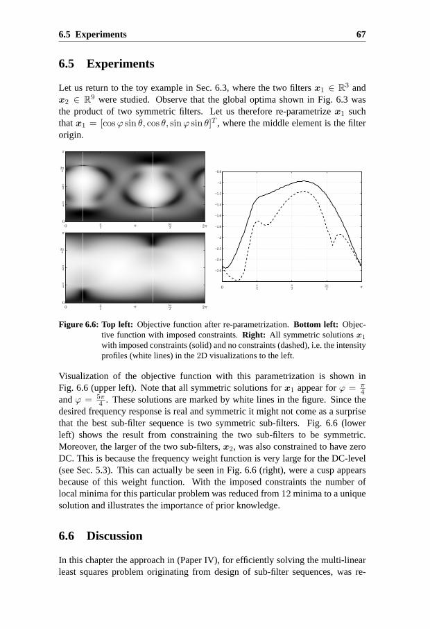
6.5 Experiments 67
6.5 Experiments
Let us return to the toy example in Sec. 6.3, where the two filtersx1 ∈ R3 and
x2 ∈ R9 were studied. Observe that the global optima shown in Fig. 6.3 was
the product of two symmetric filters. Let us therefore re-parametrizex1 suchthatx1 = [cosϕ sin θ, cos θ, sinϕ sin θ]T , where the middle element is the filterorigin.
0π2 π 3π
2 2π0
π4
π2
3π4
π
0π2 π 3π
2 2π0
π4
π2
3π4
π
−2.6
−2.4
−2.2
−2
−1.8
−1.6
−1.4
−1.2
−1
−0.8
0π4
π2
3π4
π
Figure 6.6: Top left: Objective function after re-parametrization.Bottom left: Objec-tive function with imposed constraints.Right: All symmetric solutionsx1
with imposed constraints (solid) and no constraints (dashed), i.e. the intensityprofiles (white lines) in the2D visualizations to the left.
Visualization of the objective function with this parametrization is shown inFig. 6.6 (upper left). Note that all symmetric solutions forx1 appear forϕ = π
4andϕ = 5π
4 . These solutions are marked by white lines in the figure. Since thedesired frequency response is real and symmetric it might not come as a surprisethat the best sub-filter sequence is two symmetric sub-filters. Fig. 6.6 (lowerleft) shows the result from constraining the two sub-filters to be symmetric.Moreover, the larger of the two sub-filters,x2, was also constrained to have zeroDC. This is because the frequency weight function is very large for the DC-level(see Sec. 5.3). This can actually be seen in Fig. 6.6 (right), were a cusp appearsbecause of this weight function. With the imposed constraints the number oflocal minima for this particular problem was reduced from12 minima to a uniquesolution and illustrates the importance of prior knowledge.
6.6 Discussion
In this chapter the approach in (Paper IV), for efficiently solving the multi-linearleast squares problem originating from design of sub-filter sequences, was re-
68 Chapter 6. Sub-Filter Sequences
viewed. This problem is highly ill-conditioned with a large number of local min-ima. The main focus here is to cope with the multi-extremal nature of this prob-lem, whereas the efficiency, for the moment, is of secondary importance. This isbecause it is known that a properly designed sub-filter sequence is more efficientcompared to conventional filtering but least squares design of such sequences,except for special cases, is less developed.
An efficient implementation of this approach is presented and experiments showhow prior knowledge can help to reduce the number of local minima. In (Pa-per IV) it is experimentally verified that the generated initial points provide goodrealizations for polar separable filters. The next chapter concerns design of fil-ter networks, a technique which is similar to the use of sub-filter sequences andfurther reduce the computational load of multidimensional filtering.

7Filter Networks
Filter networks is a technique for realization of multidimensional FIR filter sets. Itis characterized by a significantly lower computational load compared to standardconvolution. This chapter describes a multi-linear least squares formulation of thedesign problem associated with filter networks. The graph representation from(Paper VI) is used to derive an efficient local search method. A typical applicationof filter networks is feature extraction (Paper V), which is central for adaptivefiltering (Paper III).
7.1 Introduction
By decomposing a set of desired filters into a network of sparse sub-filters, it ispossible to reduce or eliminate redundant computations. This was observed in(Ahn et al., 1998), where an analogy between linear feed-forward networks andFIR filters was introduced. With a back-propagation algorithm and network prun-ing, multiple1D filters were realized with a decrease of the computational load. In(Andersson et al., 1999) filter networks was presented as a generalization of thetree-structured decompositions used for the vast majority of filter banks includ-ing wavelet transforms. The technique presented, allowed realization of2D filtersets with only a fraction of the computations required compared to conventionalfiltering techniques such as standard convolution. This was accomplished by ap-plying a local search method to ensure the closest fit between the output of a filternetwork and the desired frequency responses. Filter sets for3D was produced in(Paper V) using the same basic technique and will be reviewed in this chapter,which also includes more recent improvements.
Filter networks are in the following restricted to be single-rate1 systems and targetcomputationally efficient realizations of overcomplete linear transforms to be usedfor signal analysis. The possible computational gain is of course highly dependenton the transformation in mind, i.e. far from all linear transformations motivate the
1Single rate systems do not sub-sample the data to be processed.
70 Chapter 7. Filter Networks
use of filter networks. Filter networks typically target ’true’ multi-dimensionalfilter sets, e.g. filter sets where the desired filters are not Cartesian separable andhave at least2 spatial dimensions. For such filter sets, there are three fundamentalproperties of filter networks, which make them computationally efficient:
Low Redundancy: The network structure allows a single sub-filter to con-tribute to several output nodes. The basic idea is to exploit possible simi-larities between the filters in the set of desired frequency responses and toreuse intermediate results stored in the nodes of the network as much aspossible in order to reduce redundant computations.
Sparsity: Since the computational load is more or less proportional to thenumber of filter coefficients, the use of sparse sub-filters further decreasethe load. For a filter to be accurately realized with only a few filter co-efficients the desired filter must be sufficiently smooth. To gain from theuse of sparse sub-filters, convolution software which exploits the sparsity isrequired (Wiklund and Knutsson, 1996).
Sequential Convolution: In a sequence of sub-filters (see chapter 6), pre-ceding and succeeding sub-filters can act as interpolators and thereby cancontribute to smoothness. Hence, a sub-filter sequence allows an improvedsparsity. Filter networks will inherit this property, since sub-filter sequencesconstitute a special case of a filter network where the structure is restrictedto be a sequence with only one output node.
The research presented here is mainly focused on the development of the localsearch method to ensure a close fit to the desired frequency responses. This pre-sumes a qualified guess of what the network structure should look like and whatsparsity constraints to impose on each sub-filter. The approach presented in (Ahnet al., 1998) does not require such a guess, since it starts from a fully connectednetwork with non-sparse filters and use pruning to finally obtain an efficient fil-ter network. Another approach in the same direction was presented in (Langeret al., 2005), where a genetic algorithm was used to search for the optimal sparsitypattern for small2-dimensional filter networks. Such approaches require a veryefficient local search method, since one must run the local search method severaltimes in order to evaluate the performance of a large number of filter networks be-fore finding an efficient one. For filter sets producing multidimensional filters, itis prohibitively time-consuming to evaluate more than a few filter networks sincethere are no local search methods currently available that are efficient enough. Itis however possible to improve an existing solution by these techniques, but theinitial guess of network structure and sparsity is still critical for the performance.The choice of network structure is treated in more detail in Sec. 7.3. Let us startout by reviewing the graph representation.
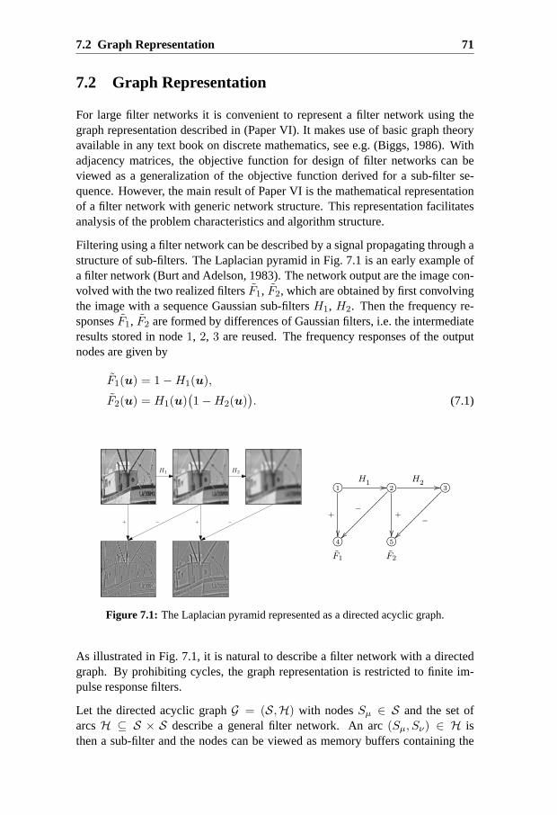
7.2 Graph Representation 71
7.2 Graph Representation
For large filter networks it is convenient to represent a filter network using thegraph representation described in (Paper VI). It makes use of basic graph theoryavailable in any text book on discrete mathematics, see e.g. (Biggs, 1986). Withadjacency matrices, the objective function for design of filter networks can beviewed as a generalization of the objective function derived for a sub-filter se-quence. However, the main result of Paper VI is the mathematical representationof a filter network with generic network structure. This representation facilitatesanalysis of the problem characteristics and algorithm structure.
Filtering using a filter network can be described by a signal propagating through astructure of sub-filters. The Laplacian pyramid in Fig. 7.1 is an early example ofa filter network (Burt and Adelson, 1983). The network output are the image con-volved with the two realized filtersF1, F2, which are obtained by first convolvingthe image with a sequence Gaussian sub-filtersH1, H2. Then the frequency re-sponsesF1, F2 are formed by differences of Gaussian filters, i.e. the intermediateresults stored in node1, 2, 3 are reused. The frequency responses of the outputnodes are given by
F1(u) = 1 −H1(u),
F2(u) = H1(u)(1 −H2(u)
). (7.1)
H1
+ −
H2
+ −
1
+
H1
// 2
H2
//
+
−
3
−
4
F1
5
F2
Figure 7.1: The Laplacian pyramid represented as a directed acyclic graph.
As illustrated in Fig. 7.1, it is natural to describe a filter network with a directedgraph. By prohibiting cycles, the graph representation is restricted to finite im-pulse response filters.
Let the directed acyclic graphG = (S,H) with nodesSµ ∈ S and the set ofarcsH ⊆ S × S describe a general filter network. An arc(Sµ, Sν) ∈ H isthen a sub-filter and the nodes can be viewed as memory buffers containing the
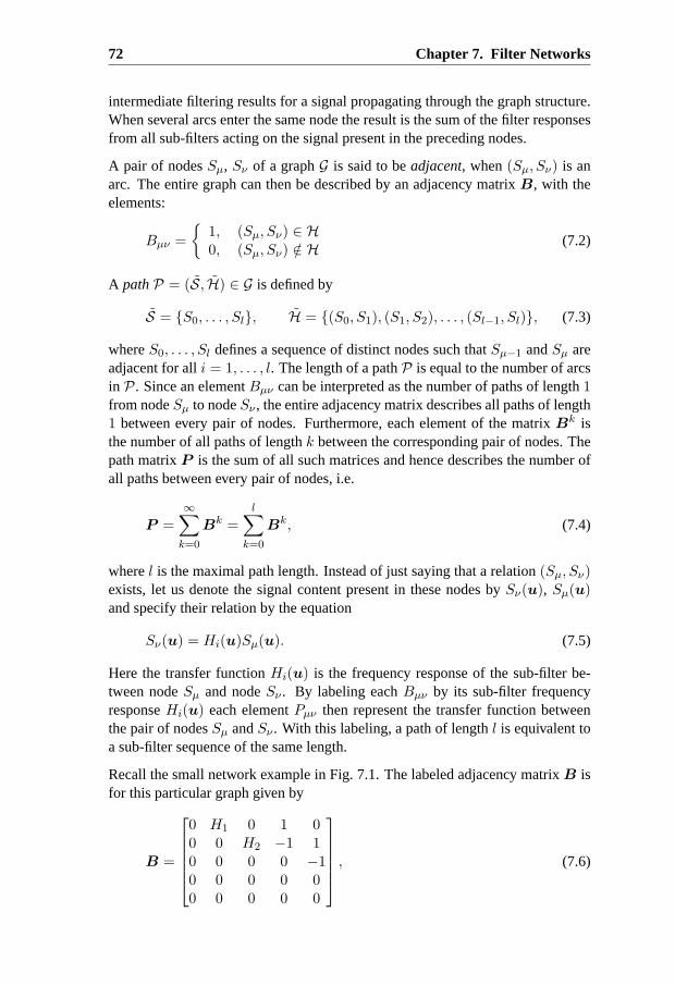
72 Chapter 7. Filter Networks
intermediate filtering results for a signal propagating through the graph structure.When several arcs enter the same node the result is the sum of the filter responsesfrom all sub-filters acting on the signal present in the preceding nodes.
A pair of nodesSµ, Sν of a graphG is said to beadjacent, when(Sµ, Sν) is anarc. The entire graph can then be described by an adjacency matrixB, with theelements:
Bµν =
1, (Sµ, Sν) ∈ H0, (Sµ, Sν) /∈ H (7.2)
A pathP = (S, H) ∈ G is defined by
S = S0, . . . , Sl, H = (S0, S1), (S1, S2), . . . , (Sl−1, Sl), (7.3)
whereS0, . . . , Sl defines a sequence of distinct nodes such thatSµ−1 andSµ areadjacent for alli = 1, . . . , l. The length of a pathP is equal to the number of arcsin P. Since an elementBµν can be interpreted as the number of paths of length1from nodeSµ to nodeSν , the entire adjacency matrix describes all paths of length1 between every pair of nodes. Furthermore, each element of the matrixBk isthe number of all paths of lengthk between the corresponding pair of nodes. Thepath matrixP is the sum of all such matrices and hence describes the number ofall paths between every pair of nodes, i.e.
P =∞∑
k=0
Bk =l∑
k=0
Bk, (7.4)
wherel is the maximal path length. Instead of just saying that a relation(Sµ, Sν)exists, let us denote the signal content present in these nodes bySν(u), Sµ(u)and specify their relation by the equation
Sν(u) = Hi(u)Sµ(u). (7.5)
Here the transfer functionHi(u) is the frequency response of the sub-filter be-tween nodeSµ and nodeSν . By labeling eachBµν by its sub-filter frequencyresponseHi(u) each elementPµν then represent the transfer function betweenthe pair of nodesSµ andSν . With this labeling, a path of lengthl is equivalent toa sub-filter sequence of the same length.
Recall the small network example in Fig. 7.1. The labeled adjacency matrixB isfor this particular graph given by
B =
0 H1 0 1 00 0 H2 −1 10 0 0 0 −10 0 0 0 00 0 0 0 0
, (7.6)
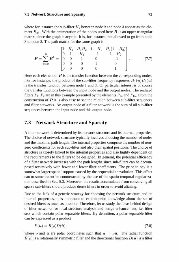
7.3 Network Structure and Sparsity 73
where for instance the sub-filterH2 between node2 and node3 appear as the ele-mentB23. With the enumeration of the nodes used hereB is an upper triangularmatrix, since the graph is acyclic. It is, for instance, not allowed to go from node3 to node2. The path matrix for the same graph is
P =
3∑
k=0
Bk =
1 H1 H1H2 1 −H1 H1(1 −H2)0 1 H2 −1 1 −H2
0 0 1 0 −10 0 0 1 00 0 0 0 1
. (7.7)
Here each element ofP is the transfer function between the corresponding nodes,like for instance, the product of the sub-filter frequency responsesH1(u)H2(u)is the transfer function between node1 and3. Of particular interest is of coursethe transfer functions between the input node and the output nodes. The realizedfilters F1, F2 are in this example presented by the elementsP14 andP15. From theconstruction ofP it is also easy to see the relation between sub-filter sequencesand filter networks. An output node of a filter network is the sum of all sub-filtersequences between the input node and this output node.
7.3 Network Structure and Sparsity
A filter network is determined by its network structure and its internal properties.The choice of network structure typically involves choosing the number of nodesand the maximal path length. The internal properties comprise the number of non-zero coefficients for each sub-filter and also their spatial positions. The choice ofstructure is closely linked to the internal properties and also highly dependent onthe requirements to the filters to be designed. In general, the potential efficiencyof a filter network increases with the path lengths since sub-filters can be decom-posed recursively with fewer and fewer filter coefficients. The price to pay is asomewhat larger spatial support caused by the sequential convolution. This effectcan to some extent be counteracted by the use of the spatio-temporal regulariza-tion described in Sec. 5.3. Moreover, the results accumulated from convolving allsparse sub-filters should produce dense filters in order to avoid aliasing.
Due to the lack of a generic strategy for choosing the network structure and itsinternal properties, it is important to exploit prior knowledge about the set ofdesired filters as much as possible. Therefore, let us study the ideas behind designof filter networks for local structure analysis and image enhancement, i.e. filtersets which contain polar separable filters. By definition, a polar separable filtercan be expressed as a product
F (u) = R(ρ)D(u), (7.8)
whereρ and u are polar coordinates such thatu = ρu. The radial functionR(ρ) is a rotationally symmetric filter and the directional functionD(u) is a filter
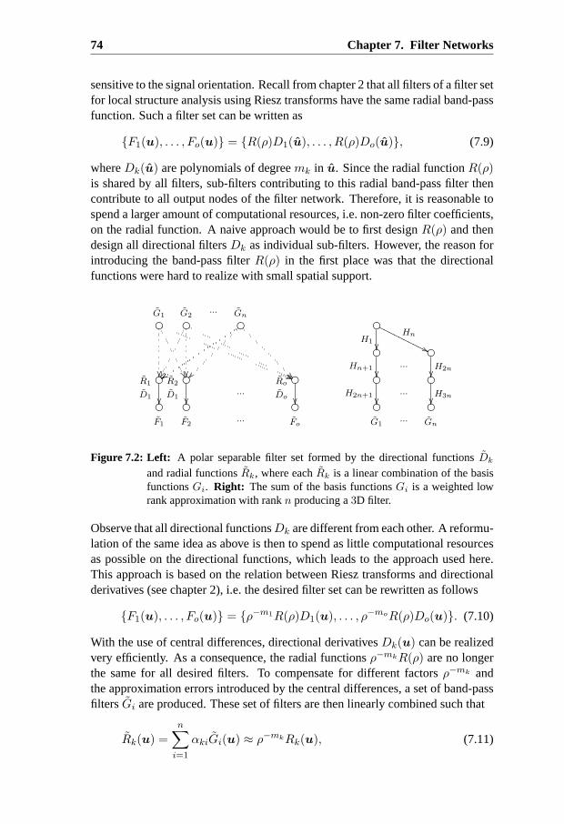
74 Chapter 7. Filter Networks
sensitive to the signal orientation. Recall from chapter 2 that all filters of a filter setfor local structure analysis using Riesz transforms have the same radial band-passfunction. Such a filter set can be written as
F1(u), . . . , Fo(u) = R(ρ)D1(u), . . . , R(ρ)Do(u), (7.9)
whereDk(u) are polynomials of degreemk in u. Since the radial functionR(ρ)is shared by all filters, sub-filters contributing to this radial band-pass filter thencontribute to all output nodes of the filter network. Therefore, it is reasonable tospend a larger amount of computational resources, i.e. non-zero filter coefficients,on the radial function. A naive approach would be to first designR(ρ) and thendesign all directional filtersDk as individual sub-filters. However, the reason forintroducing the band-pass filterR(ρ) in the first place was that the directionalfunctions were hard to realize with small spatial support.
G1
))
G2
''
···
Gn
zz zz
R1
D1
R2
D1
···
Ro
Do
F1
F2 ···
Fo
H1
Hn
''OOOOOOOOOO
Hn+1
···
H2n
H2n+1
···
H3n
G1 ···
Gn
Figure 7.2: Left: A polar separable filter set formed by the directional functionsDk
and radial functionsRk, where eachRk is a linear combination of the basisfunctionsGi. Right: The sum of the basis functionsGi is a weighted lowrank approximation with rankn producing a3D filter.
Observe that all directional functionsDk are different from each other. A reformu-lation of the same idea as above is then to spend as little computational resourcesas possible on the directional functions, which leads to the approach used here.This approach is based on the relation between Riesz transforms and directionalderivatives (see chapter 2), i.e. the desired filter set can be rewritten as follows
F1(u), . . . , Fo(u) = ρ−m1R(ρ)D1(u), . . . , ρ−moR(ρ)Do(u). (7.10)
With the use of central differences, directional derivativesDk(u) can be realizedvery efficiently. As a consequence, the radial functionsρ−mkR(ρ) are no longerthe same for all desired filters. To compensate for different factorsρ−mk andthe approximation errors introduced by the central differences, a set of band-passfilters Gi are produced. These set of filters are then linearly combined such that
Rk(u) =n∑
i=1
αkiGi(u) ≈ ρ−mkRk(u), (7.11)
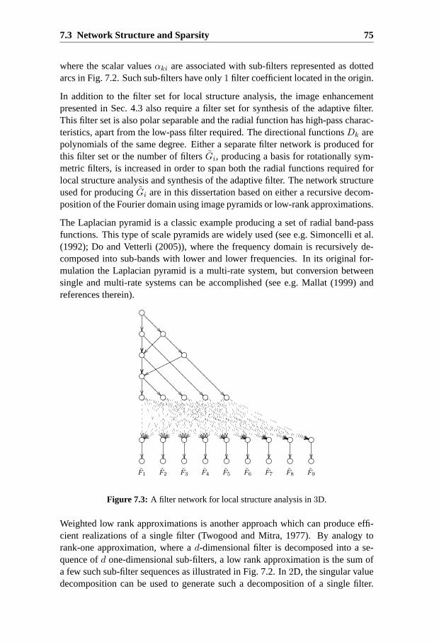
7.3 Network Structure and Sparsity 75
where the scalar valuesαki are associated with sub-filters represented as dottedarcs in Fig. 7.2. Such sub-filters have only1 filter coefficient located in the origin.
In addition to the filter set for local structure analysis, the image enhancementpresented in Sec. 4.3 also require a filter set for synthesis of the adaptive filter.This filter set is also polar separable and the radial function has high-pass charac-teristics, apart from the low-pass filter required. The directional functionsDk arepolynomials of the same degree. Either a separate filter network is produced forthis filter set or the number of filtersGi, producing a basis for rotationally sym-metric filters, is increased in order to span both the radial functions required forlocal structure analysis and synthesis of the adaptive filter. The network structureused for producingGi are in this dissertation based on either a recursive decom-position of the Fourier domain using image pyramids or low-rank approximations.
The Laplacian pyramid is a classic example producing a set of radial band-passfunctions. This type of scale pyramids are widely used (see e.g. Simoncelli et al.(1992); Do and Vetterli (2005)), where the frequency domain is recursively de-composed into sub-bands with lower and lower frequencies. In its original for-mulation the Laplacian pyramid is a multi-rate system, but conversion betweensingle and multi-rate systems can be accomplished (see e.g. Mallat (1999) andreferences therein).
???
???
???
????
????
????
????
?
???
???
???
????
????
??
wwoooooooooo
???
????
????
??
???
???
$$ '' )) ** ** ++
$$ '' )) ** **
$$ '' )) **
zz $$ '' ))
ww zz $$ ''
F1
F2
F3
F4
F5
F6
F7
F8
F9
Figure 7.3: A filter network for local structure analysis in3D.
Weighted low rank approximations is another approach which can produce effi-cient realizations of a single filter (Twogood and Mitra, 1977). By analogy torank-one approximation, where ad-dimensional filter is decomposed into a se-quence ofd one-dimensional sub-filters, a low rank approximation is the sum ofa few such sub-filter sequences as illustrated in Fig. 7.2. In2D, the singular valuedecomposition can be used to generate such a decomposition of a single filter.
76 Chapter 7. Filter Networks
However, to be efficient a few dominant singular values are required, i.e. the de-sired filters must be nearly Cartesian separable. Typically, smooth rotationallysymmetric filters can be realized efficiently with this technique, whereas off-axisanisotropic filters are likely to generate too many singular values.
Putting it all together yields a network structure as the one shown in Fig. 7.3producing a basis which spans the same space as the first and second order Riesztransform in3D. Observe thatGi, Rk andDk are never formed explicitly. Theyare only introduced here in this section to explain the thoughts behind the designchoices made. The only information passed on to the local search method are thespatial constraints imposed on each sub-filter, the network structure, the desiredfrequency responses and an initial point.
7.4 Least Squares Filter Network Design
In the previous chapter, a sub-filter sequence was presented as an approximate fac-torization of a single filter. For a tree-structured network this is still true, but thedifferent realized filters share common factors, since most sub-filters contributeto several output nodes. With a graph structure the desired filter set is decom-posed into a sum of sub-filter sequences, where also filters in parallel branchescan contribute to the same output node.
To find the realizationF1(u), . . . , Fo(u), corresponding to the output nodesof the network, which is as close as possible to the desired frequency responsesF1(u), . . . , Fo(u) this is formulated as a sum of least squares, i.e.
mino∑
k=1
‖εk(u)‖2 =o∑
k=1
∫
U
∣∣Wk(u)
(Fk(u) − Fk(u)
)∣∣2du. (7.12)
Since the choice of the weight functionsW (u) most often reflect the expectedsignal and noise characteristics (see Sec. 5.3), it is natural to chooseW1 = . . . =Wo = W . One exception is when one or a few filters are significantly moredifficult to realize. Then it can be of interest to weight the filters differently inorder to avoid solutions where the errors are concentrated to the filters which aremost difficult to realize. An appropriate choice of scalar valuest1, . . . , to suchthatWk = tkW for k = 1, . . . , o is in that case a remedy to this problem.
Let us denote the input node and the output nodes of the filter network bySinandS1, . . . , So receptively, whereSk corresponds to the realizationFk(u). Sincethe result of several arcs entering a node is the sum of their transfer functions, therealization ofFk can be written compactly as the sum of all pathsp enteringSk:
Fk(u) =∑
p∈Pk
∏
i:Hi∈p
Hi(u) (7.13)

7.5 Implementation 77
Here, each pathp defines a sub-filter sequenceHp1 , . . . , Hpl. The setPk denotes
the set of all paths between the input nodeSin and the output nodeSk defined by
Pk =p ∈ G : p is a path betweenSin andSk
. (7.14)
With the network structure and its internal properties pre-defined problem (7.12)can, in the same way as described in Sec. 5.3, be reduced to the least squaresproblem
mino∑
k=1
‖bk − bk‖2, (7.15)
where the vectorsbk, bk ∈ Rm are obtained by uniform sampling of the frequency
responsesFk(u), Fk(u). As in the previous two chaptersAi, xi are the individ-ual characteristics of each sub-filterHi. The vectorbk is then thel:th degreepolynomial inxi defined by
bk =∑
p∈Pk
(Ap1xp1) . . . (Aplxpl
), (7.16)
whereu v denotes the component-wise product of the vectorsv andv and theindex setp1, . . . , pl points out all the sub-filters involved to form the pathp.
The characteristics of the multi-linear least squares problem (7.15) are similar tothe design problem associated with sub-filter sequences in the previous chapter.Since it suffers from the same multi-extremal nature any local search method willbe sensitive to the choice of initial point. Generalization of the approach used togenerate robust initial points presented in Sec. 6.4 is not straightforward, sincethe frequency responses here can not be written as a product of the frequency re-sponses of every sub-filter. In (Andersson et al., 1999) and (Paper V) the filternetworks were designed using alternating least squares (see Sec. 6.3.1). This ap-proach is however not efficient enough, when trying to realize larger filter sets.This is because each iteration becomes computationally expensive not only interms of the number of computations, but also in terms of memory consumption.These were the main motivations for the development of the local search methoddescribed in the next section.
7.5 Implementation
In non-linear least squares, the Jacobian matrix is the key tool to exploit the spe-cial structure of such problems. It is used for computing the gradient, but moreimportantly it also allows efficient computation of the exact or approximate Hes-sian matrix of the function to be minimized. This fits nicely into the frameworkfor filter network design, since it is fairly easy to derive and compute the Jacobianmatrix.
78 Chapter 7. Filter Networks
Let us denote the objective function
ψ(x1, . . . ,xq) =1
2
o∑
k=1
‖rk(x1, . . . ,xq)‖2, (7.17)
whererk = bk − bk ∈ Rm andq is the total number of sub-filters.
For non-linear least squares the gradient can be expressed in terms of the residualvectorr = [r1, . . . , ro]
T ∈ Rmq and the Jacobian matrixJ :
∇ψ = JTr (7.18)
The partial derivatives ofr with respect tox defines the Jacobian matrix, i.e.
J =
∂r1
∂x1· · · ∂r1
∂xq
.... . .
...∂rk
∂x1· · · ∂rk
∂xq
, (7.19)
whereJTJ is a good model of the Hessian, when either residualsr are small orwhen ther is nearly linear, i.e. when the second order derivatives ofr are small.
Now, let us make use of the graph representation to derive the partial derivativesnecessary to compute the Jacobian matrix. The contribution of a single sub-filterto a specific output node can be studied using the path matrixP introduced inSec. 7.2. Let us consider the expression
P (u) = P0µ(u)Pµν(u)Pνk(u), (7.20)
whereP0µ is the transfer function from the input nodeSin to nodeSµ andPνkis the transfer function from nodeSν to the output nodeSk. The transfer func-tion P (u) is then the contribution to the output nodeSk from all paths that passthrough the sub-filter(Sµ, Sν) as illustrated in Fig. 7.4.
Let us denote this sub-filterHi, with individual characteristicsAi, xi. Uniformsampling of the frequency domain reducesP (u) to
p = pik (Aixi), (7.21)
wherepik ∈ Rm corresponds to the productP0µPνk. The partial derivatives∂rk
∂xi
is then given by:
∂rk
∂xi= − ∂
∂xibk = −diag(pik)Ai (7.22)
As shown experimentally in Sec. 6.5 the introduction of symmetry constraintscan help to reduce the number of design variables and hence also the numberof local minima. Another way to accomplish this is to introduce dependencies

7.6 Experiments 79
???
???
Sµ
ww
Sν
???
???
???
????
????
??
$$ '' )) ** ** ++
//////////
$$ '' )) ** **
$$ '' )) **
zz $$ '' ))
ww zz $$ ''
F1
F2
F3
F4
F5
F6
F7
F8
F9
Figure 7.4: All paths (drawn as solid arcs) from the input node that pass through thesub-filter(Sµ, Sν) and contribute to the filterF3.
between different sub-filters. In contrast to the alternating least squares approachpreviously used, this approach allows such dependencies. Suppose that the filtersx1, . . . ,xn are related to the filterxi by xj = Cjxi for j = 1, . . . , n. Using thesame notation as before, the partial derivatives∂rk
∂xinow becomes
∂rk
∂xi= − ∂
∂xibk = −diag(pik)Ai −
∑
j 6=i
diag(pjk)AjCj (7.23)
This might seem as an insignificant improvement but it can in practice be veryimportant since the number of design variables and local minima is large. For thesame reason it is also important to impose symmetry constraints on the individualsub-filters whenever possible (see Sec. 5.4). Similar to design of sub-filter se-quences, regularization of each individual sub-filter helps to prevent undesirablescaling of the problem.
7.6 Experiments
A number of filter network realizations has been produced for local structure anal-ysis and image enhancement related to the work presented in this dissertation.Since the difference between a conventional filter set and a realization with filternetworks can be made arbitrary small by increasing the number of filter coeffi-cients, the difference in performance is often insignificant. In general, the net-works are designed such that they have essentially the same fit to the desired fre-quency response as a FIR filter set. However, since filter networks typically have
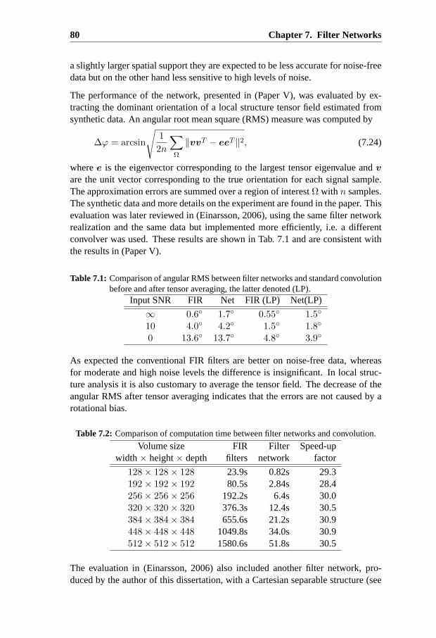
80 Chapter 7. Filter Networks
a slightly larger spatial support they are expected to be less accurate for noise-freedata but on the other hand less sensitive to high levels of noise.
The performance of the network, presented in (Paper V), was evaluated by ex-tracting the dominant orientation of a local structure tensor field estimated fromsynthetic data. An angular root mean square (RMS) measure was computed by
∆ϕ = arcsin
√
1
2n
∑
Ω
‖vvT − eeT ‖2, (7.24)
wheree is the eigenvector corresponding to the largest tensor eigenvalue andv
are the unit vector corresponding to the true orientation for each signal sample.The approximation errors are summed over a region of interestΩ with n samples.The synthetic data and more details on the experiment are found in the paper. Thisevaluation was later reviewed in (Einarsson, 2006), using the same filter networkrealization and the same data but implemented more efficiently, i.e. a differentconvolver was used. These results are shown in Tab. 7.1 and are consistent withthe results in (Paper V).
Table 7.1: Comparison of angular RMS between filter networks and standard convolutionbefore and after tensor averaging, the latter denoted (LP).
Input SNR FIR Net FIR (LP) Net(LP)
∞ 0.6 1.7 0.55 1.5
10 4.0 4.2 1.5 1.8
0 13.6 13.7 4.8 3.9
As expected the conventional FIR filters are better on noise-free data, whereasfor moderate and high noise levels the difference is insignificant. In local struc-ture analysis it is also customary to average the tensor field. The decrease of theangular RMS after tensor averaging indicates that the errors are not caused by arotational bias.
Table 7.2: Comparison of computation time between filter networks and convolution.
Volume size FIR Filter Speed-upwidth× height× depth filters network factor
128 × 128 × 128 23.9s 0.82s 29.3192 × 192 × 192 80.5s 2.84s 28.4256 × 256 × 256 192.2s 6.4s 30.0320 × 320 × 320 376.3s 12.4s 30.5384 × 384 × 384 655.6s 21.2s 30.9448 × 448 × 448 1049.8s 34.0s 30.9512 × 512 × 512 1580.6s 51.8s 30.5
The evaluation in (Einarsson, 2006) also included another filter network, pro-duced by the author of this dissertation, with a Cartesian separable structure (see
7.7 Discussion 81
Fig. 7.2). This network has168 non-zero filter coefficients and was evaluatedwith respect to speed. The tests were carried out in Windows XP on a desktop PCwith a 3.2GHz Pentium 4 processor and1 GB of RAM memory. The results areshown in Tab. 7.2. In terms of number of multiplications the computational gainis 9 · 113
168 ≈ 71, compared to the corresponding FIR filter set with9 filters of size11 × 11 × 11. The now2 year old prototype implementation showed a reductionof the computation time by a factor30 compared to standard convolution.
7.7 Discussion
In this chapter least squares design of filter networks was presented. As opposedto the previous chapter the work here has been mainly focused on efficiency of thefiltering. Target applications typically use large filter sets and have high demandson both performance and computation time. In particular3D filter sets has beenstudied where filter networks can make an important difference. As demonstrated,the use of filter networks produce realizations of3D filter sets which significantlyreduce the computational load of filtering.
The most recent efforts, spent on the local search method, is an important im-provement since optimization of large3D filter sets and4D filters was infeasiblewith the previously used alternating least squares procedure. The efficient searchmethod also facilitates the user interaction necessary to provide an initial guesswhich produce a good filter network. How to optimally choose the network struc-ture and the internal properties remains an open question. The local search methoddoes, however, optimize a typical2D filter set in a few seconds which enables ex-ploration of this search space associated with the internal properties in reasonablecomputation time.


8Review of Papers
The papers included in the second part of this dissertation are here introducedand they appear in the order that best matches the dissertation outline. The paperscover most of the material presented in chapter (2-7). Some chapters provide moredetails than the presentation in the corresponding paper, whereas some chaptersprovide more brief presentations.
8.1 Paper I: On Geometric Transformations of LocalStructure Tensors
Geometric transformation of a local structure tensor fields requires knowledgeabout the covariant or contravariant nature of the tensors and the tensor estimates.In this context local structure and orientation are reviewed. The article demon-strates how a tensor field, estimated from an ultrasound image, is transformedfrom a polar coordinate system to a Cartesian coordinate system. It is also shown,how shape measures by eigenvalue analysis can be extracted without transform-ing the tensor field. This is accomplished by taking into account the metric tensorexpressed in polar coordinates.
8.2 Paper II: Estimation of Non-Cartesian Local Struc-ture Tensor Fields
Estimation of non-Cartesian local structure was presented at the ScandinavianConference on Image Analysis (SCIA) in Aalborg. The paper concerns adaptationof filters for estimation of local structure tensor fields in non-Cartesian coordinatesystems without resampling. Experiments were performed on synthetic data bymeasuring an angular root mean square error of the dominant orientation. In thepresence of noise, the presented approach provides more accurate estimates com-pared to estimation after resampling. The approach also requires less amount ofprocessing.
84 Chapter 8. Review of Papers
8.3 Paper III: Efficient 3-D Adaptive Filtering for Medi-cal Image Enhancement
Adaptive filtering using filter networks was presented at IEEE International Sym-posium on Biomedical Imaging (ISBI) in Arlington. The paper illustrates the useof volumetric processing for medical image enhancement. The paper presents themethod known as adaptive anisotropic filtering which is based on local structureanalysis. The method consists of three steps, estimation of local structure, tensorprocessing and reconstruction. Post-processing was applied to volumetric dataacquired with T1-weighted magnetic resonance imaging, magnetic resonance an-giography and computed tomography. The results from post-mortal volumetriccomputed tomography of the orbit, acquired at different radiation doses, indicatethat the processing used allows for a decrease in radiation dose.
8.4 Paper IV: Approximate Spectral Factorization forDesign of Efficient Sub-Filter Sequences
The article presents an approach for efficiently solving the multi-linear leastsquares problem associated with design of sub-filter sequences. To deal withthe multi-extremal nature of this problem, the presented approach first solvefor an initial point by reformulating the original problem to a conceptuallyclose problem. The solution found constitutes a good initial point for furtherrefinement using a local search method and reduce the risk of finding insufficientlocal solutions. In comparison to alternating least squares started from randomlygenerated initial points, experiments show that the presented approach is morerobust and provides better local solutions. It also reduces the computation time,because in order to get comparable results one must run alternating least squaresa sufficiently large number of times.
8.5 Paper V: Filter Networks for Efficient Estimation ofLocal 3-D Structure
Filter networks used for estimation of local3D structure was presented at theIEEE International Conference on Image processing (ICIP) in Genoa. Comparedto standard convolution, the filter network realization produce a filter set with thecomputational load reduced by a factor50. This paper presents the first graph-structured filter network, which is optimized using a least squares design criterionand produces a3D filter set with sparse sub-filters. The efficiency and precisionof the filter network are compared to standard convolution and FFT-based convo-lution.

8.6 Paper VI: A Graph Representation of Filter Networks 85
8.6 Paper VI: A Graph Representation of Filter Net-works
The graph representation, presented in Joensuu at the Scandinavian Conferenceon Image Analysis (SCIA), constitutes a general framework for filter networkdesign that incorporates many already existing methods for decomposition of FIRfilters. The previous requirement of a layered network structure in (Knutssonet al., 1999) was removed. The representation incorporates the network structurein the objective function and compared to the majority of related formulations thegraph is not restricted to have a tree-structure. The graph representation facilitatesanalysis of the filter network design problem and its characteristics.


9Summary and Outlook
In this dissertation a framework for multidimensional filtering has been presentedand discussed. The applications covered are local structure analysis and imageenhancement. This chapter concludes the first part of this dissertation and presentspossible directions for future work.
9.1 Future Research
• The filter networks presented here produce efficient realizations of3D filtersets with a reduction of the computational load up to a factor70. Futurework on implementation will hopefully narrow the gap between this theo-retic gain and the actual gain in terms of computation time. Future workin this direction also includes searching for the hardware acceleration tech-niques best suited for implementing filter networks.
• It would be desirable to make the filter network design process less depen-dent on the initialization. The sparsity patterns for all sub-filters constitutea huge search space and combined with the network structure it becomeseven larger. To be able to explore this search space in reasonable com-putation time the multi-linear least squares problem must be solved moreefficiently. The global search method generating robust initial points forsub-filter sequences is one step in this direction.
• The multi-linear least squares problem associated with design of sub-filtersequences has similar characteristics to the problem of filter network de-sign. The smaller degree of freedom in its structure makes it a good prob-lem for evaluating methods for network pruning as well as global and localsearch methods intended for filter networks. The sub-filter sequences arein themselves interesting and can be seen as a generalization of low-rankapproximation, i.e. they can produce efficient realizations of filters that arenot Cartesian separable.
88 Chapter 9. Summary and Outlook
• This dissertation is one result of two research projects with the goal to pro-duce high speed filtering of multidimensional signals in high quality med-ical image enhancement applications, where the filter networks for localstructure analysis and adaptive anisotropic filtering is the main contribution.This work will not end by this dissertation and evaluation of the results pro-duced with this technique is a continuous process conducted in cooperationwith clinical experts. Filter networks for3D scale-adaptive enhancementand enhancement of volume sequences (4D) are apparent directions for fu-ture work.
• The approach presented for a geometrically correct description of localstructure in non-Cartesian coordinate systems is not only intended for thelimited number of people working with local structure tensors. Quite recenttechnologies in imaging produce tensor fields which are physical measure-ments such as diffusion tensor MRI and strain tensors in elastography. Pro-cessing of such tensor fields are therefore less developed, in particular fornon-Cartesian coordinate systems. Processing in warped coordinate sys-tems, in general, requires the use of multiple scales to take into account thespatially varying metric. Therefore it is another possible application wherefilter networks can be a useful tool.
• The perspective, where local structure is the metric of a vector represen-tation for local phase and orientation, was presented as a review with noapparent application. These representations allow, for instance, local phasemodels to be used in diffusion and variational formulations such as the Bel-trami framework. Such a signal model is believed to experience differentcharacteristics and can therefore be an interesting alternative to the widelyused piece-wise constant signal models. For this purpose the maximallylocalized quadrature filters can be used to ensure small time steps.
There is still a lot of work to be done on filter network design and its applications.So far only a fraction of the range of target applications has been studied. Re-search on this topic can be carried out at many different levels, virtually anythingin between approaching the challenging optimization problem and implement-ing real-time multidimensional filtering with state-of-the-art hardware accelera-tion techniques.

Bibliography
Abramatic, J. F. and Silverman, L. M. (1979). Non-stationary linear restorationof noisy images. InProceedings IEEE Conf. on Decision and Control, pages92–99, Fort Lauderdale, FL.
Ahn, K.-H., Choi, Y., and Lee, S.-Y. (1998). Pruned feed-forward networks for ef-ficient implementation of multiple fir filters with arbitrary frequency responses.Neural Processing Letters, 8(7):221–227.
Allen, J. B. and Rabiner, L. R. (1977). A unified approach to short-time Fourieranalysis and synthesis. InProc. IEEE, volume 65:11, pages 1558–1564.
Andersson, K., Andersson, M., and Knutsson, H. (2001). A perception basedvelocity estimator and its use for motion compensated prediction. InProceed-ings of the 12th Scandinavian Conference on Image Analysis, pages 493–499,Bergen, Norway. SCIA.
Andersson, M. and Knutsson, H. (2003). Transformation of local spatio-temporalstructure tensor fields. InIEEE International Conference on Acoustics Speechand Signal Processing (ICASSP). (Presented at ICIP 2003 in Barcelona, Spain,Sept 20).
Andersson, M., Wiklund, J., and Knutsson, H. (1999). Filter networks. InProceedings of Signal and Image Processing (SIP’99), Nassau, Bahamas.IASTED.
Barash, D. (2002). A fundamental relationship between bilateral filtering, adap-tive smoothing, and the nonlinear diffusion equation.PAMI, 24(6):844–847.
Biggs, N. L. (1986).Discrete mathematics. Oxford University Press, Inc., NewYork, NY, USA.
Bigun, J. and Granlund, G. H. (1987). Optimal orientation detection of linearsymmetry. InIEEE First International Conference on Computer Vision, pages433–438, London, Great Britain.
Boukerroui, D., Noble, J. A., and Brady, M. (2004). On the choice of band-passquadrature filters.Journal of Mathematical Imaging and Vision, 21(1):53–80.
Bracewell, R. (1986).The Fourier Transform and its Applications. McGraw-Hill,2nd edition.
90 Bibliography
Brox, T., Weickert, J., Burgeth, B., and Mrazek, P. (2006). Nonlinear structuretensors.Elsevier Image and Vision Computing, 24:41–55.
Brun, A. (2004). Local minima in sequential FIR filter optimization. Unpublishedtechnical report, Computer Vision Laboratory, Linkoping University.
Brun, A., Westin, C.-F., Herberthson, M., and Knutsson, H. (2005). Fast manifoldlearning based on riemannian normal coordinates. InProceedings of the 14thScandinavian Conference on Image Analysis (SCIA’05), Joensuu, Finland.
Buades, A., Coll, B., and Morel, J. (2005). A review of image denoising algo-rithms, with a new one.Multiscale Modeling and Simulation, 4(2):490–530.
Burgeth, B., Welk, M., Feddern, C., and Weickert, J. (2004). Morphologicaloperations on matrix-valued images.Computer Vision - ECCV 2004. LectureNotes in Computer Science.
Burt, P. J. and Adelson, E. H. (1983). The Laplacian pyramid as a compact imagecode.IEEE Trans. Comm., 31:532–540.
Canny, J. (1986). A computational approach to edge detection.IEEE Transactionson Pattern Analysis and Machine Intelligence, PAMI-8(6):255–274.
Carlsson, G., Ishkhanov, T., Silva, V., and Zomorodian, A. (2008). On the localbehavior of spaces of natural images.Int. J. Comput. Vision, 76(1):1–12.
Chen, S. S., Donoho, D. L., and Saunders, M. A. (2001). Atomic decompositionby basis persuit.SIAM Review, 43(1).
Comaniciu, D. and Meer, P. (2002). Mean shift: A robust approach toward featurespace analysis.IEEE Transactions on Pattern Analysis and Machine Intelli-gence, 24(5):603–619.
Daugman, J. G. (1980). Two-dimensional analysis of cortical receptive field pro-files. Vision Research, 20:447–456.
Do, M. and Vetterli, M. (Dec. 2005). The contourlet transform: an efficient direc-tional multiresolution image representation.Image Processing, IEEE Transac-tions on, 14(12):2091–2106.
Do, M. and Vetterli, M. (Sept. 2003). Framing pyramids.Signal Processing,IEEE Transactions on [see also Acoustics, Speech, and Signal Processing,IEEE Transactions on], 51(9):2329–2342.
Donoho, D. L. (1995). De-noising via soft tresholding.IEEE Transactions onInformation Theory, 41(3):613–627.
Dudgeon, D. E. and Mersereau, R. M. (1990).Multidimensional Digital SignalProcessing. Prentice Hall Professional Technical Reference.
Bibliography 91
Einarsson, H. (2006). Implementation and performance analysis of filternets.Master thesis, Linkoping University.
Elad, M. (Dec. 2006). Why simple shrinkage is still relevant for redundant repre-sentations?Information Theory, IEEE Transactions on, 52(12):5559–5569.
Eslami, R. and Radha, H. (Nov. 2006). Translation-invariant contourlet transformand its application to image denoising.Image Processing, IEEE Transactionson, 15(11):3362–3374.
Farneback, G. (2002). Polynomial Expansion for Orientation and Motion Es-timation. PhD thesis, Linkoping University, Sweden, SE-581 83 Linkoping,Sweden. Dissertation No 790, ISBN 91-7373-475-6.
Felsberg, M. (2002).Low-Level Image Processing with the Structure Multivector.PhD thesis, Institute of Computer Science and Applied Mathematics, Christian-Albrechts-University of Kiel, Germany.
Felsberg, M. and Jonsson, E. (2005). Energy tensors: Quadratic phase invari-ant image operators. InDAGM 2005, volume 3663 ofLNCS, pages 493–500.Springer.
Felsberg, M. and Kothe, U. (2005). Get: The connection between monogenicscale-space and gaussian derivatives. In Kimmel, R., Sochen, N., and Weickert,J., editors,Scale Space and PDE Mathods in Computer Vision, volume 3459 ofLNCS, pages 192–203. Springer.
Felsberg, M. and Sommer, G. (2001). The monogenic signal.IEEE Transactionson Signal Processing, 49(12):3136–3144.
Forstner, W. and Gulch, E. (1987). A fast operator for detection and precise loca-tion of distinct points corners and centres of circular features. InISPRS Inter-commission Workshop, Interlaken.
Freeman, W. T. and Adelson, E. H. (1991). The design and use of steerable filters.IEEE Transactions on Pattern Analysis and Machine Intelligence, 13(9):891–906.
Gabor, D. (1946). Theory of communication.J. Inst. Elec. Eng., 93(26):429–457.
Gorinevsky, D. and Boyd, S. (2006). Optimization-based design and implementa-tion of multidimensional zero-phase iir filters.IEEE Transactions on Circuitsand Systems I, 53(2):372–383.
Granlund, G. H. (1978). In search of a general picture processing operator.Com-puter Graphics and Image Processing, 8(2):155–178.
Granlund, G. H. and Knutsson, H. (1995).Signal Processing for Computer Vision.Kluwer Academic Publishers. ISBN 0-7923-9530-1.
92 Bibliography
Haglund, L. (1992).Adaptive Multidimensional Filtering. PhD thesis, LinkopingUniversity, Sweden, SE-581 83 Linkoping, Sweden. Dissertation No 284,ISBN 91-7870-988-1.
Haglund, L., Knutsson, H., and Granlund, G. H. (1989). On phase representationof image information. InThe 6th Scandinavian Conference on Image Analysis,pages 1082–1089, Oulu, Finland.
Hamarneh, G. and Hradsky, J. (Oct. 2007). Bilateral filtering of diffusion ten-sor magnetic resonance images.Image Processing, IEEE Transactions on,16(10):2463–2475.
Hansen, P. C., Nagy, J. G., and O’Leary, D. P. (2006).Deblurring Images: Ma-trices, Spectra, and Filtering (Fundamentals of Algorithms 3) (Fundamentalsof Algorithms). Society for Industrial and Applied Mathematics, Philadelphia,PA, USA.
Harris, C. and Stephens, M. (1988). A combined corner and edge detection. InProceedings of The Fourth Alvey Vision Conference, pages 147–151.
Herberthson, M., Brun, A., and Knutsson, H. (2007). P-averages of diffusiontensors. InProceedings of the SSBA Symposium on Image Analysis, Linkoping,Sweden. SSBA.
Huang, J. and Mumford, D. (1999). Statistics of natural images and models. InProceedings of IEEE on Computer Vision and Pattern Recognition (CVPR’99),pages 541–547.
Jones, M. N. (1985).Spherical Harmonics and Tensors for Classical Field The-ory. Research Studies Press.
Kimmel, R., Sochen, N. A., and Malladi, R. (1997). From high energy physics tolow level vision. InScale-Space Theories in Computer Vision, pages 236–247,London, UK. Springer-Verlag.
Kingsbury, N. (2001). Complex wavelets for shift invariant analysis and filter-ing of signals. Journal of Applied and Computational Harmonic Analysis,10(3):234–253.
Knutsson, H. (1982).Filtering and Reconstruction in Image Processing. PhDthesis, Linkoping University, Sweden. Diss. No. 88.
Knutsson, H. (1985). Producing a continuous and distance preserving 5-D vectorrepresentation of 3-D orientation. InIEEE Computer Society Workshop onComputer Architecture for Pattern Analysis and Image Database Management- CAPAIDM, pages 175–182, Miami Beach, Florida. IEEE.
Knutsson, H. (1987). A tensor representation of 3-D structures. In5th IEEE-ASSPand EURASIP Workshop on Multidimensional Signal Processing, Noordwijk-erhout, The Netherlands.

Bibliography 93
Knutsson, H. (1989). Representing local structure using tensors. InThe 6th Scan-dinavian Conference on Image Analysis, pages 244–251, Oulu, Finland. ReportLiTH–ISY–I–1019, Computer Vision Laboratory, Linkoping University, Swe-den, 1989.
Knutsson, H. and Andersson, M. (2005). Implications of invariance and uncer-tainty for local structure analysis filter sets.Signal Processing: Image Commu-nications, 20(6):569–581.
Knutsson, H., Andersson, M., and Wiklund, J. (1999). Advanced filter design. InProceedings of the 11th Scandinavian Conference on Image Analysis, Green-land. SCIA.
Knutsson, H. and Granlund, G. H. (1980). Fourier domain design of line andedge detectors. InProceedings of the 5th International Conference on PatternRecognition, Miami, Florida.
Knutsson, H., Haglund, L., and Barman, H. (1991). A tensor based approach tostructure analysis and enhancement in 2D, 3D and 4D. InWorkshop Program,Seventh Workshop on Multidimentional Signal Processing, Lake Placid, NewYork, USA. IEEE Signal Processing Society.
Knutsson, H., Wilson, R., and Granlund, G. H. (1981). Anisotropic filtering con-trolled by image content. InProceedings of the 2nd Scandinavian Conferenceon Image Analysis, Finland.
Knutsson, H., Wilson, R., and Granlund, G. H. (1983). Anisotropic non-stationaryimage estimation and its applications — Part I: Restoration of noisy images.IEEE Transactions on Communications, 31(3):388–397.
Koenderink, J. J. (1984). The structure of images.Biological Cybernetics,50(5):363–370.
Kothe, U. (2003). Integrated edge and junction detection with the boundary ten-sor. In Alamitos, L., editor,Proc. of the 9th Intl. Conf. on Computer Vision,volume 1, pages 424–431, Nice. IEEE Computer Society.
Langer, M., Svensson, B., Brun, A., Andersson, M., and Knutsson, H. (2005).Design of fast multidimensional filters using genetic algorithms. InProceed-ings of EvoIASP, 7th European Workshop on Evolutionary Computing in ImageAnalysis and Signal Processing, pages 366 – 375, Lausanne, Switzerland.
Larkin, K. G., Bone, D. J., and Oldfield, M. A. (2001). Natural demodulationof two-dimensional fringe patterns. i. general background of the spiral phasequadrature transform.J. Opt. Soc. Am. A, 18(8):1862–1870.
Maclennan, B. (1981). Gabor representations of spatiotemporal visual images.Technical Report CS-91-144, Computer Science Department, University ofTennesse.

94 Bibliography
Mallat, S. (1999).A Wavelet Tour of Signal Processing. Academic Press.
Mallat, S. and Zhang, Z. (1993). Matching pursuits with time-frequency dictio-naries.IEEE Transactions on Signal Processing, 41(12):3397–3415.
McClellan, J. H. and Parks, T. W. (1973). A unified approach to the design of op-timum FIR linear phase digital filters.IEEE Trans. Circuit Theory, CT-20:697–701.
Neuvo, Y., Cheng-Yu, D., and Mitra, S. (1984). Interpolated finite impulse re-sponse filters.IEEE Transactions on Acoustics, Speech, and Signal Processing,32(3):563 – 570.
Nocedal, J. and Wright, S. (1999).Numerical Optimization. Springer-Verlag.
Nordberg, K. and Farneback, G. (2005). Estimation of orientation tensors forsimple signals by means of second-order filters.Signal Processing: ImageCommunication, 20(6):582–594.
Pattichis, S. and Bovik, A. C. (2007). Analyzing image structure by multidi-mensional frequency modulation.IEEE Trans. Pattern Anal. Mach. Intell.,29(5):753–766.
Perona, P. and Malik, J. (1990). Scale space and edge diffusion using anisotropicdiffusion. IEEE Transactions on Pattern Analysis and Machine Intelligence,12(7):629–639.
Portilla, J., Strela, V., Wainwright, M., and Simoncelli, E. (Nov. 2003). Imagedenoising using scale mixtures of gaussians in the wavelet domain.Image Pro-cessing, IEEE Transactions on, 12(11):1338–1351.
Roberts, L. G. (1965).Optical and Electro-Optical Information Processing, chap-ter Machine Perception of three-dimensional Solid, pages 159–197. MIT Press.J. T. Tippell, editor.
Rodrigues-Florido, M. A., Krissian, K., Ruiz-Alzola, J., and Westin, C.-F. (2001).Comparison of two restoration techniques in the context of 3d medical imag-ing. In Niessen, W., editor,Fourth International Conference on Medical ImageComputing and Computer-Assisted Intervention (MICCAI’01), pages 1031–1039, Utrecht, Netherlands. Springer Verlag.
Ruiz-Alzola, J., Westin, C.-F., Warfield, S. K., Alberola, C., Maier, S. E., andKikinis, R. (2002). Nonrigid registration of 3d tensor medical data.MedicalImage Analysis, 6(2):143–161.
Saramaki, T. and Fam, A. (1988). Subfilter approach for designing efficient FIRfilters. InProceedings IEEE International Symposium on Circuits and Systems,pages 2903–2915.
Bibliography 95
Scherzer, O. and Weickert, J. (2000). Relations between regularization and diffu-sion filtering.Journal of Mathematical Imaging and Vision, 12:43–63.
Simoncelli, E. P., Freeman, W. T., Adelson, E. H., and Heeger, D. J.(1992). Shiftable multiscale transforms.IEEE trans. on Information Theory,38(2):587–607.
Sochen, N., Kimmel, R., and Malladi, R. (1998). A general framework for lowlevel vision. IEEE Transactions on Image Processing, 7(3):310–318.
Sonka, M., Hlavac, V., and Boyle, R. (1998).Image Processing, Analysis, andMachine Vision. Thomson-Engineering.
Starck, J., Candes, E., and Donoho, D. (2002). The curvelet transform for imagedenoising.IEEE Transactions on Image Processing, 11(6).
Starck, J.-L., Fadili, J., and Murtagh, F. (Feb. 2007). The undecimated waveletdecomposition and its reconstruction.Image Processing, IEEE Transactionson, 16(2):297–309.
Swindale, N. V. (1996). Looking into a klein bottle.Current Biology, 6(7):776–779.
Takeda, H., Farsiu, S., and Milanfar, P. (2007). Higher order bilateral filters andtheir properties. InProceedings of the SPIE Conf. on Computational Imaging,San Jose.
Tanaka, S. (1995). Topological analysis of point singularities in stimulus prefer-ence maps of the primate visual cortex.Proceedings of the Royal Society ofLondon, Series B, 261:81–88.
Tomasi, C. and Manduchi, R. (1998). Bilateral filtering for gray and color images.In IEEE International Conference on Computer Vision, pages 839–846.
Tufts, D. W. and Francis, J. T. (1970). Designing digital low pass filters - Com-parison of some methods and criteria.IEEE Trans. Audio Electroacoust., AU-18:487–494.
Twogood, R. and Mitra, S. (1977). Computer-aided design of separable two-dimensional digital filters.IEEE Transactions on Acoustics, Speech, and SignalProcessing, 25(2):165 – 169.
Unser, M. (Apr 2000). Sampling-50 years after shannon.Proceedings of theIEEE, 88(4):569–587.
Weickert, J. (1997). A review of nonlinear diffusion filtering. InScale-SpaceTheory in Computer Vision, Lecture Notes in Comp. Science, volume 1252.
Weickert, J. (2001). Applications of nonlinear diffusion in image processing andcomputer vision.Acta Mathematica Universitatis Comenianae, 70(1):33–50.
96 Bibliography
Westin, C.-F. (1991). Feature extraction based on a tensor image description.Thesis No. 288, ISBN 91-7870-815-X.
Westin, C.-F., Richolt, J., Moharir, V., and Kikinis, R. (2000). Affine adaptivefiltering of CT data.Medical Image Analysis, 4(2):161–172.
Westin, C.-F., Wigstrom, L., Loock, T., Sjoqvist, L., Kikinis, R., and Knutsson,H. (2001). Three-dimensional adaptive filtering in magnetic resonance angiog-raphy.Journal of Magnetic Resonance Imaging (JMRI), 14:63–71.
Wiklund, J. and Knutsson, H. (1996). A generalized convolver. Report LiTH-ISY-R-1830, Computer Vision Laboratory, SE-581 83 Linkoping, Sweden.
Wong, W., Chung, A., and Yu, S. (April 2004). Trilateral filtering for biomed-ical images.Biomedical Imaging: Nano to Macro, 2004. IEEE InternationalSymposium on, 1:820–823.
Zhang, T. and Golub, G. (2001). Rank-one approximation to high order tensors.Matrix Analysis and Applications, 23:534–550.
![H2E: A Privacy Provisioning Framework for Collaborative Filtering … · 2019-09-10 · collaborative filtering, content-based filtering, and hybrid filtering [3]. Content-based filtering,](https://img.pdfslide.us/doc/110x75/5f2811153d39b70bb31af3b8/h2e-a-privacy-provisioning-framework-for-collaborative-filtering-2019-09-10-collaborative.jpg)


![10-1 Lesson 10 Objectives Chapter 4 [1,2,3,6]: Multidimensional discrete ordinates Chapter 4 [1,2,3,6]: Multidimensional discrete ordinates Multidimensional](https://img.pdfslide.us/doc/110x75/5697bff81a28abf838cbf777/10-1-lesson-10-objectives-chapter-4-1236-multidimensional-discrete-ordinates.jpg)